A Statistical Model for Stroke Outcome Prediction and Treatment Planning

Abstract

Stroke is a major cause of mortality and long–term disability in the world. Predictive outcome models in stroke are valuable for personalized treatment, rehabilitation planning and in controlled clinical trials. In this paper we design a new model to predict outcome in the short-term, the putative therapeutic window for several treatments. Our regression-based model has a parametric form that is designed to address many challenges common in medical datasets like highly correlated variables and class imbalance. Empirically our model outperforms the best–known previous models in predicting short–term outcomes and in inferring the most effective treatments that improve outcome.

1 Introduction

Stroke is the second–leading cause of death and the leading cause of serious long–term disability in the world; it is the fifth–leading cause of death in the USA with an estimated annual economic burden of $34 billion [15]. About 87% of all strokes are ischemic strokes where blood flow to the brain is blocked [15]. Discovering risk factors, predicting outcome, mortality and complications, planning patient rehabilitation and treatment are all active areas of research within both medical and machine learning communities [12, 14, 19].

Stroke impairs many critical neurological functions, causing a broad range of physical and social disabilities. The final outcome after a stroke can range from complete recovery to permanent disability and death. Accurate outcome prediction has several uses: to guide treatment decisions, set prognostic expectations, plan rehabilitation, and select patients in controlled clinical trials. Many outcome models have been proposed that differ mainly in the risk factors used as predictors, for example, [11, 2, 18] that use clinical and imaging variables to predict outcome at 3–6 months after stroke, and [7, 13, 16] using only a few clinical variables for predicting outcome and mortality at 3–9 months.

The modified Rankin scale, shown in table 1, is a quantified measure of disability and has been widely used to evaluate stroke outcomes [23]. The validity and reliability of the scale has been extensively studied and attested [3].

1	No symptoms at all
2	No significant disability despite symptoms; able to carry out all usual duties and activities
3	Slight disability; unable to carry out all previous activities, but able to look after own affairs without assistance
4	Moderate disability; requiring some help, but able to walk without assistance
5	Moderately severe disability; unable to walk without assistance and unable to attend to own bodily needs without assistance
6	Severe disability; bedridden, incontinent and requiring constant nursing care and attention
7	Dead

Table 1: Modified Rankin Scale [23]

The aim of this work is to design a statistical model that can (1) predict short–term stroke outcome in a patient and (2) infer the treatments that are most influential in affecting outcome. Stroke treatment must be tailored to the individual based on identification of the risk of damage and estimation of potential recovery [9], and is one of the most important uses of outcome models. However existing outcome models use only a small number of predictive factors and are considered to be unreliable for guiding treatments (see [6, 8] for details). In this study, we model the outcome using 6 past conditions, 3 demographic variables, 16 clinical variables, 23 treatment variables and the admission Rankin score (that measures the patient’s initial condition).

Unlike previous outcome models, our model is designed to learn the factors that affect outcome in the short–term, between admission and discharge, that is believed to be the therapeutic window for neuroprotective drugs and thrombolysis [24], although our model can be used to predict long–term effects as well. To our knowledge, no previous work has studied the combined effects of risk factors and treatment options, for short–term outcome prediction.

1.0.1 Modeling Challenges

The modeling problem can be viewed as follows.

A subject with initial condition $c_{I}$ progresses to a final condition $c_{F}$. During this transition the subject’s state and the factors affecting it are represented by features $Y$. The state of the subject before condition $c_{I}$ is represented by features $X$. Conditions $c_{I},c_{F}$ are typically quantified by a discrete, ordinal scale.

Such problems occur commonly, though not exclusively, in healthcare. E.g. in this study, $c_{I}$ is quantified by the patient’s Rankin score at hospital admission, and $c_{F}$ by the Rankin score at discharge, $X$ represents features like past conditions and $Y$ represents treatments or procedures undertaken during the hospital stay. Our aim is to build a predictive model for (the value at) $c_{F}$ using predictors $X,Y,c_{I}$, while addressing the following challenges.

• High Correlation. When the time elapsed between $c_{I}$ and $c_{F}$ is short, e.g. between hospital admission and discharge, and if the effects of $Y$ are not easily discernible, $c_{I}$ and $c_{F}$ are highly correlated. In such cases, using $c_{I}$ as a predictor of $c_{F}$ (like in a simple Logistic Regression model) results in it masking the effect of all the variables in $Y$. This results in trivial predictions (predicted value of $c_{F}$ equals that of input $c_{I}$) and makes it impossible to infer the effects of $Y$ on the final condition.

  Note there are no assumptions on the correlation among the predictors $X,Y,c_{I}$ and techniques like Principal Components Analysis (PCA) may be applied to obtain uncorrelated features. This still does not solve the problem of high correlation with the outcome variable, $c_{F}$.

• Multiple Classes. Each of the states can have multiple levels, e.g. 7 levels for Rankin score. It is possible to build separate classification models for each pair $(c_{I},c_{F})$ or for each initial condition $c_{I}$, but such models are unable to utilize all the information present in the data, as we show empirically.

• Data Imbalance. Due to the high correlation present, most of the subjects begin and end with the same level in $c_{I},c_{F}$. Observations with different conditions, $c_{I}\neq c_{F}$, are far fewer in number leading to the classical problem of imbalance prevalent in many medical datasets [22, 17].

• Small Datasets. Many clinical studies are conducted on small groups of volunteers and such datasets are typically small. The presence of imbalance, multiple classes, correlations and high dimensional features makes the modeling task even more challenging on such datasets.

• Missing Data. Medical datasets often contain missing values mainly because not all measurements/investigations are done for all patients. While many previous works have addressed missing value imputation for continuous data, few have satisfactorily dealt with discrete data.

1.0.2 Our Contributions

1. We present a new regression–based model for predicting the value of $c_{F}$ using $X,Y,c_{I}$. When used for predicting short–term stroke outcome it achieves significantly higher accuracy than the best–known previous models. The parametric form of our model is designed to address the challenges listed that are prevalent in clinical datasets.

2. Our model allows us to infer the most effective treatments in influencing outcome and are independently validated by previous clinical studies. Other competitive models are unable to produce similar clinically justifiable inferences.

3. We present a new technique for imputing missing categorical data, that achieves higher accuracy than state-of-the-art multiple imputation methods.

2 Our New Model

Let $N$ be the total number of observations in the (training) data. Let $X_{N\times L}$ denote the feature matrix relevant prior to condition $c_{I}$, we use $x_{k}$ to denote the $L$–dimensional feature vector for observation $k$. Similarly, we use $Y_{N\times M}$ and $y_{k}$, respectively, to denote the feature matrix and $M$–dimensional feature vector for observation $k$, relevant between $c_{I}$ and $c_{F}$. See table 5 for examples of such features in our stroke dataset. Let conditions $c_{I},c_{F}$ be measured on an integral scale of 1 to $K$. The $K\times K$ contingency table, $\Omega$, below shows the number of subjects (in training), $n_{i,j}$ with condition $c_{I}=i$ and condition $c_{F}=j$, where $i=1,\ldots K;j=1,\ldots K$.

$$\kern 0.0pt\kern 2.5pt\kern-5.0pt\left[\kern 0.0pt\kern-2.5pt\kern-5.55557pt\vbox{\kern-0.86108pt\vbox{\vbox{ \halign{\kern\arraycolsep\hfil\@arstrut$\kbcolstyle#$\hfil\kern\arraycolsep& \kern\arraycolsep\hfil$\@kbrowstyle#$\ifkbalignright\relax\else\hfil\fi\kern\arraycolsep&& \kern\arraycolsep\hfil$\@kbrowstyle#$\ifkbalignright\relax\else\hfil\fi\kern\arraycolsep\cr 5.0pt\hfil\@arstrut$\scriptstyle\mbox{Score}$\hfil\kern 5.0pt&5.0pt\hfil$\scriptstyle 1$\hfil\kern 5.0pt&5.0pt\hfil$\scriptstyle..$\hfil\kern 5.0pt&5.0pt\hfil$\scriptstyle j$\hfil\kern 5.0pt&5.0pt\hfil$\scriptstyle..$\hfil\kern 5.0pt&5.0pt\hfil$\scriptstyle K\\1$\hfil\kern 5.0pt&5.0pt\hfil$\scriptstyle n_{1,1}$\hfil\kern 5.0pt&5.0pt\hfil$\scriptstyle..$\hfil\kern 5.0pt&5.0pt\hfil$\scriptstyle n_{1,j}$\hfil\kern 5.0pt&5.0pt\hfil$\scriptstyle..$\hfil\kern 5.0pt&5.0pt\hfil$\scriptstyle n_{1,K}\\:$\hfil\kern 5.0pt&5.0pt\hfil$\scriptstyle..$\hfil\kern 5.0pt&5.0pt\hfil$\scriptstyle..$\hfil\kern 5.0pt&5.0pt\hfil$\scriptstyle..$\hfil\kern 5.0pt&5.0pt\hfil$\scriptstyle..$\hfil\kern 5.0pt&5.0pt\hfil$\scriptstyle..\\i$\hfil\kern 5.0pt&5.0pt\hfil$\scriptstyle n_{i,1}$\hfil\kern 5.0pt&5.0pt\hfil$\scriptstyle..$\hfil\kern 5.0pt&5.0pt\hfil$\scriptstyle n_{i,j}$\hfil\kern 5.0pt&5.0pt\hfil$\scriptstyle..$\hfil\kern 5.0pt&5.0pt\hfil$\scriptstyle n_{i,K}\\:$\hfil\kern 5.0pt&5.0pt\hfil$\scriptstyle..$\hfil\kern 5.0pt&5.0pt\hfil$\scriptstyle..$\hfil\kern 5.0pt&5.0pt\hfil$\scriptstyle..$\hfil\kern 5.0pt&5.0pt\hfil$\scriptstyle..$\hfil\kern 5.0pt&5.0pt\hfil$\scriptstyle..\\K$\hfil\kern 5.0pt&5.0pt\hfil$\scriptstyle n_{K,1}$\hfil\kern 5.0pt&5.0pt\hfil$\scriptstyle..$\hfil\kern 5.0pt&5.0pt\hfil$\scriptstyle n_{K,j}$\hfil\kern 5.0pt&5.0pt\hfil$\scriptstyle..$\hfil\kern 5.0pt&5.0pt\hfil$\scriptstyle n_{K,K}\\$\hfil\kern 5.0pt\crcr}}}}\right]$$

Given the data, the likelihood can be modelled as a multinomial probability subject to the condition $\sum\limits_{j=1}^{K}p(i\rightarrow j|x_{k},y_{k})=1,\forall i,k.$ (ignoring parameter–-independent normalization constants):

$$L(\theta)\propto\prod\limits_{k=1}^{N}\prod\limits_{i=1}^{K}\prod\limits_{j=1}^{K-1}\{{p(i\rightarrow j|x_{k},y_{k})}^{r_{k,i}c_{k,j}}\}\{1-\sum\limits_{j=1}^{K-1}{p(i\rightarrow j|x_{k},y_{k})}\}^{r_{k,i}c_{k,K}}$$

$r_{k,i}=\begin{cases}1,&\text{if the $k^{th}$ observation has $c_{I}=i$ ($i^{th}$ row) }\\ 0,&\text{otherwise}\end{cases}$

$c_{k,j}=\begin{cases}1,&\text{if the $k^{th}$ observation has $c_{F}=j$ ($j^{th}$ column)}\\ 0,&\text{otherwise}\end{cases}$

where $p(i\rightarrow j|x_{k},y_{k})$ is the probability of a subject with condition $c_{F}=j$, given features $x_{k},y_{k}$ and initial condition $c_{I}=i$. We propose the following form for $p(i\rightarrow j|x_{k},y_{k})$:

$$p(i\rightarrow j|x_{k},y_{k})=\frac{\lambda_{i}(x_{k})}{\alpha+\lambda_{i}(x_{k})+K_{ij}\,\gamma_{j}(y_{k})}$$

where:

$\lambda_{i}({x_{k}})=\text{exp}(\beta_{0i}+\sum\limits_{l=1}^{L}\beta_{li}\,x_{kl})$, denotes the effects of features $x_{k}$ on the initial condition $c_{I}$ ($i^{th}$ row effect). $\gamma_{j}({y_{k}})=\text{exp}(\delta_{0j}+\sum\limits_{m=1}^{M}\delta_{mj}\,y_{km})$, denotes the effects of features $y_{k}$ on the final condition $c_{F}$ ($j^{th}$ column effect). $K_{ij}=C\*\{(j-i)^{2}+1\}$; C and $\alpha$ are constants.

We now justify our choice of this parametric form.

1. The row effects $\lambda_{i}(x_{k})$ depend only on features relevant before $c_{I}$ while the column effects $\gamma_{j}(y_{k})$ depend on features relevant between $c_{I}$ and $c_{F}$.

2. One of our objectives is to also find which features $y_{k}$ lead to an improvement in the subject’s condition, i.e. $c_{F}<c_{I}$. Since $y_{k}$ appears only in the denominator, feature coefficients with the least values (most negative) will have the maximum impact in improvement.

3. Since the model is purely probabilistic, distributions of these coefficients can be derived and hence p–values can be computed, to test the significance of the features.

4. In small datasets with imbalance, the contingency matrix has higher numbers along the diagonals (i.e., most subjects with $c_{I}=i$ remain at $c_{F}=i$), with the number of subjects decreasing gradually as we move away from the diagonal (e.g. a transition from 3, to 2 or 4 is more likely than to 1 or 5). Observing this pattern, we deliberately introduce the term $K_{i,j}$, which increases the probability value if i is close to j. The constant $C$ plays the role of weights used in cost–sensitive learning algorithms for imbalanced data classification [25]. In our case the imbalance is between diagonal and off–diagonal elements in the contingency table. A higher value of $C$ increases the weight of off–diagonal elements which helps when there are very few off–diagonal elements. Strategies similar to those used in imbalanced data learning can be adopted to choose C, e.g. C can be chosen to be $\frac{n_{d}}{n_{o}}$ where $n_{d}=\Sigma n_{i,i}$ is the number of diagonal elements and $n_{o}=N-n_{d}$, is the number of off–diagonal elements.

5. The constant $\alpha=0.001$ is added to the denominator to handle model identifiablity problems. Without the term, multiplying the numerator and denominator by a constant does not affect the probability but changes the coefficient estimates, necessitating constraints on the parameters. Thus, we add a small constant that ensures unique estimates without affecting the likelihood.

2.0.1 Advantages of our Approach

• By not taking $c_{I}$ as a feature directly, we overcome the problem of $c_{I}$ being highly correlated to $c_{F}$. If $c_{I}$ were to be taken as a feature in a classifier (like Logistic Regression), it is given the the highest significance and the rest of the features are ignored (with zero or nearly zero coefficients). Such a classifier fails to predict well for those subjects whose difference in condition ($c_{F}-c_{I}$) is non–zero. Moreover, it fails to infer the effects of $y_{k}$ on $c_{F}$.

• Simple predictors that predict differences in outcome ($c_{F}-c_{I}$) using features $X,Y$ do not take into account the differences between varying initial and final conditions. For example, a subject with initial condition $c_{I}=3$ and final condition $c_{F}=1$, is different from a subject with $c_{I}=4,c_{F}=2$ and this can affect the predictive performance as seen in our experiments.

• Multiple classifiers can be trained, one for each $c_{I}$ (row). We find that this approach is severely affected by class imbalance and gives trivial predictions $c_{F}=c_{I}$ in almost all cases. In contrast, our approach, for a particular row, takes into account all the observations in the corresponding columns to make the prediction, thus tackling the imbalance and giving better accuracy, as shown empirically. This is particularly helpful while learning from small datasets.

• To compute the probability, say $p(c_{I}=2\rightarrow c_{F}=1)$, we learn from all the subjects with $c_{F}=1$ and from all the subjects with $c_{I}=2$, as opposed to learning from only those subjects with $c_{F}=2$ and $c_{I}=1$ (which a row-wise classifier will do). Intuitively, all subjects with $c_{F}=1$ have some distinguishing characteristics (irrespective of their $c_{I}$ values) and similarly for all subjects with $c_{I}=2$, and our model attempts to capture this information.

2.0.2 Estimation

Maximum likelihood (ML) estimates of parameters are found using gradient ascent. We use elastic net regularization(Ref) with regularization constants $\lambda_{11},\lambda_{12},\lambda_{21}$ and $\lambda_{22}$ ($\lambda_{11}$ and $\lambda_{12}$ are constraints for $\beta$ ’s while $\lambda_{21}$ and $\lambda_{22}$ are constraints for $\delta$ ’s). The log likelihood of the data including the regularization terms is:

$$l(\theta)=\sum\limits_{k=1}^{N}\sum\limits_{i=1}^{K}\sum\limits_{j=1}^{K-1}r_{k,i}c_{k,j}\Bigg{[}\beta_{0i}+\sum\limits_{l=1}^{L}\beta_{li}\,x_{kl}-\mathrm{log}\{\mathrm{exp}(\beta_{0i}+\sum\limits_{l=1}^{L}\beta_{li}\,x_{kl})$$

$$+K_{ij}\,\mathrm{exp}(\delta_{0j}+\sum\limits_{m=1}^{M}\delta_{mj}\,y_{km})+\alpha\}\Bigg{]}\ +\sum\limits_{k=1}^{N}\sum\limits_{i=1}^{K}r_{k,i}c_{k,K}$$

$$log\{1-\sum\limits_{j=1}^{K-1}\frac{\text{exp}(\beta_{0i}+\sum\limits_{l=1}^{L}\beta_{li}\,x_{kl})}{\alpha+\text{exp}(\beta_{0i}+\sum\limits_{l=1}^{L}\beta_{li}\,x_{kl})+K_{ij}\,\text{exp}(\delta_{0j}+\sum\limits_{m=1}^{M}\delta_{mj}\,y_{km})}\}$$

$$+\lambda_{11}\sum\limits_{i=1}^{K}\sum\limits_{l=1}^{L}|{\beta_{li}}|+\lambda_{12}\sum\limits_{i=1}^{K}\sum\limits_{l=1}^{L}{\beta_{li}}^{2}+\lambda_{21}\sum\limits_{j=1}^{K-1}\sum\limits_{m=1}^{M}|{\delta_{mj}}|+$$

$$\lambda_{22}\sum\limits_{j=1}^{K-1}\sum\limits_{m=1}^{M}{\delta_{mj}}^{2}$$

ML estimates have to be obtained for the following $K(L+M+2)-(M+1)$ parameters $\theta=\{\beta_{0i},\beta_{li},\delta_{0j},\delta_{mj}\},i=1,\ldots,K;j=1,\ldots,K-1;l=1,\ldots,L;m=1,\ldots,M$ (since the probabilities sum to 1 in each row, $j$ iterates over only $K-1$ entries). We equate the partial derivatives to zero but these partial derivatives do not have a closed form solution, so we use gradient ascent to solve for the parameters iteratively. The regularization constants are chosen empirically. The complete derivation is shown in the appendix.

2.0.3 Computational Complexity

For a $K\times K$ contingency table, $N$ observations and feature matrices $X_{N\times L}$ and $Y_{N\times M}$, the complexity of estimating all the parameters of our model is $\mathcal{O}(tK^{2}N(L+M))$ where $t$ is the number of iterations of the gradient ascent.

2.0.4 Outcome Prediction and Feature Importance

To predict the final condition $c_{F}$ of a subject given $c_{I},x_{k},y_{k}$, we compute $\hat{p}(i\rightarrow j|x_{k},y_{k})$ from our model (using ML estimates of coefficients), for all $K$ values of j. The predicted final condition is the value $j$ with the maximum probability.

To evaluate the features that lead to improvement in a subject’s condition, instead of using the final condition $c_{F}$, we use an outcome variable $\Delta$, set as follows: $\Delta=1$ if $c_{F}-c_{I}>0$, $\Delta=-1$ if $c_{F}-c_{I}<0$ and $\Delta=0$ if $c_{F}=c_{I}$. The contingency table and model coefficients are recomputed as before. The interpretation of ${p}(i\rightarrow\Delta|x_{k},y_{k})$ now changes to the probability of a subject’s condition to change by $\Delta$ (negative indicating improvement, positive indicating deterioration for the Rankin scale) given the initial condition i and features $X,Y$. To find which features lead to an improvement in outcome, i.e. $\Delta=-1$, we select the features with the smallest $\delta_{m\Delta}$ (coefficients of $y_{km}$) values, with $\Delta=-1$. Influence of feature interactions in the model can be studied by adding additional variables (e.g. $y_{1k}*y_{2k}$) in the y_k vector.

2.0.5 P value Computation

In order to test the significance of a parameter $\delta_{mj},\,\,(m=1,\ldots,M;j=1,\ldots,K)$ pertaining to the features $Y$, we need to test the null hypothesis $H_{0}:\delta_{mj}=0$ against the alternative hypothesis $H_{1}:\delta_{mj}\neq 0$. Let $\widehat{\delta_{mj}}$ denote the observed value and let $T=\widehat{\boldsymbol{\delta_{mj}}}$, the ML estimator, denote our test statistic. The p-value for the two–sided test is $2\times\text{min}\{P_{H_{0}}(T>\widehat{\delta_{mj}}),P_{H_{0}}(T<\widehat{\delta_{mj}})\}$.

Since the null distribution is not known and we do not have a closed form expression for $T$, we use bootstrapping to compute an empirical p–value. We simulate multiple contingency tables $\Omega_{b},\,b=1,\ldots,500$, and estimate the distribution of $T$ from $\Omega_{b}$, under the null hypothesis $\delta_{mj}=0$, without changing the features $X,Y$. Each table $\Omega_{b}$ is initialized to all zeros and then selected table entries $(i,j)$ ($i^{th}$ row, $j^{th}$ column) are incremented by 1 in the following way. For each observation with initial condition $c_{I}=i$, we generate one sample from a multinomial distribution, with probability $\hat{p}(i\rightarrow j|x_{k},y_{k},\delta_{mj}=0))$, and obtain a value of $c_{F}=j$, which gives the selection $(i,j)$. In total $N$ incrementations are done, once for each observation in our real dataset. We thus obtain a bootstrap contingency table $\Omega_{b}$ and different final conditions $c_{F}$ on which we train our model (retaining all other inputs as given) to obtain $\widehat{\delta_{mj}^{b}}$, for the $b^{th}$ bootstrap, which is a sample from $T$ under the null hypothesis. The empirical p-value is $2\times min\{(\sum\limits_{b=1}^{500}{\bf I}_{T>\widehat{\delta_{mj}^{b}}})/500,(\sum\limits_{b=1}^{500}{\bf I}_{T<\widehat{\delta_{mj}^{b}}})/500\}$; ${\bf I}_{c}=1$ if the condition $c$ is true, otherwise 0.

2.1 Imputation using Association Score

Let $(x_{i},z_{i})$ be the $i^{th}$ observation with $z_{i}$ denoting the response variable (the variable to be imputed for feature $Z$), and $x_{i}$, the $p$–dimensional vector of predictors. As in MICE, we impute $z_{i}$ by sampling from one of the values in $Z_{-i}=\{z_{1},\ldots,z_{i-1},z_{i+1},\ldots,z_{N}\}$, the subset of the feature values with no missing values, where $N$ is the total number of observations. For the $k^{th}$ observation with $z_{k}$ not missing, we define a measure of association $\textbf{Q}_{ik}=\frac{\textbf{C}_{ik}-\textbf{D}_{ik}}{\textbf{C}_{ik}+\textbf{D}_{ik}}$ where, $\textbf{C}_{ik}=\sum\limits_{i=1}^{p}{\bf I}_{x_{k,j}=x_{i,j}}$, $\textbf{D}_{ik}=\sum\limits_{i=1}^{p}{\bf I}_{x_{k,j}\neq x_{i,j}}$; $x_{i,j}$ denotes the $i^{th}$ observation for the $j^{th}$ feature, the sum being over all j for which $x_{k,j}$ and $x_{i,j}$ are not missing and ${\bf I}_{c}$ is an indicator function yielding 1 if the condition $c$ is true, otherwise 0. Thus, $C_{ik}$ and $D_{ik}$ respectively denote the number of concordant and discordant pairs between the $i^{th}$ and the $k^{th}$ observations. $Q_{ik}$ is similar to the Kendall’s $\tau$ measure of association, with a higher value of $Q_{ik}$ indicating stronger association. Let $Z=\{z_{q}\}$ be the list of values with $m$ highest association scores $Q_{iq}$. To impute the missing value $z_{i}$, we select a value at random from the list of $Z$. Imputing a single value takes $\mathcal{O}(Np)$ time.

3 Stroke Data Analysis

We retrospectively analyze the data of 275 ischemic stroke patients in the age group of 45 – 75, admitted to St. John’s Hospital The data includes the variables listed in table 5 for each patient. Summary statistics for each of the variables are shown in the appendix. Numerical attributes like investigations are measured in standard units. Other attributes are suitably encoded as binary or categorical data. For example, addictions, preconditions and treatments are binary variables indicating presence or absence. Radiology investigations are encoded into categories indicating normal or abnormal results. Complete details on the encoding are shown in the appendix. Not all investigations are conducted for all the patients and the treatment variables differ across patients resulting in a large number of missing values.

For our dataset, the contingency table, $\Omega$ is as follows:

$$\kern 0.0pt\kern 2.5pt\kern-5.0pt\left[\kern 0.0pt\kern-2.5pt\kern-5.55557pt\vbox{\kern-0.86108pt\vbox{\vbox{ \halign{\kern\arraycolsep\hfil\@arstrut$\kbcolstyle#$\hfil\kern\arraycolsep& \kern\arraycolsep\hfil$\@kbrowstyle#$\ifkbalignright\relax\else\hfil\fi\kern\arraycolsep&& \kern\arraycolsep\hfil$\@kbrowstyle#$\ifkbalignright\relax\else\hfil\fi\kern\arraycolsep\cr 5.0pt\hfil\@arstrut$\scriptstyle\mbox{Score}$\hfil\kern 5.0pt&5.0pt\hfil$\scriptstyle 1$\hfil\kern 5.0pt&5.0pt\hfil$\scriptstyle 2$\hfil\kern 5.0pt&5.0pt\hfil$\scriptstyle 3$\hfil\kern 5.0pt&5.0pt\hfil$\scriptstyle 4$\hfil\kern 5.0pt&5.0pt\hfil$\scriptstyle 5\\1$\hfil\kern 5.0pt&5.0pt\hfil$\scriptstyle 22$\hfil\kern 5.0pt&5.0pt\hfil$\scriptstyle 0$\hfil\kern 5.0pt&5.0pt\hfil$\scriptstyle 0$\hfil\kern 5.0pt&5.0pt\hfil$\scriptstyle 0$\hfil\kern 5.0pt&5.0pt\hfil$\scriptstyle 0\\2$\hfil\kern 5.0pt&5.0pt\hfil$\scriptstyle 40$\hfil\kern 5.0pt&5.0pt\hfil$\scriptstyle 29$\hfil\kern 5.0pt&5.0pt\hfil$\scriptstyle 1$\hfil\kern 5.0pt&5.0pt\hfil$\scriptstyle 0$\hfil\kern 5.0pt&5.0pt\hfil$\scriptstyle 0\\3$\hfil\kern 5.0pt&5.0pt\hfil$\scriptstyle 1$\hfil\kern 5.0pt&5.0pt\hfil$\scriptstyle 44$\hfil\kern 5.0pt&5.0pt\hfil$\scriptstyle 25$\hfil\kern 5.0pt&5.0pt\hfil$\scriptstyle 0$\hfil\kern 5.0pt&5.0pt\hfil$\scriptstyle 2\\4$\hfil\kern 5.0pt&5.0pt\hfil$\scriptstyle 0$\hfil\kern 5.0pt&5.0pt\hfil$\scriptstyle 0$\hfil\kern 5.0pt&5.0pt\hfil$\scriptstyle 38$\hfil\kern 5.0pt&5.0pt\hfil$\scriptstyle 34$\hfil\kern 5.0pt&5.0pt\hfil$\scriptstyle 2\\5$\hfil\kern 5.0pt&5.0pt\hfil$\scriptstyle 0$\hfil\kern 5.0pt&5.0pt\hfil$\scriptstyle 0$\hfil\kern 5.0pt&5.0pt\hfil$\scriptstyle 2$\hfil\kern 5.0pt&5.0pt\hfil$\scriptstyle 15$\hfil\kern 5.0pt&5.0pt\hfil$\scriptstyle 20$\hfil\kern 5.0pt\crcr}}}}\right]$$

$X_{N\times L}$	Demographic: Age, Gender, Religion
	Time: time between stroke event and treatment start
	Addictions: Smoking, Alcohol
	Preconditions: Hypertension, Diabetes, Ischemic Heart Condition, Preceding Fever
$c_{I}$	Initial condition: Rankin Score at admission
$Y_{N\times M}$	Investigations: Hemoglobin, Total Counts, Differential Counts, Platelet, Creatinine, Serum Sodium, Cholesterol, High Density Lipoprotein (HDL), Low Density Lipoprotein (LDL), Triglycerides, Admission Blood Pressure, Electrocardiogram (ECG), Echo, Doppler
	Treatment: Aspirin, Clopidogrel, Atorvastatin, Finofibrate, Edaravon, Citicoline, Heparin, Dalteparin, Enoxaparine, Warfarin, Acitrom, t-PA, , Dabigatran, Anti-hypertensives (ACEI, Beta Channel Blockers, Diuretics, ARB), Other drugs (Piracetam, Mannitol, B-Complex, Pantoprazole, Antibiotics), Physiotherapy
	Others: Type of ward, number of days in hospital, Complication
$c_{F}$	Final Condition: Rankin Score at discharge

Table 2: Stroke Dataset Variables.

3.0.1 Data Preprocessing

Features with values in less than 25% of patients are omitted. We use MICE [5] to impute all continuous valued features and our association based method for imputing categorical features.

We group the Rankin scores into 3 groups: $g_{1}=\{1\}$, $g_{2}=\{2,3\}$ and $g_{3}=\{4,5,6,7\}$ and use these as $K=3$ levels. The reduced contingency table is:

$$\kern 0.0pt\kern 2.5pt\kern-5.0pt\left[\kern 0.0pt\kern-2.5pt\kern-5.55557pt\vbox{\kern-0.86108pt\vbox{\vbox{ \halign{\kern\arraycolsep\hfil\@arstrut$\kbcolstyle#$\hfil\kern\arraycolsep& \kern\arraycolsep\hfil$\@kbrowstyle#$\ifkbalignright\relax\else\hfil\fi\kern\arraycolsep&& \kern\arraycolsep\hfil$\@kbrowstyle#$\ifkbalignright\relax\else\hfil\fi\kern\arraycolsep\cr 5.0pt\hfil\@arstrut$\scriptstyle\mbox{Score}$\hfil\kern 5.0pt&5.0pt\hfil$\scriptstyle g_{1}$\hfil\kern 5.0pt&5.0pt\hfil$\scriptstyle g_{2}$\hfil\kern 5.0pt&5.0pt\hfil$\scriptstyle g_{3}\\g_{1}$\hfil\kern 5.0pt&5.0pt\hfil$\scriptstyle 22$\hfil\kern 5.0pt&5.0pt\hfil$\scriptstyle 0$\hfil\kern 5.0pt&5.0pt\hfil$\scriptstyle 0\\g_{2}$\hfil\kern 5.0pt&5.0pt\hfil$\scriptstyle 41$\hfil\kern 5.0pt&5.0pt\hfil$\scriptstyle 99$\hfil\kern 5.0pt&5.0pt\hfil$\scriptstyle 2\\g_{3}$\hfil\kern 5.0pt&5.0pt\hfil$\scriptstyle 0$\hfil\kern 5.0pt&5.0pt\hfil$\scriptstyle 40$\hfil\kern 5.0pt&5.0pt\hfil$\scriptstyle 71$\hfil\kern 5.0pt\crcr}}}}\right]$$

3.0.2 Simulated Data

We generate additional synthetic data to evaluate the classifiers on datasets by varying the total observations $N$ and number of classes (levels in $c_{I},c_{F}$), $K$. Datasets with different $N$ are obtained by multiplying the reduced contingency table above by 2, 10, 15 and 20. Datasets with different $K$ are obtained from the dataset with $N=5500$ by splitting the rows while maintaining the pattern found in the real data – high diagonal values and off–diagonal values decreasing with increasing distance from the diagonal. Features $X$ and $Y$ are generated by sampling from 6–dimensional normal distributions $\mathcal{N}(\mu^{X},I)$ and $\mathcal{N}(\mu^{Y},I)$ where $\mu^{X}_{i}=(i-1+c_{I})$ and $\mu^{Y}_{i}=(i+3-c_{F}),i=1,\ldots,6$; $I$ denotes the identity matrix.

4 Experimental Results

4.1 Accuracy of Imputation Method

To test the performance of our imputation method, we select only those 211 observations having no missing values in the (binary) treatment features and remove 10% of the values randomly (using these as missing values) from each feature in $X,Y$, and apply both MICE and our imputation method. We check the accuracy of the imputed values which is the proportion of the observations for which the values are correctly imputed. We repeat the experiment 5 times, each time with a different random selection of values to be imputed. Table 3 shows the accuracy obtained by MICE, K-Nearest Neighbor (KNN) imputation [21] and our method which significantly outperforms both the methods.

Method	Mean	SD
KNN	54.5%	5.16
MICE	59.4%	4.02
Our Method	68.7%	3.86

Table 3: Mean imputation accuracy and standard deviation (SD) over 5 runs of our experiment.

We measure the predictive accuracy of our model and compare it with baseline models that have been used in previous stroke outcome studies.

4.1.1 Evaluation Metrics

Accuracy is defined as the proportion of test observations correctly classified. Overestimate error is defined as the proportion of the misclassified test samples, out of the total number of samples, for which the predicted outcome, $\hat{j}$ is greater than the true outcome, $j$; i.e. $\hat{j}>j$. Similarly the underestimate error measures the proportion of underestimates, $\hat{j}<j$. All results shown are over five–fold cross validation.

4.1.2 Baselines

As baselines we use classification methods Logistic Regression and Support Vector Machines in two different ways. First we concatenate $X,Y$, use them as features to predict $(c_{F}-c_{I})$; we denote these classifiers by $LR$ and $SVM$ respectively. Next we train 5 classifiers, one for each value of $c_{I}$ (each row in the contingency table) and use concatenated features $X,Y$ to predict $c_{F}$. Given a test case, based on the admission score ($c_{I}$), we predict using the corresponding classifier. We denote these classifiers by $LR_{row}$ and $SVM_{row}$ respectively. Our method is denoted by NEW.

4.1.3 Simulated Data

The performance of all the classifiers on the simulations are shown in figure 1. We see that the accuracy of NEW is significantly better than all other baselines and, as expected, the performance improves with more data (increasing $N$). We also see that the performance of all classifiers deteriorate as $K$, the number of levels $c_{F},c_{I}$, increase, making multi–class classification harder. However, our method maintains its superiority over baselines in all four cases.

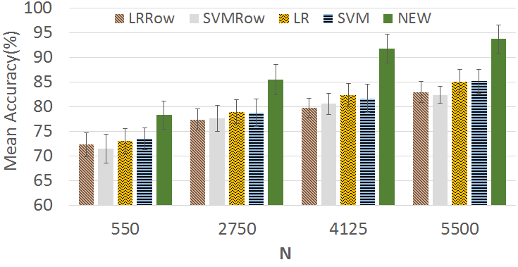
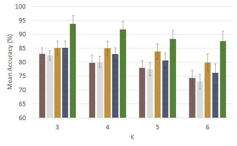
Figure 1: Performance on simulated data with fixed K = 3 and increasing N (above) and fixed N = 5500 and increasing K (below).

4.1.4 Stroke Data

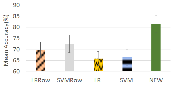
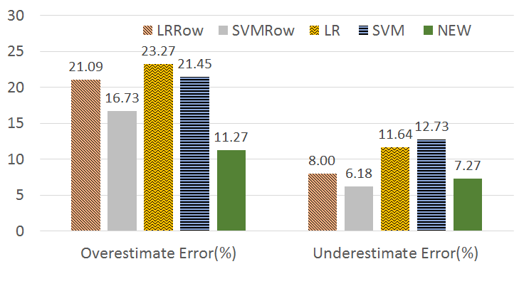
Figure 2: Performance on stroke datset: Mean accuracy over 5–fold cross validation (above); Overestimate and underestimate errors (below).

Figure 2 (above) shows the average predictive accuracy of all the classifiers tested. Logistic Regression (LR) is the best previously used model for predicting outcome and our model outperforms LR by nearly 19%.

Figure 2 (below) shows the overestimate and underestimate errors of all the classifiers. Predicting $\hat{j}>j$ results in overestimating the predicted outcome and may result in overburdening the patients with unnecessary treatments or higher dosages. Such false predictions are the least ($9.82\%$) in our method. Underestimating the outcome, $\hat{j}<j$, may result in undermining the predicted severity of the patient at discharge (or later) and may result in inadequate care. Our model and $SVM_{row}$ have the least number of such false predictions ($<7\%$).

4.1.5 Analysis of Treatment Effects

We illustrate the use of our model in analyzing the effects of treatment in stroke outcome. We train the model as described earlier that computes ${p}(i\rightarrow\Delta|\textbf{x}_{k},\textbf{y}_{k})$ where $\Delta$ indicating improvement or deterioration is used as the outcome variable.

Treatment	Coefficient	P–Value
Piracetam	-4.08	0.002
Strocit	-3.89	0.007
Physiotherapy	-3.61	0.009
Fragmin	-3.14	0.013
Warfarin	- 2.29	0.026
Clexane	-1.67	0.031
Acitrom	-1.19	0.037
Heparin	-0.76	0.045

Table 4: Treatments with highest impact in improving outcome.

Table 11 shows the treatment variables with the smallest coefficients in our model along with their p–values. These treatments have been independently shown to be effective in improving stroke outcome in other studies [4, 1, 10, 20], which provides additional validation for our model.

The Logistic Regression model (LR) is the only other baseline that can be used to infer treatment effects. It is also the model that has been used in previous stroke outcome studies. LR gives Edaravone and Pantoprazole as the only significant factors with coefficients (pvalues) 0.36 (0.05) and 0.42 (0.007). While Edaravone has been found to improve outcome, Pantoprazole is given to inhibit gastric acid secretion, and is unrelated to stroke outcome. Thus LR is unable to identify all the significant factors and also erroneously shows an unrelated treatment as significant.

5 Conclusion

We develop a new model for predicting stroke outcome that addresses several challenges common in medical datasets like class imbalance and highly correlated variables and also design a new imputation strategy for discrete data. Our model is found to be more effective than the best–known previous models in predicting short–term outcome and inferring clinically justified treatment effects.

Appendix A Maximum Likelihood Parameter Estimation

The log likelihood of the data including the regularization terms is given by:

$$l(\theta)=\sum\limits_{k=1}^{N}\sum\limits_{i=1}^{K}\sum\limits_{j=1}^{K-1}r_{k,i}c_{k,j}\Bigg{[}\beta_{0i}+\sum\limits_{l=1}^{L}\beta_{li}\,x_{kl}-\mathrm{log}\{\mathrm{exp}(\beta_{0i}+\sum\limits_{l=1}^{L}\beta_{li}\,x_{kl})+K_{ij}\,\mathrm{exp}(\delta_{0j}+\sum\limits_{m=1}^{M}\delta_{mj}\,y_{km})+\alpha\}\Bigg{]}\ +$$

$$\sum\limits_{k=1}^{N}\sum\limits_{i=1}^{K}r_{k,i}c_{k,K}log\{1-\sum\limits_{j=1}^{K-1}\frac{\text{exp}(\beta_{0i}+\sum\limits_{l=1}^{L}\beta_{li}\,x_{kl})}{\alpha+\text{exp}(\beta_{0i}+\sum\limits_{l=1}^{L}\beta_{li}\,x_{kl})+K_{ij}\,\text{exp}(\delta_{0j}+\sum\limits_{m=1}^{M}\delta_{mj}\,y_{km})}\}$$

$$+\lambda_{11}\sum\limits_{i=1}^{K}\sum\limits_{l=1}^{L}|{\beta_{li}}|+\lambda_{12}\sum\limits_{i=1}^{K}\sum\limits_{l=1}^{L}{\beta_{li}}^{2}+\lambda_{21}\sum\limits_{j=1}^{K-1}\sum\limits_{m=1}^{M}|{\delta_{mj}}|+$$

$$\lambda_{22}\sum\limits_{j=1}^{K-1}\sum\limits_{m=1}^{M}{\delta_{mj}}^{2}$$

In order to estimate the ML estimates of the parameters $\theta=(\beta_{0i},\beta_{li},\delta_{0j},\delta_{mj})$, we need to equate the following partial derivatives to zero:

$$\dfrac{\partial l(\theta)}{\partial\beta_{0i}}=\sum\limits_{k=1}^{N}\sum\limits_{j=1}^{K-1}r_{k,i}\Bigg{[}1-\dfrac{\mathrm{exp}(\beta_{0i}+\sum\limits_{l=1}^{L}{\beta_{li}\,x_{kl})}}{\mathrm{exp}(\beta_{0i}+\sum\limits_{l=1}^{L}{\beta_{li}\,x_{kl}})+K_{ij}\,\mathrm{exp}(\delta_{0j}+\sum\limits_{m=1}^{M}{\delta_{mj}\,y_{km}})+\alpha}\Bigg{]}$$

$$\Bigg{[}c_{k,j}-c_{k,K}\dfrac{1}{1-\sum\limits_{j=1}^{K-1}\frac{\text{exp}(\beta_{0i}+\sum\limits_{l=1}^{L}\beta_{li}\,x_{kl})}{\alpha+\text{exp}(\beta_{0i}+\sum\limits_{l=1}^{L}\beta_{li}\,x_{kl})+K_{ij}\,\text{exp}(\delta_{0j}+\sum\limits_{m=1}^{M}\delta_{mj}\,y_{km})}}\times\frac{\text{exp}(\beta_{0i}+\sum\limits_{l=1}^{L}\beta_{li}\,x_{kl})}{\alpha+\text{exp}(\beta_{0i}+\sum\limits_{l=1}^{L}\beta_{li}\,x_{kl})+K_{ij}\,\text{exp}(\delta_{0j}+\sum\limits_{m=1}^{M}\delta_{mj}\,y_{km})}\Bigg{]}$$

$$\dfrac{\partial l(\theta)}{\partial\beta_{li}}=\sum\limits_{k=1}^{N}\sum\limits_{j=1}^{K-1}{r_{k,i}\,x_{kl}\Bigg{[}1-\dfrac{\mathrm{exp}(\beta_{0i}+\sum\limits_{l=1}^{L}{\beta_{li}\,x_{kl})}}{\mathrm{exp}(\beta_{0i}+\sum\limits_{l=1}^{L}{\beta_{li}\,x_{kl}})+K_{ij}\,\mathrm{exp}(\delta_{0j}+\sum\limits_{m=1}^{M}{\delta_{mj}\,y_{km}})+\alpha}\Bigg{]}}$$

$$\Bigg{[}c_{k,j}-c_{k,K}\dfrac{1}{1-\sum\limits_{j=1}^{K-1}\frac{\text{exp}(\beta_{0i}+\sum\limits_{l=1}^{L}\beta_{li}\,x_{kl})}{\alpha+\text{exp}(\beta_{0i}+\sum\limits_{l=1}^{L}\beta_{li}\,x_{kl})+K_{ij}\,\text{exp}(\delta_{0j}+\sum\limits_{m=1}^{M}\delta_{mj}\,y_{km})}}\times\frac{\text{exp}(\beta_{0i}+\sum\limits_{l=1}^{L}\beta_{li}\,x_{kl})}{\alpha+\text{exp}(\beta_{0i}+\sum\limits_{l=1}^{L}\beta_{li}\,x_{kl})+K_{ij}\,\text{exp}(\delta_{0j}+\sum\limits_{m=1}^{M}\delta_{mj}\,y_{km})}\Bigg{]}$$

$$+\lambda_{11}sign(\beta_{li})+2\lambda_{12}\beta_{li}$$

$$\dfrac{\partial l(\theta)}{\partial\gamma_{0j}}=\sum\limits_{k=1}^{N}\sum\limits_{i=1}^{K}{r_{k,i}\Bigg{[}\dfrac{K_{ij}\,\mathrm{exp}(\delta_{0j}+\sum\limits_{m=1}^{M}{\delta_{mj}\,y_{km}})}{\mathrm{exp}(\beta_{0i}+\sum\limits_{l=1}^{L}{\beta_{li}\,x_{kl}})+K_{ij}\,\mathrm{exp}(\delta_{0j}+\sum\limits_{m=1}^{M}{\delta_{mj}\,y_{km}})+\alpha}\Bigg{]}}$$

$$\Bigg{[}c_{k,K}\dfrac{1}{1-\sum\limits_{j=1}^{K-1}\frac{\text{exp}(\beta_{0i}+\sum\limits_{l=1}^{L}\beta_{li}\,x_{kl})}{\alpha+\text{exp}(\beta_{0i}+\sum\limits_{l=1}^{L}\beta_{li}\,x_{kl})+K_{ij}\,\text{exp}(\delta_{0j}+\sum\limits_{m=1}^{M}\delta_{mj}\,y_{km})}}\times\frac{\text{exp}(\beta_{0i}+\sum\limits_{l=1}^{L}\beta_{li}\,x_{kl})}{\alpha+\text{exp}(\beta_{0i}+\sum\limits_{l=1}^{L}\beta_{li}\,x_{kl})+K_{ij}\,\text{exp}(\delta_{0j}+\sum\limits_{m=1}^{M}\delta_{mj}\,y_{km})}\ -\ c_{k,j}\Bigg{]}$$

$$\dfrac{\partial l(\theta)}{\partial\gamma_{mj}}=\sum\limits_{k=1}^{N}\sum\limits_{i=1}^{K}{r_{k,i}\Bigg{[}\dfrac{y_{km}\,K_{ij}\,\mathrm{exp}(\delta_{0j}+\sum\limits_{m=1}^{M}{\delta_{mj}\,y_{km}})}{\mathrm{exp}(\beta_{0i}+\sum\limits_{l=1}^{L}{\beta_{li}\,x_{kl}})+K_{ij}\,\mathrm{exp}(\delta_{0j}+\sum\limits_{m=1}^{M}{\delta_{mj}\,y_{km}})+\alpha}\Bigg{]}}$$

$$\Bigg{[}c_{k,K}\dfrac{1}{1-\sum\limits_{j=1}^{K-1}\frac{\text{exp}(\beta_{0i}+\sum\limits_{l=1}^{L}\beta_{li}\,x_{kl})}{\alpha+\text{exp}(\beta_{0i}+\sum\limits_{l=1}^{L}\beta_{li}\,x_{kl})+K_{ij}\,\text{exp}(\delta_{0j}+\sum\limits_{m=1}^{M}\delta_{mj}\,y_{km})}}\times$$

$$\frac{\text{exp}(\beta_{0i}+\sum\limits_{l=1}^{L}\beta_{li}\,x_{kl})}{\alpha+\text{exp}(\beta_{0i}+\sum\limits_{l=1}^{L}\beta_{li}\,x_{kl})+K_{ij}\,\text{exp}(\delta_{0j}+\sum\limits_{m=1}^{M}\delta_{mj}\,y_{km})}\ -\ c_{k,j}\Bigg{]}$$

$$+\lambda_{21}sign(\delta_{mj})+2\lambda_{22}\delta_{mj}$$

These partial derivatives do not have a closed form solution, so we use the gradient ascent method to solve for the parameters iteratively, the recursion relation at the $t^{th}$ iteration given by:

$$\theta^{(t)}=\theta^{(t-1)}+\eta\,\nabla l(\theta^{(t-1)})$$

where $\eta$ is the step size, and $\nabla l(\theta^{(t-1)}=\left(\dfrac{\partial l(\theta^{(t-1)})}{\partial\beta_{0i}},\dfrac{\partial l(\theta^{(t-1)})}{\partial\beta_{li}},\dfrac{\partial l(\theta^{(t-1)})}{\partial\gamma_{0j}},\dfrac{\partial l(\theta^{(t-1)})}{\partial\gamma_{mj}}\right).$

The iterations are continued till convergence,the convergence criterion being:

$$max(|{\theta^{(t)}-\theta^{(t-1)}}|)<0.0001$$

Appendix B Stroke Data

We retrospectively analyzed the data of 275 stroke patients admitted to a local hospital. Only ischemic stroke patients are considered. The age group is restricted to 45 – 75. Patients suffering from cancer or severe liver/kidney disease, patients in critical care and moribund or comatose patients are excluded from the study.

The data includes the variables listed in table 5 for each patient. Summary statistics for each of the variables are shown in tables in the following sections. These tables also describe the datatype and the encoding used for categorical variable. Not all investigations are conducted for all the patients and the treatment variables differ across patients. Hence the data contains a large number of missing values. The number of missing values for each variable is also shown in the tables below.

$X_{N\times L}$	Demographic	Age, Gender, Religion
	Time	Dates of event, start of treatment, admission, discharge
	Addictions	Smoking, Alcohol
	Preconditions	Hypertension, Diabetes, Ischemic Heart Condition, Preceding Fever
$c_{I}$	Initial condition	Rankin Score at admission
$Y_{N\times M}$	Investigations	Hemoglobin, Total Counts, Differential Counts, Platelet, Creatinine, Serum Sodium, Cholesterol, High Density Lipoprotein (HDL), Low Density Lipoprotein (LDL), Triglycerides, Admission Blood Pressure, Electrocardiogram (ECG), Echo, Doppler
	Treatment	Aspirin, Clopidogrel, Atorvastatin, Finofibrate, Edaravon, Citicoline, Heparin, Dalteparin, Enoxaparine, Warfarin, Acitrom, t-PA, , Dabigatran, Anti-hypertensives (ACEI, Beta Channel Blockers, Diuretics, ARB), Other drugs (Piracetam, Mannitol, B-Complex, Pantoprazole, Antibiotics), Physiotherapy
	Others	Type of ward, Complication
$c_{F}$	Final Condition	Rankin Score at discharge

Table 5: Stroke Dataset Variables.

For our dataset, the contingency table, $\Omega$ is as follows. The row headers are the values of $c_{I}$, the initial condition at admission, and the column headers are the values of $c_{F}$, the final condition at discharge, both measured by the Rankin scale. The $(i,j)^{th}$ entry is the number of patients with $c_{I}=i,c_{F}=j$.

$$\kern 0.0pt\kern 2.5pt\kern-5.0pt\left[\kern 0.0pt\kern-2.5pt\kern-4.44446pt\vbox{\kern-0.86108pt\vbox{\vbox{ \halign{\kern\arraycolsep\hfil\@arstrut$\kbcolstyle#$\hfil\kern\arraycolsep& \kern\arraycolsep\hfil$\@kbrowstyle#$\ifkbalignright\relax\else\hfil\fi\kern\arraycolsep&& \kern\arraycolsep\hfil$\@kbrowstyle#$\ifkbalignright\relax\else\hfil\fi\kern\arraycolsep\cr 5.0pt\hfil\@arstrut$\scriptstyle\mbox{Score}$\hfil\kern 5.0pt&5.0pt\hfil$\scriptstyle 1$\hfil\kern 5.0pt&5.0pt\hfil$\scriptstyle 2$\hfil\kern 5.0pt&5.0pt\hfil$\scriptstyle 3$\hfil\kern 5.0pt&5.0pt\hfil$\scriptstyle 4$\hfil\kern 5.0pt&5.0pt\hfil$\scriptstyle 5\\1$\hfil\kern 5.0pt&5.0pt\hfil$\scriptstyle 22$\hfil\kern 5.0pt&5.0pt\hfil$\scriptstyle 0$\hfil\kern 5.0pt&5.0pt\hfil$\scriptstyle 0$\hfil\kern 5.0pt&5.0pt\hfil$\scriptstyle 0$\hfil\kern 5.0pt&5.0pt\hfil$\scriptstyle 0\\2$\hfil\kern 5.0pt&5.0pt\hfil$\scriptstyle 40$\hfil\kern 5.0pt&5.0pt\hfil$\scriptstyle 29$\hfil\kern 5.0pt&5.0pt\hfil$\scriptstyle 1$\hfil\kern 5.0pt&5.0pt\hfil$\scriptstyle 0$\hfil\kern 5.0pt&5.0pt\hfil$\scriptstyle 0\\3$\hfil\kern 5.0pt&5.0pt\hfil$\scriptstyle 1$\hfil\kern 5.0pt&5.0pt\hfil$\scriptstyle 44$\hfil\kern 5.0pt&5.0pt\hfil$\scriptstyle 25$\hfil\kern 5.0pt&5.0pt\hfil$\scriptstyle 0$\hfil\kern 5.0pt&5.0pt\hfil$\scriptstyle 2\\4$\hfil\kern 5.0pt&5.0pt\hfil$\scriptstyle 0$\hfil\kern 5.0pt&5.0pt\hfil$\scriptstyle 0$\hfil\kern 5.0pt&5.0pt\hfil$\scriptstyle 38$\hfil\kern 5.0pt&5.0pt\hfil$\scriptstyle 34$\hfil\kern 5.0pt&5.0pt\hfil$\scriptstyle 2\\5$\hfil\kern 5.0pt&5.0pt\hfil$\scriptstyle 0$\hfil\kern 5.0pt&5.0pt\hfil$\scriptstyle 0$\hfil\kern 5.0pt&5.0pt\hfil$\scriptstyle 2$\hfil\kern 5.0pt&5.0pt\hfil$\scriptstyle 15$\hfil\kern 5.0pt&5.0pt\hfil$\scriptstyle 20$\hfil\kern 5.0pt\crcr}}}}\right]$$

B.1 Variables in $X_{N\times L}$

These variables include demographic variables, and variables indicating addictions and preconditions. All these are relevant prior to admission when the initial condition $c_{I}$ is measured.

Name	Categorical	NA?	Summary Statistics
Age	N	N	Min: 45 Med: 58 Mean: 58.32 Max: 75 SD: 8.61
Gender	Y	N	Male: 169, Female: 106
Religion	Y	N	R1: 209, R2: 41, R3: 25, R4: 4, R5: 5, Others: 6

Table 6: Summary Statistics of Demographic Variables. Ri, i $=1,\ldots,5$ are five different religions; Y: Yes, N: No; Min: Minimum, Max: Maximum, SD: Standard Deviation, Med: Median; NA?: Are there missing values?.

Name	Categorical	NA?	Count Statistics
Smoking	Y	N	Smokers: 81 Non–smokers: 194
Alcohol	Y	N	Regular: 65 Not regular: 210

Table 7: Summary Statistics of Addiction Variables. Y: Yes, N: No; NA?: Are there missing values?.

Name	Categorical	NA?	Summary Statistics
Hypertension	Y	Y: 3	Yes: 149 No: 123
Diabetes	Y	Y: 1	Yes: 88 No: 186
Ischemic Heart Condition	Y	N	Yes: 31 No: 244
Days of preceding fever	N	Y: 13	Min: 0, Med: 0, Mean: 0.3, Max: 20, SD: 1.95

Table 8: Summary Statistics of Precondition Variables. Y: Yes, N: No; Min: Minimum, Max: Maximum, SD: Standard Deviation, Med: Median; NA?: Are there missing values, if yes, how many?

B.2 Variables in $Y_{N\times M}$

These variables include values of various clinical investigations and treatments given between admission and discharge, i.e. between the initial condition $c_{I}$ and final condition $c_{F}$ measured by the Rankin scale.

Name	Units	NA?	Min	1st Q	Med	Mean	3rd Q	Max	SD
Hemoglobin	g/dl	Y:5	5.6	11.9	13.4	13.33	14.9	20.6	2.279
Total Counts	/ul	Y:4	948	7680	9440	10090	11400	70000	4986.96
Neutrophils	%	Y:16	0	62	69	69.8	78.5	95	12.682
Lymphocytes	%	Y:16	0	16	24	23.31	30	52.6	9.788
Eosinophils	%	Y:64	0	1	2	3.749	4.75	61	5.764
Platelet count	lakh/ul	Y:31	0	1.93	2.3	3.522	2.8	261	16.582
Creatinine	mg/dl	Y:21	0.1	0.8	1	1.038	1.1	7.1	0.525
Serum Sodium	mEq/L	Y:60	118	133	135	135.4	137	150	3.811
Total Cholesterol	mg/dl	Y:37	1.8	143	180	176.4	207	379	47.284
HDL	mg/dl	Y:35	3	27.75	34	36.19	42	182	15.562
LDL	mg/dl	Y:35	22	91	118	119.3	141.2	902	63.144
Triglycerides	mg/dl	Y:38	27	85	123	141	180	584	79.671
Systolic BP	mmHg	Y:10	90	130	150	149.2	170	230	26.848
Diastolic BP	mmHg	Y:10	30	80	90	89.34	100	140	14.308
Echo EF	%	Y:38	0	60	67	64.07	70	90	11.626

Table 9: Summary Statistics of Investigation Variables. Y: Yes, N: No; Min: Minimum, Med: Median, Max: Maximum, SD: Standard Deviation, 1st Q: first quartile, 3rd Q: third quartile; NA?: Are there missing values, if yes, how many?

Name	Normal	Abnormal	NA?
Doppler	66	152	57
ECG	126	130	19
Echo	53	194	28

Table 10: Summary Statistics of Radiology Variables; encoded as binary based on findings by consultant doctor. NA?: Are there missing values, if yes, how many?

Name	Prescribed	Not Prescribed	NA?
Edaravone	80	190	5
Clopidogrel	153	119	3
Citicoline	33	242	0
Heparin	258	15	2
Warfarin	218	53	4
t-PA	268	6	1
ACEI	196	79	0
Beta Channel Blocker	220	55	0
Diuretics	240	26	9
ARB	238	30	7
Piracetam	238	34	3
B. Complex	191	84	0
Met/Glyco	197	76	2
Insulin	196	79	0
Pantoprazole	145	129	1
Physiotherapy	200	73	2
Antibiotics	197	76	2
Finofibrate	264	3	8
Acitrom	270	5	0

Table 11: Summary Statistics of Treatment Variables; encoded as binary based on prescriptions of consultant doctor. NA?: Are there missing values, if yes, how many?

Name	Units	NA?	Min	1st Q	Med	Mean	3rd Q	Max	SD
Aspirin	mg	N	1	2	2	3.105	5	10	1.771
Atorvastatin	mg	N	0	40	40	37.98	40	80	12.915
Dalteparine	units	N	0	0	0	1973	5000	5000	2188.849
Enoxaparine	ml	N	0	0	0	0.04364	0	0.6	0.144

Table 12: Summary Statistics of Treatment Variables where dosages were used in data; 0 indicates not prescribed and nonzero value is the dosage prescribed. Y: Yes, N: No; Min: Minimum, Med: Median, Max: Maximum, SD: Standard Deviation, 1st Q: first quartile, 3rd Q: third quartile; NA?: Are there missing values, if yes, how many?

B.3 Univariate Analysis

B.3.1 ANOVA

Univariate One Way Analysis of Variance(ANOVA) is performed on each predictor variable with the Rankin Score at Discharge denoting the groups. The test shows how each of the variables varies between the groups(i.e high between-group variance and low within-group variance). Table 13 shows the p-values corresponding to testing of hypothesis $H_{0}$ : the variable does not vary across groups , against $H_{1}$ : The variable varies across the groups.

Variables	p-value	Status
Stay in hospital(Days)	0	Reject
NEUTROPHILS	0	Reject
LYMPHOCYTES	0	Reject
Piracetam	0	Reject
Physiotherapy	0	Reject
Complication	0	Reject
Rankin Score at Admission	0	Reject
Antibiotics	0.001	Reject
Heparin	0.002	Reject
TC	0.005	Reject
Doppler	0.009	Reject
Platelet	0.019	Reject
Cholesterol	0.02	Reject
LDL	0.025	Reject
Diastolic	0.038	Reject
Systolic	0.045	Reject
Warfarin	0.048	Reject
Time between event and Treatment(Days)	0.075	Accept
Serum Na.	0.115	Accept
Dalteparine	0.116	Accept
Ward	0.128	Accept
Aspirin	0.164	Accept
Pantoprazole	0.165	Accept
Preceding fever	0.216	Accept
EOSINOPHILS	0.241	Accept
Hypertension	0.249	Accept
Creatinine	0.283	Accept
Beta Channel Blocker	0.314	Accept
Religion	0.317	Accept
Citicoline	0.325	Accept
Alcohol abuse	0.337	Accept
Atorvastatin	0.357	Accept
Enoxaparine	0.386	Accept
Acitrom	0.394	Accept
ARB	0.424	Accept
Gender	0.428	Accept
EF	0.431	Accept
B Complex	0.457	Accept
Isch Heart Condition	0.548	Accept
Edaravone	0.561	Accept
Clopidogrel	0.567	Accept
Met/Glyco	0.57	Accept
Smoking	0.571	Accept
Triglycerides	0.573	Accept
Echo	0.578	Accept
Insulin	0.587	Accept
Diabetes	0.591	Accept
HDL	0.618	Accept
ECG	0.691	Accept
Finofibrate	0.708	Accept
ACEI	0.736	Accept
Age	0.867	Accept
Diuretics	0.888	Accept
t.PA	0.915	Accept
Hb	0.922	Accept

Table 13: P values from ANOVA

The variables are arranged in increasing order of p-value ; the null hypothesis is accepted with 5% level of significance if p-value > 0.05.

B.3.2 Univariate Logistic Regression

Univariate Logistic Regression is performed on each variable by taking the Rankin Score at Discharge as the response and the variable as the predictor. Table 14 lists the residual deviances for each variable in increasing order (lower the value, higher is the association between and the predictor and response). The lowest value of 446.57 for Rankin score at admission shows the high correlation with outcome at discharge.

Variables	Residual Deviance
Rankin Score at Admission	446.57
Physiotherapy	852.09
LYMPHOCYTES	862.52
Stay in hospital (Days)	863.60
Complication	863.77
NEUTROPHILS	867.11
Piracetam	868.38
Antibiotics	871.02
Cholesterol	874.58
Gender	874.89
Heparin	875.16
Diuretics	875.53
LDL	875.73
TC	876.00
Diastolic	876.06
Doppler	876.36
Diabetes	878.26
Platelet	879.01
Time between event and treatment (Days)	879.22
Systolic	879.29
EOSINOPHILS	879.45
Serum Na.	880.12
ARB	880.29
Insulin	880.32
Smoking	881.13
Religion	881.14
Finofibrate	881.37
Isch. Heart Condition	882.06
HDL	882.10
Warfarin	882.57
Hb	882.66
Pantoprazole	882.73
Acitrom	883.16
Dalteparine	883.25
Aspirin	883.85
Ward	883.97
Met/Glyco	884.27
Creatinine	884.28
Clopidogrel	884.38
Triglycerides	884.40
Citicoline	884.52
Enoxaparine	884.69
EF	884.82
Atorvastatin	884.98
Alcohol.abuse	885.06
ACEI	885.29
t.PA	885.81
Preceding fever	885.87
Age	886.07
Edaravone	886.66
Beta Channel Blocker	886.80
Hypertension	887.04
Echo	887.14
B. Complex	887.28
ECG	887.31

Table 14: Residual Deviance from Univariate Logistic Regression

Appendix C Simulated Data

We test our model on 4 sets of synthetic data where the contingency tables are simulated from our dataset by multiplying each element of the reduced contingency matrix from the stroke dataset by 2,10,15 and 20.

$$\kern 0.0pt\kern 2.5pt\kern-5.0pt\left[\kern 0.0pt\kern-2.5pt\kern-4.44446pt\vbox{\kern-0.86108pt\vbox{\vbox{ \halign{\kern\arraycolsep\hfil\@arstrut$\kbcolstyle#$\hfil\kern\arraycolsep& \kern\arraycolsep\hfil$\@kbrowstyle#$\ifkbalignright\relax\else\hfil\fi\kern\arraycolsep&& \kern\arraycolsep\hfil$\@kbrowstyle#$\ifkbalignright\relax\else\hfil\fi\kern\arraycolsep\cr 5.0pt\hfil\@arstrut$\scriptstyle\mbox{Score}$\hfil\kern 5.0pt&5.0pt\hfil$\scriptstyle g_{1}$\hfil\kern 5.0pt&5.0pt\hfil$\scriptstyle g_{2}$\hfil\kern 5.0pt&5.0pt\hfil$\scriptstyle g_{3}\\g_{1}$\hfil\kern 5.0pt&5.0pt\hfil$\scriptstyle 22$\hfil\kern 5.0pt&5.0pt\hfil$\scriptstyle 0$\hfil\kern 5.0pt&5.0pt\hfil$\scriptstyle 0\\g_{2}$\hfil\kern 5.0pt&5.0pt\hfil$\scriptstyle 41$\hfil\kern 5.0pt&5.0pt\hfil$\scriptstyle 99$\hfil\kern 5.0pt&5.0pt\hfil$\scriptstyle 2\\g_{3}$\hfil\kern 5.0pt&5.0pt\hfil$\scriptstyle 0$\hfil\kern 5.0pt&5.0pt\hfil$\scriptstyle 40$\hfil\kern 5.0pt&5.0pt\hfil$\scriptstyle 71$\hfil\kern 5.0pt\crcr}}}}\right]$$

We generate $x_{k}$ and $y_{k}$ by simulating respectively from 6-dimensional normal distributions $\mathcal{N}(\mu_{Xi},I)$ and $\mathcal{N}(\mu_{Yj},I)$; where $\mu_{Xi}=\begin{pmatrix}i\\ i+1\\ i+2\\ i+3\\ i+4\\ i+5\end{pmatrix}$ , $\mu_{Yj}=\begin{pmatrix}4-j\\ 5-j\\ 6-j\\ 7-j\\ 8-j\\ 9-j\\ \end{pmatrix}$ and $I$ denotes the identity matrix. $i$ and $j$ respectively are the values of $c_{I}$ (row) and $c_{F}$ (column).

• Simulation 1

  Contingency Table :

  $$\kern 0.0pt\kern 2.5pt\kern-5.0pt\left[\kern 0.0pt\kern-2.5pt\kern-4.44446pt\vbox{\kern-0.86108pt\vbox{\vbox{ \halign{\kern\arraycolsep\hfil\@arstrut$\kbcolstyle#$\hfil\kern\arraycolsep& \kern\arraycolsep\hfil$\@kbrowstyle#$\ifkbalignright\relax\else\hfil\fi\kern\arraycolsep&& \kern\arraycolsep\hfil$\@kbrowstyle#$\ifkbalignright\relax\else\hfil\fi\kern\arraycolsep\cr 5.0pt\hfil\@arstrut$\scriptstyle\mbox{Score}$\hfil\kern 5.0pt&5.0pt\hfil$\scriptstyle g_{1}$\hfil\kern 5.0pt&5.0pt\hfil$\scriptstyle g_{2}$\hfil\kern 5.0pt&5.0pt\hfil$\scriptstyle g_{3}\\g_{1}$\hfil\kern 5.0pt&5.0pt\hfil$\scriptstyle 44$\hfil\kern 5.0pt&5.0pt\hfil$\scriptstyle 0$\hfil\kern 5.0pt&5.0pt\hfil$\scriptstyle 0\\g_{2}$\hfil\kern 5.0pt&5.0pt\hfil$\scriptstyle 82$\hfil\kern 5.0pt&5.0pt\hfil$\scriptstyle 198$\hfil\kern 5.0pt&5.0pt\hfil$\scriptstyle 4\\g_{3}$\hfil\kern 5.0pt&5.0pt\hfil$\scriptstyle 0$\hfil\kern 5.0pt&5.0pt\hfil$\scriptstyle 80$\hfil\kern 5.0pt&5.0pt\hfil$\scriptstyle 142$\hfil\kern 5.0pt\crcr}}}}\right]$$

  Results:

  Method	Mean Accuracy	SD
  $LR_{row}$	72.3%	2.45
  $SVM_{row}$	71.5%	2.89
  $LR$	73.1%	2.54
  $SVM$	73.5%	2.27
  NEW	77.9%	3.1

  Table 15: Average accuracy and standard deviation (SD) over five–fold cross validation on simulated data 1

• Simulation 2

  Contingency Table :

  $$\kern 0.0pt\kern 2.5pt\kern-5.0pt\left[\kern 0.0pt\kern-2.5pt\kern-4.44446pt\vbox{\kern-0.86108pt\vbox{\vbox{ \halign{\kern\arraycolsep\hfil\@arstrut$\kbcolstyle#$\hfil\kern\arraycolsep& \kern\arraycolsep\hfil$\@kbrowstyle#$\ifkbalignright\relax\else\hfil\fi\kern\arraycolsep&& \kern\arraycolsep\hfil$\@kbrowstyle#$\ifkbalignright\relax\else\hfil\fi\kern\arraycolsep\cr 5.0pt\hfil\@arstrut$\scriptstyle\mbox{Score}$\hfil\kern 5.0pt&5.0pt\hfil$\scriptstyle g_{1}$\hfil\kern 5.0pt&5.0pt\hfil$\scriptstyle g_{2}$\hfil\kern 5.0pt&5.0pt\hfil$\scriptstyle g_{3}\\g_{1}$\hfil\kern 5.0pt&5.0pt\hfil$\scriptstyle 220$\hfil\kern 5.0pt&5.0pt\hfil$\scriptstyle 0$\hfil\kern 5.0pt&5.0pt\hfil$\scriptstyle 0\\g_{2}$\hfil\kern 5.0pt&5.0pt\hfil$\scriptstyle 410$\hfil\kern 5.0pt&5.0pt\hfil$\scriptstyle 990$\hfil\kern 5.0pt&5.0pt\hfil$\scriptstyle 20\\g_{3}$\hfil\kern 5.0pt&5.0pt\hfil$\scriptstyle 0$\hfil\kern 5.0pt&5.0pt\hfil$\scriptstyle 400$\hfil\kern 5.0pt&5.0pt\hfil$\scriptstyle 710$\hfil\kern 5.0pt\crcr}}}}\right]$$

  Results:

  Method	Mean Accuracy	SD
  $LR_{row}$	77.4%	2.15
  $SVM_{row}$	77.7%	2.66
  $LR$	79%	2.46
  $SVM$	78.8%	2.80
  NEW	84.3%	2.99

  Table 16: Average accuracy and standard deviation (SD) over five–fold cross validation on simulated data 2

• Simulation 3

  Contingency Table :

  $$\kern 0.0pt\kern 2.5pt\kern-5.0pt\left[\kern 0.0pt\kern-2.5pt\kern-4.44446pt\vbox{\kern-0.86108pt\vbox{\vbox{ \halign{\kern\arraycolsep\hfil\@arstrut$\kbcolstyle#$\hfil\kern\arraycolsep& \kern\arraycolsep\hfil$\@kbrowstyle#$\ifkbalignright\relax\else\hfil\fi\kern\arraycolsep&& \kern\arraycolsep\hfil$\@kbrowstyle#$\ifkbalignright\relax\else\hfil\fi\kern\arraycolsep\cr 5.0pt\hfil\@arstrut$\scriptstyle\mbox{Score}$\hfil\kern 5.0pt&5.0pt\hfil$\scriptstyle g_{1}$\hfil\kern 5.0pt&5.0pt\hfil$\scriptstyle g_{2}$\hfil\kern 5.0pt&5.0pt\hfil$\scriptstyle g_{3}\\g_{1}$\hfil\kern 5.0pt&5.0pt\hfil$\scriptstyle 330$\hfil\kern 5.0pt&5.0pt\hfil$\scriptstyle 0$\hfil\kern 5.0pt&5.0pt\hfil$\scriptstyle 0\\g_{2}$\hfil\kern 5.0pt&5.0pt\hfil$\scriptstyle 615$\hfil\kern 5.0pt&5.0pt\hfil$\scriptstyle 1485$\hfil\kern 5.0pt&5.0pt\hfil$\scriptstyle 30\\g_{3}$\hfil\kern 5.0pt&5.0pt\hfil$\scriptstyle 0$\hfil\kern 5.0pt&5.0pt\hfil$\scriptstyle 600$\hfil\kern 5.0pt&5.0pt\hfil$\scriptstyle 1065$\hfil\kern 5.0pt\crcr}}}}\right]$$

  Results:

  Method	Mean Accuracy	SD
  $LR_{row}$	79.8%	1.97
  $SVM_{row}$	80.6%	2.16
  $LR$	82.4%	2.38
  $SVM$	81.7%	2.84
  NEW	91.2%	3.26

  Table 17: Average accuracy and standard deviation (SD) over five–fold cross validation on simulated data 3

• Simulation 4

  Contingency Table :

  $$\kern 0.0pt\kern 2.5pt\kern-5.0pt\left[\kern 0.0pt\kern-2.5pt\kern-4.44446pt\vbox{\kern-0.86108pt\vbox{\vbox{ \halign{\kern\arraycolsep\hfil\@arstrut$\kbcolstyle#$\hfil\kern\arraycolsep& \kern\arraycolsep\hfil$\@kbrowstyle#$\ifkbalignright\relax\else\hfil\fi\kern\arraycolsep&& \kern\arraycolsep\hfil$\@kbrowstyle#$\ifkbalignright\relax\else\hfil\fi\kern\arraycolsep\cr 5.0pt\hfil\@arstrut$\scriptstyle\mbox{Score}$\hfil\kern 5.0pt&5.0pt\hfil$\scriptstyle g_{1}$\hfil\kern 5.0pt&5.0pt\hfil$\scriptstyle g_{2}$\hfil\kern 5.0pt&5.0pt\hfil$\scriptstyle g_{3}\\g_{1}$\hfil\kern 5.0pt&5.0pt\hfil$\scriptstyle 440$\hfil\kern 5.0pt&5.0pt\hfil$\scriptstyle 0$\hfil\kern 5.0pt&5.0pt\hfil$\scriptstyle 0\\g_{2}$\hfil\kern 5.0pt&5.0pt\hfil$\scriptstyle 820$\hfil\kern 5.0pt&5.0pt\hfil$\scriptstyle 1980$\hfil\kern 5.0pt&5.0pt\hfil$\scriptstyle 40\\g_{3}$\hfil\kern 5.0pt&5.0pt\hfil$\scriptstyle 0$\hfil\kern 5.0pt&5.0pt\hfil$\scriptstyle 800$\hfil\kern 5.0pt&5.0pt\hfil$\scriptstyle 1420$\hfil\kern 5.0pt\crcr}}}}\right]$$

  Results:

  Method	Mean Accuracy	SD
  $LR_{row}$	83.0%	2.11
  $SVM_{row}$	82.4%	1.70
  $LR$	85.1%	2.54
  $SVM$	85.2%	2.41
  NEW	92.5%	2.45

  Table 18: Average accuracy and standard deviation (SD) over five–fold cross validation on simulated data 4

C.0.1 Simulation for varying K with N=5500

• $K=3$

  Contingency Table :

  $$\kern 0.0pt\kern 2.5pt\kern-5.0pt\left[\kern 0.0pt\kern-2.5pt\kern-4.44446pt\vbox{\kern-0.86108pt\vbox{\vbox{ \halign{\kern\arraycolsep\hfil\@arstrut$\kbcolstyle#$\hfil\kern\arraycolsep& \kern\arraycolsep\hfil$\@kbrowstyle#$\ifkbalignright\relax\else\hfil\fi\kern\arraycolsep&& \kern\arraycolsep\hfil$\@kbrowstyle#$\ifkbalignright\relax\else\hfil\fi\kern\arraycolsep\cr 5.0pt\hfil\@arstrut$\scriptstyle\mbox{Score}$\hfil\kern 5.0pt&5.0pt\hfil$\scriptstyle g_{1}$\hfil\kern 5.0pt&5.0pt\hfil$\scriptstyle g_{2}$\hfil\kern 5.0pt&5.0pt\hfil$\scriptstyle g_{3}\\g_{1}$\hfil\kern 5.0pt&5.0pt\hfil$\scriptstyle 440$\hfil\kern 5.0pt&5.0pt\hfil$\scriptstyle 0$\hfil\kern 5.0pt&5.0pt\hfil$\scriptstyle 0\\g_{2}$\hfil\kern 5.0pt&5.0pt\hfil$\scriptstyle 820$\hfil\kern 5.0pt&5.0pt\hfil$\scriptstyle 1980$\hfil\kern 5.0pt&5.0pt\hfil$\scriptstyle 40\\g_{3}$\hfil\kern 5.0pt&5.0pt\hfil$\scriptstyle 0$\hfil\kern 5.0pt&5.0pt\hfil$\scriptstyle 800$\hfil\kern 5.0pt&5.0pt\hfil$\scriptstyle 1420$\hfil\kern 5.0pt\crcr}}}}\right]$$

  Results :

  Method	Mean Accuracy	SD
  $LR_{row}$	83.0%	2.11
  $SVM_{row}$	82.4%	1.70
  $LR$	85.1%	2.54
  $SVM$	85.2%	2.41
  NEW	92.5%	2.45

  Table 19: Average accuracy and standard deviation (SD) over five–fold cross validation on simulated data for K=3

• $K=4$

  Contingency Table :

  $$\kern 0.0pt\kern 2.5pt\kern-5.0pt\left[\kern 0.0pt\kern-2.5pt\kern-4.44446pt\vbox{\kern-0.86108pt\vbox{\vbox{ \halign{\kern\arraycolsep\hfil\@arstrut$\kbcolstyle#$\hfil\kern\arraycolsep& \kern\arraycolsep\hfil$\@kbrowstyle#$\ifkbalignright\relax\else\hfil\fi\kern\arraycolsep&& \kern\arraycolsep\hfil$\@kbrowstyle#$\ifkbalignright\relax\else\hfil\fi\kern\arraycolsep\cr 5.0pt\hfil\@arstrut$\scriptstyle\mbox{Score}$\hfil\kern 5.0pt&5.0pt\hfil$\scriptstyle g_{1}$\hfil\kern 5.0pt&5.0pt\hfil$\scriptstyle g_{2}$\hfil\kern 5.0pt&5.0pt\hfil$\scriptstyle g_{3}$\hfil\kern 5.0pt&5.0pt\hfil$\scriptstyle g4\\g_{1}$\hfil\kern 5.0pt&5.0pt\hfil$\scriptstyle 270$\hfil\kern 5.0pt&5.0pt\hfil$\scriptstyle 170$\hfil\kern 5.0pt&5.0pt\hfil$\scriptstyle 0$\hfil\kern 5.0pt&5.0pt\hfil$\scriptstyle 0\\g_{2}$\hfil\kern 5.0pt&5.0pt\hfil$\scriptstyle 300$\hfil\kern 5.0pt&5.0pt\hfil$\scriptstyle 990$\hfil\kern 5.0pt&5.0pt\hfil$\scriptstyle 90$\hfil\kern 5.0pt&5.0pt\hfil$\scriptstyle 40\\g_{3}$\hfil\kern 5.0pt&5.0pt\hfil$\scriptstyle 230$\hfil\kern 5.0pt&5.0pt\hfil$\scriptstyle 300$\hfil\kern 5.0pt&5.0pt\hfil$\scriptstyle 790$\hfil\kern 5.0pt&5.0pt\hfil$\scriptstyle 100\\g_{4}$\hfil\kern 5.0pt&5.0pt\hfil$\scriptstyle 0$\hfil\kern 5.0pt&5.0pt\hfil$\scriptstyle 300$\hfil\kern 5.0pt&5.0pt\hfil$\scriptstyle 720$\hfil\kern 5.0pt&5.0pt\hfil$\scriptstyle 1200$\hfil\kern 5.0pt\crcr}}}}\right]$$

  Results :

  Method	Mean Accuracy	SD
  $LR_{row}$	79.8%	2.8
  $SVM_{row}$	80.1%	1.94
  $LR$	85%	2.67
  $SVM$	82.8%	2.34
  NEW	90.02%	2.78

  Table 20: Average accuracy and standard deviation (SD) over five–fold cross validation on simulated data for K=4

• $K=5$

  Contingency Table :

  $$\kern 0.0pt\kern 2.5pt\kern-5.0pt\left[\kern 0.0pt\kern-2.5pt\kern-4.44446pt\vbox{\kern-0.86108pt\vbox{\vbox{ \halign{\kern\arraycolsep\hfil\@arstrut$\kbcolstyle#$\hfil\kern\arraycolsep& \kern\arraycolsep\hfil$\@kbrowstyle#$\ifkbalignright\relax\else\hfil\fi\kern\arraycolsep&& \kern\arraycolsep\hfil$\@kbrowstyle#$\ifkbalignright\relax\else\hfil\fi\kern\arraycolsep\cr 5.0pt\hfil\@arstrut$\scriptstyle\mbox{Score}$\hfil\kern 5.0pt&5.0pt\hfil$\scriptstyle g_{1}$\hfil\kern 5.0pt&5.0pt\hfil$\scriptstyle g_{2}$\hfil\kern 5.0pt&5.0pt\hfil$\scriptstyle g_{3}$\hfil\kern 5.0pt&5.0pt\hfil$\scriptstyle g4$\hfil\kern 5.0pt&5.0pt\hfil$\scriptstyle g_{5}\\g_{1}$\hfil\kern 5.0pt&5.0pt\hfil$\scriptstyle 270$\hfil\kern 5.0pt&5.0pt\hfil$\scriptstyle 110$\hfil\kern 5.0pt&5.0pt\hfil$\scriptstyle 60$\hfil\kern 5.0pt&5.0pt\hfil$\scriptstyle 0$\hfil\kern 5.0pt&5.0pt\hfil$\scriptstyle 0\\g_{2}$\hfil\kern 5.0pt&5.0pt\hfil$\scriptstyle 100$\hfil\kern 5.0pt&5.0pt\hfil$\scriptstyle 580$\hfil\kern 5.0pt&5.0pt\hfil$\scriptstyle 110$\hfil\kern 5.0pt&5.0pt\hfil$\scriptstyle 50$\hfil\kern 5.0pt&5.0pt\hfil$\scriptstyle 20\\g_{3}$\hfil\kern 5.0pt&5.0pt\hfil$\scriptstyle 80$\hfil\kern 5.0pt&5.0pt\hfil$\scriptstyle 200$\hfil\kern 5.0pt&5.0pt\hfil$\scriptstyle 420$\hfil\kern 5.0pt&5.0pt\hfil$\scriptstyle 50$\hfil\kern 5.0pt&5.0pt\hfil$\scriptstyle 10\\g_{4}$\hfil\kern 5.0pt&5.0pt\hfil$\scriptstyle 70$\hfil\kern 5.0pt&5.0pt\hfil$\scriptstyle 150$\hfil\kern 5.0pt&5.0pt\hfil$\scriptstyle 260$\hfil\kern 5.0pt&5.0pt\hfil$\scriptstyle 740$\hfil\kern 5.0pt&5.0pt\hfil$\scriptstyle 200\\g_{5}$\hfil\kern 5.0pt&5.0pt\hfil$\scriptstyle 0$\hfil\kern 5.0pt&5.0pt\hfil$\scriptstyle 200$\hfil\kern 5.0pt&5.0pt\hfil$\scriptstyle 320$\hfil\kern 5.0pt&5.0pt\hfil$\scriptstyle 500$\hfil\kern 5.0pt&5.0pt\hfil$\scriptstyle 1000$\hfil\kern 5.0pt\crcr}}}}\right]$$

  Results :

  Method	Mean Accuracy	SD
  $LR_{row}$	77.9%	2.67
  $SVM_{row}$	77.5%	2.36
  $LR$	83.8%	2.76
  $SVM$	80.6%	2.72
  NEW	87.2%	3.23

  Table 21: Average accuracy and standard deviation (SD) over five–fold cross validation on simulated data for K=5

• $K=6$

  Contingency Table :

  $$\kern 0.0pt\kern 2.5pt\kern-5.0pt\left[\kern 0.0pt\kern-2.5pt\kern-4.44446pt\vbox{\kern-0.86108pt\vbox{\vbox{ \halign{\kern\arraycolsep\hfil\@arstrut$\kbcolstyle#$\hfil\kern\arraycolsep& \kern\arraycolsep\hfil$\@kbrowstyle#$\ifkbalignright\relax\else\hfil\fi\kern\arraycolsep&& \kern\arraycolsep\hfil$\@kbrowstyle#$\ifkbalignright\relax\else\hfil\fi\kern\arraycolsep\cr 5.0pt\hfil\@arstrut$\scriptstyle\mbox{Score}$\hfil\kern 5.0pt&5.0pt\hfil$\scriptstyle g_{1}$\hfil\kern 5.0pt&5.0pt\hfil$\scriptstyle g_{2}$\hfil\kern 5.0pt&5.0pt\hfil$\scriptstyle g_{3}$\hfil\kern 5.0pt&5.0pt\hfil$\scriptstyle g4$\hfil\kern 5.0pt&5.0pt\hfil$\scriptstyle g_{5}$\hfil\kern 5.0pt&5.0pt\hfil$\scriptstyle g6\\g_{1}$\hfil\kern 5.0pt&5.0pt\hfil$\scriptstyle 300$\hfil\kern 5.0pt&5.0pt\hfil$\scriptstyle 100$\hfil\kern 5.0pt&5.0pt\hfil$\scriptstyle 70$\hfil\kern 5.0pt&5.0pt\hfil$\scriptstyle 30$\hfil\kern 5.0pt&5.0pt\hfil$\scriptstyle 0$\hfil\kern 5.0pt&5.0pt\hfil$\scriptstyle 0\\g_{2}$\hfil\kern 5.0pt&5.0pt\hfil$\scriptstyle 120$\hfil\kern 5.0pt&5.0pt\hfil$\scriptstyle 480$\hfil\kern 5.0pt&5.0pt\hfil$\scriptstyle 150$\hfil\kern 5.0pt&5.0pt\hfil$\scriptstyle 80$\hfil\kern 5.0pt&5.0pt\hfil$\scriptstyle 20$\hfil\kern 5.0pt&5.0pt\hfil$\scriptstyle 10\\g_{3}$\hfil\kern 5.0pt&5.0pt\hfil$\scriptstyle 80$\hfil\kern 5.0pt&5.0pt\hfil$\scriptstyle 150$\hfil\kern 5.0pt&5.0pt\hfil$\scriptstyle 370$\hfil\kern 5.0pt&5.0pt\hfil$\scriptstyle 100$\hfil\kern 5.0pt&5.0pt\hfil$\scriptstyle 50$\hfil\kern 5.0pt&5.0pt\hfil$\scriptstyle 10\\g_{4}$\hfil\kern 5.0pt&5.0pt\hfil$\scriptstyle 70$\hfil\kern 5.0pt&5.0pt\hfil$\scriptstyle 150$\hfil\kern 5.0pt&5.0pt\hfil$\scriptstyle 200$\hfil\kern 5.0pt&5.0pt\hfil$\scriptstyle 740$\hfil\kern 5.0pt&5.0pt\hfil$\scriptstyle 160$\hfil\kern 5.0pt&5.0pt\hfil$\scriptstyle 100\\g_{5}$\hfil\kern 5.0pt&5.0pt\hfil$\scriptstyle 30$\hfil\kern 5.0pt&5.0pt\hfil$\scriptstyle 70$\hfil\kern 5.0pt&5.0pt\hfil$\scriptstyle 110$\hfil\kern 5.0pt&5.0pt\hfil$\scriptstyle 200$\hfil\kern 5.0pt&5.0pt\hfil$\scriptstyle 500$\hfil\kern 5.0pt&5.0pt\hfil$\scriptstyle 100\\g_{6}$\hfil\kern 5.0pt&5.0pt\hfil$\scriptstyle 0$\hfil\kern 5.0pt&5.0pt\hfil$\scriptstyle 25$\hfil\kern 5.0pt&5.0pt\hfil$\scriptstyle 60$\hfil\kern 5.0pt&5.0pt\hfil$\scriptstyle 150$\hfil\kern 5.0pt&5.0pt\hfil$\scriptstyle 225$\hfil\kern 5.0pt&5.0pt\hfil$\scriptstyle 670\\$\hfil\kern 5.0pt\crcr}}}}\right]$$

  Results :

  Method	Mean Accuracy	SD
  $LR_{row}$	74.3%	2.83
  $SVM_{row}$	73%	2.7
  $LR$	79.9%	2.99
  $SVM$	76.2%	3.21
  NEW	85.9%	3.10

  Table 22: Average accuracy and standard deviation (SD) over five–fold cross validation on simulated data for K=6

References

- [1] Harold P Adams, Gregory del Zoppo, Mark J Alberts, Deepak L Bhatt, Lawrence Brass, Anthony Furlan, Robert L Grubb, Randall T Higashida, Edward C Jauch, Chelsea Kidwell, et al. Guidelines for the early management of adults with ischemic stroke a guideline from the american heart association/american stroke association stroke council, clinical cardiology council, cardiovascular radiology and intervention council, and the atherosclerotic peripheral vascular disease and quality of care outcomes in research interdisciplinary working groups. Circulation, 115(20):e478–e534, 2007.
- [2] Alison E Baird, James Dambrosia, Sok-Ja Janket, Quentin Eichbaum, Claudia Chaves, Brian Silver, P Alan Barber, Mark Parsons, David Darby, Stephen Davis, et al. A three-item scale for the early prediction of stroke recovery. The Lancet, 357(9274):2095–2099, 2001.
- [3] Jamie L. Banks and Charles A. Marotta. Outcomes validity and reliability of the modified rankin scale: Implications for stroke clinical trials: A literature review and synthesis. Stroke, 38(3):1091–1096, 2007.
- [4] Joseph P Broderick and Werner Hacke. Treatment of acute ischemic stroke part ii: neuroprotection and medical management. Circulation, 106(13):1736–1740, 2002.
- [5] Stef Buuren and Karin Groothuis-Oudshoorn. mice: Multivariate imputation by chained equations in r. Journal of statistical software, 45(3), 2011.
- [6] C Counsell, M Dennis, and M McDowall. Predicting functional outcome in acute stroke: comparison of a simple six variable model with other predictive systems and informal clinical prediction. Journal of Neurology, Neurosurgery & Psychiatry, 75(3):401–405, 2004.
- [7] Carl Counsell, Martin Dennis, Michael McDowall, and Charles Warlow. Predicting outcome after acute and subacute stroke development and validation of new prognostic models. Stroke, 33(4):1041–1047, 2002.
- [8] Martin Dennis. Predictions models in acute stroke potential uses and limitations. Stroke, 39(6):1665–1666, 2008.
- [9] Tracy D Farr and Susanne Wegener. Use of magnetic resonance imaging to predict outcome after stroke: a review of experimental and clinical evidence. Journal of Cerebral Blood Flow and Metabolism, 30:703–717, 2010.
- [10] Myron D Ginsberg. Neuroprotection for ischemic stroke: past, present and future. Neuropharmacology, 55(3):363–389, 2008.
- [11] KC Johnston, AF Connors, DP Wagner, WA Knaus, X-Q Wang, E Clarke Haley, et al. A predictive risk model for outcomes of ischemic stroke. Stroke, 31(2):448–455, 2000.
- [12] Aditya Khosla, Yu Cao, Cliff Chiung-Yu Lin, Hsu-Kuang Chiu, Junling Hu, and Honglak Lee. An integrated machine learning approach to stroke prediction. In Proceedings of the 16th ACM SIGKDD international conference on Knowledge discovery and data mining, pages 183–192. ACM, 2010.
- [13] Inke R König, Andreas Ziegler, Erich Bluhmki, Werner Hacke, Philip MW Bath, Ralph L Sacco, Hans C Diener, Christian Weimar, et al. Predicting long-term outcome after acute ischemic stroke a simple index works in patients from controlled clinical trials. Stroke, 39(6):1821–1826, 2008.
- [14] Benjamin Letham, Cynthia Rudin, Tyler H McCormick, and David Madigan. An interpretable stroke prediction model using rules and bayesian analysis. In Twenty-Seventh AAAI Conference on Artificial Intelligence (AAAI), 2013.
- [15] Dariush Mozaffarian, Emelia J Benjamin, Alan S Go, Donna K Arnett, Michael J Blaha, Mary Cushman, Sarah de Ferranti, Jean-Pierre Despres, Heather J Fullerton, Virginia J Howard, et al. Heart disease and stroke statistics-2015 update: a report from the american heart association. Circulation, 131(4):e29, 2015.
- [16] A Muscari, GM Puddu, N Santoro, and M Zoli. A simple scoring system for outcome prediction of ischemic stroke. Acta Neurologica Scandinavica, 124(5):334–342, 2011.
- [17] Chandan K Reddy and Charu C Aggarwal. HealtHcare Data analytics, volume 36. CRC Press, 2015.
- [18] John M Reid, Dingwei Dai, Christine Christian, Yvette Reidy, Carl Counsell, Gord J Gubitz, and Stephen J Phillips. Developing predictive models of excellent and devastating outcome after stroke. Age and ageing, 41(4):560–564, 2012.
- [19] Akanksha Saran, Kris M Kitani, and Thannasis Rikakis. Automating stroke rehabilitation for home-based therapy. In 2014 AAAI Fall Symposium Series, 2014.
- [20] EE Smith, Khalid A Hassan, Jiming Fang, Daniel Selchen, MK Kapral, G Saposnik, Investigators of the Registry of the Canadian Stroke Network, Stroke Outcome Research Canada (SORCan) Working Group, et al. Do all ischemic stroke subtypes benefit from organized inpatient stroke care? Neurology, 75(5):456–462, 2010.
- [21] Luis Torgo. Data mining with R: learning with case studies. Chapman & Hall/CRC, 2010.
- [22] Selen Uguroglu, Mark Doyle, Robert Biederman, and Jaime G Carbonell. Cost-sensitive risk stratification in the diagnosis of heart disease. In Proceedings of the Twenty-Fourth Innovative Applications of Artificial Intelligence Conference (IAAI), volume 1, pages 2–1. AAAI, 2012.
- [23] JC Van Swieten, PJ Koudstaal, MC Visser, HJ Schouten, and J Van Gijn. Interobserver agreement for the assessment of handicap in stroke patients. Stroke, 19(5):604–607, 1988.
- [24] C Weimar, IR König, K Kraywinkel, A Ziegler, HC Diener, et al. Age and national institutes of health stroke scale score within 6 hours after onset are accurate predictors of outcome after cerebral ischemia development and external validation of prognostic models. Stroke, 35(1):158–162, 2004.
- [25] Bianca Zadrozny, John Langford, and Naoki Abe. Cost-sensitive learning by cost-proportionate example weighting. In Data Mining, 2003. ICDM 2003. Third IEEE International Conference on, pages 435–442. IEEE, 2003.