Unifying abstract inexact convergence theorems
and block coordinate variable metric iPiano

Abstract

An abstract convergence theorem for a class of generalized descent methods that explicitly models relative errors is proved. The convergence theorem generalizes and unifies several recent abstract convergence theorems. It is applicable to possibly non-smooth and non-convex lower semi-continuous functions that satisfy the Kurdyka–Łojasiewicz (KL) inequality, which comprises a huge class of problems. Most of the recent algorithms that explicitly prove convergence using the KL inequality can cast into the abstract framework in this paper and, therefore, the generated sequence converges to a stationary point of the objective function. Additional flexibility compared to related approaches is gained by a descent property that is formulated with respect to a function that is allowed to change along the iterations, a generic distance measure, and an explicit/implicit relative error condition with respect to finite linear combinations of distance terms.

As an application of the gained flexibility, the convergence of a block coordinate variable metric version of iPiano (an inertial forward–backward splitting algorithm) is proved, which performs favorably on an inpainting problem with a Mumford–Shah-like regularization from image processing.

Keywords — abstract convergence theorem, Kurdyka–Łojasiewicz inequality, descent method, relative errors, block coordinate method, variable metric method, inertial method, iPiano, inpainting, Mumford–Shah regularizer

1 Introduction

The Kurdyka–Łojasiewicz (KL) inequality is key for the convergence analysis for non-smooth and non-convex optimization problems. Łojasiewicz introduced an early version of this inequality for analytic functions [41], which was extended to more general classes of smooth functions in [32, 42, 33] and to non-smooth functions (that are definable in an $\mathrm{o}$-minimal structure [22]) in [8, 9]. While it was originally used to study the asymptotic behavior of gradient-like systems [8, 27, 29, 34] and PDEs [17, 53], the KL inequality is also used for numerical methods such as the gradient method [1], proximal methods [3], projection or alternating minimization methods [4, 7]. A unifying and concise formulation of the key ingredients, which, combined with the KL inequality, lead to asymptotic convergence to a critical point and a trajectory with finite length (the accumulated distance between consecutive points of the sequence is finite) is proposed by Attouch et al. [5] and further refined by Bolte et al. [12] using a uniformization result for the KL inequality. These early developments revolutionized the study of numerical methods for non-smooth non-convex optimization problems.

In this work, we continue the abstract unification of the convergence analysis of algorithms for non-smooth non-convex optimization [5, 12]. Their convergence analysis is driven by two central assumptions: a sufficient decrease condition and a relative error condition. While they use the sufficient decrease condition on the objective function, [48] formulates conditions that apply to a global surrogate function of Lyapunov-type, which allows the objective values also to increase locally. Note that this idea is different from the majorization minimization principle [30], where in each iteration a majorizer of the objective is constructed and minimized, which usually leads to a descent of the actual objective values. In the KL context, this algorithmic strategy was used in [11, 49], and led to another abstract convergence result in [11] alike [5]. The abstract conditions formulated in our paper contains [5, 12, 11, 48, 49] as special instances.

The relative error condition is justified by the fact that most algorithms require to solve subproblems for which possibly inexact approaches are required. The condition reflects relative inexact optimality conditions [5], and is related to [31, 55, 54, 56]. In [11] the relative error condition is of explicit nature (see also [1, 46]), whereas in [5, 12, 48] it is implicit. The abstract convergence theorem in our paper comprises the explicit and the implicit formulation.

The sufficient decrease condition and the relative error condition depend rather on the structure of the algorithm than on fine properties of the objective function. Therefore, the parameters appearing in these conditions are tightly linked to properties of the algorithm such as the step size. While the abstract convergence conditions discussed so far rely on a constant choice of these parameters, Frankel et al. [23] introduced a significantly more flexible parameter setting into these conditions. As a result, an alternating version of the variable metric forward–backward splitting algorithm is formulated and its convergence is proved, which opens the door for non-smooth and non-convex version of the Levenberg–Marquardt algorithm. The conditions in our paper are formulated such that [23] appears as a special case.

Beyond the flexibility introduced in [23], in this paper, (i) we allow for a parametric function for which the sufficient decrease condition is required. This allows the objective or any surrogate relative to which decrease is measured can change along the iterations. We believe that this additional flexibility has significant potential, which in this paper is only rudimentary explored in the context of an inertial variable metric method. (ii) The relative error condition can be formulated with respect to a linear combination of finitely many distance terms, which seems to be essential for multi-step methods [48, 47, 15, 40]. Finally, (iii) all distances and the decrease in (i) are formulated using abstract distances. Of course, unless there is a closer relation between the abstract distance measure and the Euclidean metric, we have to content ourselves with a weaker convergence result. Nevertheless, we consider this as an essential step to generalize the convergence results further; possibly to algorithms that use Bregman distances [16] without smoothness or strong convexity assumption. In the present paper, we use the abstract distance measures to restrict the Euclidean distance to blocks of coordinates, which leads (almost for free) to a block coordinate version of the inertial variable metric method iPiano. Without the variable metric aspect, the block coordinate inertial method was already proposed in [50], though as a result of a more explicit analysis.

So far, we focused on abstract convergence results for non-smooth non-convex optimization problems. As mentioned above, there are many concrete algorithms that are proved to converge in such a general setting using the abstract conditions or an explicit verification of the convergence following the lines of the abstract convergence proof.

Convergence of the gradient method is proved in [1, 5], and has been extended to proximal gradient descent (resp. forward–backward splitting method) [5], which applies to a class of problems that is given as the sum of a (possibly non-smooth and non-convex) function and a smooth (possibly non-convex) function. Accelerations by means of a variable metric are considered in [18, 23], and in combination with a line-search procedure in [13]. The convergence of proximal methods is inspected in [3, 5, 10, 44], and an alternating proximal method is considered in [4]. Extensions to block coordinate methods are given, e.g. in [5] under the name regularized Gauss–Seidel method, which is actually a variable metric version of the block coordinate methods in [4, 6, 26]. The combination of the ideas of alternating proximal minimization and forward–backward splitting can be found in [12], where the algorithm is called proximal alternating linearized minimization (PALM). For an extension that allows the metric to change in each iteration with a flexible order of the block iterations we refer to [19]. Convergence of a non-smooth subgradient method is studied in [46, 28].

Another possibility to accelerate descent methods (instead of using a variable metric) are so-called inertial methods. In convex optimization, some inertial or overrelaxation methods are known to be optimal [45]. Although it is hard to obtain sharp lower complexity bounds in the non-convex setting, hence to argue about optimal methods, experiments show a favorable performance of inertial algorithms. In [48] an extension of inertial gradient descent (also known as Heavy-ball method or gradient descent with momentum), which includes an additional non-smooth term in the objective function alike forward–backward splitting, is analyzed in the KL framework. The proposed algorithm is called iPiano and shows good performance in applications. An earlier subsequential convergence proof of Polyak’s Heavy-ball method [51] without the KL inequality for smooth non-convex functions is proposed in [58]. In [47, 15] the original problem class “non-smooth convex plus smooth non-convex” in [48] was extended to “non-smooth non-convex plus smooth non-convex”. In [15] also (smooth and strongly convex) Bregman proximity functions are used in the update step. See [14] for a variant of this algorithm. A block coordinate version of iPiano or an inertial variant of the proximal alternating linearized minimization method was recently proposed as iPALM in [50]. A variable metric version of iPiano and iPALM —block coordinate variable metric iPiano—is proposed in this paper. The accelerated method in [39] is based on an extrapolation of the gradient alike Nesterov’s proximal gradient method instead of an inertial term. Liang et al. [40] pursue a unifying approach of the preceding methods by a generic multi-step method. All of these inertial methods share the property that the sufficient decrease condition holds for a Lyapunov function instead of the actual objective function.

This concept is important beyond inertial methods. It is used to prove convergence of splitting methods for composite problems [37], Douglas–Rachford splitting [35] and Peaceman–Rachford splitting [38] for non-convex optimization problems.

Section 2 introduces the basic notation and results from (non-smooth) variational analysis [52] and the Kurdyka–Łojasiewicz inequality. Section 3 formulates the basic conditions for the abstract convergence theorem, which is motivated by the results in [5, 23, 48, 12]. The gained flexibility of the conditions is compared to related work in Section 3.1, and further discussed in Section 3.2 where also some future perspectives are provided. Examples for the necessity of the generalizations are given in Appendix A.1. The convergence under the abstract conditions is proved in Section 3.3. The flexibility that is gained is used in Section 4 to prove convergence of a variable metric version of iPiano [48, 47] and in Section 5 of a block coordinate variable metric version of iPiano. Several block coordinate, variable metric, and inertial versions of forward–backward splitting/iPiano are applied to an image inpainting problem in Section 6, which emphasizes the importance of a variable metric and block coordinate methods.

2 Preliminaries

2.1 Notation and definitions

Throughout this paper, we will always work in a finite dimensional Euclidean vector space $\mathbb{R}^{N}$ of dimension $N\in\mathbb{N}$, where $\mathbb{N}:=\{1,2,\ldots\}$. Define $\mathbb{Z}:=\{\ldots,-1,0,1,\ldots\}$. The vector space is equipped with the standard Euclidean norm $\|\cdot\|:=\|\cdot\|_{2}$ that is induced by the standard Euclidean inner product $\|\cdot\|=\sqrt{\left\langle\cdot,\cdot\right\rangle}$. If specified explicitly, we work in a metric induced by a symmetric positive definite matrix $A\in\mathbb{S}_{++}(N)\subset\mathbb{R}^{N\times N}$, represented by the inner product $\left\langle x,y\right\rangle_{A}:=\left\langle Ax,y\right\rangle$ and the norm $\|x\|_{A}:=\sqrt{\left\langle x,x\right\rangle_{A}}$. For $A\in\mathbb{S}_{++}(N)$ we define $\varsigma(A)\in\mathbb{R}$ as the largest value that satisfies $\|x\|_{A}^{2}\geq\varsigma(A)\|x\|_{2}^{2}$ for all $x\in\mathbb{R}^{N}$.

As usual, we consider extended read-valued functions $f\colon\mathbb{R}^{N}\to\overline{\mathbb{R}}$, $\overline{\mathbb{R}}:=\mathbb{R}\cup\{+\infty\}$, that are defined on the whole space with domain given by $\operatorname{dom}f:=\{x\in\mathbb{R}^{N}|\,f(x)<+\infty\}$. A function is called proper if $\operatorname{dom}f\neq\emptyset$. We define the epigraph of the function $f$ as $\operatorname{epi}f:=\{(x,\mu)\in\mathbb{R}^{N+1}|\,\mu\geq f(x)\}$. We will also need to consider set-valued mappings $F\colon\mathbb{R}^{N}\rightrightarrows\mathbb{R}^{M}$ defined by the graph

$$\operatorname{Graph}F:=\{(x,y)\in\mathbb{R}^{N}\times\mathbb{R}^{M}|\,y\in F(x)\}\,,$$

where the domain of a set-valued mapping is given by $\operatorname{dom}F:=\{x\in\mathbb{R}^{N}|\,F(x)\neq\emptyset\}$. For a proper function $f\colon\mathbb{R}^{N}\to\overline{\mathbb{R}}$ we define the set of (global) minimizers as

$$\arg\min f:=\arg\min_{x\in\mathbb{R}^{N}}f:=\{x\in\mathbb{R}^{N}|\,f(x)=\inf f\}\,,\qquad\inf f:=\inf_{x\in\mathbb{R}^{N}}f(x)\,.$$

The Fréchet subdifferential of $f$ at $\bar{x}\in\operatorname{dom}f$ is the set $\widehat{\partial}f(\bar{x})$ of those elements $v\in\mathbb{R}^{N}$ such that

$$\liminf_{\begin{subarray}{c}x\to\bar{x}\\ x\neq\bar{x}\end{subarray}}\frac{f(x)-f(\bar{x})-\left\langle v,x-\bar{x}\right\rangle}{\|x-\bar{x}\|}\geq 0\,.$$

For $\bar{x}\not\in\operatorname{dom}f$, we set $\widehat{\partial}f(\bar{x})=\emptyset$. For convenience, we introduce $f$-attentive convergence: A sequence $(x^{n})_{n\in\mathbb{N}}$ is said to $f$-converge to $\bar{x}$ if

$$x^{n}\to\bar{x}\quad\text{and}\quad f(x^{n})\to f(\bar{x})\quad\text{as }n\to\infty\,,$$

and we write $x^{n}\overset{f}{\to}\bar{x}$. The so-called (limiting) subdifferential of $f$ at $\bar{x}\in\operatorname{dom}f$ is defined by

$$\partial f(\bar{x}):=\{v\in\mathbb{R}^{N}|\,\exists\,x^{n}\overset{f}{\to}\bar{x},\;v^{n}\in\widehat{\partial}f(x^{n}),\;v^{n}\to v\}\,,$$

and $\partial f(\bar{x})=\emptyset$ for $\bar{x}\not\in\operatorname{dom}f$. A point $\bar{x}\in\operatorname{dom}f$ for which $0\in\partial f(\bar{x})$ is a called a critical point of stationary point. As a direct consequence of the definition of the limiting subdifferential, we have the following closedness property:

$$x^{n}\overset{f}{\to}\bar{x},\ v^{n}\to\bar{v},\ \text{and for all }n\in\mathbb{N}\colon v^{n}\in\partial f(x^{n})\quad\Longrightarrow\quad\bar{v}\in\partial f(\bar{x})\,.$$

[52, Ex. 8.8] shows that at a point $\bar{x}\in\mathbb{R}^{N}$, for the sum of an extended-valued function $g$ that is finite at $\bar{x}$ and a continuously differentiable (smooth) function $f$ around $\bar{x}$, it holds that $\partial(g+f)(\bar{x})=\partial g(\bar{x})+\nabla f(\bar{x})$. Moreover for a function $f\colon\mathbb{R}^{N}\times\mathbb{R}^{M}\to\overline{\mathbb{R}}$ with $f(x,y)=f_{1}(x)+f_{2}(y)$ the subdifferential satisfies $\partial f(x,y)=\partial f_{1}(x)\times\partial f_{2}(y)$ [52, Prop. 10.5].

Finally, the distance of $\bar{x}\in\mathbb{R}^{N}$ to a set $\omega\subset\mathbb{R}^{N}$ as is given by $\operatorname{dist}(\bar{x},\omega):=\inf_{x\in\omega}\,\|\bar{x}-x\|$ and we introduce $\|\partial f(\bar{x})\|_{-}:=\inf_{v\in\partial f(\bar{x})}\|v\|=\operatorname{dist}(0,\partial f(\bar{x}))$ what is known as the lazy slope of $f$ at $\bar{x}$. Note that $\inf\emptyset:=+\infty$ by definition. Furthermore, we have (see [23]):

Lemma 1.

If $x^{n}\overset{f}{\to}\bar{x}$ and $\liminf_{n\to\infty}\,\|\partial f(x^{n})\|_{-}=0$, then $0\in\partial f(\bar{x})$.

For a function $f$, we use the notation $[f<\mu]:=\{x\in\mathbb{R}^{N}|\,f(x)<\mu\}$. Analogously, we use the same notation for other conditions, for example, $[f\geq\mu]$, $[f=1]$, etc.

2.2 The Kurdyka–Łojasiewicz property

Definition 2 (Kurdyka–Łojasiewicz property / KL property).

Let $f\colon\mathbb{R}^{N}\to\overline{\mathbb{R}}$ be an extended real valued function and let $\bar{x}\in\operatorname{dom}\partial f$. If there exists $\eta\in(0,\infty]$, a neighborhood $U$ of $\bar{x}$ and a continuous concave function $\varphi\colon[0,\eta)\to\mathbb{R}_{+}$ such that

$$\varphi(0)=0,\quad\varphi\in C^{1}((0,\eta)),\quad\text{and}\quad\varphi^{\prime}(s)>0\text{ for all }s\in(0,\eta),$$

and for all $x\in U\cap[f(\bar{x})<f(x)<f(\bar{x})+\eta]$ the Kurdyka–Łojasiewicz inequality

$$\varphi^{\prime}(f(x)-f(\bar{x}))\|\partial f(x)\|_{-}\geq 1$$ (1)

holds, then the function has the Kurdyka–Łojasiewicz property at $\bar{x}$.

If, additionally, the function is lower semi-continuous and the property holds for each point in $\operatorname{dom}\partial f$, then $f$ is called a Kurdyka–Łojasiewicz function.

Figure 1, which is taken from [47], shows the idea and the variables appearing in the definition of the KL property for a smooth function. For smooth functions (assume $f(\bar{x})=0$), (1) reduces to $\|\nabla(\varphi\circ f)\|\geq 1$ around the point $\bar{x}$, which means that after reparametrization with a desingularization function $\varphi$ the function is sharp. “Since the function $\varphi$ is used here to turn a singular region—a region in which the gradients are arbitrarily small—into a regular region, i.e. a place where the gradients are bounded away from zero, it is called a desingularization function for $f$.” [5]. It is easy to see that the KL property is satisfied for all non-stationary points [4].

Figure 1: Example of the KL property for a smooth function. The composition $\varphi\circ f$ has a slope of magnitude $1$ except at $\bar{x}$.

The KL property is satisfied by a large class of functions, namely functions that are definable in an $\mathrm{o}$-minimal structure (see [4, Thm. 14] and [9, Thm. 14]).

Theorem 3 (Nonsmooth Kurdyka–Łojasiewicz inequality for definable functions).

Any proper lower semi-continuous function $f\colon X\to\overline{\mathbb{R}}$ which is definable in an $\mathrm{o}$-minimal structure $\mathcal{O}$ has the Kurdyka–Łojasiewicz property at each point of $\operatorname{dom}\partial f$. Moreover the function $\varphi$ in Definition 2 is definable in $\mathcal{O}$.

In particular, semi-algebraic and globally subanalytic sets and functions are definable in such a structure. There is even an $\mathrm{o}$-minimal structure that extends the one of globally subanalytic functions with the exponential function (thus also the logarithm is included) [57, 22]. In fact, $\mathrm{o}$-minimal structures can be seen as an axiomatization of the nice properties of semi-algebraic functions, and are therefore designed such that the structure is preserved under many operations, for example, pointwise addition and multiplication, composition and inversion. A brief summary of the concepts that are important for this paper can be found in [4].

Before we introduce the general framework and the convergence analysis in the next sections, let us first consider a so-called uniformization results, which was proved in [3] for the Łojasiewicz property and adjusted in [12] for the KL property. Its main implication for this paper—like in [12]—is that it allows for a direct proof of the main convergence theorem without the need of an induction argument.

Lemma 4 (Uniformization result [12]).

Let $\omega$ be a compact set and let $f\colon\mathbb{R}^{d}\to\overline{\mathbb{R}}$ be a proper and lower semi-continuous function. Assume that $f$ is constant on $\omega$ and satisfies the KL property at each point of $\omega$. Then, there exist $\varepsilon>0$, $\eta>0$, and a continuous concave function $\varphi\colon[0,\eta)\to\mathbb{R}_{+}$ such that

$$\varphi(0)=0,\quad\varphi\in C^{1}((0,\eta)),\quad\text{and}\quad\varphi^{\prime}(s)>0\text{ for all }s\in(0,\eta),$$

such that for all $\bar{x}\in\omega$ and all $x$ in the following intersection

$$[\operatorname{dist}(x,\omega)<\varepsilon]\cap[f(\bar{x})<f(x)<f(\bar{x})+\eta]$$ (2)

one has,

$$\varphi^{\prime}(f(x)-f(\bar{x}))\|\partial f(x)\|_{-}\geq 1\,.$$

3 An abstract inexact convergence theorem

In this section, let $\mathcal{F}\colon\mathbb{R}^{N}\times\mathbb{R}^{P}\to\overline{\mathbb{R}}$ be a proper, lower semi-continuous function that is bounded from below. We analyze convergence of an abstract algorithm that generates a sequence $(x^{n})_{n\in\mathbb{N}}$ in $\mathbb{R}^{N}$ under the following realistic assumptions. Many algorithms, such as the gradient descent method, forward–backward splitting, alternating projection, proximal minimization, Heavy-ball method, iPiano, and many more methods satisfy these assumption. An application to block coordinate and variable metric iPiano is presented in Sections 4 and 5.

Assumption H.

Let $(u^{n})_{{n}\in\mathbb{N}}$ be a sequence of parameters in $\mathbb{R}^{P}$, and let $(\varepsilon_{n})_{n\in\mathbb{N}}$ be an $\ell_{1}$-summable sequence of non-negative real numbers. Moreover, we assume there are sequences $(a_{n})_{n\in\mathbb{N}}$, $(b_{n})_{n\in\mathbb{N}}$, and $(d_{n})_{{n}\in\mathbb{N}}$ of non-negative real numbers, a non-empty finite index set $I\subset\mathbb{Z}$ and $\theta_{i}\geq 0$, $i\in I$, with $\sum_{i\in I}\theta_{i}=1$ such that the following holds:

1. (Sufficient decrease condition) For each $n\in\mathbb{N}$, it holds that

   $$\mathcal{F}(x^{{n+1}},u^{{n+1}})+a_{{n}}d_{{n}}^{2}\leq\mathcal{F}(x^{{n}},u^{{n}})\,.$$

2. (Relative error condition) For each $n\in\mathbb{N}$, the following holds: (set $d_{j}=0$ for $j\leq 0$)

   $$b_{{n+1}}\|\partial\mathcal{F}(x^{{n+1}},u^{{n+1}})\|_{-}\leq b\sum_{i\in I}\theta_{i}d_{{n+1}-i}+\varepsilon_{n+1}\,.$$

3. (Continuity condition) There exists a subsequence $((x^{n_{j}},u^{n_{j}}))_{j\in\mathbb{N}}$ and $(\tilde{x},\tilde{u})\in\mathbb{R}^{N}\times\mathbb{R}^{P}$ such that

   $$(x^{n_{j}},u^{n_{j}})\overset{\mathcal{F}}{\to}(\tilde{x},\tilde{u})\quad\text{as}\quad j\to\infty\,.$$

4. (Distance condition) It holds that

   $$d_{{n}}\to 0\Longrightarrow\|x^{{n+1}}-x^{{n}}\|_{2}\to 0\qquad\text{and}\qquad\exists{n}^{\prime}\in\mathbb{N}\colon\forall{n}\geq{n}^{\prime}\colon d_{{n}}=0\Longrightarrow\exists{n}^{\prime\prime}\in\mathbb{N}\colon\forall{n}\geq{n}^{\prime\prime}\colon x^{{n+1}}=x^{{n}}$$

5. (Parameter condition) It hold that

   $$(b_{{n}})_{{n}\in\mathbb{N}}\not\in\ell_{1}\,,\quad\sup_{n\in\mathbb{N}}\frac{1}{b_{{n}}a_{{n}}}<\infty\,,\quad\inf_{n}a_{{n}}=:\underline{a}>0\,.$$

Let us first discuss how these assumptions generalize previous results and what are the perspectives of the newly gained flexibility. The convergence of the sequence $(x^{{n}})_{{n}\in\mathbb{N}}$ is proved in Theorem 10.

3.1 Relation to other abstract convergence conditions

The following works explicitly formulate abstract conditions that are used in specific algorithms. Examples of algorithms for which the generalizations are necessary are provided in Appendix A.1.

Relation to [5].

For a proper lower semi-continuous function $f\colon\mathbb{R}^{N}\to\overline{\mathbb{R}}$ and a sequence $(x^{n})_{{n}\in\mathbb{N}}$, the conditions in [5] are the following:

1. For each ${n}\in\mathbb{N}$, $f(x^{{n+1}})+a\|x^{{n+1}}-x^{{n}}\|_{2}^{2}\leq f(x^{{n}})$ .

2. For each ${n}\in\mathbb{N}$, the exists $w^{{n+1}}\in\partial f(x^{{n+1}})$ such that $\|w^{{n+1}}\|\leq b\|x^{{n+1}}-x^{{n}}\|_{2}$.

3. There exists a subsequence $(x^{{n}_{j}})_{j\in\mathbb{N}}$ and $\tilde{x}$ such that $x^{{n}_{j}}\to\tilde{x}$ and $f(x^{{n}_{j}})\to f(\tilde{x})$ as $j\to\infty$.

If the conditions (ABS13-H1)–(ABS13-H3) hold, then also Assumption H is satisfied, which shows that our result is more general. The relation is explicitly shown by setting $\mathcal{F}(x^{{n}},u^{{n}})=f(x^{{n}})$, $u^{{n}}=0$, $a_{{n}}=a\in\mathbb{R}$, $b_{{n}}=1$, $I=\{1\}$, $\theta_{1}=1$, $\varepsilon_{{n}}=0$ for all ${n}\in\mathbb{N}$, and $d_{{n}}=\|x^{{n+1}}-x^{{n}}\|_{2}$.

Relation to [23].

In [23], the conditions in [5] are generalized to a flexible parameter setting and Hilbert spaces. In $\mathbb{R}^{N}$, the conditions read as follows:

1. For each ${n}\in\mathbb{N}$, for some $a_{{n}}>0$, $f(x^{{n+1}})+a_{n}\|x^{{n+1}}-x^{{n}}\|_{2}^{2}\leq f(x^{{n}})$ .

2. For each ${n}\in\mathbb{N}$, for some $b_{{n+1}}>0$ and $\varepsilon_{{n+1}}\geq 0$, $b_{{n+1}}\|\partial f(x^{{n+1}})\|_{-}\leq\|x^{{n+1}}-x^{{n}}\|_{2}+\varepsilon_{{n+1}}$.

3. The sequences $(a_{{n}})_{{n}\in\mathbb{N}}$, $(b_{{n}})_{{n}\in\mathbb{N}}$, $(\varepsilon_{{n}})_{{n}\in\mathbb{N}}$ satisfy

   $$a_{{n}}\geq\underline{a}>0\ \;\text{for all}\;\ {n}\in\mathbb{N}\,,\quad(b_{{n}})_{{n}\in\mathbb{N}}\not\in\ell_{1}\,,\quad\sup_{n\in\mathbb{N}}\frac{1}{b_{{n}}a_{{n}}}<\infty\,,\quad\text{and}\quad(\varepsilon_{{n}})_{{n}\in\mathbb{N}}\in\ell_{1}\,.$$

The continuity condition (ABS13-H3) is replaced by a $f$-precompactness assumption. The fact that Assumption H is a generalization of these conditions follows immediately from the relation to [5] and the design of our parameters $(a_{{n}})_{{n}\in\mathbb{N}}$, $(b_{{n}})_{{n}\in\mathbb{N}}$, $(\varepsilon_{{n}})_{{n}\in\mathbb{N}}$, in analogy to those in [23]. Our relative error condition (H2) and distance condition (H4) are more general and we allow for a second argument in the objective function $u^{n}$ whose convergence is not sought in the end, i.e., we allow for a controlled change of the objective function along the iterations.

Relation to [11].

The abstract convergence statement [11, Proposition 4], poses conditions on a triplet of points $\{x^{{n-1}},x^{{n}},x^{{n+1}}\}$ and a function $f\colon\mathbb{R}^{N}\to\overline{\mathbb{R}}$. The conditions are the following:

1. For each ${n}\in\mathbb{N}$, $f(x^{{n}})+a\|x^{{n+1}}-x^{{n}}\|_{2}^{2}\leq f(x^{{n-1}})$ .

2. For each ${n}\in\mathbb{N}$, $\|\partial f(x^{{n}})\|_{-}\leq b\|x^{{n+1}}-x^{{n}}\|_{2}$.

3. There exists a subsequence $(x^{{n}_{j}})_{j\in\mathbb{N}}$ and $\tilde{x}$ such that $x^{{n}_{j}}\to\tilde{x}$ and $f(x^{{n}_{j}})\to f(\tilde{x})$ as $j\to\infty$.

In contrast to (ABS13-H2) and (FGP14-H2), the relative error condition (BP16-H2) is explicit (like in [1] or more explicitly discussed in [46, Section 2.4]), i.e., $x^{{n+1}}$ does not appear inside the subdifferential estimate. Setting $d_{{n}}=\|x^{{n}+2}-x^{{n+1}}\|_{2}$, $I=\{1\}$, $\theta_{1}=1$, $a_{{n}}=a\in\mathbb{R}$, $b_{{n}}=1$, $\varepsilon_{{n}}=0$, $u^{{n}}=0$ and $\mathcal{F}(x^{{n}},u^{{n}})=f(x^{{n}})$ in Assumption H recovers the conditions (BP16-H1)–(BP16-H3). Note that the definition of $d_{{n}}$ does not conflict with (H4).

Relation to [48].

The abstract convergence theorem of [48] applies to a sequence $(z^{{n}})_{{n}\in\mathbb{N}}$ given by $z^{{n}}=(x^{{n}},x^{{n-1}})$ with a sequence $(x^{{n}})_{{n}\in\mathbb{N}}$ in $\mathbb{R}^{N}$ for a function $f\colon\mathbb{R}^{2N}\to\overline{\mathbb{R}}$. The conditions are the following:

1. For each ${n}\in\mathbb{N}$, $f(z^{{n+1}})+a\|x^{{n}}-x^{{n-1}}\|_{2}^{2}\leq f(z^{{n}})$ .

2. For each ${n}\in\mathbb{N}$, the exists $w^{{n+1}}\in\partial f(z^{{n+1}})$
   such that $\|w^{{n+1}}\|\leq\frac{b}{2}(\|x^{{n}}-x^{{n-1}}\|_{2}+\|x^{{n+1}}-x^{{n}}\|_{2})$.

3. There exists a subsequence $(z^{{n}_{j}})_{j\in\mathbb{N}}$ and $\tilde{z}$ such that $z^{{n}_{j}}\to\tilde{z}$ and $f(z^{{n}_{j}})\to f(\tilde{z})$ as $j\to\infty$.

These conditions are recovered from our framework by setting $\mathcal{F}(z^{n},u^{n})=f(z^{n})$, $d_{n}=\|x^{n}-x^{n-1}\|_{2}$, $a_{n}=a\in\mathbb{R}$, $b_{n}=1$, $I=\{1,2\}$, $\theta_{1}=\theta_{2}=\frac{1}{2}$ and $\varepsilon_{n}=0$ for all ${n}\in\mathbb{N}$.

Remark 1.

Note that, using the equivalence between norms, the right hand side of the inequality in (OCBP14-H2) can be bounded from above: $\|x^{{n}}-x^{{n-1}}\|_{2}+\|x^{{n+1}}-x^{{n}}\|_{2}\leq\sqrt{2}\|z^{{n+1}}-z^{{n}}\|_{2}$.

3.2 Discussion and perspectives

In Section 3.1, we have seen that the conditions in Assumption H are more general than previous abstract convergence results. In the following, we provide some discussion, intuition, and perspectives of the conditions in Assumption H.

• Since $\mathcal{F}$ is bounded from below, (H1) requires that $a_{{n}}d_{{n}}$ tends to $0$ as ${n}\to\infty$. Moreover, as $\inf_{n}a_{{n}}>0$, this implies that $d_{{n}}\to 0$.

• However, $(a_{{n}})_{{n}\in\mathbb{N}}$ is not a priori assumed to be bounded. The faster $a_{{n}}$ tends to $\infty$, the faster the property $a_{{n}}d_{{n}}\to 0$ requires $d_{{n}}$ to tend to $0$.

• If $d_{{n}}\to 0$ and, assuming for a moment that $\inf_{n}b_{{n}}>0$, (H2) implies that $\|\partial\mathcal{F}(x^{{n}},u^{{n}})\|_{-}\to 0$. However, $(b_{{n}})_{{n}\in\mathbb{N}}$ may tend to $0$, though not to fast because of (H5). The required slow behavior of $b_{{n}}\to 0$ will still allows us to conclude that $\lim\inf_{{n}\to\infty}\|\partial\mathcal{F}(x^{{n}},u^{{n}})\|_{-}=0$.

• The usage of the sequence $(\varepsilon_{{n}})$ accepts a larger relative error in (H2) compared to (ABS13-H2).

• The sequence $(d_{{n}})_{{n}\in\mathbb{N}}$ is introduced as a more general distance measure, which by (H4) is “consistent” with the Euclidean distance. The purpose of this generalization is to open the door for Bregman distances [16] without the common assumption of strong convexity or Lipschitz continuity of the gradient. Alternatively, the sequence $(d_{{n}})_{{n}\in\mathbb{N}}$ can measure the distance between $(x^{{n}})_{{n}\in\mathbb{N}}$ and a sequence of surrogate points, which only asymptotically, require $\|x^{{n+1}}-x^{{n}}\|_{2}\to 0$. Of course, when distances are only measured with such an abstract distance measure, convergence in the Euclidean sense cannot be expected without further assumptions. A third option, which we explore in this paper, is a sequence $(d_{{n}})_{{n}\in\mathbb{N}}$ that measures the Euclidean distance only of a block of coordinates of $(x^{{n}})_{{n}\in\mathbb{N}}$, which leads to block coordinate descent algorithms. A sufficient condition to achieve (H4) is to repeat each block after a finite number of steps (possibly unordered).

• The extension of (H2) to the sum $\sum_{i\in I}\theta_{i}d_{{n}+1-i}$ seems to be important for multi-step methods such as the Heavy-ball method [51], iPiano [48, 47], and other inertial forward–backward splitting methods [15, 40]. For the setting of [40], we provide some details in the appendix.

• The introduction of a sequence $(u^{{n}})_{{n}\in\mathbb{N}}$ adds some flexibility in the asymptotic behavior of the objective function. For example, in [48], most of the analysis allows for step sizes and other parameters to change in each iteration. However, there is a crucial parameter ($\delta$-parameter inside the Lyapunov function), which is required to be constant for the convergence result. Using the gained flexibility from the sequence $(u^{{n}})_{{n}\in\mathbb{N}}$, the problem can be resolved. The variable metric iPiano considered in Section 4 requires a Lyapunov function that depends on a whole matrix, which thanks to the sequence $(u^{{n}})_{{n}\in\mathbb{N}}$ in Assumption H can change in each iteration (see (17)). Note that this problem occurs due to the definition of the Lyapunov function and does not appear, for example, in [23] where the variable metric is handled in a different way.

3.3 Convergence analysis

3.3.1 Direct consequences of the descent property

Sufficient decrease (H1) of a certain quantity that can be related to the objective function value is key for the convergence analysis. The following lemma lists a few simple but favorable properties for such sequences.

Lemma 5.

Let Assumption H hold. Then

1. $(\mathcal{F}(x^{{n}},u^{{n}}))_{{n}\in\mathbb{N}}$ is non-increasing,

2. $(\mathcal{F}(x^{{n}},u^{{n}}))_{{n}\in\mathbb{N}}$ converges,

3. $\sum_{{k}=1}^{n}d_{{k}}^{2}<+\infty$ and, therefore, $d_{{n}}\to 0$ and $\|x^{{n+1}}-x^{{n}}\|_{2}\to 0$, as ${n}\to\infty$.

Proof.

(i) and (ii) follow from (H1) and the boundedness from below of $\mathcal{F}$. (iii) follows from summing (H1) from ${k}=1,\ldots,{n}$ and (H4), (H5):

$$\underline{a}\sum_{{k}=1}^{n}d_{{k}}^{2}\leq\sum_{{k}=1}^{n}a_{{k}}d_{{k}}^{2}\leq\sum_{{k}=1}^{n}\mathcal{F}(x^{{k}},u^{{k}})-\mathcal{F}(x^{{k+1}},u^{{k+1}})=(\mathcal{F}(x^{1},u^{1})-\inf_{(x,u)\in\mathbb{R}^{N}\times\mathbb{R}^{P}}\mathcal{F}(x,u))<+\infty\,.\qed$$

3.3.2 Direct consequences for the set of limit points

Like in [12], we can verify some results about the set of limit points (that depends on a certain initialization) of a bounded sequence $((x^{{n}},u^{{n}}))_{{n}\in\mathbb{N}}$

$$\omega(x^{0},u^{0}):=\limsup_{{n}\to\infty}\,\{(x^{{n}},u^{{n}})\}\,.$$

This definition uses the outer set-limit of a sequence of singletons, which is the same as the set of cluster points in a different notation. Moreover, we denote by $\omega_{\mathcal{F}}(x^{0},u^{0})$ the subset of limit points that is generated along $\mathcal{F}$-attentive subsequences, i.e.,

$$\omega_{\mathcal{F}}(x^{0},u^{0}):=\{(\bar{x},\bar{u})\in\omega(x^{0},u^{0})\,|\,(x^{{n}_{j}},u^{{n}_{j}})\overset{\mathcal{F}}{\to}(\bar{x},\bar{u})\text{ for }j\to\infty\}\,.$$

We collect a few results that are of independent interest.

Lemma 6.

Let Assumption H hold and let $((x^{{n}},u^{{n}}))_{{n}\in\mathbb{N}}$ be a bounded sequence.

1. The set $\omega_{\mathcal{F}}(x^{0},u^{0})$ is non-empty and the set $\omega(x^{0},u^{0})$ is non-empty and compact.

2. $\mathcal{F}$ is constant and finite on $\omega_{\mathcal{F}}(x^{0},u^{0})$.

Proof.

1. By (H3), there exist a subsequence $((x^{{n}_{j}},u^{{n}_{j}}))_{j\in\mathbb{N}}$ of $((x^{{n}},u^{{n}}))_{{n}\in\mathbb{N}}$ that converges to $(\tilde{x},\tilde{u})$, where at the same time the function values along this subsequence converge to $\mathcal{F}(\tilde{x},\tilde{u})$, therefore $\lim_{j\to\infty}(x^{{n}_{j}},u^{{n}_{j}})\in\omega_{\mathcal{F}}(x^{0},u^{0})$ and $\omega_{\mathcal{F}}(x^{0},u^{0})$ is non-empty. The non-emptiness of $\omega(x^{0},u^{0})$ is clear and the compactness of $\omega(x^{0},u^{0})$ is direct consequence of its definition as an outer set-limit and the boundedness of $((x^{{n}},u^{{n}}))_{{n}\in\mathbb{N}}$.

2. By Lemma 5(ii) $(\mathcal{F}(x^{{n}},u^{{n}}))_{{n}\in\mathbb{N}}$ converges to some $\tilde{\mathcal{F}}\in\mathbb{R}$. For any $(\bar{x},\bar{u})\in\omega_{\mathcal{F}}(x^{0},u^{0})$ there exists a subsequence $((x^{{n}_{j}},u^{{n}_{j}}))_{j\in\mathbb{N}}$ that $\mathcal{F}$-converges to $(\bar{x},\bar{u})$, therefore,

   $$\tilde{\mathcal{F}}=\lim_{j\to\infty}\mathcal{F}(x^{{n}_{j}},u^{{n}_{j}})=\mathcal{F}(\bar{x},\bar{u})\,,$$

   which shows that $\mathcal{F}$ is constant on $\omega_{\mathcal{F}}(x^{0},u^{0})$.

∎

Lemma 7.

Let Assumption H hold and $((x^{{n}},u^{{n}}))_{{n}\in\mathbb{N}}$ be a bounded sequence. Denote by $\Pi_{x}(\omega)=\{x\in\mathbb{R}^{N}|\,(x,u)\in\omega\}$ the projection of $\omega\in\mathbb{R}^{N}\times\mathbb{R}^{P}$ onto the first $N$ coordinates. Then, we have the following results:

1. The set $\Pi_{x}\left(\omega(x^{0},u^{0})\right)$ is connected.

2. If $(u^{{n}})_{{n}\in\mathbb{N}}$ converges, then the set $\omega(x^{0},u^{0})$ is connected.

3. It holds that

   $$\lim_{{n}\to\infty}\,\operatorname{dist}((x^{{n}},u^{{n}}),\omega(x^{0},u^{0}))=0\,.$$

Proof.

(i) is a simple application of the connectedness results [12, Lemma 5] and the fact that $\|x^{{n+1}}-x^{{n}}\|_{2}\to 0$ for ${n}\to\infty$ by Lemma 5(iii). (ii) follows in almost the same manner, as convergence of $u^{n}$ implies $\|u^{{n+1}}-u^{{n}}\|_{2}\to 0$ as ${n}\to\infty$. (iii) is a direct consequence of the definition of the set of limit points. ∎

Lemma 8.

Let Assumption H hold, let $((x^{{n}},u^{{n}}))_{{n}\in\mathbb{N}}$ be a bounded sequence and let $\sum_{{n}=0}^{\infty}d_{{n}}<\infty$. Then, the set $\omega_{\mathcal{F}}(x^{0},u^{0})\subset\operatorname{crit}\mathcal{F}$.

Proof.

Let $(\bar{x},\bar{u})\in\omega(x^{0},u^{0})$. Then, since $(b_{{n}})_{{n}\in\mathbb{N}}\not\in\ell_{1}$ holds, from (H2), $(\varepsilon_{{n}})_{{n}\in\mathbb{N}}\in\ell_{1}$ and

$$\sum_{{n}=0}^{\infty}b_{{n}}\|\partial\mathcal{F}(x^{{n}},u^{{n}})\|_{-}\leq b\sum_{{n}=0}^{\infty}\sum_{i\in I}\theta_{i}d_{{n}-i}+\sum_{{n}=0}^{\infty}\varepsilon_{{n}}<\infty$$

follows $\liminf_{n\to\infty}\|\partial\mathcal{F}(x^{{n}},u^{{n}})\|_{-}=0$. For $(\bar{x},\bar{u})\in\omega_{\mathcal{F}}(x^{0},u^{0})$ the subsequence $((x^{{n}_{j}},u^{{n}_{j}}))_{j\in\mathbb{N}}$ $\mathcal{F}$-converges to $(\bar{x},\bar{u})$ as $j\to\infty$ and Lemma 1 implies that $0\in\partial\mathcal{F}(\bar{x},\bar{u})$, which was to be proved. ∎

Corollary 9.

Let Assumption H hold and let $((x^{{n}},u^{{n}}))_{{n}\in\mathbb{N}}$ be a bounded sequence. Suppose $\mathcal{F}$ is continuous on the set $W\cap\operatorname{dom}\mathcal{F}$ with an open set $W\supset\omega(x^{0},u^{0})$ (e.g. $\mathcal{F}$ is continuous on $\operatorname{dom}\mathcal{F}$), then

$$\omega(x^{0},u^{0})=\omega_{\mathcal{F}}(x^{0},u^{0})\,.$$

Proof.

Let $(x^{{n}_{j}},u^{{n}_{j}})\to(\bar{x},\bar{u})\in\omega(x^{0},u^{0})$ as $j\to\infty$. There is a neighborhood $V\subset W$ with $(\bar{x},\bar{u})\in V$ such that $(x^{{n}_{j}},u^{{n}_{j}})\in V\cap\operatorname{dom}\mathcal{F}$ for sufficiently large $j\in\mathbb{N}$ and continuity of $\mathcal{F}$ implies $(x^{{n}_{j}},u^{{n}_{j}})\overset{\mathcal{F}}{\to}(\bar{x},\bar{u})$, thus $\omega(x^{0},u^{0})\subset\omega_{\mathcal{F}}(x^{0},u^{0})$. The converse inclusion holds by definition. ∎

3.3.3 The convergence theorem

Theorem 10.

Suppose $\mathcal{F}$ is a proper lower semi-continuous Kurdyka–Łojasiewicz function that is bounded from below. Let $(x^{{n}})_{{n}\in\mathbb{N}}$ be a bounded sequence generated by an abstract algorithm parametrized by a bounded sequence $(u^{{n}})_{{n}\in\mathbb{N}}$ that satisfies Assumption H. Assume that $\mathcal{F}$-attentive convergence holds along converging subsequences of $((x^{{n}},u^{{n}}))_{{n}\in\mathbb{N}}$, i.e. $\omega(x^{0},u^{0})=\omega_{\mathcal{F}}(x^{0},u^{0})$. Then, the following holds:

1. The sequence $(d_{{n}})_{{n}\in\mathbb{N}}$ satisfies

   $$\sum_{{k}=0}^{\infty}d_{{k}}<+\infty\,,$$ (3)

   i.e., the trajectory of the sequence $(x^{{n}})_{{n}\in\mathbb{N}}$ has finite length with respect to the abstract distance measures $(d_{{n}})_{{n}\in\mathbb{N}}$.

2. Suppose $d_{{k}}$ satisfies $\|x^{{k+1}}-x^{{k}}\|_{2}\leq\bar{c}d_{{k}+{k}^{\prime}}$ for some ${k}^{\prime}\in\mathbb{Z}$ and $\bar{c}\in\mathbb{R}$, then

   $$\sum_{{k}=0}^{\infty}\|x^{{k+1}}-x^{{k}}\|_{2}<+\infty\,,$$ (4)

   and the trajectory of the sequence $(x^{{n}})_{{n}\in\mathbb{N}}$ has a finite Euclidean length, and thus $(x^{{n}})_{{n}\in\mathbb{N}}$ converges to $\tilde{x}$ from (H3).

3. Moreover, if $(u^{n})_{{n}\in\mathbb{N}}$ is a converging sequence, then each limit point of $((x^{n},u^{n}))_{n\in\mathbb{N}}$ is a critical point, which in the situation of (ii) is the unique point $(\tilde{x},\tilde{u})$ from (H3).

Proof.

By (H3) there exists a subsequence $((x^{{n}_{j}},u^{{n}_{j}}))_{j\in\mathbb{N}}$ such that $(x^{{n}_{j}},u^{{n}_{j}})\overset{\mathcal{F}}{\to}(\tilde{x},\tilde{u})$ as $j\to\infty$. If there is ${n}^{\prime}$ such that $\mathcal{F}(x^{{n}^{\prime}},u^{{n}^{\prime}})=\mathcal{F}(\tilde{x},\tilde{u})$, then (H1) implies that $\mathcal{F}(x^{{n}},u^{{n}})=\mathcal{F}(\tilde{x},\tilde{u})$ for all ${n}\geq{n}^{\prime}$, thus also $a_{{n}}d_{{n}}^{2}=0$ and by $\underline{a}>0$ (see (H4)) $d_{{n}}=0$ for all ${n}\geq{n}^{\prime}$. Therefore, (H4) shows that $x^{{n+1}}=x^{{n}}$ for all ${n}\geq{n}^{\prime\prime}$ for some ${n}^{\prime\prime}\in\mathbb{N}$, and by induction $(x^{{n}})_{{n}\in\mathbb{N}}$ gets stationary (i.e. $x^{{n}}=x^{{n}^{\prime\prime}}$ for all ${n}\geq{n}^{\prime\prime}$) and the statement is obvious.

Now, we can assume that $\mathcal{F}(x^{{n}},u^{{n}})>\mathcal{F}(\tilde{x},\tilde{u})$ for all ${n}\in\mathbb{N}$. Moreover, non-increasingness of $(\mathcal{F}(x^{{n}},u^{{n}}))_{{n}\in\mathbb{N}}$ by (H1) implies that for all $\eta>0$ there exists ${n}_{1}\in\mathbb{N}$ such that $\mathcal{F}(\tilde{x},\tilde{u})<\mathcal{F}(x^{{n}},u^{{n}})<\mathcal{F}(\tilde{x},\tilde{n})+\eta$ for all ${n}\geq{n}_{1}$. By definition there is also a region of attraction for the sequence $(x^{{n}},u^{{n}})_{{n}\in\mathbb{N}}$, i.e., for all $\varepsilon>0$ there exists ${n}_{2}\in\mathbb{N}$ such that $\operatorname{dist}((x^{{n}},u^{{n}}),\omega(x^{0},u^{0}))<\varepsilon$ holds for all ${n}\geq{n}_{2}$. In total, we know that for all ${n}\geq{n}_{0}:=\max\{{n}_{1},{n}_{2}\}$ the sequence $((x^{{n}},u^{{n}}))_{{n}\in\mathbb{N}}$ lies in the set

$$[\mathcal{F}(\tilde{x},\tilde{u})<\mathcal{F}(x,u)<\mathcal{F}(\tilde{x},\tilde{u})+\eta]\cap[\operatorname{dist}((x,u),\omega(x^{0},u^{0}))<\varepsilon]\,.$$

Combining the facts that $\omega(x^{0},u^{0})=\omega_{\mathcal{F}}(x^{0},u^{0})$ is nonempty and compact from Lemma 6(i) with $\mathcal{F}$ being finite and constant on $\omega(x^{0},u^{0})$ from Lemma 6(ii), allows us to apply Lemma 4 with $\omega=\omega(x^{0},u^{0})$. Therefore, there are $\varphi$, $\eta$, $\varepsilon$ as in Lemma 4 such that for ${n}>{n}_{0}$

$$\varphi^{\prime}(\mathcal{F}(x^{{n}},u^{{n}})-\mathcal{F}(\tilde{x},\tilde{u}))\|\partial\mathcal{F}(x^{{n}},u^{{n}})\|_{-}\geq 1$$ (5)

holds on $\omega$. Plugging (H2) into (5) yields

$$\varphi^{\prime}(\mathcal{F}(x^{{n}},u^{{n}})-\mathcal{F}(\tilde{x},\tilde{u}))\geq b_{{n}}\left(b\sum_{i\in I}\theta_{i}d_{{n}-i}+\varepsilon_{n}\right)^{-1}\,.$$ (6)

By concavity of $\varphi$: (let $m>{n}$)

$$D_{{n},m}^{\varphi}:=\varphi(\mathcal{F}(x^{{n}},u^{{n}})-\mathcal{F}(\tilde{x},\tilde{u}))-\varphi(\mathcal{F}(x^{m},u^{m})-\mathcal{F}(\tilde{x},\tilde{u}))\geq\varphi^{\prime}(\mathcal{F}(x^{{n}},u^{{n}})-\mathcal{F}(\tilde{x},\tilde{u}))(\mathcal{F}(x^{{n}},u^{{n}})-\mathcal{F}(x^{m},u^{m}))\,,$$

using (6) and (H1), we infer

$$D_{n,n+1}^{\varphi}\geq\frac{b_{{n}}a_{{n}}d_{{n}}^{2}}{b\sum_{i\in I}\theta_{i}d_{{n}-i}+\varepsilon_{n}}\quad\Leftrightarrow\quad d_{{n}}^{2}\leq\left(\sum_{i\in I}\theta_{i}^{\prime}d_{{n}-i}+\varepsilon_{{n}}^{\prime}\right)\left(\frac{b^{\prime}}{a_{{n}}b_{{n}}}D_{{n},{n+1}}^{\varphi}\right)$$

where we use the substitutions $\overline{\theta}:=\sum_{j\in I}\theta_{j}$, $b^{\prime}:=b\overline{\theta}$, $\theta_{i}^{\prime}:=\theta_{i}/\overline{\theta}$, and $\varepsilon_{{n}}^{\prime}:=\varepsilon_{{n}}/b^{\prime}$. Applying $2\sqrt{\alpha\beta}\leq\alpha+\beta$ for all $\alpha,\beta\geq 0$, we obtain (set $c:=\sup_{n}\frac{b^{\prime}}{a_{{n}}b_{{n}}}<\infty$ (by (H4)))

$$2d_{{n}}\leq\frac{b^{\prime}}{a_{{n}}b_{{n}}}D_{{n},{n+1}}^{\varphi}+\sum_{i\in I}\theta_{i}^{\prime}d_{{n}-i}+\varepsilon_{{n}}^{\prime}\leq cD_{{n},{n+1}}^{\varphi}+\sum_{i\in I}\theta_{i}^{\prime}d_{{n}-i}+\varepsilon_{{n}}^{\prime}\,.$$

Now summing this inequality from ${k}={n}_{0},\ldots,{n}$ yields:

$$2\sum_{k=n_{0}}^{n}d_{{k}}\leq\sum_{{k}={n}_{0}}^{{n}}\sum_{i\in I}\theta_{i}^{\prime}d_{{k}-i}+c\sum_{{k}={n}_{0}}^{{n}}D_{{k},{k+1}}^{\varphi}+\sum_{{k}={n}_{0}}^{{n}}\varepsilon_{{k}}^{\prime}\,.$$ (7)

The first sum on the right hand side can be rewritten as follows: (use the substitution $j={k}-i$)

$$\sum_{{k}={n}_{0}}^{{n}}\sum_{i\in I}\theta_{i}^{\prime}d_{{k}-i}=\sum_{i\in I}\sum_{j={n}_{0}-i}^{{n}-i}\theta_{i}^{\prime}d_{j}=\Big{(}\sum_{i\in I}\theta_{i}^{\prime}\Big{)}\sum_{j=n_{0}}^{{n}}d_{j}+\sum_{i\in I}\sum_{j={n}_{0}-i}^{{n}_{0}-1}\theta_{i}^{\prime}d_{j}+\sum_{i\in I}\sum_{j={n}+1}^{{n}-i}\theta_{i}^{\prime}d_{j}\,.$$

Using $\sum_{i\in I}\theta_{i}^{\prime}=1$ and rearranging terms in (7) yields

$$\sum_{k=n_{0}}^{n}d_{{k}}\leq\sum_{i\in I}\sum_{j={n}_{0}-i}^{{n}_{0}-1}\theta_{i}^{\prime}d_{j}+\sum_{i\in I}\sum_{j={n}+1}^{{n}-i}\theta_{i}^{\prime}d_{j}+c\sum_{{k}={n}_{0}}^{{n}}D_{{k},{k+1}}^{\varphi}+\sum_{{k}={n}_{0}}^{{n}}\varepsilon_{{k}}^{\prime}\,.$$

From this inequality, we conclude that $\lim_{{n}\to\infty}\sum_{{k}=0}^{n}d_{{k}}<+\infty$. The first and second term of the right hand side are finite summations and $d_{{n}}\to 0$ as ${n}\to\infty$. The third term equals $cD_{n_{0},n+1}^{\varphi}$, which is bounded from above by $\varphi(\mathcal{F}^{n_{0}}(x^{n_{0}})-\mathcal{F}(\tilde{x}))<+\infty$. The last term is finite by assumption $(\varepsilon_{n})_{n\in\mathbb{N}}\in\ell_{1}$, which, in total, verifies (i).

(ii) is a consequence of (i) and the fact that for arbitrary $m>n>0$

$$\|x^{m}-x^{{n}}\|_{2}\leq\sum_{{k}={n}}^{m-1}\|x^{{k+1}}-x^{{k}}\|_{2}\leq c\sum_{{k}={n}}^{m-1}d_{{k}+{k}^{\prime}}<+\infty$$

holds, which shows that $(x^{{n}})_{{n}\in\mathbb{N}}$ is a Cauchy sequence (The right hand side vanishes for ${n},m\to\infty$). Therefore, $x^{{n}}\to\tilde{x}$ as ${n}\to\infty$, which verifies (ii). Using (i) and (ii), (iii) is a direct consequence of Lemma 8. ∎

4 Variable metric iPiano

We consider a structured non-smooth, non-convex optimization problem with a proper lower semi-continuous extended valued function $h\colon\mathbb{R}^{N}\to\overline{\mathbb{R}}$, $N\geq 1$, that is bounded from below by some value $\underline{h}>-\infty$:

$$\min_{x\in\mathbb{R}^{N}}\,h(x)\,,\quad h(x)=f(x)+g(x)\,.$$ (8)

The function $f\colon\mathbb{R}^{N}\to\mathbb{R}$ is assumed to be $C^{1}$-smooth (possibly non-convex) with $L$-Lipschitz continuous gradient on $\operatorname{dom}g$, $L>0$. Further, let the function $g\colon\mathbb{R}^{N}\to\overline{\mathbb{R}}$ be simple (possibly non-smooth and non-convex) and prox-bounded, i.e., there exists $\lambda>0$ such that

$$e_{\lambda}g(x):=\inf_{y\in\mathbb{R}^{N}}g(y)+\frac{1}{2\lambda}\|y-x\|^{2}>-\infty$$

for some $x\in\mathbb{R}^{N}$. Saying “$g$ is simple” refers to the fact that the associated proximal map can be solved efficiently for the global optimum.

We propose Algorithm 1 to find a critical point $x^{*}\in\operatorname{dom}h$ of $h$, which in this case is characterized by

$$-\nabla f(x^{*})\in\partial g(x^{*})\,,$$

where $\partial g$ denotes the limiting subdifferential. The parameter restrictions are discussed in Lemma 11 and Remark 3.

Depending on the properties of $g$, the step size parameter $\alpha_{n}$ and the inertial parameter $\beta_{n}$ must satisfy different conditions. We analyse the properties when $g$ is convex, semi-convex, or non-convex in a concise manner. If $g$ is semi-convex with respect to the metric induced by $A\in\mathbb{S}_{++}(N)$, let $m$ be the semi-convexity parameter, i.e., $m\in\mathbb{R}$ is the largest value such that $g(x)-\frac{m}{2}\|x\|_{A}^{2}$ is convex. For convex functions $m=0$ and for strongly convex functions $m>0$. Instead of considering the situation where $g$ is non-convex as a semi-convex function with “$m=-\infty$”, we introduce a “flag variable” $\sigma\in\{0,1\}$, which is $1$ if $g$ is semi-convex and $0$ if $g$ is non-convex. Note that if $\sigma=1$ the property of semi-convexity is satisfied for any $A\in\mathbb{S}_{++}(N)$, but with possibly changing modulus. Therefore, sometimes the metric is not explicitly specified.

Algorithm 1.

Variable metric inertial proximal algorithm for nonconvex optimization (vmiPiano) • Parameter: Let – $(\alpha_{n})_{n\in\mathbb{N}}$ be a sequence of positive step size parameters, – $(\beta_{n})_{n\in\mathbb{N}}$ be a sequence of non-negative parameters, and – $(A_{n})_{{n}\in\mathbb{N}}$ be a sequence of matrices $A_{n}\in\mathbb{S}_{++}(N)$ such that $A_{n}\preceq\mathrm{id}$ and $\inf_{n}\varsigma(A_{n})>0$. – Let $\sigma=1$ if $g$ is semi-convex and $\sigma=0$ otherwise. • Initialization: Choose a starting point $x^{0}\in\operatorname{dom}h$ and set $x^{-1}=x^{0}$. • Iterations $(n\geq 0)$: Update: $$\begin{split}y^{{n}}=&\ x^{{n}}+\beta_{{n}}(x^{{n}}-x^{{n-1}})\\ x^{{n+1}}\in&\ \arg\min_{x\in\mathbb{R}^{N}}\ Q^{n}(x;x^{n})\,,\quad Q^{n}(x;x^{n}):=g(x)+\left\langle\nabla f(x^{n}),x-x^{n}\right\rangle+\frac{1}{2\alpha_{n}}\|x-y^{n}\|_{A_{n}}^{2}\,,\end{split}$$ (9) where $L_{n}>\sigma m_{n}$ is determined such that $$f(x^{n+1})\leq f(x^{n})+\left\langle\nabla f(x^{n}),x^{n+1}-x^{n}\right\rangle+\frac{L_{n}}{2}\|x^{n+1}-x^{n}\|_{A_{n}}^{2}$$ (10) holds and $\alpha_{n},\beta_{n}$ with $\inf_{n}\alpha_{n}>0$ are chosen such that (see e.g. Lemma 11) $$\delta_{n}^{\sigma}:=\frac{1}{2}\left(\frac{1+\sigma-\beta_{n}}{\alpha_{n}}-(L_{n}-\sigma m_{n})\right)\quad\text{and}\quad\gamma_{n}:=\delta_{n}^{\sigma}-\frac{\beta_{n}}{2\alpha_{n}}$$ (11) satisfy $$\inf_{n}\gamma_{n}>0\quad\text{and}\quad\delta_{{n+1}}^{\sigma}\|x^{n+1}-x^{n}\|_{A_{n+1}}^{2}\leq\delta_{n}^{\sigma}\|x^{n+1}-x^{n}\|_{A_{n}}^{2}\,,$$ (12) where $m_{n}\in\mathbb{R}$ denotes the semi-convexity modulus of $g$ w.r.t. $A_{n}\in\mathbb{S}_{++}(N)$ (if $\sigma=1$).

Lemma 11.

A necessary condition for the sequences $(\alpha_{n})_{{n}\in\mathbb{N}}$ and $(\beta_{n})_{{n}\in\mathbb{N}}$ to satisfy $\gamma_{n}\geq c>0$ for all $n\in\mathbb{N}$ is

$$\alpha_{n}\leq\frac{1+\sigma-2\beta_{n}}{L_{n}-\sigma m_{n}+2c}\quad\text{and}\quad\beta_{n}\leq\frac{1+\sigma}{2}\,.$$

Proof.

The bounds directly follow from $\inf_{n}\gamma_{n}>0$. ∎

Remark 2.

The minimization problem in (9) is equivalent to (constant terms are dropped)

$$\arg\min_{x\in\mathbb{R}^{N}}\ g(x)+\left\langle\nabla f(x^{n}),x-x^{n}\right\rangle-\frac{\beta_{n}}{\alpha_{n}}\left\langle x^{n}-x^{n-1},x-x^{n}\right\rangle_{A_{n}}+\frac{1}{2\alpha_{n}}\|x-x^{n}\|_{A_{n}}^{2}\,.$$ (13)

The optimality condition of the minimization problem in (9) yields

$$0\in\partial Q^{n}(x;x^{n})=\partial g(x)+\nabla f(x^{n})+\frac{1}{\alpha_{n}}A_{n}(x-y^{n})$$

and using the expression for $y^{n}$ and a simple rearrangement, we obtain the necessary condition for $x^{n+1}$:

$$x\in(\mathrm{id}+\alpha_{n}A_{n}^{-1}\partial g)^{-1}\left(x^{n}-\alpha_{n}A_{n}^{-1}\nabla f(x^{n})+\beta_{n}(x^{n}-x^{n-1})\right)\,.$$ (14)

For a convex function $g$, inverting the expression $\mathrm{id}+\alpha_{n}A_{n}^{-1}\partial g$ yields a unique solution and the inclusion can be replaced by an equality. Here, the operator is set-valued.

Remark 3.

• The assumption in (10) is satisfied for example, if $f$ has an $L$-Lipschitz continuous gradient with $A_{n}=\mathrm{id}$, or when a local estimate of the Lipschitz constant $L_{n}$ is known (also $A_{n}=\mathrm{id}$).

• Since $\nabla f$ is assumed to be Lipschitz continuous, given $A\in\mathbb{S}_{++}(N)$, we can always find $L$ such that $A_{n}$ can be “normalized” to $0\preceq A\preceq\mathrm{id}$. In practice the algorithm can be extended by a backtracking procedure for estimating $L_{n}$.

• The additional hyperparameters $\delta^{\sigma}_{n}$ and $\gamma_{n}$ can be seen as an disadvantage, however, actually, they allow for a constructive selection of the step size parameters (cf. [48]). For example in [15], such hyperparameters do not appear and only existence of parameters that satisfy certain conditions can be guaranteed.

• The first condition in (12) is satisfied by the parameter choice suggested in Lemma11. The second condition can be achieved by specifying a monotonically non-increasing sequence $(\delta^{\sigma}_{n})_{{n}\in\mathbb{N}}$; then the condition on the descent w.r.t. the metric is slightly more restrictive than the standard assumption in this context [20, 21], but could potentially be included into the backtracking procedure for (10).

• Unlike in [48, 47], where the sequence $\delta_{n}$ is assumed to be stationary after a finite number of iterations to obtain the final convergence result, here, the restrictions for $\delta_{n}$ and $A_{n}$ are very loose: essentially boundedness is required.

As mentioned before, we want to take advantages out of $g$ being semi-convex. The next lemmas are essential for that.

Lemma 12.

Let $g$ be proper semi-convex with modulus $m\in\mathbb{R}$ with respect to the metric induced by $A\in\mathbb{S}_{++}(N)$. Then, for any $\bar{x}\in\operatorname{dom}\partial g$ it holds that

$$g(x)\geq g(\bar{x})+\left\langle\bar{v},x-\bar{x}\right\rangle+\frac{m}{2}\|x-\bar{x}\|_{A}^{2}\,,\quad\forall x\in\mathbb{R}^{N}\ \text{and}\ \bar{v}\in\partial g(\bar{x})\,.$$

Proof.

Fix $\tilde{x}\in\operatorname{dom}g$ and apply the subgradient inequality to $g_{m}(x):=g(x)-\frac{m}{2}\|x-\tilde{x}\|_{A}^{2}$ around the point $\bar{x}$, i.e., it holds that

$$g_{m}(x)\geq g_{m}(\bar{x})+\left\langle\bar{w},x-\bar{x}\right\rangle\,,\quad\forall x\in\mathbb{R}^{N}\text{and}\ \bar{w}\in\partial g_{m}(\bar{x})\,.$$

Note that $\bar{w}$ is an element from the (convex) subdifferential. Due to the smoothness of $\frac{m}{2}\|x-\tilde{x}\|_{A}^{2}$, we can use the summation rule for the limiting subdifferential to obtain

$$\partial g_{m}(\bar{x})=\partial\left(g-\frac{m}{2}\|\cdot-\tilde{x}\|_{2}^{2}\right)(\bar{x})=\partial g(\bar{x})-mA(\bar{x}-\tilde{x})\,,$$

and, therefore, replacing $\bar{w}$ by $\bar{v}-mA(\bar{x}-\tilde{x})$ with $\bar{v}\in\partial g(\bar{x})$ in the subgradient inequality above, we obtain after using

$$2\left\langle\bar{x}-\tilde{x},x-\bar{x}\right\rangle_{A}=\|x-\tilde{x}\|_{A}^{2}-\|\bar{x}-\tilde{x}\|_{A}^{2}-\|x-\bar{x}\|_{A}^{2}$$

that the following inequality holds

$$g_{m}(x)+\frac{m}{2}\|x-\tilde{x}\|_{A}^{2}\geq g_{m}(\bar{x})+\frac{m}{2}\|\bar{x}-\tilde{x}\|_{A}^{2}+\frac{m}{2}\|x-\bar{x}\|_{A}^{2}+\left\langle\bar{v},x-\bar{x}\right\rangle\,,\quad\forall x\in\mathbb{R}^{N}\ \text{and}\ \bar{v}\in\partial g(\bar{x})\,,$$

which implies the statement. ∎

Lemma 13.

Let $\sigma=1$ if $g$ is proper semi-convex with modulus $m\in\mathbb{R}$ with respect to the metric induced by $A\in\mathbb{S}_{++}(N)$ and $\sigma=0$ otherwise. Then it hold that

$$Q^{n}(x^{n+1};x^{n})+\frac{\sigma}{2}\left(m+\frac{1}{\alpha_{n}}\right)\|x^{n+1}-x^{n}\|_{A}^{2}\leq Q^{n}(x^{n};x^{n})\,.$$ (15)

Proof.

Apply Lemma 12 with $x=x^{n}$ and $\bar{x}=x^{n+1}$ to the function $x\mapsto Q^{n}(x;x^{n})$ from (9), which is semi-convex with modulus $\sigma\,(m+\frac{1}{\alpha_{n}})$ with respect to the metric induced by $A$. ∎

Verification of Assumption H.

We define the proper lower semi-continuous function

$$\mathcal{F}\colon\mathbb{R}^{N}\times\mathbb{R}^{N}\times\mathbb{R}^{N\times N}\times\mathbb{R}\to\overline{\mathbb{R}}\quad\text{given by}\quad\mathcal{F}(x,y,A,\delta):=H_{(\delta,A)}(x,y):=h(x)+\delta\|x-y\|_{A}^{2}$$ (16)

for some $A\in\mathbb{S}_{++}(N)$ and $\delta\in\mathbb{R}$. Regarding the variables in Assumption H, the $u$-component of $\mathcal{F}$ is treated as $u=(A,\delta)$, which allows the function $\mathcal{F}$ to change depending on the metric $A$ and another parameter $\delta$. Convergence will be derived for the $x$ and $y$ variables only.

The following proposition verifies (H1), with $d_{n}=\|x^{n}-x^{n-1}\|_{2}$ and $a_{n}=\gamma_{n}$.

Proposition 14 (Descent property).

Let the variables and parameters be given as in Algorithm 1. Then, it holds that

$$H_{(\delta_{n}^{\sigma},A_{n})}(x^{n+1},x^{n})\leq H_{(\delta_{n}^{\sigma},A_{n})}(x^{n},x^{n-1})-\gamma_{n}\varsigma(A_{n})\|x^{n}-x^{n-1}\|_{2}^{2}\,,$$ (17)

and the sequence $(H_{(\delta_{n}^{\sigma},A_{n})}(x^{n},x^{n-1}))_{n\in\mathbb{N}}$ is monotonically decreasing, which verifies Condition (H1) with $\mathcal{F}$ as in (16), $d_{{n}}=\|x^{{n}}-x^{{n-1}}\|_{2}$, and $a_{n}=\gamma_{n}\varsigma(A_{n})$.

Proof.

Combining (9) (in the equivalent form (13)) with (10) and (15) yields

$$f(x^{n+1})+g(x^{n+1})+\frac{\sigma}{2}\left(m+\frac{1}{\alpha_{n}}\right)\|x^{n+1}-x^{n}\|_{A_{n}}^{2}\\ \begin{split}\leq&\ f(x^{n})+\left\langle\nabla f(x^{n}),x^{n+1}-x^{n}\right\rangle+\frac{L_{n}}{2}\|x^{n+1}-x^{n}\|_{A_{n}}^{2}\\ &\ +g(x^{n})-\left\langle\nabla f(x^{n}),x^{n+1}-x^{n}\right\rangle+\frac{\beta_{n}}{\alpha_{n}}\left\langle x^{n+1}-x^{n},x^{n}-x^{n-1}\right\rangle_{A_{n}}-\frac{1}{2\alpha_{n}}\|x^{n+1}-x^{n}\|_{A_{n}}^{2}\\ =&\ f(x^{n})+g(x^{n})+\frac{\beta_{n}}{\alpha_{n}}\left\langle x^{n+1}-x^{n},x^{n}-x^{n-1}\right\rangle_{A_{n}}+\Big{(}\frac{L_{n}}{2}-\frac{1}{2\alpha_{n}}\Big{)}\|x^{n+1}-x^{n}\|_{A_{n}}^{2}\\ \end{split}$$

and using $\left\langle a,b\right\rangle_{M}\leq\frac{1}{2}(\|a\|_{M}^{2}+\|b\|_{M}^{2})$ for any $a,b\in\mathbb{R}^{N}$ and $M\in\mathbb{S}_{++}(N)$ implies the following inequality

$$h(x^{n+1})\leq h(x^{n})+\frac{\beta_{n}}{2\alpha_{n}}\|x^{n}-x^{n-1}\|_{A_{n}}^{2}-\frac{1}{2}\Bigg{(}\frac{1+\sigma-\beta_{n}}{\alpha_{n}}-(L_{n}-\sigma m)\Bigg{)}\|x^{n+1}-x^{n}\|_{A_{n}}^{2}$$

and rearranging terms yields

$$h(x^{n+1})+\delta_{n}^{\sigma}\|x^{n+1}-x^{n}\|_{A_{n}}^{2}\leq h(x^{n})+\delta_{n}^{\sigma}\|x^{n}-x^{n-1}\|_{A_{n}}^{2}-(\delta_{n}^{\sigma}-\frac{\beta_{n}}{2\alpha_{n}})\|x^{n}-x^{n-1}\|_{A_{n}}^{2}\,.$$

∎

The parametrization of the step sizes is chosen as in [47] (see [47, Lemma 6.3] for well-definedness of the parameters.) Therefore, we obtain the same step size restrictions here, but with the flexibility to change the metric in each iteration.

Remark 4.

The proof shows that instead of (13) we could also consider

$$\arg\min_{x\in\mathbb{R}^{N}}\ g(x)+\left\langle\nabla f(x^{n}),x-x^{n}\right\rangle-\frac{\beta_{n}}{\alpha_{n}}\left\langle x^{n}-x^{n-1},x-x^{n}\right\rangle+\frac{1}{2\alpha_{n}}\|x-x^{n}\|_{A_{n}}^{2}\,,$$ (18)

which yields a slightly different algorithm, but step size restrictions are the same. This expression differs from (13) in the metric of the inner product with coefficient ${\beta_{n}}/{\alpha_{n}}$.

Next, we prove the relative error condition (Assumption (H2)) with $b_{n}\equiv 1$ and $\varepsilon_{n}\equiv 0$, $I=\{1,2\}$, and $\theta_{1}=\theta_{2}=\frac{1}{2}$. First, we derive a bound on the (limiting) subgradient of the function $h$ and then for the function $\mathcal{F}$.

Lemma 15.

Let the variables and parameters be given as in Algorithm 1. Then, there exists $b>0$ such that

$$\|\partial h(x^{n+1})\|_{-}\leq\frac{b}{2}\left(\|x^{n+1}-x^{n}\|_{2}+\|x^{n}-x^{n-1}\|_{2}\right)\,.$$

Proof.

(14) can be used to specify an element from $\partial g(x^{n+1})$, namely

$$A_{n}\frac{x^{n}-x^{n+1}}{\alpha_{n}}-\nabla f(x^{n})+\frac{\beta_{n}}{\alpha_{n}}A_{n}(x^{n}-x^{n-1})\in\partial g(x^{n+1})\,,$$

which implies

$$\|\partial h(x^{n+1})\|_{-}=\|\nabla f(x^{n+1})+\partial g(x^{n+1})\|_{-}\leq\left(\frac{\|A_{n}\|}{\alpha_{n}}+L\right)\|x^{n+1}-x^{n}\|_{2}+\frac{\beta_{n}}{\alpha_{n}}\|A_{n}\|\|x^{n}-x^{n-1}\|_{2}\,.$$

Using the Lipschitz continuity of $\nabla f$ and $A\preceq\mathrm{id}$, the statement is verified. ∎

Proposition 16.

Let the variables and parameters be given as in Algorithm 1. Then, there exists $b>0$ such that

$$\|\partial\mathcal{F}(x^{n+1},x^{n},A_{n+1},\delta^{\sigma}_{n+1})\|_{-}\leq\frac{b}{2}\left(\|x^{n+1}-x^{n}\|_{2}+\|x^{n}-x^{n-1}\|_{2}\right)\,,$$

which verifies Condition (H2) with $\mathcal{F}$ as in (16), $d_{{n}}=\|x^{{n}}-x^{{n-1}}\|_{2}$, $b_{{n}}\equiv 1$, $I=\{1,2\}$, $\theta_{1}=\theta_{2}=\frac{1}{2}$, and $\varepsilon_{{n}}\equiv 0$.

Proof.

Thanks to summation rule of the limiting subdifferential for the sum of $(x,y,A,\delta)\mapsto h(x)$ and the smooth function $(x,y,A,\delta)\mapsto\delta\|x^{n+1}-x^{n}\|_{A}^{2}$, we can compute the limiting subdifferential by estimating the partial derivatives. We obtain

$$\partial_{x}\mathcal{F}(x,y,A,\delta)=\partial h(x)+2\delta A(x-y)\,,\qquad\partial_{y}\mathcal{F}(x,y,A,\delta)=\nabla_{y}\mathcal{F}(x,y,A,\delta)=-2A\delta A(x-y)$$ (19)

$$\partial_{A}\mathcal{F}(x,y,A,\delta)=\nabla_{A}\mathcal{F}(x,y,A,\delta)=\delta(x-y)\otimes(x-y)\,,\qquad\partial_{\delta}\mathcal{F}(x,y,A,\delta)=\nabla_{\delta}\mathcal{F}(x,y,A,\delta)=\|x-y\|_{A}^{2}\,.$$ (20)

In order to verify (H2), let $\mathcal{F}^{n+1}:=\mathcal{F}(x^{n+1},x^{n},A_{n+1},\delta^{\sigma}_{n+1})$ and we use $\|w^{n+1}\|_{2}\leq\|w_{x}^{n+1}\|_{2}+\|w_{y}^{n+1}\|_{2}+\|w_{A}^{n+1}\|_{2}+\|w_{\delta}^{n+1}\|_{2}$ where $w^{{n+1}}\in\partial\mathcal{F}^{n+1}$ with block coordinates $w_{x}^{n+1}\in\partial_{x}\mathcal{F}^{n+1}$, $w_{y}^{n+1}=\nabla_{y}\mathcal{F}^{n+1}$, $w_{A}^{n+1}=\nabla_{A}\mathcal{F}^{n+1}$, and $w_{\delta}^{n+1}=\nabla_{\delta}\mathcal{F}^{n+1}$. We obtain the relative error bound (H2) using Lemma 15, $A_{n+1}\preceq\mathrm{id}$, boundedness of $\delta_{n+1}^{\sigma}$, and the fact that for a sequence $r_{n}\to 0$ for some $n_{0}\in\mathbb{N}$ it holds that $r_{n}^{2}\leq r_{n}$ for all $n\geq n_{0}$. In detail, we use

$$\|w_{A}^{n+1}\|_{2}\leq\delta^{\sigma}_{n+1}\sum_{i,j}|x_{i}^{n+1}-x_{i}^{n}|\cdot|x_{j}^{n+1}-x_{j}^{n}|\leq c\sum_{i,j}|x_{j}^{n+1}-x_{j}^{n}|\leq cc^{\prime}\sum_{i}\|x^{n+1}-x^{n}\|_{2}\leq cc^{\prime}c^{\prime\prime}\|x^{n+1}-x^{n}\|_{2}\,,$$

where $c$ is the maximal (over the coordinates $i$) bound for the converging sequences $|x_{i}^{n+1}-x_{i}^{n}|\to 0$ as ${n}\to\infty$, the dimensionally dependent constant $c^{\prime}=\sqrt{N}$ provides the norm equivalence of $\|\cdot\|_{1}$ and $\|\cdot\|_{2}$, and $c^{\prime\prime}=N$ simplifies the summation. ∎

The next proposition shows that converging subsequences of the sequence generated by Algorithm 1 always $\mathcal{F}$-converge to the limit point, i.e. $\omega(x^{0},u^{0})=\omega_{\mathcal{F}}(x^{0},u^{0})$ is automatically satisfied, which implies (H3) when the algorithm generates a bounded sequence.

Proposition 17.

Let the variables and parameters be given as in Algorithm 1. Then, any convergent subsequence $((x^{n_{j}+1},x^{n_{j}},A_{n_{j}},\delta^{\sigma}_{n_{j}}))_{j\in\mathbb{N}}$ actually $\mathcal{F}$-converges to a point $(x^{*},x^{*},A_{*},\delta_{*}^{\sigma})$, which verifies Condition (H3) for a bounded sequence $((x^{{n}},u^{{n}}))_{{n}\in\mathbb{N}}$ with $\mathcal{F}$ as in (16).

Proof.

Let $(x^{n_{j}+1},x^{n_{j}},A_{n_{j}},\delta^{\sigma}_{n_{j}})$ be a subsequence converging to some $(x^{*},x^{*},A_{*},\delta_{*}^{\sigma})$.

The continuity statement follows ($Q^{n}(x^{n+1};x^{n})\leq Q^{n}(x;x^{n})$ for all $x\in\mathbb{R}^{N}$ from (9)) from

$$g(x^{n_{j}+1})+\left\langle\nabla f(x^{n_{j}}),x^{n_{j}+1}-x^{n_{j}}\right\rangle+\frac{1}{2\alpha_{n_{j}}}\|x^{n_{j}+1}-y^{n_{j}}\|_{A_{n_{j}}}^{2}\\ \leq g(x^{*})+\left\langle\nabla f(x^{n_{j}}),x^{*}-x^{n_{j}}\right\rangle+\frac{1}{2\alpha_{n_{j}}}\|x^{*}-y^{n_{j}}\|_{A_{n_{j}}}^{2}\,.$$

Due to Lemma 5(iii) $\|x^{n_{j}+1}-x^{n_{j}}\|\to 0$, hence $\|y^{n_{j}}-x^{n_{j}}\|\to 0$, which shows that $y^{n_{j}}\to x^{*}$, as $j\to\infty$. Moreover, since $f$ is continuously differentiable, $\nabla f(x^{n_{j}})$ converges as $j\to\infty$, hence it is bounded. Therefore considering the limit superior of $j\to\infty$ of both sides of the inequality shows that $\limsup_{j\to\infty}g(x^{n_{j}+1})\leq g(x^{*})$, which combined with the lower semi-continuity of $g$ implies $\lim_{j\to\infty}g(x^{n_{j}+1})=g(x^{*})$, and thus the statement follows, since $f$ is continuously differentiabe. ∎

Using the results that we just derived, we can prove convergence of the variable metric iPiano method (Algorithm 1) to a critical point. Unlike the abstract convergence theorems in [5, 23, 48], the finite length property is derived for the coordinates from a subspace only, which allows for a lot of flexibility. Critical points are characterized in the proof of Proposition 16 (see (19)), where zero in the partial subdifferential (actually the partial derivative) with respect to $y$, $A$, or $\delta$ implies $x=y$ without imposing conditions on the $\delta$- or $A$-coordinate. Thus, we have

$$0\in\partial\mathcal{F}(x,y,A,\delta)\Leftrightarrow\Big{(}0\in\partial h(x)\times 0_{y}\times 0_{A}\times 0_{\delta}\ \text{and}\ x=y\Big{)}\Leftrightarrow\Big{(}0\in\partial h(x)\ \text{and}\ x=y\Big{)}\,,$$

where we indicate the size of the zero variables by the respective coordinate variable. As a consequence, $0\in\mathcal{F}(x^{*},x^{*},\delta,A)\Leftrightarrow 0\in\partial h(x^{*})$. These considerations lead to the following convergence theorem.

Theorem 18.

Suppose $\mathcal{F}$ in (16), (8) is a proper lower semi-continuous Kurdyka–Łojasiewicz function that is bounded from below. Let $(x^{n})_{n\in\mathbb{N}}$ be generated by Algorithm 1 and bounded with valid variables and parameters as in the description of this algorithm. Then, the sequence $(x^{n})_{n\in\mathbb{N}}$ satisfies

$$\sum_{k=0}^{\infty}\|x^{k+1}-x^{k}\|_{2}<+\infty\,,$$ (21)

and $(x^{n})_{{n}\in\mathbb{N}}$ converges to a critical point of (8).

Proof.

Verify the condition in Assumption H and apply Theorem 10. Set $d_{n}=\|x^{n}-x^{n-1}\|_{2}$, $a_{n}=\gamma_{n}\varsigma(A_{n})$, $b_{n}\equiv 1$, $\varepsilon_{n}\equiv 0$, $I=\{1,2\}$, $\theta_{1}=\theta_{2}=\frac{1}{2}$ then (H1), (H2), and (H3) are proved in Propositions 14, 16, and 17, and (H4), (H5) are immediate from the bounds on the parameters. ∎

Remark 5.

Thanks to [8, 9] the KL property holds for proper lower semi-continuous functions that are definable in an $\mathrm{o}$-minimal structure, e.g., semi-algrabraic functions. Since $\mathrm{o}$-minimal structures are stable under various operations, $\mathcal{F}$ is a KL function if $h$ is definable in an $\mathrm{o}$-minimal structure. Therefore, Theorem 18 can be applied to, for instance, a proper lower semi-continuous semi-algebraic function $h$ in (8).

5 Block coordinate variable metric iPiano

We consider a structured nonsmooth, nonconvex optimization problem with a proper lower semi-continuous extended valued function $h\colon\mathbb{R}^{N}\to\overline{\mathbb{R}}$, $N\geq 1$, that is bounded from below by some value $\underline{h}>-\infty$:

$$\min_{\mathbf{x}\in\mathbb{R}^{N}}\;h(\mathbf{x})\,,\quad h(\mathbf{x}):=f(\mathbf{x}_{1},\mathbf{x}_{2},\ldots,\mathbf{x}_{J})+\sum_{i=1}^{J}g_{i}(\mathbf{x}_{i})\,,$$ (22)

where the $N$ dimensions are partitioned into $J$ blocks of (possibly different dimensions) $(N_{1},\ldots,N_{J})$, i.e., $\mathbf{x}\in\mathbb{R}^{N}$ can be decomposed as $\mathbf{x}=(\mathbf{x}_{1},\ldots,\mathbf{x}_{J})$. The function $f\colon\mathbb{R}^{N}\to\mathbb{R}$ is assumed to be block $C^{1}$-smooth (possibly nonconvex) with block Lipschitz continuous gradient on $\operatorname{dom}g_{1}\times\operatorname{dom}g_{2}\times\ldots\times\operatorname{dom}g_{J}$, i.e., $\mathbf{x}_{i}\mapsto\nabla_{\mathbf{x}_{i}}f(\mathbf{x}_{1},\ldots,\mathbf{x}_{i},\ldots,\mathbf{x}_{J})$ is Lipschitz continuous. Further, let the function $g_{i}\colon\mathbb{R}^{N_{i}}\to\overline{\mathbb{R}}$ be simple (possibly nonsmooth and nonconvex) and prox-bounded.

Working with block algorithms can be simplified by an appropriate notation, which we introduce now. We denote by $\mathbf{x}_{\overline{i}}:=(\mathbf{x}_{1},\ldots,\mathbf{x}_{i-1},\mathbf{x}_{i+1},\ldots,\mathbf{x}_{J})$ the vector containing all blocks but the $i$th one.

Algorithm 2 is a straightforward extension of Algorithm 1 to problems of class (22) with a block coordinate structure. In each iteration, the algorithm applies one iteration of iPiano to the problem restricted to a certain block. The formulation of the algorithm allows blocks to be updated in an almost arbitrary order. In the end, the only restriction is that each block must be updated infinitely often, which is a more flexible rule than in [50].

We seek for a critical point $\mathbf{x}^{*}\in\operatorname{dom}h$ of $h$, which in this case is characterized by

$$-\nabla f(\mathbf{x})\in\partial g_{1}(\mathbf{x}_{1})\times\partial g_{2}(\mathbf{x}_{2})\times\ldots\times\partial g_{J}(\mathbf{x}_{J})\,.$$

Algorithm 2.

Block coordinate variable metric iPiano • Parameter: Let for all $i\in\{1,\ldots,J\}$ – $(\alpha_{n,i})_{n\in\mathbb{N}}$ be a sequence of positive step size parameters, – $(\beta_{n,i})_{n\in\mathbb{N}}$ be a sequence of non-negative parameters, and – $(A_{{n},i})_{{n}\in\mathbb{N}}$ be a sequence of matrices $A_{{n},i}\!\in\mathbb{S}_{++}(N_{i})$ such that $A_{n,i}\!\preceq\mathrm{id}$ and $\inf_{n,i}\varsigma(A_{n,i})>0$. – Let $\sigma_{i}=1$ if $g_{i}$ is semi-convex and $\sigma_{i}=0$ otherwise. • Initialization: Choose a starting point $x^{0}\in\operatorname{dom}h$ and set $x^{-1}=x^{0}$. • Iterations $(n\geq 0)$: Update: Select $j_{n}\in\{1,\ldots,J\}$ and compute $$\begin{split}\mathbf{y}^{n}_{j_{n}}=&\ \mathbf{x}^{n}_{j_{n}}+\beta_{n,j_{n}}(\mathbf{x}^{n}_{j_{n}}-\mathbf{x}^{n-1}_{j_{n}})\\ \mathbf{x}^{n+1}_{j_{n}}\in&\ {\arg\min_{x\in\mathbb{R}^{N_{j_{n}}}}}\ Q^{j_{n}}(x;\mathbf{x}^{n}_{j_{n}})\\[-5.69054pt] &\ {\color[rgb]{1,1,1}\arg\min_{x\in\mathbb{R}^{N_{j_{n}}}}}\ Q^{j_{n}}(x;\mathbf{x}^{n}_{j_{n}}):=g_{j_{n}}(x)+\left\langle\nabla_{\mathbf{x}_{j_{n}}}f(\mathbf{x}^{n}),x-\mathbf{x}^{n}_{j_{n}}\right\rangle+\frac{1}{2\alpha_{n,j_{n}}}\|x-\mathbf{y}^{n}_{j_{n}}\|_{A_{n,j_{n}}}^{2}\\[-2.84526pt] \mathbf{x}^{n+1}_{\overline{j}_{n}}=&\ \mathbf{x}^{n}_{\overline{j}_{n}}\\ \mathbf{x}^{n}_{\overline{j}_{n}}=&\ \mathbf{x}^{n-1}_{\overline{j}_{n}}\,,\end{split}$$ (23) where $L_{n}>\sigma m_{n}$ is determined such that $$f(\mathbf{x}^{n+1})\leq f(\mathbf{x}^{n})+\left\langle\nabla_{\mathbf{x}_{j_{n}}}f(\mathbf{x}^{n}),\mathbf{x}_{j_{n}}^{n+1}-\mathbf{x}_{j_{n}}^{n}\right\rangle+\frac{L_{n}}{2}\|\mathbf{x}_{j_{n}}^{n+1}-\mathbf{x}_{j_{n}}^{n}\|_{A_{n,j_{n}}}^{2}$$ (24) holds and $\alpha_{n,j_{n}},\beta_{n,j_{n}}$ with $\inf_{n,j}\alpha_{n,j}>0$ are chosen such that $$\delta_{n,j_{n}}^{\sigma_{j_{n}}}:=\frac{1}{2}\left(\frac{1+\sigma_{j_{n}}-\beta_{n,j_{n}}}{\alpha_{n,j_{n}}}-(L_{n}-\sigma_{j_{n}}m_{n})\right)\quad\text{and}\quad\gamma_{n,j_{n}}:=\delta_{n,j_{n}}^{\sigma_{j_{n}}}-\frac{\beta_{n,j_{n}}}{2\alpha_{n,j_{n}}}$$ (25) satisfy $$\inf_{{n},j}\gamma_{{n},j}>0\quad\text{and}\quad\delta_{{n+1},j_{n}}^{\sigma_{j_{n}}}\|\mathbf{x}_{j_{n}}^{n+1}-\mathbf{x}_{j_{n}}^{n}\|_{A_{{n+1},j_{n}}}^{2}\leq\delta_{n,j_{n}}^{\sigma_{j_{n}}}\|\mathbf{x}_{j_{n}}^{n+1}-\mathbf{x}_{j_{n}}^{n}\|_{A_{n,j_{n}}}^{2}\,,$$ (26) where $m_{n}\in\mathbb{R}$ denotes the semi-convexity modulus of $g_{j_{n}}$ w.r.t. $A_{j_{n}}\in\mathbb{S}_{++}(N_{j_{n}})$ (if $\sigma_{j_{n}}=1$).
Set $A_{{n+1},\overline{j}_{n}}=A_{{n},\overline{j}_{n}}$, $\delta^{\sigma_{j_{n}}}_{{n+1},\overline{j}_{n}}=\delta^{\sigma_{j_{n}}}_{{n},\overline{j}_{n}}$.

In fact if we apply Algorithm 2 to (8) from the preceding section (i.e. $J=1$), we recover the variable metric iPiano algorithm (Algorithm 1). For $\beta_{n,i}=0$ for all $n\in\mathbb{N}$ and $i\in\{1,\ldots,J\}$, the algorithm is known as Block Coordinate Variable Metric Forward-Backward (BC-VMFB) algorithm [19]. If, additionally $A_{n,i}=\mathrm{id}$ for all $n$ and $i$, the algorithm is referred to as Proximal Alternating Linearized Minimization (PALM) [12]. An inertial block coordinate version (without variable metric) is proposed in [50] as iPALM.

Verification of Assumption H.

In order to prove convergence of this algorithm, we can make use of the results of the preceding section for the variable metric iPiano algorithm. We consider a function

$$\mathcal{F}\colon\mathbb{R}^{N}\times\mathbb{R}^{N}\times\mathbb{R}^{N_{1}\times N_{1}}\times\ldots\times\mathbb{R}^{N_{J}\times N_{J}}\times\mathbb{R}^{J}\to\overline{\mathbb{R}}$$ (27)

given by (set $\mathbf{A}:=(A_{1},\ldots,A_{J})$, $A_{i}\in\mathbb{R}^{N_{i}\times N_{i}}$, $\mathbf{\Delta}:=(\delta_{1},\ldots,\delta_{J})$)

$$\mathcal{F}(\mathbf{x},\mathbf{y},\mathbf{A},\mathbf{\Delta})=H_{\mathbf{\Delta},\mathbf{A}}(\mathbf{x},\mathbf{y}):=h(\mathbf{x})+\sum_{i=1}^{J}\delta_{i}\|\mathbf{x}_{i}-\mathbf{y}_{i}\|_{A_{i}}^{2}\,.$$

Theorem 19.

Suppose $\mathcal{F}$ in (27), (22) is a proper lower semi-continuous Kurdyka–Łojasiewicz function (e.g. $h$ is semi-algebraic; cf. Remark 5) that is bounded from below. Let $(\mathbf{x}^{n})_{n\in\mathbb{N}}$ be generated by Algorithm 2 and bounded with valid variables and parameters as in the description of this algorithm. Assume that each block coordinate is updated after a finite number of $n^{\prime}\in\mathbb{N}$ steps. Then, the sequence $(\mathbf{x}^{n})_{n\in\mathbb{N}}$ satisfies

$$\sum_{k=0}^{\infty}\|\mathbf{x}^{k+1}-\mathbf{x}^{k}\|_{2}<+\infty\,,$$ (28)

and $(\mathbf{x}^{n})_{{n}\in\mathbb{N}}$ converges to a critical point of (22).

Proof.

As the $n$th iteration of Algorithm 2 reads exactly the same as in Algorithm 1 but applied to the block coordinate $j_{n}$ only, we can directly apply Propositions 14, and obtain

$$H_{(\mathbf{\Delta}_{n}^{\sigma},\mathbf{A}_{n})}(\mathbf{x}^{n+1},\mathbf{x}^{n})\leq H_{(\delta_{n}^{\sigma},A_{n})}(\mathbf{x}^{n},\mathbf{x}^{n-1})-\gamma_{n,j_{n}}\varsigma(A_{n,j_{n}})\|\mathbf{x}_{j_{n}}^{n}-\mathbf{x}_{n_{j}}^{n-1}\|_{2}^{2}\,,$$

and the function $H$ is monotonically decreasing along the iterations, i.e., the parameters in the algorithm are chosen such that one step on an arbitrary block decreases the value of $H$ unless the block coordinate is already stationary.

Since the non-smooth part of the optimization problem (22) is additively separated the estimation of the subdifferential is easy as it reduces to the Cartesian product of the subdifferential with respect to each block. Therefore, Proposition 16 can be used analogously to deduce

$$\|\partial\mathcal{F}(\mathbf{x}^{n+1},\mathbf{y}^{n+1},\mathbf{A}_{n+1},\mathbf{\Delta}_{n+1})\|_{-}\leq\frac{b}{2}\left(\|\mathbf{x}^{n+1}_{j_{n}}-\mathbf{x}^{n}_{j_{n}}\|_{2}^{2}+\|\mathbf{x}^{n}_{j_{n}}-\mathbf{x}^{n-1}_{j_{n}}\|_{2}^{2}\right)\,.$$

Under the assumption that each block is updated at least after $n^{\prime}$ iterations, also the continuity results from Proposition 17 can be transferred easily to the setting of Algorithm 2, i.e., we can conclude that any convergent subsequence of block coordinates actually $\mathcal{F}$-converges to the limit point ($\lim_{k\to\infty}g_{i}(\mathbf{x}_{i}^{n_{k}})=g_{i}(\mathbf{x}^{*}_{i})$ for each block $i\in\{1,\ldots,J\}$ and $f$ is continuous anyway).

Therefore, the conditions in Assumption H are verified by $d_{n}=\|\mathbf{x}^{n}_{j_{n}}-\mathbf{x}^{n-1}_{j_{n}}\|_{2}$, $a_{n}=\gamma_{n,j_{n}}\varsigma(A_{n,j_{n}})$, $u_{n}=(\mathbf{\Delta}_{n}^{\sigma},\mathbf{A}_{n})$, $b_{n}\equiv 1$, $\varepsilon_{n}\equiv 0$, $I=\{1,2\}$, and $\theta_{1}=\theta_{2}=\frac{1}{2}$. (H4) is also satisfied because of the finite repetition of the updates, and (H5) is clearly satisfied. ∎

6 Numerical application

6.1 A Mumford–Shah-like problem

The continuous Mumford–Shah problem is given formally by

$$\min_{w,\Gamma}\,\frac{\lambda}{2}\int_{\Omega}{|w-I|^{2}}\,\mathit{d}{x}+\int_{\Omega\smallsetminus\Gamma}{|\nabla w|^{2}}\,\mathit{d}{x}+\gamma|\Gamma|\,,$$ (29)

where $w\colon\Omega\to\mathbb{R}$ is an image on the image domain $\Omega\subset\mathbb{R}^{2}$ and $I\colon\Omega\to\mathbb{R}$ is a given noisy image, $|\Gamma|$ measures the length of the jump set $\Gamma$. Intuitively, a solution $w$ must be smooth except on a possible jump set $\Gamma$, and approximate $I$. The positive parameters $\lambda$ and $\gamma$ steer the importance of each term. In order to solve the problem, the jump set $\Gamma$ needs to represented with a mathematical object that is amenable for a numerical implementation.

Therefore, we consider the well-known Ambrosio–Tortorelli approximation [2] given by

$$\min_{w,z}\,\frac{\lambda}{2}\int_{\Omega}{|w-I|^{2}}\,\mathit{d}{x}+\int_{\Omega}{z^{2}|\nabla w|^{2}}\,\mathit{d}{x}+\gamma\int_{\Omega}{\varepsilon|\nabla z|^{2}+\frac{(z-1)^{2}}{4\varepsilon}}\,\mathit{d}{x}\,,$$ (30)

where $\varepsilon>0$ is a fixed parameter and $z\colon\Omega\to[0,1]$ is a (soft) edge indicator function, also called a phase-field. The last integral is shown to Gamma-converge to the length of the jump set of (29) as $\varepsilon\to 0$.

(a) original image $I$

(b) mask $c$ ($90\%$ unknown)

(c) inpainting $w$ using (31)

(d) linear diffusion inpainting

Figure 2: Example for image inpainting/compression. The gray values of the original image (a) are stored only at the mask points (b), where known values are black $[c=1]$ and unknown ones are white $[c=0]$. Based on $10\%$ known gray values the original image is reconstructed in (c) with the Ambrosio–Tortorelli inpainting (31) that we evaluate algorithmically in this paper, and in (d) with a simple linear diffusion model [43] which arises as a special case of (31) when the edge set $z$ is fixed to $1$ everywhere on the image domain $\Omega$.

In this section, we solve a slight variation of this problem. Instead of an image denoising model we are interested in an inpainting problem (as shown in Figure 2), which is usually more difficult. In image inpainting, the true information about the original image is only given on a subset $[c=1]$ of the image domain (black pixels in Figure 2(b)), where $c\colon\Omega\to\{0,1\}$—the original image $I$ is unknown on $[c=0]$ (white part Figure 2(b)). In [24], the idea of image inpainting is pushed to a limit and used for PDE-based image compression, i.e., the inpainting mask $[c=1]$ is a small subset of $\Omega$. Usually a simple PDE is used for reconstructing the original image based on its gray values given only on mask points, for instance linear diffusion in [43] (result given in Figure 2(d)). When the inpainting mask is optimized, linear diffusion based inpainting is shown to be competetive with JPEG and sometimes with JPEG2000. Therefore using a more general inpainting model combined with an optimized inpainting mask is expected to improve this performance. We consider the model

$$\begin{split}\min_{w,z}&\ \int_{\Omega}{z^{2}|\nabla w|^{2}}\,\mathit{d}{x}+\gamma\int_{\Omega}{\varepsilon|\nabla z|^{2}+\frac{(z-1)^{2}}{4\varepsilon}}\,\mathit{d}{x}\\ s.t.&\ w(x)=I(x)\,,\quad\forall x\in[c=1]\,,\end{split}$$ (31)

which extends the linear diffusion model by optimizing for an additional edge set $z$. The linear diffusion model is recovered when fixing $z=1$ on $\Omega$. Since we want to evaluate our algorithms, we neglect the development made for finding an optimal inpainting mask and generate the mask by randomly selecting $10\%$ as known pixels.

From now on, we discretize the problem and with a slight abuse of notation. We use the same symbols to denote the discrete counterparts of the above introduced variables: $I\in\mathbb{R}^{N}$ is the (vectorized) original image, $c\in\mathbb{R}^{N}$ is the (inpainting) mask, $w\in\mathbb{R}^{N}$ is the optimization variable (representing a vectorized image), and $z\in[0,1]^{N}$ represents the jump (or edge) set of (29). The continuous gradient $\nabla$ is replaced by a discrete derivative operator $D\in\mathbb{R}^{2N\times N}$ that implements forward differences in horizontal $D_{1}\in\mathbb{R}^{N\times N}$ and vertical direction $D_{2}\in\mathbb{R}^{N\times N}$ with homogeneous boundary conditions, i.e., forward differences across the image boundary are set to $0$. Our discretized model of (31) reads

$$\begin{split}\min_{w,z}&\ \frac{1}{2}\|\operatorname{diag}(z)(D_{1}w)\|_{2}^{2}+\frac{1}{2}\|\operatorname{diag}(z)(D_{2}w)\|_{2}^{2}+\frac{\gamma\varepsilon}{2}\|Dz\|_{2}^{2}+\frac{\gamma}{4\varepsilon}\|z-1\|_{2}^{2}\\ s.t.&\ w_{i}=I_{i}\,,\quad\forall i\in\{1,\ldots,N\}\ \text{with}\ c_{i}=1\,,\end{split}$$ (32)

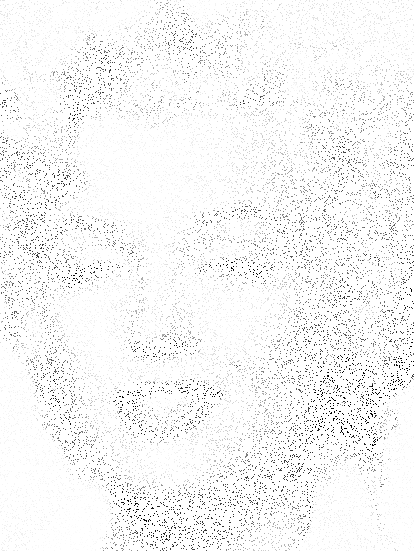
(a) input to model (32)

(b) inpainting $w$ using (32)

(c) edges $z$ using (32)

Figure 4: Solution to Problem 32. (a) shows the inpainting mask from Figure 2(b) weighted with the gray values from Figure 2(a). (b) shows the solution image $w$ and (c) the solution edge set $z$ of (32). Although the model is non-convex, visually all algorithms resulted in a similar solution. Figure 3 shows that the final objective values differ.

where $\operatorname{diag}\colon\mathbb{R}^{N}\to\mathbb{R}^{N\times N}$ puts a vector on the diagonal of a matrix. Figure 4 shows the input data, the reconstructed image, and the reconstructed edge set, for $\varepsilon=0.1$ and $\gamma=1/400$ and the number of pixel $N=551\cdot 414=228114$.

In the following, we evaluate several algorithms that use a variable metric. Let

$$g_{1}(w):=\delta_{X}(w)\text{ with }X:=\{w\in\mathbb{R}^{N}|\,w_{i}=I_{i}\ \text{if}\ c_{i}=1\}\,,\qquad g_{2}(z):=\frac{\gamma}{4\varepsilon}\|z-1\|_{2}^{2}$$

$$f(w,z):=\frac{1}{2}\left(\|\operatorname{diag}(z)(D_{1}w)\|_{2}^{2}+\|\operatorname{diag}(z)(D_{2}w)\|_{2}^{2}+\gamma\varepsilon\|Dz\|_{2}^{2}\right)\,.$$

We can apply iPiano to (8) with $x=(w,z)$ and $g(x)=(g_{1}(w),g_{2}(z))$, or block coordinate iPiano to (22) with $\mathbf{x}_{1}=w$ and $\mathbf{x}_{2}=z$.

In order to determine a suitable metric, we first compute the derivatives of $f$

$$\begin{split}\nabla_{w}f(w,z)=&\ \left(D_{1}^{\top}\operatorname{diag}(z^{2})D_{1}+D_{2}^{\top}\operatorname{diag}(z^{2})D_{2}\right)w\\ \nabla_{z}f(w,z)=&\ \left(\operatorname{diag}((D_{1}w)^{2})+\operatorname{diag}((D_{2}w)^{2})+\gamma\varepsilon D^{\top}D\right)z\,,\end{split}$$

where the squares are to be understood coordinate-wise. A feasible metric for block coordinate variable metric iPiano (BC-VM-iPiano) must satisfy (24). Therefore, for the $w$-update step ($z$ is fixed), we require $A_{n,w}$ (the metric w.r.t. the block of $w$ coordinates) to satisfy

$$\left\langle\nabla_{w}f(w,z)-\nabla_{w}f(w^{\prime},z)-A_{n,w}(w-w^{\prime}),w-w^{\prime}\right\rangle\leq 0$$

for all $w,w^{\prime}$, which is achieved, for example, by a diagonal matrix $A_{n,w}$ given by

$$(A_{n,w})_{i,i}=\sum_{j=1}^{N}|\left(D_{1}^{\top}\operatorname{diag}(z^{2})D_{1}+D_{2}^{\top}\operatorname{diag}(z^{2})D_{2}\right)_{i,j}|$$ (33)

for all $i\in\{1,\ldots,N\}$. In order to avoid numerical problems, we add a small numerical constant $10^{-9}$ to the diagonal of $A_{n,w}$. For the $z$-update ($w$ is fixed), analogously, we require $A_{n,z}$ (the metric w.r.t. the block of $z$ coordinates) to satisfy

$$\left\langle\nabla_{w}f(w,z)-\nabla_{w}f(w,z^{\prime})-A_{n,z}(z-z^{\prime}),z-z^{\prime}\right\rangle\leq 0$$

for all $z,z^{\prime}$, which is achieved, for example, by a diagonal matrix $A_{n,z}$ given by

$$(A_{n,z})_{i,i}=\sum_{j=1}^{N}|\left(\operatorname{diag}((D_{1}w)^{2})+\operatorname{diag}((D_{2}w)^{2})+\gamma\varepsilon D^{\top}D\right)_{i,j}|$$ (34)

for all $i\in\{1,\ldots,N\}$. Note that compared to (24) the metric contains the scaling $L_{n,w}$ and $L_{n,z}$, respectively. For constant step size schemes ($A_{n,w}=A_{n,z}=\mathrm{id}$) we use $L_{w}\leq 8$ and $L_{z}\leq 2+8\gamma\varepsilon$.

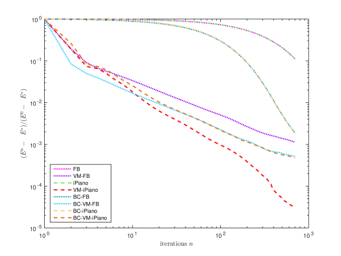
Figure 3: Number of iterations vs. relative objective value for solving (32). The performance is significantly improved for methods that take a variable metric into account. Intuitively, this means that the coordinates of the optimization variable are irregularly scaled along the iterations. The variable metric version of iPiano shows the best performance.

Besides BC-VM-iPiano, we test forward–backward splitting (FB) with constant step size scheme $\alpha=2/\max(L_{w},L_{z})$, block coordinate forward–backward splitting (BC-FB) with step sizes $\alpha_{w}=2/L_{w}$ and $\alpha_{z}=2/L_{z}$ (this method is also known as PALM [12]), variable metric forward–backward splitting (BC-FB) with the metric (33) and (34) as a composed diagonal matrix, block coordinate variable metric forward–backward splitting (BC-VM-FB) with the metric (33) and (34), iPiano (iPiano) with constant step size scheme $\alpha=2(1-\beta)/\max(L_{w},L_{z})$, block coordinate iPiano (BC-iPiano) with constant step size scheme $\alpha_{w}=2(1-\beta)/L_{w}$ and $\alpha_{z}=2(1-\beta)/L_{z}$, variable metric iPiano (VM-iPiano) with the metric (33) and (34) as a composed diagonal matrix, and block coordinate variable metric iPiano (BC-VM-iPiano) with the metric (33) and (34). For all methods that incorporate an inertial parameter, it is set to $\beta=0.7$.

The metric that is used for BC-FB and VM-iPiano is actually not feasible, as (33) and (34) are not sufficient to guarantee that the metric induces a quadratic majorizer to the function $f$ (cf. (10)). The gradient is not linear with respect to both coordinates. The gradient is linear only if one coordinate is fixed. Nevertheless, in our practical experiments, the methods converged. In future work, we want to analyze if this inaccuracy can be compensated by making use of relative error conditions, which are not yet incorporated into the algorithms.

We solve problem (32) with all methods up to 1000 iterations and define $E^{*}$ as the minimal objective value that is achieved among all methods. Let $E^{0}$ be the initial value. Figure 3 plots the decrease of the relative objective value $(E^{n}-E^{*})/(E^{0}-E^{*})$ along the iterations ${n}$ on a logarithmic scale on both axes.

The performance of FB and iPiano are nearly identical as they do not explore the different scaling of $w$- and $z$-coordinates, unlike BC-FB and BC-iPiano. As both block coordinates seem to “live” on a different scale, block coordinate methods are favorable. However, as the immense performance speed up of the variable metric methods shows the irregular scaling happens to be present also among different $w$-coordinates, respectively, $z$-coordinates. Throughout the experiments, we have noticed that optimization problems where regularization (like smoothness between pixels) is important, inertial methods seem to perform slightly better in general. For this experiment variable metric iPiano shows the best performance and sets the value for $E^{*}$, the lowest objective value among all methods after 1000 iterations. Note that the computational cost per iterations is nearly the same for all methods.

7 Conclusion

In this paper, we presented a convergence analysis for abstract inexact generalized descent methods based on the KL-inequality that unifies and generalizes the analysis in Attouch et al. [5], Frankel et al. [23], Ochs et al. [48], Bolte and Pauwels [11], and several other more explicit algorithms. The novel convergence theorem allows for more flexibility in the design of algorithms. More in detail, algorithms that imply a descent on a proper lower semi-continuous parametric function and satisfy a certain flexible relative error condition are considered. The parametric function can be seen as an objective function that may vary along the iterations. The gained flexibility is used to formulate a variable metric version of iPiano (an inertial forward–backward splitting-like method). Moreover, thanks to usage of a generic distance measure in the abstract convergence theorem, we obtain a block coordinate variable metric version of iPiano almost for free. Finally, the algorithms are shown to perform well on the practical problem of image compression using a Mumford–Shah-like regularization.

As future work, we will investigate whether the gained flexibility can be used, for example, to prove the convergence of (inertial) Bregman proximal descent methods with Bregman functions that are not required to be strongly convex or to have a Lipschitz continuous gradient.

Appendix A Appendix

A.1 Relation to algorithms with analogue convergence guarantees

In recent works, the convergence analysis of algorithms for non-smooth non-convex optimization problems often follows the lines of the proof methodology suggested in [12], i.e., the convergence is explicitly verified, although it suffices to verify the abstract conditions in [5]. In the following, for several such algorithms, the relation to the abstract conditions in [5, 23, 48] and Assumption H is shown. For [35, 37, 40], the generalizations of our paper are necessary to cast them into the abstract framework. Note that we do not provide an exhaustive list of examples. Most of the algorithms mentioned in the introduction fall into our unifying abstract setting.

Relation to PALM [12].

In [12], the general proof methodology is introduced. Thanks to a uniformization result of the KL-inequality, which we also use in this paper (see Lemma 4), the convergence proof was simplified compared to [5]. [12, Lemma 3(i)] verifies (ABS13-H1), [12, Lemma 4] shows (ABS13-H2), and [12, Lemma 5(i)] contains the continuity statement (ABS13-H3).

Relation to [15].

An inertial algorithm for the sum of two non-convex functions was proposed in this paper. The setting is slightly more general than [48] as the non-smooth part of the objective is allowed to be non-convex. The proximal subproblems are formulated with respect to Bregman distances that are required to be strongly convex and with Lipschitz continuous gradient, which provides a lower and upper bound in the Euclidean metric for the Bregman distance terms. The proof of convergence is, hence, analogue to [48]. However, unlike in [48], the sufficient decrease condition uses $d_{{n}}=\|x^{{n+1}}-x^{{n}}\|_{2}$ instead of $\|x^{{n}}-x^{{n-1}}\|_{2}$. Both conditions obviously fall into the more general set of conditions in Assumption H. The conditions in Assumption H are verified in [15, (H1)–(H3) on page 13] in analogy to (OCBP14-H1)–(OCBP14-H3) for which we provide the details in Section 3.1.

Relation to [35].

A Douglas–Rachford splitting algorithm for solving non-smooth non-convex problems of the form

$$\min_{x\in\mathbb{R}^{N}}\,f(x)+g(x)\,,$$ (35)

where $f$ has Lipschitz continuous gradient and $g$ is proper lower semi-continuous, is proposed. The algorithm generates sequences $(x^{{n}})_{{n}\in\mathbb{N}}$, $(y^{{n}})_{{n}\in\mathbb{N}}$, and $(z^{{n}})_{{n}\in\mathbb{N}}$ according to the following update scheme: $(\gamma>0)$

$$\begin{split}y^{{n+1}}\in&\ \underset{y}{\operatorname{argmin}}\,f(y)+\frac{1}{2\gamma}\|y-x^{{n}}\|_{2}^{2}\\ z^{{n+1}}\in&\ \underset{z}{\operatorname{argmin}}\,g(z)+\frac{1}{2\gamma}\|2y^{{n+1}}-x^{{n}}-z\|_{2}^{2}\\ x^{{n+1}}=&\ x^{{n}}+(z^{{n+1}}-y^{{n+1}})\end{split}$$

The global convergence of the whole sequence $((y^{{n}},z^{{n}},x^{{n}}))_{{n}\in\mathbb{N}}$ is shown in [35, Theorem 2] for certain values of $\gamma>0$, and is based on a descent property of the merit function

$$\mathfrak{D}_{\gamma}(y,z,x):=f(y)+g(z)-\frac{1}{2\gamma}\|y-z\|_{2}^{2}+\left\langle x-y,z-y\right\rangle\,.$$

During the proof, which they tailored to their method, the abstract conditions in Assumption H are verified. (H1) is verified in [35, Eq. (23)] with some constant $a>0$ for the function $\mathfrak{D}_{\gamma}$ using $d^{{n}}:=\|y^{{n+1}}-y^{{n}}\|_{2}$

$$\mathfrak{D}_{\gamma}(y^{{n+1}},z^{{n+1}},x^{{n+1}})+a\|y^{{n+1}}-y^{{n}}\|_{2}^{2}\leq\mathfrak{D}_{\gamma}(y^{{n}},z^{{n}},x^{{n}})\,,$$

(H2) is established in [35, Eq. (28)] for some $b>0$,

$$\operatorname{dist}(0,\partial\mathfrak{D}_{\gamma}(y^{{n}},z^{{n}},x^{{n}}))\leq b\|y^{{n+1}}-y^{{n}}\|_{2}\,,$$

using $I:=\{0\}$, $\theta_{0}=1$, $b_{{n}}\equiv 1$, $\varepsilon_{{n}}\equiv 0$, and (H3) is proved by assuming the existence of a cluster point and the $\mathfrak{D}_{\gamma}$-attentive convergence from [35, Eq. (25)–(27)]. The distance condition (H4) is asserted by [35, Eq. (22),(10)] and the relation in the $x$-update step. (H5) is obviously satisfied, since we are in a setting with constant parameters. Therefore, we can apply our Theorem 10 to prove the same convergence results as in [35, Theorem 2]: $(y^{{n}})_{{n}\in\mathbb{N}}$ converges and, using the same equations that realize the distance condition, convergence of $(z^{{n}})_{{n}\in\mathbb{N}}$ and $(x^{{n}})_{{n}\in\mathbb{N}}$ can be concluded.

Relation to [37].

In a similar way to [35], the proximal ADMM proposed in [37] can be cast into our framework. The goal is to solve the following problem:

$$\min_{x\in\mathbb{R}^{N}}\,h(x)+P(\mathcal{M}x)\,,$$

with a linear mapping $\mathcal{M}$, a proper lower semi-continuous function $P$, and a twice continuously differentiable function $h$ with bounded Hessian. The sufficient decrease condition is proved for the Lagrange function

$$L_{\beta}(x,y,z)=h(x)+P(y)-\left\langle z,\mathcal{M}x-y\right\rangle+\frac{\beta}{2}\|\mathcal{M}x-y\|_{2}^{2}$$

in [37, Eq. (36)] with $d^{{n}}:=\|x^{{n+1}}-x^{{n}}\|_{2}$, and some $a>0$. Different from the analysis in [35], where the relative error condition is explicit, it is implicit in [37]. The condition (H2) is verified in [37, Eq. (35)] for some $b>0$, $b_{{n}}\equiv 1$, $\varepsilon_{{n}}\equiv 0$, $I=\{1\}$ and $\theta_{1}=1$. The condition (H3) is proved in [37, Theorem 2(i)]. The distance condition (H4) follows directly from [37, Eq. (14),(15)], and (H5) is again obviously satisfied.

Relation to [40].

A very general multi-step forward–backward scheme is proposed to solve problems of the setting of (35). The main update step is a forward–backward step, executed at an extrapolated point with gradient direction evaluated at another extrapolated point. Both of these extrapolations allow for a linear combination (possibly different ones) of finitely many preceding step directions. Global convergence and a finite length property are proved in [40, Theorem 2.2] explicitly for this algorithm for the sequence $(x^{{n}})_{{n}\in\mathbb{N}}$ and $(z^{{n}})_{{n}\in\mathbb{N}}$ with $z^{{n}}=(x^{{n}},x^{{n-1}},\ldots,x^{n-s+1})$ for some $s\in\mathbb{N}$. The statements that establishes the conditions in Assumption H are collected in [40, (R.1)–(R.3)] in the supplementary material. The proof idea follows the concepts of the proof of iPiano [48]. The arising Lyapunov function and the product space is naturally generalized to the number of terms used in the linear combinations of the extrapolations.

References

- [1] P. Absil, R. Mahony, and B. Andrews. Convergence of the iterates of descent methods for analytic cost functions. SIAM Journal on Optimization, 16(2):531–547, Jan. 2005.
- [2] L. Ambrosio and V. Tortorelli. Approximation of functionals depending on jumps by elliptic functionals via -convergence. Communications on Pure and Applied Mathematics, 43:999–1036, 1990.
- [3] H. Attouch and J. Bolte. On the convergence of the proximal algorithm for nonsmooth functions involving analytic features. Mathematical Programming, 116(1):5–16, June 2009.
- [4] H. Attouch, J. Bolte, P. Redont, and A. Soubeyran. Proximal alternating minimization and projection methods for nonconvex problems: An approach based on the Kurdyka-Łojasiewicz inequality. Mathematics of Operations Research, 35(2):438–457, May 2010.
- [5] H. Attouch, J. Bolte, and B. Svaiter. Convergence of descent methods for semi-algebraic and tame problems: proximal algorithms, forward–backward splitting, and regularized Gauss–Seidel methods. Mathematical Programming, 137(1-2):91–129, 2013.
- [6] A. Auslender. Asymptotic properties of the Fenchel dual functional and applications to decomposition problems. Journal of Optimization Theory and Applications, 73(3):427–449, June 1992.
- [7] J. Bolte, P. Combettes, and J.-C. Pesquet. Alternating proximal algorithm for blind image recovery. In International Conference on Image Processing (ICIP), pages 1673–1676, Honk Kong, China, Sept. 2010.
- [8] J. Bolte, A. Daniilidis, and A. Lewis. The Łojasiewicz inequality for nonsmooth subanalytic functions with applications to subgradient dynamical systems. SIAM Journal on Optimization, 17(4):1205–1223, Dec. 2006.
- [9] J. Bolte, A. Daniilidis, A. Lewis, and M. Shiota. Clarke subgradients of stratifiable functions. SIAM Journal on Optimization, 18(2):556–572, 2007.
- [10] J. Bolte, A. Daniilidis, A. Ley, and L. Mazet. Characterizations of Łojasiewicz inequalities: subgradient flows, talweg, convexity. Transactions of the American Mathematical Society, 362:3319–3363, 2010.
- [11] J. Bolte and E. Pauwels. Majorization-minimization procedures and convergence of SQP methods for semi-algebraic and tame programs. Mathematics of Operations Research, Jan. 2016.
- [12] J. Bolte, S. Sabach, and M. Teboulle. Proximal alternating linearized minimization for nonconvex and nonsmooth problems. Mathematical Programming, 146(1-2):459–494, 2014.
- [13] S. Bonettini, I. Loris, F. Porta, M. Prato, and S. Rebegoldi. On the convergence of variable metric line-search based proximal-gradient method under the Kurdyka-Lojasiewicz inequality. ArXiv e-prints, May 2016. arXiv:1605.03791.
- [14] R. I. Bot and E. R. Csetnek. An inertial Tseng’s type proximal algorithm for nonsmooth and nonconvex optimization problems. Journal of Optimization Theory and Applications, pages 1–17, Mar. 2015.
- [15] R. I. Bot, E. R. Csetnek, and S. László. An inertial forward–backward algorithm for the minimization of the sum of two nonconvex functions. EURO Journal on Computational Optimization, pages 1–23, Aug. 2015.
- [16] L. M. Bregman. The relaxation method of finding the common point of convex sets and its application to the solution of problems in convex programming. USSR Computational Mathematics and Mathematical Physics, 7(3):200–217, 1967.
- [17] R. Chill and M. Jendoubi. Convergence to steady states in asymptotically autonomous semilinear evolution equations. Nonlinear Analysis: Theory, Methods & Applications, 53(7):1017–1039, June 2003.
- [18] E. Chouzenoux, J.-C. Pesquet, and A. Repetti. Variable metric forward–backward algorithm for minimizing the sum of a differentiable function and a convex function. Journal of Optimization Theory and Applications, Nov. 2013.
- [19] E. Chouzenoux, J.-C. Pesquet, and A. Repetti. A block coordinate variable metric forward–backward algorithm. Journal of Global Optimization, pages 1–29, Feb. 2016.
- [20] P. Combettes and B. V. u. Variable metric quasi-Fejér monotonicity. Nonlinear Analysis: Theory, Methods & Applications, 78:17–31, Feb. 2013.
- [21] P. Combettes and B. V. u. Variable metric forward–backward splitting with applications to monotone inclusions in duality. Optimization, 63(9):1289–1318, Sept. 2014.
- [22] L. V. den Dries. Tame topology and -minimal structures. 150 184. Cambridge University Press, 1998.
- [23] P. Frankel, G. Garrigos, and J. Peypouquet. Splitting methods with variable metric for Kurdyka–Łojasiewicz functions and general convergence rates. Journal of Optimization Theory and Applications, 165(3):874–900, Sept. 2014.
- [24] I. Galic, J. Weickert, M. Welk, A. Bruhn, A. Belyaev, and H.-P. Seidel. Towards PDE-based image compression. In N. Paragios, O. D. Faugeras, T. Chan, and C. Schnörr, editors, VLSM, volume 3752 of Lecture Notes in Computer Science, pages 37–48. Springer, 2005.
- [25] B. Gao, X. Liu, X. Chen, and Y. Yuan. On the Łojasiewicz exponent of the quadratic sphere constrained optimization problem. ArXiv e-prints, Nov. 2016. arXiv: 1611.08781.
- [26] L. Grippof and M. Sciandrone. Globally convergent block-coordinate techniques for unconstrained optimization. Optimization Methods and Software, 10(4):587–637, Jan. 1999.
- [27] A. Haraux and M. Jendoubi. Convergence of solutions of second-order gradient-like systems with analytic nonlinearities. Journal of Differential Equations, 144(2):313–320, Apr. 1998.
- [28] S. Hosseini. Convergence of nonsmooth descent methods via Kurdyka–Łojasiewicz inequality on Riemannian manifolds. Technical Report 1523, Institut für Numerische Simulation, Rheinische Friedrich–Wilhelms–Universität Bonn, Bonn, Germany, Nov. 2015.
- [29] S.-Z. Huang and P. Takáč. Convergence in gradient-like systems which are asymptotically autonomous and analytic. Nonlinear Anal., 46(5):675–698, Nov. 2001.
- [30] D. R. Hunter and K. Lange. A tutorial on MM algorithms. Journal of the American Statistical Association, 58(1):30–37, 2004.
- [31] A. Iusem, T. Pennanen, and B. Svaiter. Inexact variants of the proximal point algorithm without monotonicity. SIAM Journal on Optimization, 13(4):1080–1097, Jan. 2003.
- [32] K. Kurdyka. On gradients of functions definable in o-minimal structures. Annales de l’institut Fourier, 48(3):769–783, 1998.
- [33] K. Kurdyka and A. Parusiński. -stratification of subanalytic functions and the Łojasiewicz inequality. C. R. Acad. Paris, 318:129–133, 1994.
- [34] C. Lageman. Pointwise convergence of gradient-like systems. Mathematische Nachrichten, 280(13-14):1543–1558, Oct. 2007.
- [35] G. Li and T. Pong. Douglas–Rachford splitting for nonconvex optimization with application to nonconvex feasibility problems. Mathematical Programming, 159(1-2):371–401, Sept. 2016.
- [36] G. Li and T. Pong. Calculus of the exponent of Kurdyka–Łojasiewicz inequality and its applications to linear convergence of first-order methods. Foundations of Computational Mathematics, pages 1–34, Aug. 2017.
- [37] G. Li and T. K. Pong. Global convergence of splitting methods for nonconvex composite optimization. SIAM Journal on Optimization, 25(4):2434–2460, Jan. 2015.
- [38] G. Li and T. K. Pong. Peaceman–Rachford splitting for a class of nonconvex optimization problems. arXiv:1507.00887 [cs, math], July 2015. arXiv: 1507.00887.
- [39] H. Li and Z. Lin. Accelerated proximal gradient method for nonconvex programming. In C. Cortes, N. D. Lawrence, D. D. Lee, M. Sugiyama, and R. Garnett, editors, Advances in Neural Information Processing Systems (NIPS), pages 379–387. Curran Associates, Inc., 2015.
- [40] J. Liang, J. Fadili, and G. Peyré. A multi-step inertial forward–backward splitting method for non-convex optimization. In D. Lee, M. Sugiyama, U. Luxburg, I. Guyon, and R. Garnett, editors, Advances in Neural Information Processing Systems (NIPS), pages 4035–4043. Curran Associates, Inc., 2016.
- [41] S. Łojasiewicz. Une propriété topologique des sous-ensembles analytiques réels. In Les Équations aux Dérivées Partielles, pages 87–89, Paris, 1963. Éditions du centre National de la Recherche Scientifique.
- [42] S. Łojasiewicz. Sur la géométrie semi- et sous- analytique. Annales de l’institut Fourier, 43(5):1575–1595, 1993.
- [43] M. Mainberger and J. Weickert. Edge-based image compression with homogeneous diffusion. In X. Jiang and N. Petkov, editors, Computer Analysis of Images and Patterns, volume 5702 of Lecture Notes in Computer Science, pages 476–483. Springer Berlin Heidelberg, 2009.
- [44] B. Merlet and M. Pierre. Convergence to equilibrium for the backward Euler scheme and applications. Communications on Pure and Applied Analysis, 9(3):685–702, Jan. 2010.
- [45] Y. Nesterov. Introductory lectures on convex optimization: A basic course, volume 87 of Applied Optimization. Kluwer Academic Publishers, Boston, MA, 2004.
- [46] D. Noll. Convergence of non-smooth descent methods using the Kurdyka–Łojasiewicz inequality. Journal of Optimization Theory and Applications, 160(2):553–572, Sept. 2013.
- [47] P. Ochs. Long term motion analysis for object level grouping and nonsmooth optimization methods. PhD thesis, Albert-Ludwigs-Universität Freiburg, Mar 2015.
- [48] P. Ochs, Y. Chen, T. Brox, and T. Pock. iPiano: Inertial proximal algorithm for non-convex optimization. SIAM Journal on Imaging Sciences, 7(2):1388–1419, 2014.
- [49] P. Ochs, A. Dosovitskiy, T. Brox, and T. Pock. On iteratively reweighted algorithms for nonsmooth nonconvex optimization in computer vision. SIAM Journal on Imaging Sciences, 8(1):331–372, 2015.
- [50] T. Pock and S. Sabach. Inertial proximal alternating linearized minimization (iPALM) for nonconvex and nonsmooth problems. SIAM Journal on Imaging Sciences, 9(4):1756–1787, Jan. 2016.
- [51] B. T. Polyak. Some methods of speeding up the convergence of iteration methods. USSR Computational Mathematics and Mathematical Physics, 4(5):1–17, 1964.
- [52] R. T. Rockafellar and R. J.-B. Wets. Variational Analysis, volume 317. Springer Berlin Heidelberg, Heidelberg, 1998.
- [53] L. Simon. Asymptotics for a class of non-linear evolution equations with applications to geometric problems. Annals of Mathematics, 118(3):525–571, 1983.
- [54] M. Solodov and B. Svaiter. A hybrid approximate extragradient–proximal point algorithm using the enlargement of a maximal monotone operator. Set-Valued Analysis, 7(4):323–345, Dec. 1999.
- [55] M. Solodov and B. Svaiter. A hybrid projection-proximal point algorithm. Journal of Convex Analysis, 6(1):50–70, 1999.
- [56] M. Solodov and B. Svaiter. A unified framework for some inexact proximal point algorithms. Numerical Functional Analysis and Optimization, 22(7-8):1013–1035, Nov. 2001.
- [57] A. J. Wilkie. Model completeness results for expansions of the ordered field of real numbers by restricted Pfaffian functions and the exponential function. Journal of the American Mathematical Society, 9(4):1051–1094, 1996.
- [58] S. Zavriev and F. Kostyuk. Heavy-ball method in nonconvex optimization problems. Computational Mathematics and Modeling, 4(4):336–341, 1993.