Dynamics of dipoles and vortices in nonlinearly-coupled three-dimensional field oscillators

Abstract

The dynamics of a pair of harmonic oscillators (HOs) represented by three-dimensional fields coupled by a repulsive cubic nonlinearity is investigated through direct simulations of the respective field equations, and with the help of the finite-mode Galerkin approximation (GA), which represents the two interacting fields by a superposition of $3+3$ HO p-wave eigenfunctions with orbital and magnetic quantum numbers $l=1$ and $m=1,0,-1$. The system can be implemented in binary Bose-Einstein condensates, demonstrating a potential of the atomic condensates for emulating various complex modes predicted by classical field theories, First, the GA very accurately predicts a broadly degenerate set of the system’s ground states in the p-wave manifold, in the form of complexes built of a dipole coaxial with another dipole or vortex, as well as complexes built of mutually orthogonal dipoles. Next, pairs of non-coaxial vortices and/or dipoles, including pairs of mutually perpendicular vortices, develop remarkably stable dynamical regimes, which feature periodic exchange of the angular momentum and periodic switching between dipoles and vortices. For a moderately strong nonlinearity, simulations of the coupled field equations agree very well with results produced by the GA, demonstrating that the dynamics is accurately spanned by the set of six modes limited to $l=1$.

I Introduction

The study of diverse complex three-dimensional (3D) modes, such as spinning solitons and vortex rings vortex-rings , knots knots , hopfions hopfions , and skyrmions skyrmions is one of central topics in the classical field theory review . In addition to the well-known applications of skyrmions to low-energy hadron physics hadrons , states approximated by the field-theory modes can be identified in ferromagnets and ferroelectrics ferro , superconductors super , and semiconductors semi .

An exceptionally clean and well-controlled implementation of various modes predicted in the field theory is offered by atomic Bose-Einstein condensates (BECs). In particular, the possibility of the creation of BEC skyrmions was predicted in a number of settings BEC-skyrmions and realized experimentally skyrmion-exper . Also predicted were settings appropriate for the creation of atomic knots BEC-knots and hopfions BEC-hopfion , and the experimental creation of monopoles was recently reported in Ref. monopole-exper .

This topic is closely related to the general problem of the creation of 2D and 3D self-trapped modes in nonlinear media (often considered as solitons), which also finds many physically relevant ramifications general-reviews , RMP , especially in nonlinear optics and matter-wave dynamics in BECs. In addition to the great significance to fundamental studies in these fields, 2D optical solitons may be used as bit carriers in all-optical data-processing schemes Wagner , and 3D matter-wave solitons are expected to provide a basis for precise interferometry interferometry .

The objective of this work is to demonstrate that a 3D two-component system, which can be readily implemented in BEC, makes it possible to create new nontrivial bound states and robust dynamical regimes, built of coaxial or mutually perpendicular dipole modes or vortices in the two components, that are of definite interest as field-theory modes, and, simultaneously, suggest novel possibilities for the experimental emulation of the field-theory settings in atomic BEC. Although the overall 3D nonlinear-field dynamics seems complex enough (remaining regular, rather then getting chaotic), a remarkable fact is that it can be very accurately represented by a six-mode Galerkin approximation (GA), which, in turn, admits an essentially analytical investigation. This finding suggests that the projection onto an appropriately chosen GA may be useful in other nonlinear field-theory models too.

Getting back to the introduction into the general topic, it is relevant to mention that the creation of multidimensional solitons is often complicated by the fact that such states, usually supported by the cubic self-focusing nonlinearity, are subject to instability caused by the wave collapse (critical and supercritical collapse in 2D and 3D, respectively) collapse . Multidimensional vortex solitons, alias vortex rings, in cubic media are vulnerable to a still stronger splitting instability induced by modulational perturbations in the azimuthal direction general-reviews . These instabilities may be suppressed by means of periodic potentials (lattices), as was predicted theoretically lattice and demonstrated in the experiment photorefr ; very recently, it was also predicted that the spin-orbit coupling can stabilize 2D Fukuoka and 3D HP solitons in two-component systems.

Such physical media are modeled by the non-relativistic nonlinear Schrödinger equation, alias Gross-Pitaevskii equation (GPE) Pit , for the corresponding photonic or atomic mean-field wave function $\Phi\left(\mathbf{r},t\right)$, where $\mathbf{r}=(x,y,z)$ and $t$ are appropriately scaled spatial coordinates and time:

$$i\frac{\partial\Phi}{\partial t}=-\nabla^{2}\Phi+U\left(\mathbf{r}\right)\Phi+\sigma|\Phi|^{2}\Phi.$$ (1)

In this equation, $\nabla^{2}$ is the 3D Laplacian, $U\left(\mathbf{r}\right)$ is the trapping potential, and $\sigma=-1$ or $+1$ corresponds to the self-focusing or defocusing (repulsive) sign of the cubic interaction. In particular, in the case of axially symmetric potentials (including spherically isotropic ones), $U=U\left(\rho,z\right)$, where $\left(\rho,z,\varphi\right)$ is the set of cylindrical coordinates, Eq. (1) admits vortical modes in the form of

$$\Phi=\exp\left(-i\mu t+il\varphi\right)u(\rho,z),$$ (2)

with real chemical potential $\mu$, integer vorticity $l$, and real amplitude function $u\left(\rho,z\right)$ satisfying the stationary equation,

$$\mu u=-\left(\frac{\partial^{2}}{\partial\rho^{2}}+\frac{1}{\rho}\frac{\partial}{\partial\rho}+\frac{\partial^{2}}{\partial z^{2}}-\frac{l^{2}}{\rho^{2}}\right)u+U\left(\rho,z\right)u+\sigma u^{3}.$$ (3)

A novel approach for the creation of self-trapped modes was proposed in Ref. ICFO : A spatially inhomogeneous repulsive cubic nonlinearity, whose local strength in the space of dimension $D$ grows from the center to periphery faster than $r^{D}$ ($r$ is the radial coordinate), supports extremely robust and diverse families of solitons, multipoles, fundamental and composite solitary vortices, and hopfions for $D=1,2,3$ further . This type of the nonlinearity modulation belongs to the general class of the nonlinear pseudopotentials, which can be induced by various techniques in optics for $D=1,2$, and in BEC for $D=3$ too RMP .

On the other hand, it was demonstrated in detail theoretically that the usual 2D and 3D settings, which combine spatially uniform cubic self-repulsion and an isotropic harmonic-oscillator (HO) trapping potential, readily give rise to various bound states, including trapped vortices vortices as well as vortex clusters and dipoles vort-clusters . The formation of vortices in optics and BEC was reported in many experimental works vort-exper , see also review vort-rev . The stability of the vortices in these settings is essentially secured by the fact that the repulsive nonlinearity does not give rise to modulational instability.

Multi-component BECs with repulsive self- and cross-interactions (usually, they are realized as mixtures of different hyperfine atomic states of the same species) may also give rise to stable vortices 2comp-vort and, furthermore, to the above-mentioned matter-wave skyrmions BEC-skyrmions ; skyrmion-exper and monopoles monopole-exper . Further, the studies of two-component systems suggest that two identical 3D GPEs coupled by the repulsive interaction, each with an isotropic HO trapping potential, may be used as a simple model for the analysis of nontrivial dynamical regimes, such as interaction of non-coaxial (or, more specifically, mutually perpendicular) trapped vortices or dipoles initially created in the two wave fields. This possibility was recently proposed in Ref. arxiv were stable vortices having orthogonal vortex lines and trapped in a HO trap were found. If initially the modes deviate from the stationary state, the nonlinear repulsive interactions lead to smooth dynamics representing torque-free precession with nutations. The model was studied under the condition that the inter-species repulsion was weaker than the self-repulsion in each component. In this case, it was concluded that the system is robust with respect to variation of parameters.

In the present work we address a system of two GPEs which is dominated by intra-species repulsion, while the intra-species self-interactions may be neglected. We predict experimentally observable stationary and dynamical modes by means of systematic simulations and, in parallel, making use of the above-mentioned six-mode GA. The approach developed here is similar to its well-known applications of the GA in hydrodynamics GA , projecting the coupled GPEs for two mean-field wave functions onto the truncated dynamical system. The six-mode truncation approximates each wave function by a combination of three p-wave eigenfunctions of the 3D HO, with orbital quantum number $l=1$ and magnetic quantum numbers $m=-1,0,+1$, assuming that the axes which define the two triplets of the eigenfunctions are mutually perpendicular. The accuracy provided by the GA turns out to be surprisingly high, provided that the nonlinear interaction is not too strong (at certain threshold of nonlinear interaction strength a deviation from the GA is observed due to generation of components with $l>1$). In particular, fixed points (FPs) of the GA provide for a very good approximation for quasi-stationary states of the coupled GPE system. Taking sets of non-coaxial dipoles or vortices in the two wave fields as initial states, their nonlinear interaction leads, in the framework of the GPEs and GA alike, to remarkably robust dynamical regimes, which are characterized by a periodic exchange of the angular momentum between the two field components and a periodic switch of their structure, with the dipoles transforming into vortices and vice versa.

The model and GA are introduced in Sec. II, which is followed by the analysis of the GA’s FPs in Sec. III. In the same section, we also produce (energy-degenerate) ground states (GSs) of the coupled GPEs in the p-wave manifold, which are very accurately predicted by the FPs of the GA. In Sec. IV we present systematic results for the dynamics of pairs of non-coaxial nonlinearly coupled dipoles and/or vortices. The paper is concluded by Sec. V.

II The model and the Galerkin approximation

The scaled form of the underlying system of the coupled 3D GPEs with the repulsive interaction between the two wave functions, $\Phi$ and $\Psi$, and the isotropic HO potential, represented by terms $\sim r^{2}$, is

$$i\frac{\partial\Phi}{\partial t} = -\nabla^{2}\Phi+r^{2}\Phi+|\Psi|^{2}\Phi,$$ (4)

$$i\frac{\partial\Psi}{\partial t} = -\nabla^{2}\Psi+r^{2}\Psi+|\Phi|^{2}\Psi.$$ (5)

Unlike Ref. arxiv , we here consider the system with negligible self-repulsion of each component in comparison with the repulsive interaction between them. In the BEC experiment, this situation may be achieved using the Feshbach resonance (FR) induced by external magnetic field to strengthen the inter-component repulsion Feshbach+rf ; Feshbach2 , thus making this interaction much stronger than the intra-component interactions. The effect of the FR may be additionally enhanced if applied to atomic states “dressed” by a radio-frequency field Feshbach+rf ; Shlyap ). In particular, it was demonstrated experimentally Feshbach2 that the FR can make the scattering length accounting for the repulsion between atomic states of ⁸⁷Rb with quantum numbers $\left|F=1,m_{F}=+1\right\rangle$ and $\left|F=2,m_{F}=-1\right\rangle$, at magnetic field $9.10$ G, larger by a factor $\simeq 15$ than the scattering length which represents the intra-component self-repulsion, cf. Ref. Australia . In fact, simulations of equations obtained from Eqs. (4), (5) by adding self-repulsion terms, i.e., $\epsilon|\Phi|^{2}\Phi$ and $\epsilon|\Psi|^{2}\Psi$, respectively produce results(not shown here in detail) which are qualitatively similar to those presented in the current work for $\epsilon=0$. Only quantitative characteristics will be fifferent such as duration of nutations as well as the duration of the total round trip. Pure numerical examples with SPM included for a pair of vortices are presented in arxiv .

Equations (4) and (5) conserve two norms,

$$N_{\Phi}=\int\left|\Phi(\mathbf{r}))\right|^{2}d\mathbf{r},\qquad N_{\Psi}=\int\left|\Psi(\mathbf{r})\right|^{2}d\mathbf{r},$$ (6)

the total vectorial angular momentum, $\mathbf{M}=\mathbf{M}_{\Phi}+\mathbf{M}_{\Psi}$ where

$$\mathbf{M}_{\Phi}=-i\int\Phi^{\ast}\left(\mathbf{r}\times\nabla\right)\Phi\,d\mathbf{r},\qquad\mathbf{M}_{\Psi}=-i\int\Psi^{\ast}\left(\mathbf{r}\times\nabla\right)\Psi\,d\mathbf{r},$$ (7)

and the Hamiltonian,

$$H=\int\left[\left|\nabla\Phi\right|^{2}+\left|\nabla\Psi\right|^{2}+r^{2}\left(|\Phi|^{2}+|\Psi|^{2}\right)\right]\,d\mathbf{r}+E_{\mathrm{int}},$$ (8)

which includes the interaction energy,

$$E_{\mathrm{int}}=\int\left|\Phi(\mathbf{r})\right|^{2}\left|\Psi(\mathbf{r})\right|^{2}\,d\mathbf{r}.$$ (9)

Note that, for stationary vortical modes, with

$$\left\{\Phi,\Psi\right\}=\exp\left(-i\mu t+il\varphi\right)\left\{u(\rho,z),v\left(\rho,z\right)\right\}$$ (10)

(cf. Eq. (2)), it follows from Eq. (7) that the absolute value of the total angular momentum is a multiple of the norm,

$$M_{\Phi,\Psi}=lN_{\Phi,\Psi},$$ (11)

irrespective of the particular structure of modal functions $u\left(\rho,z\right)$ and $v\left(\rho,z\right)$ in Eq. (10).

As said above, the GA represents the two wave functions, $\Phi$ and $\Psi$, as superpositions of three p-wave HO eigenstates, $\left(1/\sqrt{C_{lm}}\right)re^{-r^{2}/2}Y_{l}^{m}\left(\mathbf{r}\right)$, where $Y_{l}^{m}$ are spherical harmonics (written in terms of the Cartesian coordinates; recall that $r=\sqrt{x^{2}+y^{2}+z^{2}}$) with quantum numbers $l=1$, $m=1,0,-1$, and normalization constants $C_{lm}=\int\mathbf{dr~{}}r^{2}e^{-r^{2}}\left|Y_{l}^{m}\left(\mathbf{r}\right)\right|^{2}$. We define the GA so that the vorticity axes for the two triplets of the eigenfunctions are aligned with perpendicular coordinate directions, $z$ and $y$ (cf. Ref. arxiv ). Thus we use the following Ansätze, in which the normalized HO eigenfunctions are substituted in their explicit forms, and $a_{1,0,-1}(t)$ and $b_{1,0,-1}(t)$ are the expansion amplitudes:

$$\Phi\left(\mathbf{r},t\right) = \frac{1}{\pi^{3/4}}e^{-5it}re^{-r^{2}/2}\left[a_{1}(t)\frac{x+iy}{r}+\sqrt{2}a_{0}(t)\frac{z}{r}+a_{-1}(t)\frac{x-iy}{r}\right],$$ (12)

$$\Psi\left(\mathbf{r},t\right) = \frac{1}{\pi^{3/4}}e^{-5it}re^{-r^{2}/2}\left[b_{1}(t)\frac{x-iz}{r}+\sqrt{2}b_{0}(t)\frac{y}{r}+b_{-1}(t)\frac{x+iz}{r}\right].$$ (13)

Then, the evolution equations for the amplitudes are produced by the projection of the GPEs (4) and (5) onto the set of the eigenfunctions. After some algebra, the following dynamical system with six degrees of freedom is thus derived [$\tau\equiv t/\left(16\sqrt{2}\pi^{3/2}\right)$]:

$$i\frac{d{a}_{1}}{d\tau}=2|b_{0}|^{2}(2a_{1}-a_{-1})+(|b_{1}|^{2}+|b_{-1}|^{2})(3a_{1}+a_{-1})+$$

$$+a_{0}\left[b_{0}(b_{1}^{\ast}-b_{-1}^{\ast})+b_{0}^{\ast}(b_{-1}-b_{1})\right]+(a_{1}+a_{-1})(b_{1}b_{-1}^{\ast}+b_{1}^{\ast}b_{-1})-$$

$$-i\sqrt{2}\left[a_{0}(b_{-1}^{\ast}b_{1}-b_{-1}b_{1}^{\ast})+a_{-1}(b_{0}b_{-1}^{\ast}+b_{0}b_{1}^{\ast}+b_{0}^{\ast}b_{-1}+b_{0}^{\ast}b_{1})\right],$$

$$i\frac{d{a}_{0}}{d\tau}=2a_{0}(|b_{0}|^{2}+2|b_{-1}|^{2}+2|b_{1}|^{2})-2a_{0}\left(b_{1}b_{-1}^{\ast}+b_{1}^{\ast}b_{-1}\right)-$$

$$-(a_{1}-a_{-1})(b_{0}(b_{1}^{\ast}-b_{-1}^{\ast})-b_{0}^{\ast}(b_{1}-b_{-1}))-\sqrt{2}i(a_{-1}+a_{1})\left(b_{1}b_{-1}^{\ast}-b_{1}^{\ast}b_{-1}\right),$$

$$i\frac{d{a}_{-1}}{d\tau}=2|b_{0}|^{2}(2a_{-1}-a_{1})+(|b_{1}|^{2}+|b_{-1}|^{2})(3a_{-1}+a_{1})-$$

$$-a_{0}\left[b_{0}(b_{1}^{\ast}-b_{-1}^{\ast})+b_{0}^{\ast}(b_{-1}-b_{1})\right]+(a_{1}+a_{-1})(b_{1}b_{-1}^{\ast}+b_{1}^{\ast}b_{-1})+$$

$$+i\sqrt{2}\left[a_{0}(b_{-1}b_{1}^{\ast}-b_{-1}^{\ast}b_{1})+a_{1}(b_{0}b_{-1}^{\ast}+b_{0}b_{1}^{\ast}+b_{0}^{\ast}b_{-1}+b_{0}^{\ast}b_{1})\right];$$ (14)

$$i\frac{d{b}_{1}}{d\tau}=2|a_{0}|^{2}(2b_{1}-b_{-1})+(|a_{1}|^{2}+|a_{-1}|^{2})(3b_{1}+b_{-1})+$$

$$+b_{0}\left[a_{0}(a_{1}^{\ast}-a_{-1}^{\ast})+a_{0}^{\ast}(a_{-1}-a_{1})\right]+(b_{1}+b_{-1})(a_{1}a_{-1}^{\ast}+a_{1}^{\ast}a_{-1})+$$

$$+i\sqrt{2}\left[b_{0}(a_{-1}^{\ast}a_{1}-a_{-1}a_{1}^{\ast})+b_{-1}(a_{0}a_{-1}^{\ast}+a_{0}a_{1}^{\ast}+a_{0}^{\ast}a_{-1}+a_{0}^{\ast}a_{1})\right],$$

$$i\frac{d{b}_{0}}{d\tau}=2b_{0}(|a_{0}|^{2}+2|a_{-1}|^{2}+2|a_{1}|^{2})-2b_{0}\left(a_{1}a_{-1}^{\ast}+a_{1}^{\ast}a_{-1}\right)-$$

$$-(b_{1}-b_{-1})(a_{0}(a_{1}^{\ast}-a_{-1}^{\ast})-a_{0}^{\ast}(a_{1}-a_{-1}))+\sqrt{2}i(b_{-1}+b_{1})\left(a_{1}a_{-1}^{\ast}-a_{1}^{\ast}a_{-1}\right),$$

$$i\frac{d{b}_{-1}}{d\tau}=2|a_{0}|^{2}(2b_{-1}-b_{1})+(|a_{1}|^{2}+|a_{-1}|^{2})(3b_{-1}+b_{1})-$$

$$-b_{0}\left[a_{0}(a_{1}^{\ast}-a_{-1}^{\ast})+a_{0}^{\ast}(a_{-1}-a_{1})\right]+(b_{1}+b_{-1})(a_{1}a_{-1}^{\ast}+a_{1}^{\ast}a_{-1})-$$

$$-i\sqrt{2}\left[b_{0}(a_{1}^{\ast}a_{-1}-a_{-1}^{\ast}a_{1})+b_{1}(a_{0}a_{-1}^{\ast}+a_{0}a_{1}^{\ast}+a_{0}^{\ast}a_{-1}+a_{0}^{\ast}a_{1})\right].$$ (15)

It is straightforward to check that Eqs. (14) and (15) conserve the two norms, which exactly correspond to expressions (6),

$$N_{a}=|a_{-1}|^{2}+|a_{0}|^{2}+|a_{1}|^{2},\quad N_{b}=|b_{-1}|^{2}+|b_{0}|^{2}+|b_{1}|^{2},$$ (16)

and the equations can be written in the canonical Hamiltonian form

$$i\frac{da_{j}}{d\tau}=\frac{\partial H}{\partial a_{j}^{\ast}},\quad i\frac{db_{j}}{d\tau}=\frac{\partial H}{\partial b_{j}^{\ast}},$$ (17)

$j=1,0,-1$, where the conserved Hamiltonian can be cast in the following form, taking into account the definition of the norms (16):

$$H=3N_{a}N_{b}+|b_{0}|^{2}N_{a}+|a_{0}|^{2}N_{b}+$$

$$+(|a_{-1}|^{2}+|a_{1}|^{2}-2|a_{0}|^{2})(b_{1}b_{-1}^{\ast}+b_{1}^{\ast}b_{-1})+(|b_{-1}|^{2}+|b_{1}|^{2}-2|b_{0}|^{2})(a_{1}a_{-1}^{\ast}+a_{1}^{\ast}a_{-1})-$$

$$+\left[a_{0}^{\ast}(a_{-1}-a_{1})+a_{0}(a_{1}^{\ast}-a_{-1}^{\ast})\right]\left[b_{0}(b_{1}^{\ast}-b_{-1}^{\ast})+b_{0}^{\ast}(b_{-1}-b_{1})\right]+$$

$$+(a_{1}a_{-1}^{\ast}+a_{-1}a_{1}^{\ast})(b_{1}b_{-1}^{\ast}+b_{-1}b_{1}^{\ast})-$$

$$-i\sqrt{2}\left[a_{0}(a_{1}^{\ast}+a_{-1}^{\ast})(b_{-1}^{\ast}b_{1}-b_{-1}b_{1}^{\ast})+b_{0}(b_{1}^{\ast}+b_{-1}^{\ast})(a_{-1}a_{1}^{\ast}-a_{-1}^{\ast}a_{1})\right.+$$

$$\left.+a_{0}^{\ast}(a_{1}+a_{-1})(b_{-1}b_{1}^{\ast}-b_{-1}^{\ast}b_{1})+b_{0}^{\ast}(b_{1}+b_{-1})(a_{-1}a_{1}^{\ast}-a_{-1}^{\ast}a_{1})\right].$$ (18)

This Hamiltonian corresponds to the substitution of the Ansätze (12), (13) into the interaction energy (9) (the non-interaction terms in the Hamiltonian (8) are removed from its GA counterpart (18) through the definition of the GA Ansätze, which eliminates the dynamics determined by those terms).

III Fixed points of the Galerkin approximation and ground states of the coupled Gross-Pitaevskii equations for $l=1$

It is easy to find FPs of Eqs. (14) and (15) as the following stationary solutions. The first solution is

$$\left(a_{1},a_{0},a_{-1},b_{1},b_{0},b_{-1}\right)=\left(0,a,0,\frac{a}{\sqrt{2}},0,\frac{a}{\sqrt{2}}\right)e^{-2ia^{2}t}.$$ (19)

Ansätze (12), (13) demonstrate, as plotted in the left column of Fig. 1, that this FP corresponds, in terms of the full wave functions, to a coaxial dipole-dipole (CDD) mode, although the respective dipoles in the $\Phi$ and $\Psi$ wave functions are of different types: the former one is represented by the HO eigenfunction, with $l=1,m=0$, defined as a p-wave with respect to vorticity axis $z$, while the latter one is a combination of two p-waves with $l=1,m=\pm 1$, defined with respect to axis $y$. The substitution of (19) into (12) and (13) yields:

$$\Phi\left(\mathbf{r},t\right)=\frac{\sqrt{2}a}{\pi^{3/4}}e^{-5it}ze^{-r^{2}/2},~{}\Psi\left(\mathbf{r},t\right)=\frac{\sqrt{2}a}{\pi^{3/4}}e^{-5it}xe^{-r^{2}/2}.$$

These expression clearly represent orthogonal dipoles, with one oriented along $z$-axis and the other one oriented along the $x$-axis as shown in the left column of Fig. 1(a). The value of Hamiltonian (18) for this FP is

$$H_{\mathrm{CDD}}=2a^{4}.$$ (20)

The second FP is

$$\left(a_{1},a_{0},a_{-1},b_{1},b_{0},b_{-1}\right)=\left(0,a,0,0,a,0\right)e^{-2ia^{2}t}.$$ (21)

According to the Ansätze (12), (13), this FP corresponds to a mode displayed in Fig. 1(b). It is composed of mutually orthogonal dipoles (ODD), each one being represented by the HO p-wave with $l=1,m=0$, defined with respect to the vorticity axes $z$ and $y$. The Hamiltonian of this FP is

$$H_{\mathrm{ODD}}=5a^{4}.$$ (22)

The third FP is

$$\left(a_{1},a_{0},a_{-1},b_{1},b_{0},b_{-1}\right)=\left(a,0,0,\frac{a}{\sqrt{2}},0,-\frac{a}{\sqrt{2}}\right)e^{-2ia^{2}t},$$ (23)

Through Ansätze (12), (13), it corresponds to a coaxial combination of the vortex in $\Phi$ (the single nonzero amplitude $a_{1}$ clearly represents a vortex with respect to axis $z$) and dipole in $\Psi$, as shown in Fig. 1(c). The Hamiltonian of this coaxial vortex-dipole (CVD) FP is

$$H_{\mathrm{CVD}}=2a^{4}.$$ (24)

The calculation of eigenfrequencies of small perturbations around all these FPs, in the framework of the linearized version of Eqs. (14) and (15) (i.e., the respective Bogoliubov - de Gennes equations Pit ), demonstrates that all the FPs are stable, as all eigenfrequencies are real. Furthermore, the norms (16) of all the three FPs given by Eqs. (19) (21) and (23), with fixed $a$, are equal: $N_{a}=N_{b}=a^{2}$. Therefore, it makes sense to compare the respective values of the Hamiltonian, given by Eqs. (20), (22) and (24), to identify modes with smaller energies, which have a chance to play the role of the GS in the manifold of p-wave states. The comparison demonstrates that the CDD and CVD modes, represented by FPs (19) and (23), may have a chance to realize degenerate (in terms of the energy) GSs, while the ODD mode, which corresponds to FP (21), definitely represents an excited state.

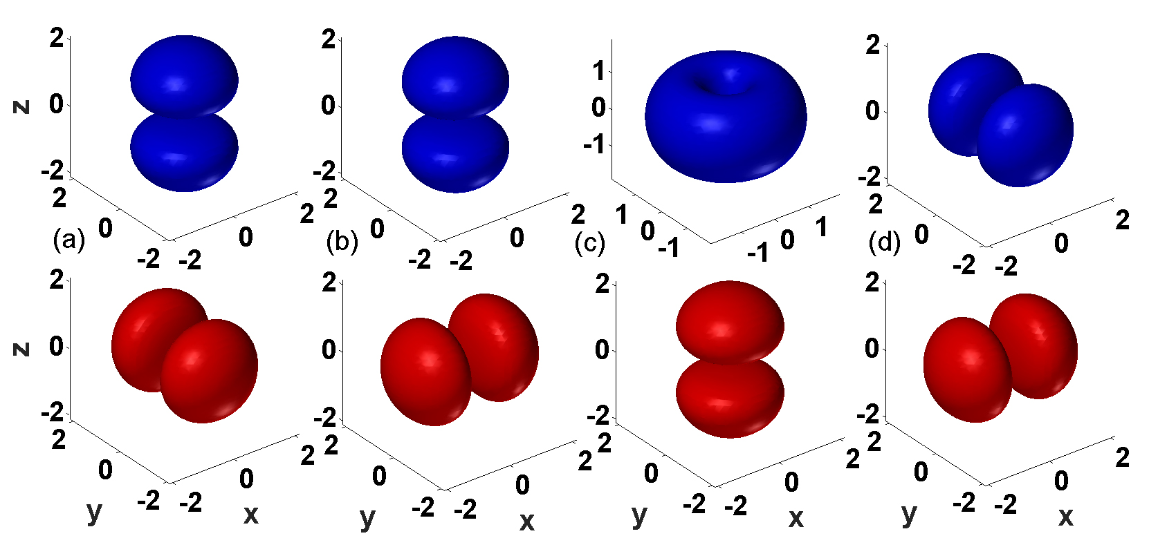
Figure 1: (Color online) Density isosurfaces, with $|\Phi|^{2}=|\Psi|^{2}=\mathrm{const}$, represent shapes of the two components (the top and bottom rows, respectively) of stationary modes that correspond to fixed points (19), (21), (23), and (27) of the Galerkin approximation, in panels (a), (b), (c), and (d), respectively. These are orthogonal dipoles with different orientations in (a), (b) and (d), and the coaxial vortex-dipole complex in (c).

The FPs found above are stationary solutions with three or two nonzero amplitudes, out of the six which constitute the GA, and a single frequency. In addition to them, a more general stationary solution of Eqs. (14), (15) can be found, with four nonvanishing amplitudes and two different frequencies:

$$a_{0}=b_{0}=0,\quad a_{\pm 1}(t)=a_{\pm}e^{-4ib^{2}t},\quad b_{\pm 1}(t)=\pm be^{-2i\left(a_{+}^{2}+a_{-}^{2}\right)t},$$ (25)

where $a_{\pm}$ and $b$ are three arbitrary real constants. There is also a mirror image of FP (25) produced by swapping $a\rightleftarrows b$. The norms (6) corresponding to FP (25) are

$$N_{a}=a_{+}^{2}+a_{-}^{2},~{}N_{b}=2b^{2}.$$ (26)

In the particular case of $a_{+}\equiv a,a_{-}=0,b=a/\sqrt{2}$, the FP (25) goes over into the above one (23), which represents the coaxial vortex-dipole complex. Another particular case corresponds to

$$a_{+}=a_{-}=b.$$ (27)

It represents to a complex built of two orthogonal dipoles oriented along the $x$ and $y$ axes, as shown in Fig. 1(d).

The investigation of the stability of FP (25) against small perturbations by means of the Bogoliubov - de Gennes equations is too cumbersome to be performed analytically. On the other hand, the energy stability can be compared to that of the above FPs, for a particular case of FP (25) with norms (26) equal to those of the solutions obtained above: $N_{a}=N_{b}=a^{2}$. For this purpose, FP (25) is taken as

$$a_{+}^{2}+a_{-}^{2}=a^{2},$$ (28)

$$a_{\pm 1}(t)=a_{\pm}e^{-2ia^{2}t}\quad b_{\pm 1}(t)=\pm\frac{a}{\sqrt{2}}e^{-2ia^{2}t},$$ (29)

which includes FP (27), as a particular case. As follows from Eqs. (12) and (13), this FP is built of a dipole in the $\Psi$ field oriented along the $z$ axis, and a mixed vortex-antivortex state in the $\Phi$ field. The calculation of the respective value of Hamiltonian (18) for the four-amplitude (4A) FP (29) yields

$$H_{\mathrm{4A}}=2a^{4}.$$ (30)

Note that expression (30) does not depend on ratio $a_{+}/a_{-}$, see Eq. (28). Thus, Eq. (30) demonstrates very broad degeneracy of the GS, in the framework of the GA: the same minimum of $H$ is realized by the FPs given by Eqs. (19), (23), and (29), including the continuous degeneracy in the 4A manifold with respect to the arbitrary value of parameter $a_{+}/a_{-}$.

Finally, simulations of the coupled GPEs (4) and (5) in imaginary time, which is a well-known numerical method for constructing stationary states of GPEs Tosi , made it easy to produce stationary solutions, which are stable in real time too, and almost exactly correspond to the FPs of the coaxial dipole-dipole and vortex-dipole types, as predicted by the FPs (19) and (23), respectively. Shapes of these solutions are very close to those displayed, in terms of Ansätze (12), (13), in the left and right columns of Fig. 1. In the regimes of moderate values of Norm where GA with the leading terms works well, the difference in measured values of Norms between the FPs predicted by GA and direct numerical stationary solutions is within few percents. On the other hand, stationary solutions close to the orthogonal-dipole mode, corresponding to FP (21), could not be obtained by means of the imaginary- (or real-) time simulations. This negative result is not surprising, as such methods cannot produce excited states whose energies exceeds the GS energy, as shown in the present case by Eq. (22).

It is relevant to mention that evident solutions with identical coaxial p-waves (vortices) in components $\Phi$ and $\Psi$, both taken as per Eq. (2), cannot be produced by the GA adopted above (because axes of the respective sets of the p-waves were chosen to be mutually orthogonal, rather than parallel). For this reason, the coaxial vortices are not considered here, but it is obvious that they are tantamount to vortex states in the single GPE with the HO trapping potential and self-repulsive nonlinearity, which were studied in detail before vortices .

Concerning the absolute GS of the model based on the coupled GPEs, with Hamiltonian (8), additional calculations (perturbative analytical and numerical) demonstrate that the obvious isotropic s-wave solution, with $l=0$, namely, $\Phi=\Psi=\exp\left(-i\mu t\right)u(r)$ (in the case of equal norms of the two components, $N_{\Phi}=N_{\Psi}$), remains the state which realizes the minimum of the energy for given norms.

IV Numerical results: Persistent time-periodic nonlinear dynamics

Numerical solutions of the coupled GPEs which generate the (energy-degenerate) GSs of the $l=1$ manifold are presented in the previous section. Here, our objective is to explore generic dynamical regimes produced by the coupled GPE system and, in parallel, by its GA counterpart.

IV.1 The interaction of obliquely oriented dipoles

As said above, pairs of mutually parallel or orthogonal dipoles, which correspond to FPs (19) or (21), respectively, form stationary states with the shapes displayed in the left and middle columns of Fig. 1 (recall that, while both these FPs are stable against small perturbations, the stationary solution of the coupled GPEs corresponding to FP (21) is difficult to find in the numerics as it corresponds to an excited state, as per Eq. (22)).

The evolution of a pair of dipoles with mutual orientation different from 0 or 90 degrees is initiated by the input

$$\Phi\left(\mathbf{r},t=0\right)=Ax\exp\left(-r^{2}/2\right),~{}\Psi\left(\mathbf{r},t=0\right)=Ax^{\prime}\exp\left(-r^{2}/2\right),$$ (31)

with amplitude $A$ and oblique angle $\theta$ between axes $x$ and $x^{\prime}$. Typical results are displayed in Fig. 2 for $\theta=40^{\circ}$ and a norm (6) of each component of $N_{\Phi}=N_{\Psi}=5.5$. Simulations of both the coupled GPEs (4), (5), and of GA equations (14), (15) reveal periodic rocking oscillations of the two dipoles, as illustrated in Fig. 2(b) by plots showing the exchange of the $y$-component of the angular momentum (the one which is different from zero in the  present case) between the two wave-function components ($\Phi$ and $\Psi$), see Eq. (7). The oscillations exhibit periodic transformations of the two components from the obliquely oriented dipoles into coaxial vortices and back, as shown in Fig. 2(a), where the periodically emerging parallel vortices (in both components) are oriented along the $y$-axis. The period of the oscillations is $T=94$ in this case.

As mentioned above, pure vortical modes with $l=1$ have the absolute value of their angular momentum equal to the norm, $M=N$. In the present case, the largest value of the angular momentum, attained in the vortex-like configurations at $t=23.6$ and $71$ in Fig. 2(a), is $\left(\left|\left(M_{y}\right)_{\Phi,\Psi}\right|\right)_{\max}~{}=2.3$, while, as said above, the norms are $N_{\Phi,\Psi}=5.5$, which implies that the periodic conversion of the wave-field configurations into the vortices is incomplete. Additional simulations demonstrate that the ratio $\left(\left|\left(M_{y}\right)_{\Phi,\Psi}\right|\right)_{\max}/N_{\Phi,\Psi}$ increases, following the growth of the norms, i.e., the conversion into the vortices is more complete for a more nonlinear system.

Finally, Fig. 2(c) clearly shows that the GA provides a rather accurate fit to the simulations of the full GPE system. In this connection, additional computations demonstrate that the share of the total norm carried by components of the full numerical solution with $l\geq 2$, which are omitted in the framework of the GA based on Eqs. (12), (13), remains $\lesssim 2\%$ in the case of $N_{\Phi}=N_{\Psi}=5.5$, thus justifying the application of the GA. Stronger nonlinearity, i.e., larger values of the total norm, gradually leads to an increase of the discrepancy of the full numerical solution from the GA (as an illustration, see Fig. 3(a) below, which shows the discrepancy in the oscillation period for a much stronger nonlinearity).

.

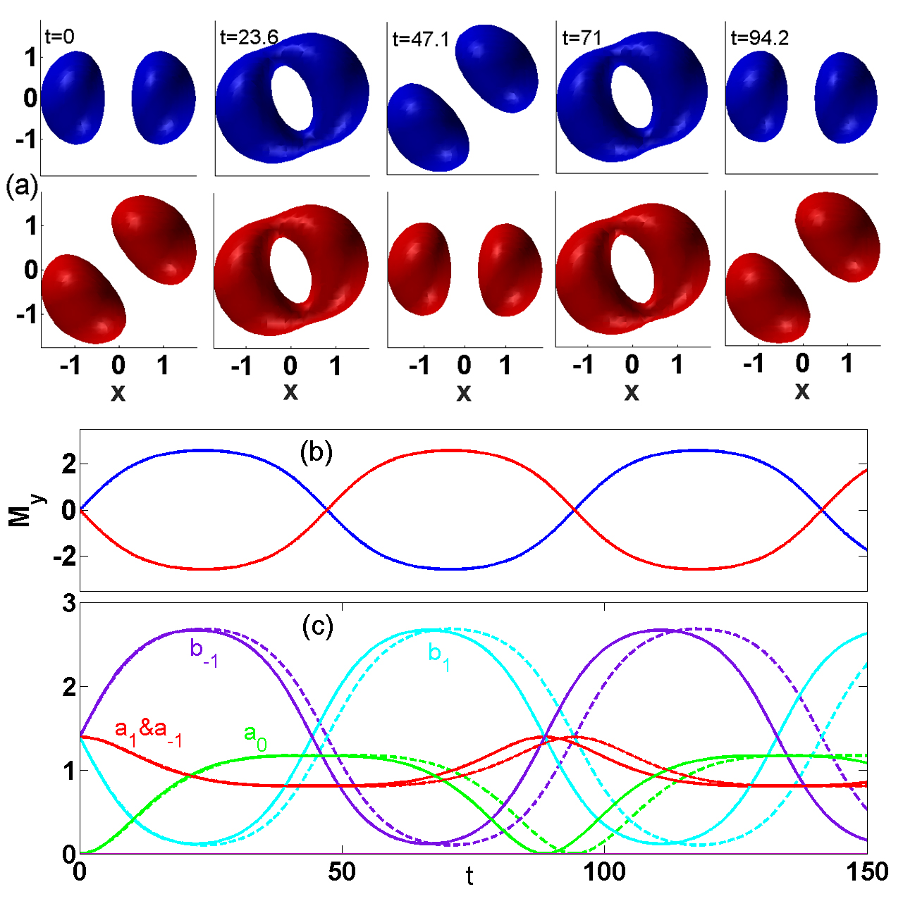
Figure 2: (Color online) Periodic oscillations of the pair of dipoles with angle $\theta=40^{\circ}$ between their orientations, initiated by input (31), with norms $N_{\Phi,\Psi}=5.5$. (a) Snapshots of the density isosurfaces of the two components, taken at moments of time indicated in the panels, within one period of the oscillations ($T\approx 94$). (b) The evolution of the $y$-component of the angular momenta of the two components, defined as per Eq. (7). (c) The evolution of the amplitudes of the GA, based on Ansätze (12), (13), as produced by simulations of Eqs. (14), (15) with initial conditions corresponding to Eq. (31) (solid curves), and the evolution of their counterparts produced by the projection of the numerically found solution of the coupled GPEs onto the Galerkin basis (dashed curves).

The dependence of the basic features of the dynamical regime on initial angle $\theta$ between the orientations of the two dipoles in the input configuration (31) is displayed in Fig. 3 for a system with stronger nonlinearity, measured by the norms, $N_{\Phi,\Psi}=22.5$, which are larger by a factor of $5$ than the case shown in Fig. 2. The results of Figs. 3(a) and (b) show a strong dependence of the oscillation period and of the efficiency of the periodic conversion of the wave-function configuration into the set of coaxial vortices, which is measured by the above-mentioned ratio $\left(\left|\left(M_{y}\right)_{\Phi,\Psi}\right|\right)_{\max}/N_{\Phi,\Psi}$, on the initial mutual-orientation angle $\theta$. It is seen that both $T$ and $\left(\left|\left(M_{y}\right)_{\Phi,\Psi}\right|\right)_{\max}/N_{\Phi,\Psi}$ attain a sharp maximum at $\theta\approx 40^{\circ}$ (the GA predicts the maximum of $T$ exactly at $\theta=45^{\circ}$, with a symmetric dependence of $T$ on $\left(\theta-45^{\circ}\right)$, in Fig. 3(a)). In fact, the difference between the full GPE dynamics and its GA-truncated version is largest precisely at $\theta=45^{\circ}$, which explains the large discrepancy in the maximum values of the GPE- and GA-predicted periods, observed in Fig. 3(a). Note also that the largest value of the momentum may even exceed the norm, viz.,$\left(\left|\left(M_{y}\right)_{\Phi,\Psi}\right|\right)_{\max}/N_{\Phi,\Psi}\approx 1.11$ at $\theta=40^{\circ}$, as can be seen in Fig. 3(b).

.

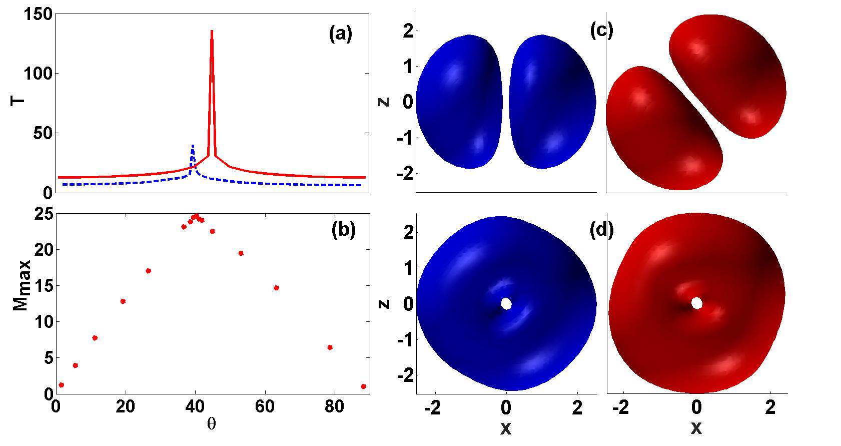
Figure 3: (Color online) Systematic results for the oscillatory dynamical regime, initiated by input (31), with initial angle $\theta$ between orientations of the two dipoles, and norms $N_{\Phi}=N_{\Psi}=22.5$ (which exceed the norms in the case shown in Fig. 2  by a factor of $5$, making the nonlinearity stronger accordingly). (a) The dependence of the oscillation period on $\theta$. The dashed blue and solid red plots display the results produced, respectively, by direct simulations of the coupled GPEs (4) and (5), and by the Galerkin approximation, i.e., by simulations of Eqs. (14), (15). (b) The largest absolute value of the angular momentum, $M_{max}\equiv\left(\left|\left(M_{y}\right)_{\Phi,\Psi}\right|\right)_{\max}$, attained in the course of the periodic evolution, versus $\theta$. (c) and (d) Snapshots of the density isosurfaces of the two wave-function components, $\left|\Phi\right|^{2}$ and $\left|\Psi\right|^{2}$, in the configurations corresponding, respectively, to the input set (at $t=0$) of two dipoles with $\theta=40^{\circ}$, and to the most complete conversion into the pair of coaxial vortices (at $t=5$), with the common axis oriented along $y$.

In this connection, it is relevant to mention that the dynamical equations of the GA (14) and (15) feature an exact scaling invariance (unlike the GPEs (4), (5), in which the scaling invariance is broken by fixing the HO length to be $1$; in that case, the precession and nutation periods are more complex functions of $1/N$, as found for cross-vortices in Ref. arxiv ). In the case of $N_{\Phi}=N_{\Psi}\equiv N/2$, this implies that the oscillation period scales as $T\sim 1/N$. Accordingly, the increase of the norm by the factor of $5$ in the case displayed in Fig. 3 for $\theta=40^{\circ}$, in comparison with the case of Fig. 2, leads to the reduction of the GA-predicted period from $T=94$ in Fig. 2 to $T\approx 19$ in Fig. 3(a).

IV.2 The interaction of mutually orthogonal dipole and vortex

The analysis of the FPs presented in the previous section has produced stable stationary solutions for the coaxial vortex-dipole complex, which corresponds to FP (23) and the right column in Fig. 1. Below we consider the dynamics initiated by an input composed of mutually perpendicular vortex in one component and dipole in the other, which are oriented in the $z$ and $y$ directions, respectively

$$\Phi\left(\mathbf{r},t=0\right)=A\left(x+iy\right)\exp\left(-r^{2}/2\right),~{}\Psi\left(\mathbf{r},t=0\right)=Ax\exp\left(-r^{2}/2\right),$$ (32)

cf. Eq. (31).

Simulations of these configurations exhibit exchange of the angular momentum between the two wave functions. Initially, the vortex donates its $z$-component of the angular momentum to the dipole, which initially carries no angular momentum. As a result, the dipole starts rotating around the $z$ axis. After a quarter of the period of the resulting oscillations (at $t=12.8$), the dipole absorbs all the angular momentum from the vortex, itself becoming a fully shaped vortex, which features the above-mentioned respective condition, $\left|M_{z}\right|=N$. Simultaneously, the original vortex component, devoid of the angular momentum, acquires a dipole-mode shape. These metamorphoses are clearly seen in the second column of snapshots displayed Fig. 4(a). At the time corresponding to a half-period, $t=25.6$, the wave functions return to their original shapes, with the dipole rotated by 90 degrees relative to its original direction (the third column in Fig. 4(a)). A nearly perfect recovery of the initial configuration in both components is observed at the end of the full period, $t=50$. Fig. 2(b) tracks the periodic exchange of the angular momentum between the two wave functions, while Fig. 2(c) demonstrates the evolution of the amplitudes of the eigenfunctions, the projection onto which corresponds to the GA. Close agreement between the GA results and their counterparts generated by simulations of the full GPE system is obtained again.

.

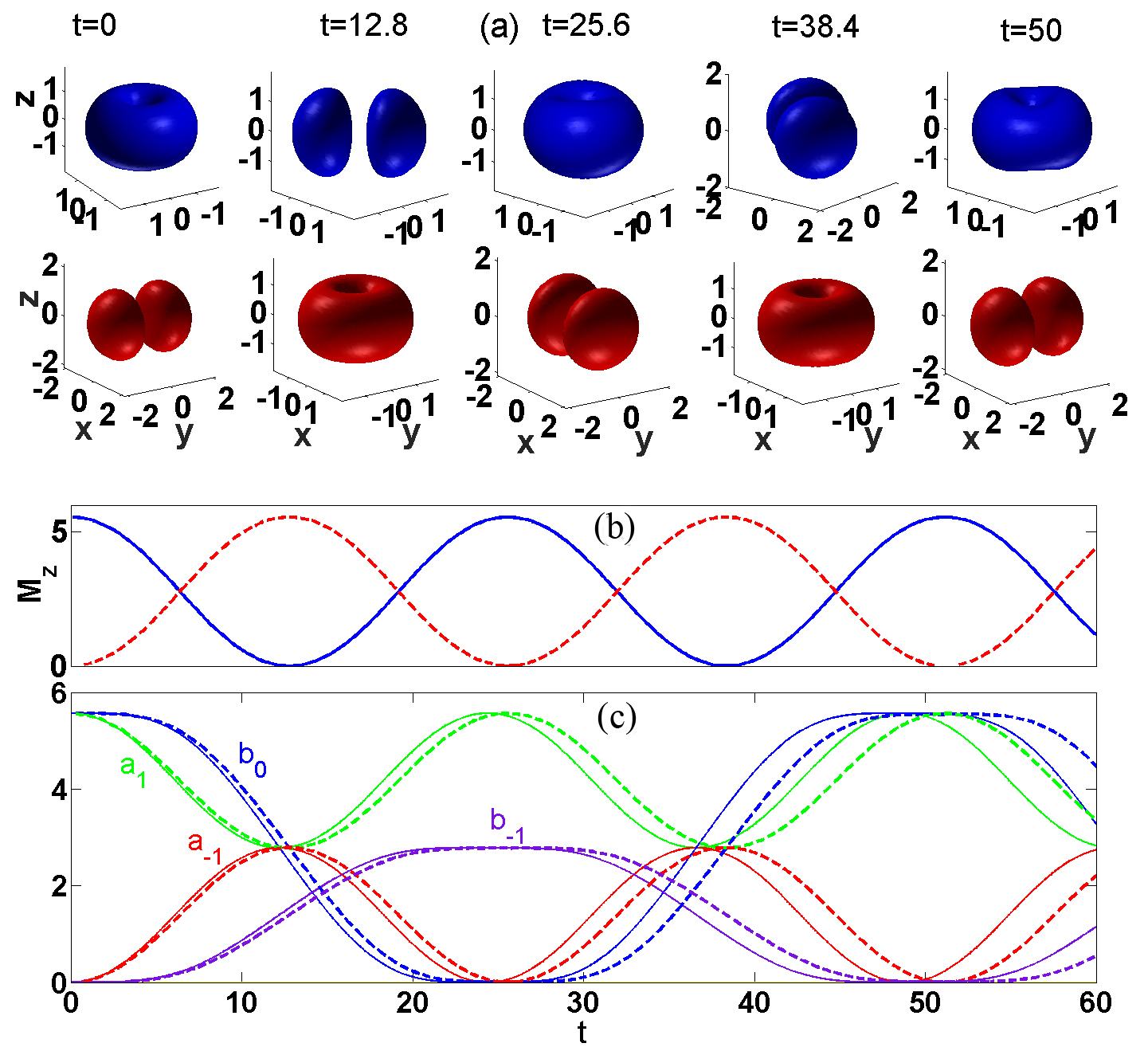
Figure 4: (Color online) (a) A set of snapshots of the density profiles of the two components illustrating the periodic evolution initiated by input (32) composed of mutually perpendicular vortex and dipole, with norms $N_{\Phi}=N_{\Psi}=5.5$. (b) The time dependence of the angular momenta, $\left(M_{z}\right)_{\Phi,\Psi}$, of the two components (blue solid and red dashed curves correspond to the components which represent the vortex and the dipole at $t=0$, respectively). (c) The evolution of the amplitudes of the eigenfunctions on which the Galerkin approximation (GA) is based. The result of simulations of the GA equations (14), (15) is shown by solid curves. Dashed curves display the results produced by the projection of the numerical solution of the full GPE system (4), (5) onto the GA modal basis.

IV.3 The interaction of non-coaxial vortices

The analysis of the FPs performed in the previous section did not produce any stationary state composed of two non-coaxial vortices. Here, we explore the dynamics initiated by a pair of identical vortices with mutually perpendicular orientations, aligned with the $z$- and $y$-axes:

$$\Phi\left(\mathbf{r},t=0\right)=A\left(x+iy\right)\exp\left(-r^{2}/2\right),~{}\Psi\left(\mathbf{r},t=0\right)=A\left(z+ix\right)\exp\left(-r^{2}/2\right),$$ (33)

fixing the amplitude as $A=1$ and norms as $N_{\Phi}=N_{\Psi}=5.56$ (this case of non-coaxial vortices was studied in arxiv , however, for a case of dominating self-phase interactions). The resulting evolution of the binary system is displayed in Fig. 5, which shows that, unlike the interacting dipoles (cf. Figs. 2 and 4), the motion does not amount to rotation about a particular axis. Instead, the vortices undergo complex deformation, related to periodic generation of all the three components of the angular momentum in each wave function, as shown in Fig. 5(c) (the net angular momentum, defined as per Eq. (7), remains conserved). The evolution of the angular momenta of each vortex is shown in vectorial (Fig. 5(b)) and scalar (Fig. 5(c)) representations. The vectorial representation (Fig. 5(b)) demonstrates the motion of the locus of each vortex axis in 3D space. The red trajectory pertains to the vortex initially aligned with the $z$-axis, while the blue trajectory corresponds to the initially $y$-oriented vortex. The trajectories features precession with nutations qualitatively similar to the case of mixed inter- and intra-species interactions reported in arxiv . Scalar representation (Fig. 5(c)) separates each component of the angular momentum and shows its evolution. Green curves solid and dashed pertain to the $z$-component of the angular momenta of each vortex respectively. Blue curves (solid and dashed) represent the evolution of the $x$-components of the angular momenta of the two vortices and finally the red curves (solid and dashed) represent the evolution of the $y$-components of the angular momenta for each of the vortices. Moreover, we present the evolution of the total angular momenta of both condensates which perfectly overlap by the violet curve. This violet curve demonstrates that in the case of the two vortices unlike the case of vortex-dipole we do not have an exchange of angular momenta between the two fields. The horizontal black line in Fig. 5(c) shows the sum of the two angular momenta which is an integral of motion. As above, Fig. 5(d) demonstrates that the GA provides an accurate description of the present dynamical regime in terms of the finite-mode truncation.

.

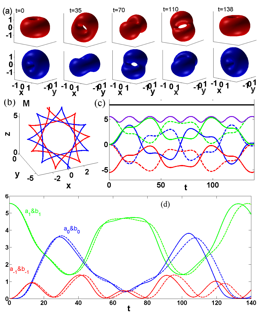
Figure 5: (Color online) The evolution of the binary system initiated by input (33) composed of two vortices, with the initial angular-momenta vectors directed along $z$ and $y$, respectively, and norms $N_{\Phi,\Psi}=5.56$. (a) Snapshots of density isosurfaces of the two components at time moments indicated in panels, within an oscillation period, $T=138$. (b) Trajectories of end points of the 3D angular-momentum vectors of the two components (the red and blue colors correspond to ones in (a)). (c) Green, red, and blue lines render, severally, the corresponding evolution of the $z$, $y$, and $x$ components of the angular momenta of the two wave function (the dashed and solid lines correspond, respectively, to the $\Phi$ and $\Psi$ wave functions). The violet curve represents the evolution of the total angular momentum of each condensate, while the horizontal black line shows the sum of the two angular momenta which remains constant. (d) The corresponding evolution of the GA amplitudes (defined by Ansätze (12) and (13)), as produced by simulations of Galerkin equations (14), (15), and by simulations of the full GPEs (4), (5), is depicted by solid and dashed lines, respectively.

Lastly, the analysis was also performed for inputs similar to the one defined by Eq. (33), but with the angle between the angular-momentum vectors of the two vortices different from $90^{\circ}$. These results (not shown) are similar to those presented here. In particular, the evolution of the two angular momenta in the vectorial form again exhibits precession-like motion combined with nutations.

V Conclusion

We have introduced a system of two 3D fields, trapped in the HO potential, which interact through the repulsive cubic nonlinearity. The system can be implemented in the form of a binary BEC, with the interaction dominated by the inter-component repulsion, that can be enhanced by means of the Feshbach resonance. Parallel to the system of two coupled GPEs (Gross-Pitaevskii equations), we have introduced a finite-mode truncation, which amounts to the six-mode GA (Galerkin approximation), based on the triplets of HO eigenstates in each component, with quantum numbers $l=1$ and $m=1,0,-1$. The first result is that FPs (fixed points) of the GA almost exactly predict the GS (ground-state) manifold for $l=1$, which features unusually broad degeneracy, including complexes in the form of a dipole coaxial with a vortex or another dipole. Dynamical regimes were initiated by inputs built as pairs of non-coaxial dipoles and/or vortices, including pairs of orthogonally oriented vortices. As a result, the system gives rise to stable dynamics, characterized by periodic conversions between dipoles and vortices. In this case too, results produced by the GA are well corroborated by direct simulations of the coupled GPEs.

As a development of the present system, it is relevant to expand it to a three-component spinor model, in which inter-component interactions may include four-wave mixing, in addition to the mutual repulsion spinor . In particular, a natural possibility will be to consider the interaction between three mutually orthogonal vortices in the three-component system trapped in a common isotropic 3D HO potential. On the other hand, the high accuracy produced by the GA in the present system suggests that this approximation may be used as an efficient tool for the study of complex stationary states and dynamical regimes in other 3D classical-field models.

- (1) M. S. Volkov and E. Wohnert, Spinning Q-balls, Phys. Rev. D 66, 085003 (2002); B. Kleihaus, J. Kunz, and Y. Shnir, Monopoles, antimonopoles, and vortex rings, ibid. 68, 101701 (2003); B. Kleihaus, J. Kunz, and Y. Shnir, Monopole-antimonopole chains and vortex rings, ibid. 70, 065010 (2004); Gravitating monopole-antimonopole chains and vortex rings, ibid. 71, 024013 (2005); J. Kunz, U. Neemann, and Y. Shnir,Transitions between vortex rings, and monopole–antimonopole chains, Phys. Lett. B 640, 57 (2006); E. Radu and M. S. Volkov, Spinning electroweak sphalerons, Phys. Rev. D 79, 065021 (2009); J. Garaud, E. Radu, and M. S. Volkov, Stable cosmic vortons, Phys. Rev. Lett. 111, 171602 (2013).
- (2) L. Faddeev and A. J. Niemi, Stable knot-like structures in classical field theory, Nature (London) 387, 58 (1997); Partially dual variables in SU(2) Yang-Mills theory, Phys. Rev. Lett. 82, 1624 (1999); E. Babaev, L. D. Faddeev, and A. J. Niemi, Hidden symmetry and knot solitons in a charged two-condensate Bose system, Phys. Rev. B 65, 100512(R) (2002); J. Jäykkä and J. M. Speight, Supercurrent coupling destabilizes knot solitons, Phys. Rev. D 84, 125035 (2011).
- (3) J. Gladikowski and M. Hellmund, Static solitons with nonzero Hopf number, Phys. Rev. D 56, 5194 (1997); H. Aratyn, L. A. Ferreira, and A. H. Zimerman, Exact static soliton solutions of (3+1)-dimensional integrable theory with nonzero Hopf numbers, Phys. Rev. Lett. 83, 723 (1999); J. Jäykkä, J. Hietarinta, and P. Salo, Topologically nontrivial configurations associated with Hopf charges investigated in the two-component Ginzburg-Landau model, Phys. Rev. B 77, 094509 (2008); J. M. Speight, Supercurrent coupling in the Faddeev–Skyrme model, J. Geom. Phys. 60, 599 (2010).
- (4) M. F. Atiyah and N. S. Manton, Phys. Lett. B 222, 438-442 (1989); C. J. Houghton, N. S. Manton, and P. M. Sutcliffe, Rational maps, monopoles and skyrmions, Nucl. Phys. B 510, 507-537 (1998).
- (5) E. Radu and M. S. Volkov, Stationary ring solitons in field theory - Knots and vortons, Phys. Rep. 468, 101 (2008).
- (6) M. Bender, P. H. Heenen, and P. G. Reinhard, Self-consistent mean-field models for nuclear structure, Rev. Mod. Phys. 75, 121 (2003); T. Sakai, and S. Sugimoto, Low energy hadron physics in holographic QCD, Prog. Theor. Phys. 113, 843-882 (2005); A. Pomarol and A. Wulzer, Baryon physics in holographic QCD, Nucl. Phys. 809, 347-361 (2009).
- (7) N. R. Cooper, Propagating magnetic vortex rings in ferromagnets, Phys. Rev. Lett. 82, 1554 (1999); S. Seki, X. Z. Yu, S. Ishiwata, and Y. Tokura, Observation of skyrmions in a multiferroic material, Science 336, 198-201 (2012); A. Fert,V. Cros, and J. Sampaio, Skyrmions on the track, Nature Nanotechnology 8, 152-156 (2013); Y. Nii, T. Nakajima, A. Kikkawa, Y. Yamasaki, K. Ohishi, J. Suzuki, Y. Taguchi, T. Arima, Y. Tokura, and Y. Iwasa, Uniaxial stress control of skyrmion phase, Nature Commun. 6, 8539 (2015); Y. Nahas, S. Prokhorenko, L. Louis, Z. Gui, I. Kornev, and L. Bellaiche, Discovery of stable skyrmionic state in ferroelectric nanocomposites, ibid. 6, 8542 (2015).
- (8) E. Babaev, Dual neutral variables and knot solitons in triplet superconductors, Phys. Rev. Lett. 88, 177002 (2002); Non-Meissner electrodynamics and knotted solitons in two-component superconductors, Phys. Rev. B 79, 104506 (2009).
- (9) A. Neubauer, C. Pfleiderer, B. Binz, A. Rosch, R. Ritz, P. G. Niklowitz, and P. Böni, Topological Hall effect in the A phase of MnSi, Phys. Rev. Lett. 102, 186602 (2009); I. Kezsmarki, S. Bordacs, P. Milde, E. Neuber, L. M. Eng, J. S. White, H. M. Ronnow, C. D. Dewhurst, M. Mochizuki, K. Yanai, H. Nakamura, D. Ehlers, V. Tsurkan, and A. Loidl, Neel-type skyrmion lattice with confined orientation in the polar magnetic semiconductor GaV4S8, Nature Materials 14, 1116 (2015).
- (10) J. Ruostekoski and J. R. Anglin, Creating vortex rings and three-dimensional skyrmions in Bose-Einstein condensates, Phys. Rev. Lett. 86, 3934 (2001); R. A. Battye, N. R. Cooper and P. M. Sutcliffe, Stable skyrmions in two-component Bose-Einstein condensates, ibid. 88, 080401 (2002); C. M. Savage and J. Ruostekoski, Energetically stable particlelike skyrmions in a trapped Bose-Einstein condensate, ibid. 91, 010403 (2003); J. Ruostekoski, and J. R. Anglin, Monopole core instability and Alice rings in spinor Bose-Einstein condensates, ibid. 91, 190402 (2003); C.-H. Hsueh, S.-C. Gou, T.-L. Horng, and Y.-M. Kao, Vortex-ring solutions of the Gross-Pitaevskii equation for an axisymmtrically trapped Bose-Einstein condensate, J. Phys. B: At. Mol. Opt. Phys. 40, 4561-4571 (2007); M. Kanász-Nagy, B. Dóra, E. A. Demler, and G. Zaránd, Stabilizing the false vacuum: Mott skyrmions. Sci. Rep. 5, 7692 (2014); T. Kaneda and H. Saito, Collision dynamics of skyrmions in a two-component Bose-Einstein condensate, Phys. Rev. A 93, 033611 (2016).
- (11) L. S. Leslie, A. Hansen, K. C. Wright, B. M. Deutsch, and N. P. Bigelow, Creation and detection of skyrmions in a Bose-Einstein condensate, Phys. Rev. Lett. 103, 250401 (2009); J. Y. Choi, W. J. Kwon, and Y. I. Shin, Observation of topologically stable 2D skyrmions in an antiferromagnetic spinor Bose-Einstein condensate, ibid. 108, 035301 (2012).
- (12) Y.-K. Liu, S. Feng, and S.-J. Yang, Stable knots in the trapped Bose-Einstein condensates, EPL 106, 50005 (2014).
- (13) Y. M. Bidasyuk, A. V. Chumachenko, O. O. Prikhodko, S. I. Vilchinskii, M. Weyrauch, and A. I. Yakimenko, Stable Hopf solitons in rotating Bose-Einstein condensates, Phys. Rev. A 92, 053603 (2015); R. N. Bisset, W. Wang, C. Ticknor, R. Carretero-González, D. J. Frantzeskakis, L. A. Collins, and P. G. Kevrekidis, Robust vortex lines, vortex rings, and hopfions in three-dimensional Bose-Einstein condensates, Phys. Rev. A 92, 063611 (2015).
- (14) M. W. Ray, E. Ruokokoski, S. Kandel, M. Möttönen, and D. S. Hall, Observation of Dirac monopoles in a synthetic magnetic field, Nature 505, 657-660 (2014); M. W. Ray, E. Ruokokoski, K. Tiurev, M. Möttönen, and D. S. Hall, Observation of isolated monopoles in a quantum field, Science 348, 544-547 (2015).
- (15) Yu. S. Kivshar and D. E. Pelinovsky, Self-Focusing and Transverse Instabilities of Solitary Waves, Phys. Rep. 331, 117 (2000); Y. S. Kivshar and G. P. Agrawal, Optical Solitons: From Fibers to Photonic Crystals (Academic Press, San Diego, 2003); B. A. Malomed, D. Mihalache, F. Wise, and L. Torner, Spatiotemporal optical solitons, J. Optics B: Quant. Semicl. Opt. 7, R53-R72 (2005); A. S. Desyatnikov, L. Torner, and Y. S. Kivshar, Optical Vortices and Vortex Solitons, Progr. Opt. 47, 1 (2005); D. Mihalache, Linear and nonlinear light bullets: recent theoretical and experimental studies, Rom. J. Phys. 57, 352-371 (2012); V. S. Bagnato, D. J. Frantzeskakis, P. G. Kevrekidis, B. A. Malomed, and D. Mihalache, Bose-Einstein condensation: Twenty years after, Rom. Rep. Phys. 67, 5-50 (2015).
- (16) Y. V. Kartashov, B. A. Malomed, and L. Torner, Solitons in nonlinear lattices, Rev. Mod. Phys. 83, 247-306 (2011).
- (17) R. McLeod, K. Wagner, and S. Blair, (3+1)-dimensional optical soliton dragging logic, Phys. Rev. A 52, 3254 (1995).
- (18) A. D. Martin and J. Ruostekoski, Quantum dynamics of atomic bright solitons under splitting and recollision, and implications for interferometry, New J. Phys. 14, 043040 (2012); J. Cuevas, P. G. Kevrekidis, B. A. Malomed, P. Dyke, and R. G. Hulet, Interactions of solitons with a Gaussian barrier: Splitting and recombination in quasi-1D and 3D, New J. Phys. 15, 063006 (2013); J. H. V. Nguyen, P. Dyke, D. Luo, B. A. Malomed, and R. G. Hulet, Collisions of matter-wave solitons, Nature Phys. 10, 918-922 (2014); G. D. McDonald, C. C. N. Kuhn, K. S. Hardman, S. Bennetts, P. J. Everitt, P. A. Altin, J. E. Debs, J. D. Close, and N. P. Robins, Bright solitonic matter-wave interferometer, Phys. Rev. Lett. 113, 013002 (2014).
- (19) L. Bergé, Wave collapse in physics: principles and applications to light and plasma waves, Phys. Rep. 303, 259-370 (1998); E. A. Kuznetsov and F. Dias, Bifurcations of solitons and their stability, Phys. Rep. 507, 43-105 (2011).
- (20) N. K. Efremidis, S. Sears, D. N. Christodoulides, J. W. Fleischer, and M. Segev, Discrete solitons in photorefractive optically induced photonic lattices, Phys. Rev. E 66, 046602 (2002); B. B. Baizakov, B. A. Malomed, and M. Salerno, Multidimensional solitons in periodic potentials, Europhys. Lett. 63, 642 (2003); J. Yang and Z. H. Musslimani, Fundamental and vortex solitons in a two-dimensional optical lattice, Opt. Lett. 28, 2094 (2003); D. Mihalache, D. Mazilu, F. Lederer, Y. V. Kartashov, L.-C. Crasovan, and L. Torner, Stable three-dimensional spatiotemporal solitons in a two-dimensional photonic lattice, Phys. Rev. E 70, 055603(R) (2004).
- (21) D. Neshev, T. J. Alexander, E. A. Ostrovskaya, Y. S. Kivshar, H. Martin, I. Makasyuk, and Z. Chen, Observation of discrete vortex solitons in optically induced photonic lattices, Phys. Rev. Lett. 92, 123903 (2004); J. W. Fleischer, G. Bartal, O. Cohen, O. Manela, M. Segev, J. Hudock, and D. N. Christodoulides, Observation of vortex-ring “discrete”solitons in 2D photonic lattices, ibid. 92, 123904 (2004).
- (22) H. Sakaguchi, B. Li, and B. A. Malomed, Creation of two-dimensional composite solitons in spin-orbit-coupled self-attractive Bose-Einstein condensates in free space, Phys. Rev. E 89, 032920 (2014).
- (23) Y.-C. Zhang, Z.-W. Zhou, B. A. Malomed, and H. Pu, Stable solitons in three dimensional free space without the ground state: Self-trapped Bose-Einstein condensates with spin-orbit coupling, Phys. Rev. Lett. 115, 253902 (2015).
- (24) L. P. Pitaevskii and S. Stringari, Bose-Einstein Condensation, Oxford University Press (Oxford, 2003).
- (25) O. V. Borovkova, Y. V. Kartashov, B. A. Malomed, and L. Torner, Algebraic bright and vortex solitons in defocusing media, Opt. Lett. 36, 3088-3090 (2011); O. V. Borovkova, Y. V. Kartashov, L. Torner, and B. A. Malomed, Bright solitons from defocusing nonlinearities, Phys. Rev. E 84, 035602 (R) (2011).
- (26) R. Driben, Y. V. Kartashov, B. A. Malomed, T. Meier, and L. Torner, Soliton gyroscopes in media with spatially growing repulsive nonlinearity, Phys. Rev. Lett. 112, 020404 (2014); Y. V. Kartashov, B. A. Malomed, Y. Shnir, and L. Torner, Twisted toroidal vortex-solitons in inhomogeneous media with repulsive nonlinearity, ibid. 113, 264101 (2014); R. Driben, Y. Kartashov, B. A. Malomed, T. Meier, and L. Torner, Three-dimensional hybrid vortex solitons, New J. Phys. 16, 063035 (2014); R. Driben, N. Dror, B. Malomed, and T. Meier, Multipoles and vortex multiplets in multidimensional media with inhomogeneous defocusing nonlinearity, ibid. 17, 083043 (2015); R. Driben, T. Meier, and B. A. Malomed, Creation of vortices by torque in multidimensional media with inhomogeneous defocusing nonlinearity, Sci. Rep. 5, 9420 (2015).
- (27) S. Sinha, Semiclassical analysis of collective excitations in Bose-Einstein condensate, Phys. Rev. A 55, 4325 (1997); R. J. Dodd, K. Burnett, M. Edwards, and C. W. Clark, Excitation spectroscopy of vortex states in dilute Bose-Einstein condensed gases, ibid. 56, 587 (1997); T. Isoshima, M. Nakahara, T. Ohmi, and K. Machida, Creation of a persistent current and vortex in a Bose-Einstein condensate of alkali-metal atoms, ibid. 61, 063610 (2000); A. A. Svidzinsky and A. L. Fetter, Stability of a vortex in a trapped Bose-Einstein condensate, Phys. Rev. Lett. 84, 5919 (2000); V. M. Lashkin, Stable three-dimensional spatially modulated vortex solitons in Bose-Einstein condensates, Phys. Rev. A 78, 033603 (2008); T. P. Simula, T. Mizushima, and K. Machida, Vortex waves in trapped Bose-Einstein condensates, ibid. 78, 053604 (2008).
- (28) L. C. Crasovan, G. Molina-Terriza, J. P. Torres, L. Torner, V. M. Pérez-García, and D. Mihalache, Globally linked vortex clusters in trapped wave fields, Phys. Rev. E 66, 036612 (2002); L. C. Crasovan, V. Vekslerchik, V. M. Pérez-García, J. P. Torres, D. Mihalache, and L. Torner, Stable vortex dipoles in nonrotating Bose-Einstein condensates. Phys. Rev. A 68, 063609 (2003); V. M. Lashkin, Two-dimensional multisolitons and azimuthons in Bose-Einstein condensates, ibid. 77, 025602 (2008); S. Middelkamp, P. J. Torres, P. G. Kevrekidis, D. J. Frantzeskakis, R. Carretero-González, P. Schmelcher, D. V. Freilich, and D. S. Hall, Guiding-center dynamics of vortex dipoles in Bose-Einstein condensates, ibid. 84, 011605 (R) (2011).
- (29) G. A. Swartzlander, Jr. and C. T. Law, Optical vortex solitons observed in Kerr nonlinear media, Phys. Rev. Lett. 69, 2503 (1992); M. R. Matthews, B. P. Anderson, P. C. Haljan, D. S. Hall, C. E. Wieman, and E. A. Cornell, Vortices in a Bose-Einstein condensate, Phys. Rev. Lett. 83, 2498 (1999); B. P. Anderson, P. C. Haljan, C. A. Regal, D. L. Feder, L. A. Collins, C. W. Clark, and E. A. Cornell, Watching dark solitons decay into vortex rings in a Bose-Einstein condensate, ibid. 86, 2926 (2001); A. E. Leanhardt, A. Görlitz, A. P. Chikkatur, D. Kielpinski, Y. I. Shin, D. E. Pritchard, and W. Ketterle, Imprinting vortices in a Bose-Einstein condensate using topological phases, ibid. 89, 190403 (2002); V. Bretin, P. Rosenbusch, F. Chevy, G. V. Shlyapnikov, and J. Dalibard, Quadrupole oscillation of a single-vortex Bose-Einstein condensate: Evidence for Kelvin modes, ibid. 90, 100403 (2003).
- (30) A. L. Fetter, Rotating trapped Bose-Einstein condensates, Rev. Mod. Phys. 81, 647 (2009).
- (31) J. J. García-Ripoll and V. M. Pérez-García, Stable and unstable vortices in multicomponent Bose-Einstein condensates, Phys. Rev. Lett. 84, 4264 (2000); K. Kasamatsu, M. Tsubota, and M. Ueda, Vortices in multicomponent Bose-Einstein condensates, Int. J. Mod. Phys. B 19, 1835-1904 (2005); K. M. Mertes, J. W. Merrill, R. Carretero-González, D. J. Frantzeskakis, P. G. Kevrekidis, and D. S. Hall, Nonequilibrium dynamics and superfluid ring excitations in binary Bose-Einstein condensates, Phys. Rev. Lett. 99, 190402 (2007); R. Zamora-Zamora, M. Lozada-Hidalgo, S. F. Caballero-Benítez, and V. Romero-Rochín, Vortices on demand in multicomponent Bose-Einstein condensates, Phys. Rev. A 86, 053624 2012).
- (32) R. Driben, V. V. Konotop, and T. Meier, Precession and nutation dynamics of nonlinearly coupled non-coaxial three-dimensional matter wave vortices, Sci. Rep. 6, 22758 (2016).
- (33) S. Brenner and R. L. Scott, The Mathematical Theory of Finite Element Methods, Springer-Verlag (New York, 2002); J. L. Guermond, P. Minev, and J. Shen, An overview of projection methods for incompressible flows, Comp. Methods Appl. Mech. Engineering 195, 6011-6045 (2006).
- (34) A. M. Kaufman, R. P. Anderson, T. M. Hanna, E. Tiesinga, P. S. Julienne, and D. S. Hall, Radio-frequency dressing of multiple Feshbach resonance, Phys. Rev. A 80, 050701(R) (2009).
- (35) S. Tojo, Y. Taguchi, Y. Masuyama, T. Hayashi, H. Saito, and T. Hirano, Controlling phase separation of binary Bose-Einstein condensates via mixed-spin-channel Feshbach resonance, Phys. Rev. A 82, 033609 (2010).
- (36) D. J. Papoular, G. V. Shlyapnikov, and J. Dalibard, Microwave-induced Fano-Feshbach resonances, Phys. Rev. A 81, 041603(R) (2010); T. V. Tscherbul, T. Calarco, I. Lesanovsky, R. V. Krems, A. Dalgarno, and J. Schmiedmayer, rf-field-induced Feshbach resonances, Phys. Rev. A 81, 050701(R) (2010).
- (37) M. Egorov, B. Opanchuk, P. Drummond, B. V. Hall, P. Hannaford, and A. I. Sidorov, Measurement of s-wave scattering lengths in a two-component Bose-Einstein condensate, Phys. Rev. A 87, 053614 (2013).
- (38) B. D. Esry, C. H. Greene, J. P. Burke, Jr., and J. L. Bohn, Hartree-Fock theory for double condensates, Phys. Rev. Lett. 78, 3594-3597 (1997); M. L. Chiofalo, S. Succi, and M. P. Tosi, Ground state of trapped interacting Bose-Einstein condensates by an explicit imaginary-time algorithm. Phys. Rev. E 62, 7438-7444 (2000); W. Bao and Q. Du, Computing the ground state solution of Bose-Einstein condensates by a normalized gradient flow, SIAM J. Sci. Comput. 25, 1674-1697 (2004).
- (39) T. Isoshima, M. Nakahara, T. Ohmi, and K. Machida, Creation of a persistent current and vortex in a Bose-Einstein condensate of alkali-metal atoms, Phys. Rev. A 61, 063610 (2000); Y. Kawaguchi and M. Ueda, Spinor Bose-Einstein condensates, Phys. Rep. 520, 253-381 (2012).