The Herschel Orion Protostar Survey: Spectral Energy Distributions and Fits Using a Grid of Protostellar Models

Abstract

We present key results from the Herschel Orion Protostar Survey (HOPS): spectral energy distributions (SEDs) and model fits of 330 young stellar objects, predominantly protostars, in the Orion molecular clouds. This is the largest sample of protostars studied in a single, nearby star formation complex. With near-infrared photometry from 2MASS, mid- and far-infrared data from Spitzer and Herschel, and submillimeter photometry from APEX, our SEDs cover 1.2 – 870 $\mu$m and sample the peak of the protostellar envelope emission at $\sim$ 100 $\mu$m. Using mid-IR spectral indices and bolometric temperatures, we classify our sample into 92 Class 0 protostars, 125 Class I protostars, 102 flat-spectrum sources, and 11 Class II pre-main-sequence stars. We implement a simple protostellar model (including a disk in an infalling envelope with outflow cavities) to generate a grid of 30,400 model SEDs and use it to determine the best-fit model parameters for each protostar. We argue that far-IR data are essential for accurate constraints on protostellar envelope properties. We find that most protostars, and in particular the flat-spectrum sources, are well fit. The median envelope density and median inclination angle decrease from Class 0 to Class I to flat-spectrum protostars, despite the broad range in best-fit parameters in each of the three categories. We also discuss degeneracies in our model parameters. Our results confirm that the different protostellar classes generally correspond to an evolutionary sequence with a decreasing envelope infall rate, but the inclination angle also plays a role in the appearance, and thus interpretation, of the SEDs.

ApJS, in press

1 Introduction

The formation process of low- to intermediate-mass stars is divided into several stages, ranging from the deeply embedded protostellar stage to the period when a young star is dispersing its protoplanetary disk in which planets may have formed. During the protostellar phase, which is estimated to last $\sim$ 0.5 Myr (Evans et al., 2009; Dunham et al., 2014), the growing central source accretes dust and gas from a collapsing envelope. The material from the envelope is most likely accreted through a disk, feeding the growing star. A fraction of the mass is ejected in outflows, which carve openings into the envelope along the outflow axis. Despite our understanding of the basic processes operating in low-mass protostars, fundamental questions remain (e.g., Dunham et al., 2014). In particular, it is not understood how the processes of infall, feedback from outflows, disk accretion, as well as the surrounding birth environment, affect mass accretion and determine the ultimate stellar mass. The luminosity of protostars, which can be dominated by accretion, is observed to span more than three orders of magnitude, yet the underlying physics of this luminosity range is also not understood (Dunham et al., 2010; Offner & McKee, 2011). It is in this protostellar phase that disks are formed, setting the stage for planet formation, yet how infall, feedback, accretion, and environment influence the properties of disks and of planets that eventually form from them is unknown. The large samples of well-characterized protostars identified from surveys with Spitzer and Herschel now provide the means to systematically study the processes controlling the formation of stars and disks; the goal of this work is to provide such a characterization for the protostars found in the Orion A and B clouds, the largest population of protostars for any of the molecular clouds within 500 pc of the Sun (Kryukova et al., 2012; Dunham et al., 2013, 2015).

In protostars, dust in the disk and envelope reprocesses the shorter-wavelength radiation emitted by the central protostar and the accretion shock on the stellar surface and reemits it prominently at mid- to far-infrared wavelengths. As a result, the combined emission of most protostellar systems (consisting of protostar, disk, and envelope) peaks in the far-IR. Young, deeply embedded protostars have spectral energy distributions (SEDs) with steeply rising slopes in the infrared, peaking around 100 µm, and large fractional submillimeter luminosities (e.g., Enoch et al., 2009; Stutz et al., 2013). Near 10 µm and 18 µm, absorption by sub-micron-sized silicate grains causes broad absorption features; in addition, there are several ice absorption features across the infrared spectral range (Boogert et al., 2008; Pontoppidan et al., 2008). These absorption features are indicative of the amount of material along the line of sight, with the deepest features found for the most embedded objects. In addition, due to the asymmetric radiation field, the orientation of a protostellar system to the line of sight, whether through a dense disk or a low-density cavity, plays a role in the appearance of the SED. It influences the near- to far-IR slope, the depth of the silicate feature, the emission peak, and the fraction of light emitted at the longest wavelengths (see, e.g., Whitney et al., 2003a).

To classify young stellar objects (YSOs) into observational classes, the near- to mid-infrared spectral index $n$ ($\lambda F_{\lambda}\propto\lambda^{n}$) from about 2 to 20 $\mu$m has traditionally been used (Lada, 1987; Adams, Lada, & Shu, 1987; André & Montmerle, 1994; Evans et al., 2009; Dunham et al., 2014). This index is positive for a Class 0/I protostar, between $-0.3$ and 0.3 for a flat-spectrum source, and between $-1.6$ and $-0.3$ for a Class II pre-main-sequence star. Class 0 protostars are distinguished from Class I protostars as having $L_{submm}/L_{bol}$ ratios larger than 0.5%, according to the original definition by André et al. (1993). Other values for this threshold that have recently been used are 1% (Sadavoy et al., 2014) and even 3% (Maury et al., 2011). Another measure for the evolution of a young star is the bolometric temperature ($T_{bol}$), which is the temperature of a blackbody with the same flux-weighted mean frequency as the observed SED (Myers & Ladd, 1993). A Class 0 protostar has $T_{bol}<70$ K, a Class I protostar 70 K $<T_{bol}<$ 650 K, and a Class II pre-main-sequence star 650 K $<T_{bol}<$ 2800 K (Chen et al., 1995). These observational classes are inferred to reflect evolutionary stages, with the inclination angle to the line of sight being the major source of uncertainty in translating classes to “stages” (Robitaille et al., 2006; Evans et al., 2009). Also the accretion history, which likely includes episodic accretion events and thus temporary increases in luminosity, adds to this uncertainty (Dunham et al., 2010; Dunham & Vorobyov, 2012). Protostars with infalling envelopes of gas and dust correspond to Stages 0 and I, with the transition from Stage 0 to I occurring when the stellar mass becomes larger than the envelope mass (Dunham et al., 2014). Young stars that have dispersed their envelopes and are surrounded by circumstellar disks correspond to Stage II.

By modeling the SEDs of protostars, properties of their envelopes, and to some extent of their disks, can be constrained. The near-IR is particularly sensitive to extinction and thus constrains the inclination angle and cavity opening angle, as well as the envelope density. Mid-IR spectroscopy reveals the detailed emission around the silicate absorption feature and thus provides additional constraints for both disk and envelope properties (see, e.g., Furlan et al., 2008). At longer wavelengths, envelope emission starts to dominate. Thus, photometry in the far-IR is necessary to determine the peak of the SED and constrain the total luminosity and envelope properties.

Here we present 1.2–870 $\mu$m SEDs and radiative transfer model fits of 330 YSOs, most of them protostars, in the Orion star formation complex. This is the largest sample of protostars studied in a single, nearby star-forming region (distance of 420 pc; Menten et al. 2007; Kim et al. 2008) and therefore significant for advancing our understanding of protostellar structure and evolution. These protostars were identified in Spitzer Space Telescope (Werner et al., 2004) data by Megeath et al. (2012) and were observed at 70 and 160 µm with the Photodetector Array Camera and Spectrometer (PACS; Poglitsch et al., 2010) on the Herschel Space Observatory (Pilbratt et al., 2010) as part of the Herschel Orion Protostar Survey (HOPS), a Herschel open-time key program (e.g., Fischer et al., 2010; Stanke et al., 2010; Manoj et al., 2013; Stutz et al., 2013, W. J. Fischer et al. 2016, in preparation; B. Ali et al. 2016, in preparation). To extend the SEDs into the sub-mm, most of the YSOs were also observed in the continuum at 350 and 870 $\mu$m with the Atacama Pathfinder Experiment (APEX) telescope (Stutz et al., 2013). Our sample also includes 16 new protostars identified in PACS data obtained by the HOPS program (Stutz et al. 2013; Tobin et al. 2015; see section 2). We use a grid of 30,400 protostellar model SEDs to find the best fit to the SED for each object and constrain its protostellar properties. As mentioned above, the far-infrared data add crucial constraints for the model fits, given that for most protostars the SED peaks in this wavelength region, and therefore, within the framework of the model grid, our SED fits yield the most reliable protostellar parameters to date for these sources.

2 Sample Description

The 488 protostars identified in Spitzer data by Megeath et al. (2012) represent the basis for the HOPS sample (see Fischer et al., 2013; Manoj et al., 2013; Stutz et al., 2013). They have 3.6-24 $\mu$m spectral indices $\geq$ $-0.3$ and thus encompass flat-spectrum sources. To be included in the target list for the PACS observations, the predicted flux of a protostar in the 70 $\mu$m PACS band had to be at least 42 mJy as extrapolated from the Spitzer SED. Since targets were required to have a 24 $\mu$m detection, protostars in the Orion Nebula – where the Spitzer 24 $\mu$m data are saturated – are excluded. In addition, after the PACS data were obtained, several new point sources that were very faint or undetected in the Spitzer bands were discovered in the Herschel data (Stutz et al., 2013). Fifteen of them were found to be reliable new protostars. One more protostar, which was not included in the sample of Stutz et al. (2013) due to its more spatially extended appearance at 70 $\mu$m, was recently confirmed by Tobin et al. (2015). We have added these 16 protostars to the HOPS sample for this work (see Table D1 in the Appendix). Most of these new protostars have very red colors and are thus potentially the youngest protostars identified in Orion (see Stutz et al., 2013).

Each object in the target list was assigned a “HOPS” identification number, resulting in 410 objects with such numbers; HOPS 394 to 408 are the new protostars identified by Stutz et al. (2013), and HOPS 409 is the new protostar from Tobin et al. (2015). Four of the 410 HOPS targets turned out to be duplicates, and 31 are likely extragalactic contaminants (see Appendix D.2.2 for details). Some objects in the HOPS target list were not observed by PACS; of these 33 objects, 16 are likely contaminants, while the remaining objects were originally proposed but were not observed since they were too faint to have been detected with PACS in the awarded observing time. In addition, 35 HOPS targets were not detected at 70 µm (see Appendices D.2.1 and D.2.2); eight of these are considered extragalactic contaminants, while two of them (HOPS 349 and 381) have only two measured flux values each, making their nature more uncertain. One more target, HOPS 350, also has just two measured flux values (at 24 and 70 $\mu$m) and is therefore also excluded from the analysis of this paper. Similarly, we excluded HOPS 352, since it was only tentatively detected at 24 µm (it lies on the Airy ring of HOPS 84) and in none of the other data sets.

To summarize, starting from the sample of 410 HOPS targets, but excluding likely contaminants and objects not observed or detected by PACS, there are 330 remaining objects that have Spitzer and Herschel data and are considered protostars (based on their Spitzer classification from Megeath et al. 2012). They form the sample studied in this work. Their SEDs are presented in the next section, and in later sections we show and discuss the results of SED fits for these targets. Their coordinates, SED properties, and classification, as well as their best-fit model parameter values, are listed in Table A1. The 41 likely protostars that lack PACS data (either not observed or not detected) are presented in Appendix D.2.1.

3 Spectral Energy Distributions

3.1 Data

Table 1: SED Data for the HOPS targets

Object	$J$ Flux	$J$ Unc.	$J$ Flag	$\cdots$	[70] Flux	[70] Unc.	[70] Flag	$\cdots$	[870] Flux	[870] Unc.	[870] Flag	Object	[5.4] Flux	[5.4] Unc.	$\cdots$	[35] Flux	[35] Unc.	IRS scaling
HOPS 1	0.000E+00	0.000E+00	3	$\cdots$	3.697E+00	1.850E-01	1	$\cdots$	6.354E-01	1.271E-01	2		8.631E-03	6.069E-04	$\cdots$	1.185E+00	6.460E-02	1.17
HOPS 2	2.770E-04	5.000E-05	1	$\cdots$	5.188E-01	2.617E-02	1	$\cdots$	3.865E-01	7.730E-02	2		4.360E-02	3.757E-03	$\cdots$	3.704E-01	3.035E-02	1.00
HOPS 3	2.198E-03	8.900E-05	1	$\cdots$	3.187E-01	1.622E-02	1	$\cdots$	1.201E-01	2.402E-02	1		4.460E-02	7.925E-03	$\cdots$	4.050E-01	2.443E-02	1.66
HOPS 4	3.820E-04	5.300E-05	1	$\cdots$	6.116E-01	3.083E-02	1	$\cdots$	1.840E-01	3.680E-02	2		2.055E-02	1.240E-03	$\cdots$	4.943E-01	3.484E-02	1.00
HOPS 5	0.000E+00	0.000E+00	3	$\cdots$	7.103E-01	3.573E-02	1	$\cdots$	6.973E-02	1.395E-02	2		1.475E-02	2.695E-03	$\cdots$	3.077E-01	4.484E-03	1.00
HOPS 6	0.000E+00	0.000E+00	3	$\cdots$	9.110E-02	5.523E-03	1	$\cdots$	2.311E-01	4.622E-02	2		1.271E-03	3.935E-04	$\cdots$	5.350E-02	5.244E-03	1.00
HOPS 7	0.000E+00	0.000E+00	3	$\cdots$	1.342E+00	6.728E-02	1	$\cdots$	3.577E-01	7.154E-02	2		6.459E-04	3.090E-04	$\cdots$	3.258E-01	2.114E-02	1.00

Note. — Each object has up to 13 photometric data points and 16 IRS data points (see Section 5). Here we only show some of the data points for a few HOPS targets. For each measurement, we provide the measured flux in Jy, its uncertainty (also in Jy) and, for the photometry only, a flag value (0—not observed, 1—measured, 2—upper limit, 3—not detected). For those HOPS targets with IRS spectra, we also provide the scaling factor that was applied to all IRS fluxes in each spectrum to bring them in agreement with the IRAC and MIPS fluxes (see Section 5 for details).

To convert the 2MASS magnitudes and the Spizter magnitudes from Megeath et al. (2012) to fluxes, we used the following zero points: 1594 Jy for $J$, 1024 Jy for $H$, 666.7 Jy for $K_{s}$, 280.9 Jy for [3.6], 179.7 Jy for [4.5], 115.0 Jy for [5.8], 64.1 Jy for [8], and 7.17 Jy for [24] (2MASS: Cohen et al. 2003; IRAC: Reach et al. 2005; MIPS: Engelbracht et al. 2007).

This table is published in its entirety in the machine-readable format on the journal website. A portion is shown here for guidance regarding its form and content.

In order to construct SEDs for our sample of 330 YSOs, we combined our own observations with data from the literature and existing catalogs. For the near-infrared photometry, we used $J$, $H$, and $K_{s}$ data from the Two Micron All Sky Survey (2MASS; Skrutskie et al., 2006). For the mid-infrared spectral region, we used Spitzer data from Kryukova et al. (2012) and Megeath et al. (2012): the Infrared Array Camera (IRAC; Fazio et al., 2004) provided 3.6, 4.5, 5.8, and 8.0 µm photometry, while the Multiband Imaging Photometer for Spitzer (MIPS; Rieke et al., 2004) provided 24 µm photometry. In addition, most of the YSOs in the HOPS sample were also observed with the Infrared Spectrograph (IRS; Houck et al., 2004) on Spitzer using the Short-Low (SL; 5.2-14 µm) and Long-Low (LL; 14-38 µm) modules, both with a spectral resolution of about 90 (see, e.g., Kim et al. (2016) for a description of IRS data reduction). Herschel PACS data at 70, 100, and 160 µm yielded far-infrared photometric data points (B. Ali et al. 2016, in preparation; the 100 $\mu$m data are from the Gould Belt Survey; e.g., André et al. 2010). Most YSOs were also observed at 350 and 870 µm (see Stutz et al. 2013) by the APEX telescope using the SABOCA and LABOCA instruments (Siringo et al., 2010, 2009, respectively). Thus, our SEDs have well-sampled wavelength coverage from 1.2 to 870 $\mu$m; we did not include additional data from the literature in order to preserve a homogeneous data set for all the objects in our sample.

The aperture radius used for the photometry varies depending on the instrument and wave band. The photometry in the 2MASS catalog was derived from point-spread function (PSF) fits using data from 4″ apertures around each object (see the Explanatory Supplement to the 2MASS All Sky Data Release and Extended Mission Products). Megeath et al. (2012) used an aperture radius of 2$\farcs$4 for IRAC and PSF photometry for MIPS 24 $\mu$m data. We used aperture radii of 9$\farcs$6 and sky annuli of 9$\farcs$6-19$\farcs$2 for PACS 70 and 100 µm images; we then applied aperture correction factors of 0.7331 and 0.6944 to the 70 and 100 µm fluxes, respectively. For PACS 160 µm, we used an aperture radius of 12$\farcs$8, a sky annulus of 12$\farcs$8-25$\farcs$6, and an aperture correction factor of 0.6602. In some cases (background contamination, close companions) we used PSF photometry at 70 and 160 $\mu$m instead (see B. Ali et al. 2016, in preparation, for details). Finally, we adopted beam fluxes at 350 and 870 $\mu$m (with FWHMs of 7$\farcs$34 and 19″, respectively). The IRS SL module has a slit width of 3$\farcs$6, while the LL module is wider, with a slit width of 10$\farcs$5. Sometimes the flux level of the two segments did not match at 14 $\mu$m (due to slight mispointings or more extended emission from surrounding material measured in LL), and in these cases usually the SL spectrum was scaled by at most a factor of $\sim$ 1.4 (typically 1.1-1.2). In a few cases, especially when the LL spectrum included substantial amounts of extended emission or flux from a nearby object, the LL spectrum was scaled down to match the flux level of the SL spectrum at 14 $\mu$m, typically by a factor of 0.8-0.9. We discuss how the different aperture sizes are accounted for in the model fluxes in section 4.2.

The SEDs of our HOPS sample are shown in Figure A53 together with their best-fit models from our model grid (see sections below); the data are listed in Table 1. Many objects display a deep silicate absorption feature at 10 $\mu$m and ice features in the 5-8 $\mu$m region, as expected for protostars. Those objects with very deep 10 $\mu$m features and steeply rising SEDs are likely deeply embedded protostars, often seen at high inclination angles.

3.2 Multiplicity and Variability

A large fraction (203 out of 330) of the young stars in our sample have at least one Spitzer-detected source within a radius of 15″; in most cases, this “companion” is faint in the infrared and likely a background star or galaxy. Thus, the emission at far-IR and sub-mm wavelengths is expected to be dominated by the protostar or pre-main-sequence star, and we can assume that the SEDs are representative of the YSOs even if the nearby sources cannot be separated at these wavelengths. There are a few YSOs that have objects separated by just 1″-3″ and are only resolved in one or two IRAC bands (HOPS 22, 78, 108, 184, 203, 247, 293, 364); in these cases we used the flux at the IRAC position that most closely matched those at longer wavelengths. We note that some of these very close “companions” are likely outflow knots. There are also unresolved binaries, which appear as single sources even in the IRAC observations (Kounkel et al., 2016); in these cases our SEDs show the combined flux in all wave bands. If two point sources are not fully resolved and the resulting blended source is elongated, no IRAC photometry was extracted. In such cases, a protostar may not have IRAC fluxes even though it was detected in the Spitzer images.

There are also several protostars that lie close to other protostars: HOPS 66 and 370 ($d$=14.9″), HOPS 76 and 78 ($d$=14.1″), HOPS 86 and 87 ($d$=12.1″), HOPS 117 and 118 ($d$=13.7″), HOPS 121 and 123 ($d$=7.6″), HOPS 124 and 125 ($d$=9.8″), HOPS 165 and 203 ($d$=13.3″), HOPS 175 and 176 ($d$=8.0″), HOPS 181 and 182 ($d$=10.2″), HOPS 225 and 226 ($d$=9.2″), HOPS 239 and 241 ($d$=12.4″), HOPS 262 and 263 ($d$=6.3″), HOPS 316 and 358 ($d$=6.9″), HOPS 332 and 390 ($d$=11.2″), HOPS 340 and 341 ($d$=4.7″), and HOPS 386 and 387 ($d$=9.9″). HOPS 105 lies 8.7″ to the north of an infrared-bright source, identified by Megeath et al. (2012) as a young star with a protoplanetary disk. This source is brighter than HOPS 105 in all Spitzer bands and at 70 $\mu$m, but it is well separated at all wavelengths. A similar situation applies to HOPS 128, which has a disk-dominated source 6.3″ to the southeast. HOPS 108 is 6.6″ from HOPS 64, which is brighter than HOPS 108 out to 8 $\mu$m, but not detected in the far-IR and sub-mm. HOPS 108 also lies 16.6″ from HOPS 369 and 28.2″ from HOPS 370. HOPS 140 has two neighboring sources, at 9.6″ and 13.9″, that are likely surrounded by protoplanetary disks; they are both brighter than HOPS 140 out to 8 $\mu$m, but at 70 $\mu$m and beyond HOPS 140 dominates. HOPS 144 lies 7.9″ from HOPS 377; there is also a somewhat fainter, red source 11.7″ to the northeast, which is not detected beyond 24 $\mu$m. This source also lies 9.7″ to the southwest of HOPS 143. HOPS 173 forms a small cluster with HOPS 174 (at 7.1″) and HOPS 380 (at 11.4″); HOPS 174 is the brightest source out to 24 $\mu$m, but at 70 $\mu$m HOPS 173 takes on this role. Also HOPS 322, 323, and 389 form a group of protostars; HOPS 322 lies 13.4″ from HOPS 389 and 20.1″ from HOPS 323, while HOPS 323 and 389 are 10.2″ apart. HOPS 323 is the brightest source.

Thus, there are 45 targets in our sample that have an object within 15″ that is bright in the mid- or far-IR and that is resolved with IRAC and MIPS. Given that Megeath et al. (2012) used PSF photometry for the MIPS 24 $\mu$m observations, they obtained reliable fluxes even for companions separated by less than 6″, the typical PSF FWHM. For fluxes at 70 and 160 $\mu$m, we also used PSF photometry for objects that were point sources, but too close for aperture photometry. In cases where the fluxes could not be determined even with PSF photometry, we had to adopt upper limits instead. Similarly, we performed PSF photometry on protostars without companions, but contaminated by extended or filamentary emission; if the PSF photometry did not return a good fit, we used the flux value from aperture photometry as an upper limit.

Since most of our targets have an IRS spectrum, in addition to data points from IRAC at 5.8 and 8 µm and from MIPS at 24 µm, we can detect discrepancies if flux values at similar wavelengths, but from different instruments, do not agree. They might be due to calibration or extraction problems in the IRS spectrum (for example, some extended emission around the target or a close companion), but also to variability. We assumed the former scenario if the flux deviations between IRS and IRAC and between IRS and MIPS were similar (and more than 10%, a conservative estimate for the typical calibration uncertainty), and in such cases scaled the IRS spectrum to the MIPS 24 µm flux. Even though this scaling could mask actual variability, it creates a representative SED for the YSO and yields an estimate of the protostellar parameters from model fits of the SED.

Figure 1: Histograms of the 4.5-24 $\mu$m spectral indices (left), bolometric temperatures (middle), and bolometric luminosities (right) for the 330 YSOs in our sample.

In Appendix B we identify potentially variable HOPS targets based on their mid-IR fluxes and find that about 5% of the protostars with IRS, IRAC, and MIPS data could be variable. The Young Stellar Object Variability (YSOVAR) program, which monitored large samples of protostars and pre-main-sequence stars in nearby star-forming regions with Spitzer at 3.6 and 4.5 $\mu$m (Morales-Calderón et al., 2011; Cody et al., 2014; Rebull et al., 2014; Günther et al., 2014; Poppenhaeger et al., 2015; Wolk et al., 2015; Rebull et al., 2015), found that up to $\sim$ 90% of flat-spectrum and Class I YSOs are variable on a timescale of days, with typical changes in brightness of 10%-20%. On longer timescales (years as opposed to days), 20%-40% of members of young clusters show long-term variability, with the highest fraction for those clusters with more Class I protostars (Rebull et al., 2014). In Orion, the fraction of variable Class I protostars is $\sim$ 85% (Morales-Calderón et al., 2011). Using a larger sample of protostars in Orion and IRAC data at 3.6, 4.5, 5.8, and 8.0 $\mu$m, Megeath et al. (2012) found that, on a timescale of about 6 months, 60%-70% of Orion protostars show brightness variabilities of $\sim$ 20%, with some as high as a factor of four. Thus, given that our SEDs consist of noncontemporaneous data sets, small flux discrepancies should be common, but we also expect some protostars with large mismatches.

One protostar with a large discrepancy between various data sets is HOPS 223. It is an outbursting protostar (also known as V2775 Ori; Caratti o Garatti 2011), and for its SED we had 2MASS, IRAC, and MIPS data from the pre-outburst phase available, while the IRS spectrum, PACS, and APEX data are from the post-outburst period. Thus, its SED does not represent an actual state of the object, and the derived $T_{bol}$ and $L_{bol}$ values are unreliable. Pre- and post-outburst SEDs and model fits for this protostar can be found in Fischer et al. (2012). HOPS 223 is the only protostar with an SED affected by extreme variability. A few more protostars, HOPS 71, 132, 143, 228, 274, and 299, show notable discrepancy between the IRAC and IRS fluxes, and to a minor extent between MIPS 24 $\mu$m and IRS, and thus have somewhat unreliable SEDs and SED-derived parameters. HOPS 383, which was identified as an outbursting Class 0 protostar by Safron et al. (2015), does not appear variable in the SED presented here, since we adopted post-outburst IRAC 3.6 and 4.5 $\mu$m fluxes obtained by the YSOVAR program (Morales-Calderón et al., 2011; Rebull et al., 2014) to construct a representative post-outburst SED for this object.

3.3 Determination of $L_{bol}$, $T_{bol}$, Spectral Index, and SED Classification

The SEDs provide the means to determine $L_{bol}$, $T_{bol}$, and the 4.5-24 $\mu$m spectral indices for our sample of protostars. For measuring the near- to mid-IR SED slope ($n=d\log(\lambda F_{\lambda})/d\log(\lambda)$), we chose a spectral index between 4.5 and 24 $\mu$m to minimize the effect of extinction on the short-wavelength data point; also, the IRAC 4.5 $\mu$m fluxes for our HOPS targets are more complete than the IRAC 3.6 $\mu$m fluxes due to the lower extinction at this wavelength. For calculating $L_{bol}$ and $T_{bol}$, we used all available fluxes for each object, including the IRS spectrum, assumed a distance of 420 pc, and used trapezoidal summation; for $T_{bol}$, we applied the equation from Myers & Ladd (1993). Figure 1 shows the distribution of $n_{4.5-24}$, $T_{bol}$, and $L_{bol}$ values for our targets. There is a peak in the distribution of spectral indices around 0, while the distribution of $T_{bol}$ values is relatively uniform from about 30 K to 800 K. The bolometric luminosities cover a wide range, with a broad peak around 1 $L_{\odot}$. The median $L_{bol}$, $T_{bol}$, and $n_{4.5-24}$ values are 1.1 $L_{\odot}$, 146 K, and 0.68, respectively.

Our distribution of $L_{bol}$ values is very similar to the observed luminosity function of Orion protostars presented in Kryukova et al. (2012); both distributions peak around 1 $L_{\odot}$ and include values from $\sim$ 0.02 $L_{\odot}$ up to several hundred $L_{\odot}$. Some differences between the two distributions are expected, given that Kryukova et al. (2012) only had Spitzer 3.6-24 $\mu$m data available and thus had to extrapolate $L_{bol}$ from the measured near- to mid-infrared luminosity. The main difference is a somewhat larger number of protostars with $L_{bol}\lesssim$ 0.5 $L_{\odot}$ for the Kryukova et al. (2012) Orion sample; our median $L_{bol}$ value amounts to 1.1 $L_{\odot}$, while their value is 0.8 $L_{\odot}$. However, with the contaminating sources removed from their sample (which tend to have lower luminosities; see Kryukova et al. 2012 for details), their median bolometric luminosity and our value match. Overall, given that Orion is considered a region of high-mass star formation, its luminosity function is similar to that of other regions where massive star forms (Kryukova et al., 2012, 2014), and it is different from that of low-mass star-forming regions such as Taurus and Ophiuchus (Kryukova et al., 2012; Dunham et al., 2013). Compared to the sample of 230 protostars in 18 different molecular clouds studied by Dunham et al. (2013), the observed (i.e., not extinction-corrected) $L_{bol}$ values of those protostars span from 0.01 to 69 $L_{\odot}$, with a median value of 0.9 $L_{\odot}$. However, given that almost half the protostars in the Dunham et al. (2013) sample lack far-IR and sub-mm data, the true luminosities are likely higher, which would bring the median closer to the Orion value. Finally, we note that the distribution of observed $T_{bol}$ values from Dunham et al. (2013) is similar to our distribution for Orion protostars; the median $T_{bol}$ of their and our sample is 160 K and 146 K, respectively, and the bulk of their protostars also has $T_{bol}$ values between 30 K and 1000 K, with a tail down to temperatures of $\sim$ 10 K and another tail up to $T_{bol}$=2700 K.

Figure 2: The 4.5-24 $\mu$m spectral index versus the bolometric temperature for the 330 YSOs in our sample. The dashed lines delineate the regions that define the various SED classes (see text for details).

To separate our targets into Class 0, Class I, Class II, and flat-spectrum sources, we used the 4.5 to 24 µm spectral index ($n_{4.5-24}$) and/or bolometric temperature ($T_{bol}$): Class 0 protostars have $n_{4.5-24}>0.3$ and $T_{bol}<70$ K, Class I protostars have $n_{4.5-24}>0.3$ and $T_{bol}>70$ K, flat-spectrum sources have $-0.3<n_{4.5-24}<0.3$, and Class II pre-main-sequence stars have $n_{4.5-24}<-0.3$. Based on this, we identify 92 targets as Class 0 protostars, 125 as Class I protostars, 102 as flat-spectrum sources, and 11 as Class II pre-main-sequence stars (see Table A1 and Figure 2). There are nine protostars with $T_{bol}$ values between 66.5 and 73.5 K (which corresponds to a $\pm$ 5% range around the Class 0–I boundary of 70 K); six of them have $T_{bol}$ $>$ 70 K (HOPS 1, 18, 186, 256, 322, 370), and the other three have $T_{bol}$ values just below 70 K (HOPS 75, 250, 361). These protostars’ classification is less firm than for the other HOPS targets. There are also a few flat-spectrum sources whose classification is more uncertain: HOPS 45, 183, 192, 194, 210, 264, and 281 should be Class I protostars based on their 4.5-24 $\mu$m spectral index, but when considering the IRS spectrum (specifically, the 5-25 $\mu$m spectral index), they fall into the flat-spectrum regime ($n_{5-25}<0.3$). Also, for HOPS 45 and 194 the $T_{bol}$ values are relatively high ($>$ 500 K). Similarly, HOPS 33, 134, 242, 255, and 284 should be Class II pre-main-sequence stars based on their 4.5-24 $\mu$m spectral index, but the spectral slope over the IRS wavelength range suggests that they are flat-spectrum sources. In these cases where the $n_{4.5-24}$ and $n_{5-25}$ spectral indices were somewhat discrepant, we adopted the latter, and thus these objects were classified as flat-spectrum sources.

There are five objects with $T_{bol}$ $<$ 70 K and $n_{4.5-24}$ $<$ 0 (HOPS 164, 340, 341, 373, 405); despite their negative 4.5-24 $\mu$m SED slopes, their SEDs either show or imply a deep silicate absorption feature at 10 $\mu$m, rise steeply in the mid- to far-IR, and their long-wavelength emission is strong. Thus, their $T_{bol}$ values are low, and we identify them as Class 0 protostars, even though they have 4.5-24 $\mu$m spectral indices not typical of embedded protostars. In particular, HOPS 341, 373, and 405 are likely young protostars with dense envelopes (Stutz et al. 2013; see also section 7.2.1). In the case of HOPS 373, the 4.5 $\mu$m flux may be contaminated by bright H₂ emission from an outflow shock, rendering the $n_{4.5-24}$ value more unreliable. This might also explain the negative 4.5-24 $\mu$m spectral index for the other four protostars.

Finally, the few Class II objects in our sample were thought to be potential protostars prior to their observations with Herschel. Their 4.5-24 µm SED slopes are usually just slightly more negative than the cutoff for a flat-spectrum source ($-0.3$); three Class II pre-main-sequence stars (HOPS 22, 184, 201) have SEDs that are typical of disks with inner holes, displaying a 10 $\mu$m silicate emission feature and a rising SED from 12 to about 20 µm (e.g., Kim et al., 2013). The SEDs of the other Class II objects are similar to those of flat-spectrum sources; thus, they could have (remnant) envelopes that contribute to their long-wavelength emission.

Our HOPS sample is mostly complete in the number of Class 0, Class I, and flat-spectrum sources in the areas of Orion surveyed by Spitzer excluding the Orion Nebula (see Megeath et al., 2012; Stutz et al., 2013). Of the 357 unique YSOs originally identified in Spitzer data that were included in the HOPS sample and observed with PACS, 322 were detected at least at 70 $\mu$m, which amounts to a fraction of 90%. We removed likely contaminants and added 16 new protostars discovered in PACS data to get to our sample of 330 YSOs, most of which are protostars. Our lowest $L_{bol}$ source is HOPS 208, with $L_{bol}$= 0.017 $L_{\odot}$. This protostar also has the lowest PACS 70 $\mu$m flux in our sample (8.2 mJy). Overall, our sample has 27 protostars with $L_{bol}<$ 0.1 $L_{\odot}$, which places them in the luminosity range of very low luminosity objects (VeLLOs; di Francesco et al., 2007; Dunham et al., 2008). The number of VeLLOs in our sample is likely larger, given that VeLLOs are defined as having internal luminosities less than 0.1 $L_{\odot}$, and the bolometric luminosity has contributions from both the internal luminosity and that due to external heating (see Dunham et al., 2008). In addition, our sample could miss fainter flat-spectrum sources and Class 0 and Class I protostars. In fact, there are several faint YSOs without PACS data that were excluded from our sample, but do have Spitzer detections (see Appendix section D.2.1).

4 Model Grid

To characterize the SEDs of our HOPS sample in a uniform manner, we fit the data to simple but physically plausible models. In this way we can assess how well such simple models can fit the data, and how the quality of the fits changes with evolutionary class. We can also determine the full range of physical parameters implied by the fits and the range of parameters for each protostellar class. There are degeneracies and biases in the fits, and the uncertainties in model parameters will vary from object to object, but our results represent a first step in estimating physical parameters that describe the protostars in our sample.

We use a large model grid calculated using the 2008 version of the Whitney et al. (2003a, b) Monte Carlo radiative transfer code (see Stutz et al., 2013); an early version of the grid was presented in Ali et al. (2010). Each model consists of a central protostar, a circumstellar disk, and an envelope; the radiation released by the star and the accretion is reprocessed by the disk and envelope. The density in the disk is described by power laws in the radial and vertical directions, while the density distribution in the envelope corresponds to that of a rotating, collapsing cloud core with constant infall rate (the so-called TSC model, after Terebey et al. 1984; see also Ulrich 1976; Cassen & Moosman 1981). The envelope also contains an outflow cavity, whose walls are assumed to follow a polynomial shape. At favorable inclination angles, this evacuated cavity allows radiation from the inner envelope and disk regions to reach the observer directly. Also, radiation is scattered off the cavity walls and can increase the near-IR emission from a protostellar system.

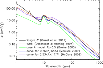
Figure 3: Extinction opacities of the Ormel et al. (2011) dust model “icsgra3” (black) compared to other dust opacities from the literature: grains with thin ice mantles after 10⁵ years of coagulation with a gas density of 10⁶ cm^-3 from Ossenkopf & Henning (1994) (orange); case A model of carbon and silicate dust for R_V=5.5 from Draine (2003) (green); two extinction curves derived for star-forming regions by McClure (2009), one for $0.76<A_{J}<2.53$ (blue), and one for $2.53<A_{J}<17.71$ (purple).

We used dust opacities from Ormel et al. (2011) to account for larger, icy grains (as opposed to the small grains made of amorphous silicates typically found in the interstellar medium). We adopted their dust model that includes graphite grains without ice coating and ice-coated silicates, with a size distribution that assumes growth of aggregates for $3\times 10^{5}$ years, when grains have grown up to 3 $\mu$m in size (“icsgra3”). Particle sizes range from 0.1 to 3 $\mu$m, with a number density that is roughly proportional to $a^{-2.3}$ (where $a$ is the particle radius). Figure 3 shows our adopted opacities compared to different ones found in the literature. The opacities from Draine (2003) assume a mixture of small carbonaceous and amorphous silicate grains. Including larger and icy grains broadens the 10 $\mu$m silicate feature (which is mostly due to the libration mode of water ice) and causes additional absorption at 3 $\mu$m and in the 40-60 $\mu$m range (all mostly due to the presence of water ice). The mid-IR opacities of the “icsgra3” dust model are similar to the ones determined by McClure (2009) for star-forming regions and also to those used by Tobin et al. (2008) to model an edge-on Class 0 protostar; in the mid- to far-IR, they resemble the opacities of Ossenkopf & Henning (1994), which are often used to model embedded sources. In Figure 3, we show model ‘OH5’ from Ossenkopf & Henning (1994), which is listed as the fifth model in their Table 1 and corresponds to grains with thin ice mantles after 10⁵ years of coagulation and a gas density of 10⁶ cm^-3. We could not use the ‘OH5’ opacities for our model grid, since that opacity law does not include scattering properties (which are required by the Whitney Monte Carlo radiative transfer code). Other authors have modified the ‘OH5’ dust to include the scattering cross section and extend the opacities to shorter and longer wavelengths (Young & Evans, 2005; Dunham et al., 2010).

4.1 Model Parameters

There are 3040 models in the grid; they cover 8 values for the total (i.e., intrinsic) luminosity, 4 disk radii, 19 envelope infall rates (which correspond to envelope densities), and 5 cavity opening angles. Each model is calculated for 10 different inclination angles, from 18.2° to 87.2°, in equal steps in $\cos(i)$ (starting at 0.95 and ending at 0.05), resulting in 30,400 different model SEDs. The values for the various model parameters are listed in Table 2. Since there are a large number of parameters that can be set in the Whitney radiative transfer models, we focused on varying those parameters that affect the SED the most, leaving the other parameters at some typical values. For example, we assumed a stellar mass of 0.5 $M_{\odot}$, a disk mass of 0.05 $M_{\odot}$, and an envelope outer radius of 10,000 AU. The stellar mass enters the code in two ways. First, it is needed to relate the density of the envelope to the infall rate (see Equation 1 below). Since we fit the density of the envelope, the infall rate plays no role in the best-fit envelope parameters; any stellar mass can be chosen to determine the infall rate for a given best-fit envelope density. Second, the stellar mass is combined with the stellar radius and disk accretion rate to set the disk accretion luminosity. Given that the accretion luminosity is the actual parameter that influences the SED, it does not matter which of the three factors is varied. For simplicity and reasons described below, we varied the disk accretion rate and the stellar radius, but left the stellar mass constant, to achieve different values for this component of the luminosity.

The total luminosity for each system consists of the stellar luminosity (derived from a 4000 K stellar atmosphere model), the accretion luminosity resulting from material accreting through the disk down to the disk truncation radius, and the accretion luminosity from the hot spots on the stellar surface, where the accretion columns, which start at the magnetospheric truncation radius, land (these columns are not included in the modeled density distribution, since they do not contain dust and do not have a source of opacity in the radiative transfer models). Typically, the accretion luminosity from the hot spots is much larger than the disk accretion luminosity; in our models, the former is about a factor of 9 larger than the latter. We chose three different stellar radii, 0.67, 2.09, and 6.61 $R_{\odot}$ (with the same stellar temperature), resulting in three different stellar luminosities. Since both components of the accretion luminosity depend on the disk accretion rate, choosing a total of eight different disk accretion rates (three for the 0.67 $R_{\odot}$ star, two for the 2.09 $R_{\odot}$ star, and three for the 6.61 $R_{\odot}$ star) results in eight values for the total luminosity used in the grid (see Table 2). The input spectrum produced by the central protostar depends on the relative contributions from the intrinsic stellar luminosity (which peaks at 0.7 $\mu$m) and the accretion luminosity (which is radiated primarily in the UV). In the models, it can be altered to some degree by choosing different combinations of the disk accretion rate and stellar radius (the former affects only the accretion luminosity, while the latter affects both the stellar and accretion luminosity). However, the effect of the input spectrum on the output SED is negligible. Consequently, we cannot reliably measure the relative contributions of stellar and accretion luminosity through our SED fits. Instead, we adjusted the particular values for the stellar radius and disk accretion rate to set the values of the total luminosity.

For our model grid, we chose four values for the disk outer radius, which we set equal to the centrifugal radius ($R_{c}$). In a TSC model, the centrifugal radius is the position in the disk where material falling in from the envelope accumulates; due to envelope rotation, material from the envelope’s equatorial plane lands at $R_{c}$, while material from higher latitudes falls closer to the star. The disk could extend beyond $R_{c}$, but in our models it ends at $R_{c}$. In this work, we use the terms “disk (outer) radius” and “centrifugal radius” interchangeably. The primary effect of $R_{c}$ is to set the rotation rate of the infalling gas and thereby determine the density structure of the envelope (Kenyon et al., 1993).

Table 2: Model Parameters

Parameter	Description	Values	Units
Stellar Properties
$M_{\ast}$	Stellar mass	0.5	$M_{\odot}$
$T_{\ast}$	Stellar effective temperature	4000	K
$R_{\ast}$	Stellar radius	0.67, 2.09, 6.61	$R_{\odot}$
Disk Properties
$M_{disk}$	Disk mass	0.05	$M_{\odot}$
$R_{disk}$	Disk outer radius	5, 50, 100, 500	AU
A	Radial exponent in disk density law	2.25	$\cdots$
B	Vertical exponent in disk density law	1.25	$\cdots$
$\dot{M}_{disk,1}$	Disk-to-star accretion rate for $R_{star}$=0.67 $R_{\odot}$	0, $1.14\times 10^{-8}$, $5.17\times 10^{-8}$	$M_{\odot}$ yr-1
$\dot{M}_{disk,2}$	Disk-to-star accretion rate for $R_{star}$=2.09 $R_{\odot}$	$3.67\times 10^{-7}$, $1.63\times 10^{-6}$	$M_{\odot}$ yr-1
$\dot{M}_{disk,3}$	Disk-to-star accretion rate for $R_{star}$=6.61 $R_{\odot}$	$1.14\times 10^{-5}$, $5.15\times 10^{-5}$, $1.66\times 10^{-4}$	$M_{\odot}$ yr-1
$R_{trunc}$	Magnetospheric truncation radiusa	3	$R_{\ast}$
$f_{spot}$	Fractional area of the hot spots on the starb	0.01	$\cdots$
Envelope Properties
$R_{env}$	Envelope outer radiusc	10,000	AU
$\rho_{1000}$	Envelope density at 1000 AUd	0.0, 1.19 $\times 10^{-20}$, 1.78 $\times 10^{-20}$, 2.38 $\times 10^{-20}$,	g cm-3
		5.95 $\times 10^{-20}$, 1.19 $\times 10^{-19}$, 1.78 $\times 10^{-19}$,	g cm-3
		2.38 $\times 10^{-19}$, 5.95 $\times 10^{-19}$, 1.19 $\times 10^{-18}$,	g cm-3
		1.78 $\times 10^{-18}$, 2.38 $\times 10^{-18}$, 5.95 $\times 10^{-18}$,	g cm-3
		1.19 $\times 10^{-17}$, 1.78 $\times 10^{-17}$, 2.38 $\times 10^{-17}$,	g cm-3
		5.95 $\times 10^{-17}$, 1.19 $\times 10^{-16}$, 1.78 $\times 10^{-16}$	g cm-3
$R_{c}$	Centrifugal radius of TSC envelope	$=R_{disk}$	AU
$\theta$	Cavity opening angle	5, 15, 25, 35, 45	degrees
$b_{cav}$	Exponent for cavity shapee (polynomial)	1.5	$\cdots$
$z_{cav}$	Vertical offset of cavity wall	0	AU
Derived Parameters
$L_{\ast}$	Stellar luminosityf	0.1, 1, 10	$L_{\odot}$
$L_{tot}$	Total luminosity (star + accretion)g	0.1, 0.3, 1.0, 3.1, 10.1, 30.2, 101, 303	$L_{\odot}$
Parameters for Model SEDs
$i$	Inclination angle	18.2, 31.8, 41.4, 49.5, 56.7,	degrees
		63.3, 69.5, 75.6, 81.4, 87.2	degrees
	Aperture radii for model fluxesh	420, 840, 1260, 1680, …, 10080	AU

Note. — The dust opacities used for these models are those called “icsgra3” from Ormel et al. (2011).

^a This radius applies to the gas. The inner disk radius for the dust is equal to the dust destruction radius. The scale height of the disk at the dust sublimation radius is set to the hydrostatic equilibrium solution.

^b The hot spots are caused by the accretion columns that reach from the magnetospheric truncation radius to the star.

^c The inner envelope radius is set to the dust destruction radius.

^d The actual input parameter for the Whitney code is the envelope infall rate, which can be derived from $\rho_{1000}$ using Equation (2). The first six $\rho_{1000}$ values correspond to envelope infall rates of 0, $5.0\times 10^{-8}$, $7.5\times 10^{-8}$, $1.0\times 10^{-7}$, $2.5\times 10^{-7}$, and $5.0\times 10^{-7}$ $M_{\odot}$ yr^-1; the other values can be similarly deduced.

^e The cavity walls are assumed to have a polynomial shape; no material is assumed to lie inside the cavity. Also, the ambient density (outside the envelope) is 0.

^f The three values of $L_{\ast}$ correspond to the three different stellar radii.

^g The total luminosities combine the stellar luminosities and the accretion luminosities (which depend on $\dot{M}_{disk}$).

^h For each model, the emitted fluxes are calculated for 24 apertures ranging from 420 to 10080 AU, in steps of 420 AU.

The largest number of parameter values in our grid is for the envelope infall rate. The envelope infall rate used as an input in the Whitney code sets the density of the envelope for a given mass of the protostar. Since the SED depends on the density of the envelope (and not directly on the infall rate, which is only inferred from the density and the acceleration due to gravity from the central protostar), in this work we report a reference envelope density instead of the envelope infall rate as one of our model parameters. For the TSC model, the envelope infall rate $\dot{M}_{env}$ and the reference density at 1 AU in the limit of no rotation ($R_{c}$=0) are related as follows (see Kenyon et al., 1993):

$$\rho_{1}=5.318\times 10^{-14}\left(\frac{\dot{M}_{env}}{10^{-5}M_{\odot}\,\mathrm{yr}^{-1}}\right)\left(\frac{M_{\ast}}{1\,M_{\odot}}\right)^{-1/2}\mathrm{g}\,\mathrm{cm}^{-3},$$ (1)

where $M_{\ast}$ is the mass of the central protostar, which is assumed to be 0.5 $M_{\odot}$ in our model grid. The density distribution in the envelope follows a power law, $\rho\propto r^{-3/2}$, at radii larger than the centrifugal radius, $R_{c}$, but then flattens as a result of the rotation of the envelope. The density reported by $\rho_{1}$ assumes a spherically symmetric envelope with a $-3/2$ power-law exponent valid down to the smallest radii, and it is higher than the angle-averaged density of a rotating envelope at 1 AU. To quote densities that are closer to actual values found in the modeled rotating envelopes (which have $R_{c}$ values ranging from 5 to 500 AU), we report $\rho_{1000}$, the density at 1000 AU for a $\rho\propto r^{-3/2}$ envelope with a 0.5 $M_{\odot}$ protostar:

$$\rho_{1000} = \rho_{1}\left(\frac{1}{1000}\right)^{3/2}$$ (2)

$$= 2.378\times 10^{-18}\left(\frac{\dot{M}_{env}}{10^{-5}M_{\odot}\,yr^{-1}}\right)\mathrm{g}\,\mathrm{cm}^{-3}.$$

Thus, the range of reference densities probed in our model grid, from $1.2\times 10^{-20}$ to $1.8\times 10^{-16}$ g cm^-3 (see Table 2), would correspond to envelope infall rates from $5.0\times 10^{-8}$ to $7.5\times 10^{-4}$ $M_{\odot}$ yr^-1, assuming $M_{\ast}$=0.5 $M_{\odot}$ (this does not account for a reduction of the infalling mass due to clearing by outflow cavities). In Figure 4, we show the radial density profiles for two TSC models with 5 AU and 500 AU centrifugal radii. The density profiles are azimuthally symmetric and show the flattening of the density distribution inside $R_{c}$ due to envelope rotation. These plots demonstrate that the density $\rho_{1}$ is much higher than the angle-averaged density at 1 AU; $\rho_{1000}$ seems to yield more physical values for the density in the envelope at 1000 AU, even for $R_{c}$ values of 500 AU.

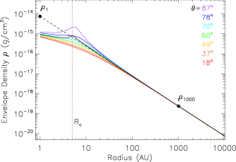
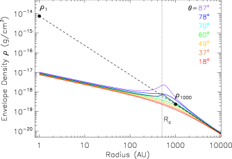
Figure 4: Envelope density versus radius for a model protostar with $\dot{M}_{env}=1.0\times 10^{-6}$ $M_{\odot}$ yr^-1, $M_{\ast}$=0.5 $M_{\odot}$, and $R_{c}$=5 AU (left) and 500 AU (right) to show the difference between the reference densities $\rho_{1}$ and $\rho_{1000}$. The lines with different colors represent radial density profiles for different polar angles $\theta$; the black line represents the angle-averaged density profile (for equations see Whitney et al. 2003a; Adams & Shu 1986). The dashed line represents an $r^{-3/2}$ power law. The vertical dotted line marks the location of the centrifugal radius.

As can be seen from the values of the envelope density in Table 2, there is one set of models with an envelope density of 0. These are models that do not contain an envelope component; the entire excess emission is caused by the circumstellar disk. If an object is best fit by such a model, it would indicate that it is more evolved, having already dispersed its envelope.

Figure 5: Schematic showing the shape of the cavity assumed in our models for three cavity opening angles $\theta$: 5°, 25°, and 45° (from left to right). The cavity walls are defined as a polynomial with exponent 1.5 ($z\propto\tilde{r}^{1.5}$), with $\tilde{r}_{max}=z_{max}\,\tan\theta$, and are shown as solid lines. The outer envelope radius ($R_{env}$) at 10,000 AU is shown with a short-dashed line. The dotted lines show a different definition of the cavity size, where $\tilde{r}_{max}=R_{env}\sin\theta$ and $z_{max}=R_{env}\cos\theta$.

The cavities in our models range from 5° to 45° and are defined such that $z\propto\tilde{r}^{1.5}$, where $\tilde{r}$ and $z$ are the cylindrical coordinates for the radial and vertical direction, respectively, and $\tilde{r}_{max}=z_{max}\,\tan\theta$, with $\theta$ defined as the cavity opening angle that is specified in the parameter file of the Whitney radiative transfer code. In this code, $z_{max}$ is set to the envelope outer radius. Thus, a polynomial-shaped cavity, which is wider at smaller $\tilde{r}$ values and then converges toward the specified opening angle, is somewhat larger than this opening angle at the outer envelope radius (see Figure 5). This effect is most noticeable at larger cavity opening angles, but negligible for small cavities. A different definition of the cavity size, where $\tilde{r}_{max}=R_{env}\sin\theta$ and $z_{max}=R_{env}\cos\theta$ (with $R_{env}$ as the envelope outer radius), results in $z$ values that are a factor of $1/\cos\theta$ larger, and thus the cavity reaches the specified opening angle at the outer envelope radius. For this work, the adopted definition of the cavity opening angle is inconsequential, but it becomes relevant when comparing the results of SED modeling to scattered light images that reveal the actual cavity shape and size. We also note that in our models the cavities are evacuated of material, so there is no dust and gas inside the cavity; in reality, there might be some low-density material left that would add to the scattered light (see Fischer et al., 2014).

Figures 6 to 10 display a few examples of model SEDs from our grid to show the effect of changing those model parameters that influence the resulting SED the most. The inclination angle has a strong effect on the near- and mid-infrared SED (Figure 6). While a low inclination angle results in an overall flat SED in this wavelength region, increasing the inclination angle causes a deeper silicate absorption feature at 10 $\mu$m and a steep slope beyond it. The far-infrared to millimeter SED is not affected by the inclination angle, since emission at these wavelengths does not suffer from extinction through the envelope.

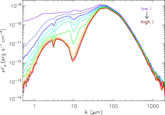
Figure 6: A model from the grid seen at 10 different inclination angles to illustrate the effect of viewing angle on the SED. The model has $L_{tot}$=10.1 $L_{\odot}$, $R_{c}$=50 AU, $\rho_{1000}$=$1.2\times 10^{-18}$ g cm^-3, $\theta$=15°, and is seen at inclination angles 18°, 32°, 41°, 49°, 57°, 63°, 69°, 76°, 81°, and 87° (from top to bottom).

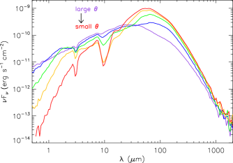
Figure 7: Models from the grid to illustrate the effect of cavity opening angle on the SED. The models have $L_{tot}$=10.1 $L_{\odot}$, $R_{c}$=50 AU, $\rho_{1000}$=$1.2\times 10^{-18}$ g cm^-3, i=63°, but each has a different cavity opening angle: 5° (red), 15° (yellow), 25° (green), 35° (blue), 45° (purple).

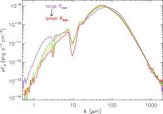
Figure 8: Models from the grid to illustrate the effect of the centrifugal radius ($=R_{disk}$) on the SED. The models have $L_{tot}$=10.1 $L_{\odot}$, $\rho_{1000}$=$1.2\times 10^{-18}$ g cm^-3, $\theta$=5°, i=63°, but different disk radii: 5 AU (red), 50 AU (yellow), 100 AU (green), 500 AU (purple).

The cavity opening angle affects the SED shape at all wavelengths (Figure 7). A small cavity only minimally alters the SED compared to a case without a cavity; there is still a deep silicate absorption at 10 $\mu$m and steep SED slope, but the cavity allows some scattered light to escape in the near-IR. A larger cavity results in higher emission at near- and mid-infrared wavelengths and reduced emission in the far-infrared. The effect of the cavity on the SED would change if a different shape for the cavity walls were adopted. For example, cavities where the outer wall follows the streamlines of the infalling gas and dust evacuate less inner envelope material than our polynomial-shaped cavities, resulting in deeper silicate absorption features and steeper mid-infrared SED slopes for the same cavity opening angle (see Furlan et al., 2014). Thus, our cavity opening angles are tied to our assumed cavity shape.

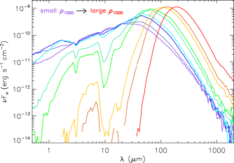
Figure 9: Models from the grid to illustrate the effect of envelope density on the SED. The models have $L_{tot}$=10.1 $L_{\odot}$, $R_{c}$=50 AU, $\theta$=15°, i=63°, but different reference densities $\rho_{1000}$: 0, $2.4\times 10^{-20}$, $1.2\times 10^{-19}$, $2.4\times 10^{-19}$, $1.2\times 10^{-18}$, $2.4\times 10^{-18}$, $1.2\times 10^{-17}$, $2.4\times 10^{-17}$, and $1.2\times 10^{-16}$ g cm^-3 (the peak of the SED moves to longer wavelengths as $\rho_{1000}$ increases).

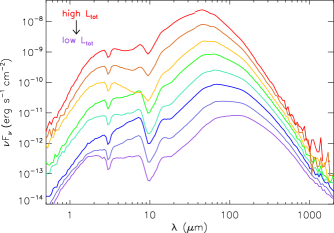
Figure 10: Models from the grid to illustrate the effect of the total luminosity on the SED. The models have $R_{c}$=50 AU, $\rho_{1000}$= $1.2\times 10^{-18}$ g cm^-3, $\theta$=15°, i=63°, but different values for the total luminosity: 0.1, 0.3, 1.0, 3.1, 10.1, 30.2, 101, and 303 $L_{\odot}$ (from bottom to top).

The effect of the centrifugal radius is somewhat similar to those of the cavity opening angle and inclination angle, but less pronounced (Figure 8). Small disk radii imply more slowly rotating, less flattened envelopes and depress the near- and mid-infrared fluxes more than larger disk radii, but even with large disk radii (and more flattened envelopes) there is still sufficient envelope material along the line of sight to cause a pronounced 10 $\mu$m absorption feature. Overall, our models do not directly constrain the size of the disk; the opacity is dominated by the envelope. Furthermore, the flattening of the envelope that is determined by $R_{c}$ has a similar effect on the SED as changing the outflow cavity opening angle.

Changing the envelope density causes shifts in the SED in terms of both wavelength and flux level: the higher the envelope density, the less flux is emitted at shorter wavelengths, and the more the peak of the SED shifts to longer wavelengths (Figure 9). Deeply embedded protostars have SEDs that peak at $\lambda>$ 100 $\mu$m, steep mid-IR SED slopes, and deep silicate absorption features. The effect of the envelope density on the SED is different from that of the inclination angle, especially in the far-IR: while the SED is not very sensitive to the inclination angle in this wavelength region, the ratio of, e.g., 70 and 160 $\mu$m fluxes changes considerably depending on the envelope density.

The total luminosity of the source has an effect on the overall emission level of the protostar, but does not strongly affect the SED shape. The main effect is that the peak of the SED shifts to longer wavelengths as the luminosity decreases ($\lambda_{peak}\propto L^{-1/12}$; Kenyon et al. 1993). Especially when comparing models with $L_{tot}$ values that differ by a factor of a few, the SED shapes are similar (Figure 10). Thus, one could scale a particular model by a factor between $\sim$ 0.5 and 2 and get a good representation of a protostar that is somewhat fainter or brighter, without having to rerun the model calculation with the different input luminosity.

4.2 Model Apertures

The model fluxes are computed for 24 different apertures, ranging from 420 to 10,080 AU in steps of 420 AU (which corresponds to 1″ at the assumed distance of 420 pc to the Orion star-forming complex). For these SED fluxes, no convolution with a PSF is done, and therefore the spatial distribution of the flux is solely due to the extended nature of protostars. Since the envelope outer radius is chosen to be 10,000 AU, the largest aperture encompasses the entire flux emitted by each protostellar system. However, most of the near- and mid-infrared emission comes from smaller spatial scales, so an aperture of about 5000 AU will already capture most of the flux emitted at these wavelengths.

For a more accurate comparison of observed and model fluxes, in each infrared photometric band where we have data available, we interpolate model fluxes from the two apertures that bracket the aperture used in measuring the observed fluxes (4″ for 2MASS, 2$\farcs$4 for IRAC, PSF photometry for MIPS 24 µm, with a typical FWHM of 6″, 9$\farcs$6 for PACS 70 and 100 µm, 12$\farcs$8 for PACS 160 µm). For the IRS data points, we use fluxes interpolated for a 5$\farcs$3 aperture, since the spectra are composed of two segments, SL (5.2-14 µm; slit width of 3$\farcs$6) and LL (14-38 µm, slit width of 10$\farcs$5), and, if any flux mismatches were present, the SL segment was typically scaled to match the LL flux level at 14 µm (see, e.g., Furlan et al., 2008). So, fluxes measured in an aperture with a radius of 5$\farcs$3 roughly correspond to fluxes from a 10$\farcs$6-wide slit.

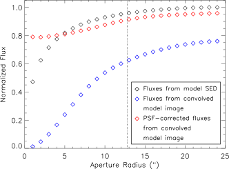
Figure 11: PACS 160 $\mu$m fluxes versus aperture radius derived for a model ($L_{tot}=1.0$ $L_{\odot}$, $R_{c}=100$ AU, $\rho_{1000}=2.378\times 10^{-18}$ g cm^-3, $\theta$=15°, $i=63$°) using different methods. The black symbols represent fluxes from the model SED, the blue symbols fluxes derived using aperture photometry on the model image convolved with the PACS 160 $\mu$m PSF, and the red symbols fluxes derived from the convolved model image and then corrected for PSF losses (see text for details). The maximum flux from the model SED was used to normalize all other fluxes. The dotted line indicates an aperture radius of 12$\farcs$8.

Given that our targets are typically extended and that the near- to mid-infrared data have relatively high spatial resolution, measuring fluxes in small apertures (a few arcseconds in radius) will truncate some of the object’s flux, so it is important to choose similar apertures for the model fluxes. From about 30 to 100 $\mu$m, the model fluxes calculated for smaller apertures are not very different from the total flux (i.e., the flux from the largest aperture), which is a result of the emission profile in the envelope and the lower spatial resolution at longer wavelengths. To check whether extended source emission in the far-infrared might affect the flux we measure in our models, we calculated a small set of model images at 160 $\mu$m, convolved them with the PACS 160 $\mu$m PSF, and compared the fluxes from the model images to those written out for the model SEDs (which we refer to as “SED fluxes”; these are the fluxes from the models in the grid). Model images would be the most observationally consistent way to measure the flux densities, but they are too computationally expensive and would not represent a significant gain.

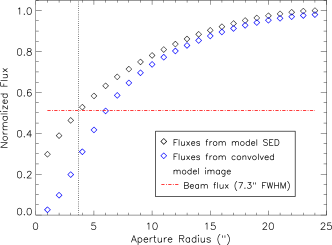
Figure 12: SABOCA (350 $\mu$m) fluxes versus aperture radius derived for the same model as in Figure 11 using different methods. The black symbols represent fluxes from the model SED, the blue symbols fluxes derived using aperture photometry on the model image convolved with a Gaussian PSF, and the red dot-dashed line the beam flux (assuming a beam with a FWHM of 7$\farcs$3). The maximum flux from the model SED was used to normalize all other fluxes. The dotted line indicates an aperture radius of 3$\farcs$65.

In Figure 11 we show the fluxes derived for a particular model at 160 $\mu$m using different methods. The fluxes measured in the convolved model image are lower than the SED fluxes; this is caused by the wide PACS 160 $\mu$m PSF, which spreads flux to very large radii. Since the shape of the PSF is known, we can correct for these PSF losses (assuming a point source and using standard aperture corrections). The fluxes corrected for these PSF losses are very similar to the SED fluxes, typically within $\sim$ 5-10% at apertures larger than 5″. Since our observed fluxes correspond to these PSF-corrected fluxes (we apply aperture corrections to our fluxes measured in a 12$\farcs$8 aperture to account for PSF losses), adopting the SED fluxes from the largest aperture would yield model fluxes that are somewhat too high. Thus, we chose to adopt the SED flux measured in a 12$\farcs$8 aperture as a good approximation for the model flux we would get if we had model images available for all models in the grid and measured aperture-corrected fluxes in these images. We note that in our PACS data, the 160 $\mu$m sky annulus, which extends from 12$\farcs$8 to 25$\farcs$6 (see B. Ali et al. 2016, in preparation), can include extended emission from surrounding material and also some envelope emission. In these cases, we often used PSF photometry to minimize contamination from nearby sources and nebulosity; however, PSF fitting was not used for more isolated sources since the envelopes can be marginally resolved at 160 $\mu$m and thus deviate slightly from the adopted PSF shape.

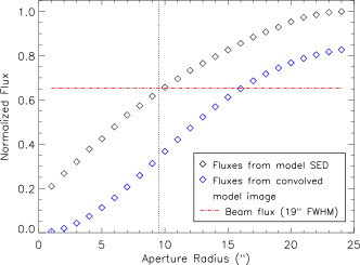
Figure 13: Similar to Figure 12, but for the LABOCA (870 $\mu$m) fluxes. The dotted line indicates an aperture radius of 9$\farcs$5.

For the SABOCA and LABOCA data, beam fluxes were adopted; the FWHM of the SABOCA beam is 7$\farcs$3, while for the LABOCA beam it is 19″. In order to determine which aperture radius corresponds best to beam fluxes, we created a similar set of model images as above at 350 and 870 $\mu$m, convolved them with Gaussian PSFs, and measured fluxes in the model images using different apertures (see Figures 12 and 13, where we show the results for one model). Fluxes measured in the convolved model image are smaller than the SED fluxes, especially at aperture radii smaller than the FWHM of the beam. We find that the beam fluxes for SABOCA and LABOCA are best matched by SED fluxes from apertures with radii half the size of the FWHM of the beam, i.e., 3$\farcs$65 for SABOCA and 9$\farcs$5 for LABOCA (thus, the aperture sizes are the same as the beam FWHM). This is again an idealized situation, since the measured SABOCA and LABOCA beam fluxes also include extended emission (if the source lies on top of background emission), and thus they could be higher than those from the model.

4.3 Effect of External Heating

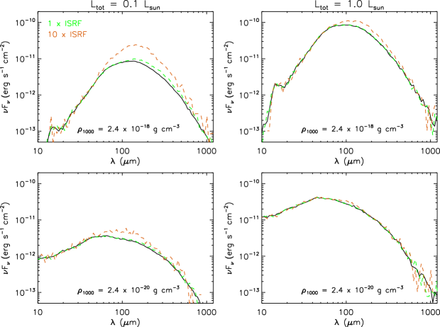
Figure 14: Left: Comparison of models with $L_{tot}$=0.1 $L_{\odot}$, $R_{c}$=100 AU, $\theta$=15°, $\rho_{1000}$=2.4 $\times 10^{-18}$ g cm^-3 (top) or 2.4 $\times 10^{-20}$ g cm^-3 (bottom), $i$=63°, without external heating (black), with external heating by an ISRF equal to that in the solar neighborhood (green, dashed line), and with heating by an ISRF 10 times stronger (orange, dashed line). Right: Similar to the models in the left panels, but these models have $L_{tot}$=1.0 $L_{\odot}$.

In our models, the luminosity is determined by the central protostar and the accretion; no external heating is included. The interstellar radiation field (ISRF) could increase the temperature in the outer envelope regions, thus causing an increase in the longer-wavelength fluxes (e.g., Evans et al., 2001; Shirley et al., 2002; Young et al., 2003). It is expected that external heating has a noticeable effect only on low-luminosity sources ($\lesssim$ 1 $L_{\odot}$), while objects with strong internal heating are not affected by the ISRF. Moreover, the strength of the ISRF varies spatially (Mathis et al., 1983), and thus its effect on each individual protostar is uncertain. Nonetheless, in the following we estimate the effect of external heating on model fluxes by using a different set of models.

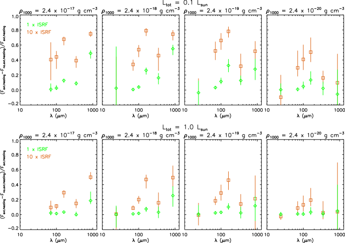
Figure 15: Ratio of the excess emission due to external heating and the emission of the protostar with external heating in different bands, for heating by an ISRF equal to that in the solar neighborhood (green diamonds) and by an ISRF 10 times stronger (orange squares). The vertical lines show the range of flux excess ratios resulting from different viewing angles (inclination angles range from 18° to 87°), while the symbols represent mean values. The top (bottom) panels are for models with $L_{tot}$=0.1 (1.0) $L_{\odot}$. The four columns correspond to the four reference densities probed.

For this model calculation, we used the 2012 version of the Whitney radiative transfer code (Whitney et al., 2013), which allows for the inclusion of external illumination by using the ISRF value in the solar neighborhood from Mathis et al. (1983); to vary the ISRF strength, the adopted value can be scaled by a multiplicative factor and extinguished by a certain amount of foreground extinction. We calculated a small number of models with and without external heating and then compared their far-infrared and submillimeter fluxes. One set of models has $L_{tot}$=0.1 $L_{\odot}$, $R_{c}$=100 AU, $\theta$=15°, and four different reference densities $\rho_{1000}$, ranging from 2.4 $\times 10^{-17}$ g cm^-3 to 2.4 $\times 10^{-20}$ g cm^-3. The other set has the same parameters except for $L_{tot}$, which is 1.0 $L_{\odot}$. We calculated models without external heating, with heating from an ISRF equal to that in the solar neighborhood, and with ISRF heating 10 times the solar neighborhood value. For these models, we did not include any foreground extinction for the ISRF; thus, the ISRF heating in these models can be considered an upper limit – especially the 10-fold increase over the ISRF in the solar neighborhood represents an extreme value. Figure 14 shows a few examples of model SEDs with and without external heating. External heating results in flux increases in the far-IR and sub-mm; as expected, it affects low-luminosity sources more, and its effects are also more noticeable for higher-density envelopes.

For a more quantitative comparison of model fluxes in the far-IR and sub-mm, we computed the fluxes for each model in six different bands, those of MIPS 24 $\mu$m, PACS 70, 100, and 160 $\mu$m, and SABOCA (350 $\mu$m) and LABOCA (870 $\mu$m), using apertures as described in section 4.2. The model fluxes are affected by poorer signal-to-noise ratios at the longest wavelengths, so the 870 $\mu$m fluxes are less reliable. We subtracted the fluxes of the models without external heating ($F_{\rm no.ext.heating}$) from those with external heating ($F_{\rm ext.heating}$) to determine the flux excess due to external heating. The ratios of these excess fluxes and the model fluxes with external heating ($(F_{\rm ext.heating}-F_{\rm no.ext.heating})/F_{\rm ext.heating}$) are shown in Figure 15. Given that these ratios depend on the inclination angle to the line of sight, we show them as average values for all 10 inclination angles as well as the range subtended by all inclination angles. We note overall smaller flux ratios at 350 $\mu$m due to the smaller aperture size chosen in this wave band (see section 4.2).

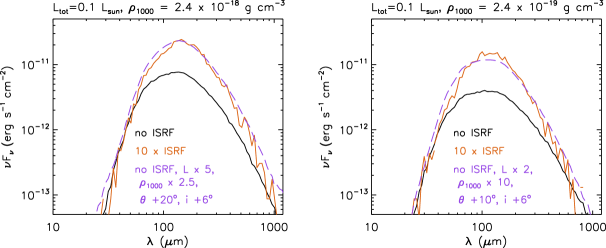
Figure 16: Black and orange lines: SEDs for models with $L_{tot}$=0.1 $L_{\odot}$, $R_{c}$=100 AU, $\theta$=15°, $i$=75°, reference densities $\rho_{1000}$=2.4 $\times 10^{-18}$ g cm^-3 (left) and 2.4 $\times 10^{-19}$ g cm^-3 (right), without external heating (black) and with heating by an ISRF scaled by a factor of 10 (orange). The purple dashed lines show SEDs from our model grid (which does not include external heating) with model parameters changed as indicated in the figure label; these models were chosen to closely match the model SEDs with external heating.

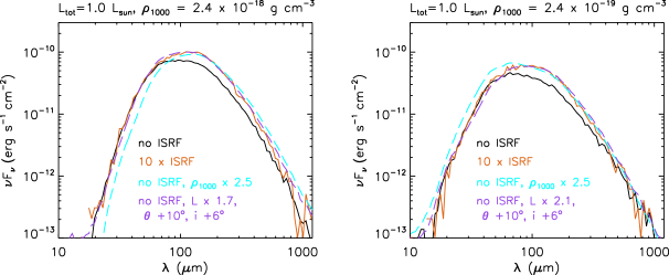
Figure 17: Similar to Figure 16, but for model SEDs with $L_{tot}$=1.0 $L_{\odot}$ (black and orange lines). The light blue and purple dashed lines show SEDs from our model grid (no external heating) with the same model parameters as shown except for a reference density 2.5 times higher (light blue) and $\theta$=25°, $i=$81°, and a higher luminosity (purple).

Our analysis shows that heating by the ISRF results in flux increases in the far-IR and sub-mm that are about a factor of 2-3 higher for envelopes of low-luminosity sources ($L_{tot}$=0.1 $L_{\odot}$) than for those with higher luminosity. Also, the effect of external heating is more noticeable at longer wavelengths (where apertures/beams are also larger) than at shorter ones; given our chosen apertures, the largest effect occurs at 160 and 870 $\mu$m. We also note that the flux increases due to heating by the ISRF are smallest for the lowest $\rho_{1000}$ value probed, 2.4 $\times 10^{-20}$ g cm^-3; at 160 $\mu$m, the flux increase is largest for intermediate envelope densities. Finally, the flux increases in the far-IR and sub-mm are far larger for a solar-neighborhood ISRF scaled by factor of 10 than for an unscaled ISRF; for the $L_{tot}$=0.1 $L_{\odot}$ models, an unscaled ISRF increases the fluxes from a few percent (at $\lesssim$ 100 $\mu$m) to 50% (at 870 $\mu$m), while an ISRF scaled by a factor of 10 increases these fluxes by 30%-75%. Thus, for low-luminosity protostars, up to $\sim$ 75% of a protostar’s 870 $\mu$m flux could be due to external heating, if the environment is dominated by an extremely strong ISRF.

To estimate how the contribution of external heating would modify derived model parameters, in Figures 16 and 17 we compare model SEDs that include external heating by an ISRF 10 times stronger than in the solar neighborhood and model SEDs without this additional heating. For the latter, we used models from our model grid and tried to reproduce the SEDs with external heating. For the models with $L_{tot}$=0.1 $L_{\odot}$, the effect of external heating can be reproduced by increasing the luminosity by factors of a few, increasing $\rho_{1000}$ by up to an order of magnitude, and increasing the cavity opening angle and inclination angle by a small amount. For the $L_{tot}$=1.0 $L_{\odot}$ models, just increasing the reference density by a factor of 2.5 results in a good match to the long-wavelength emission of our externally heated models; however, the shorter-wavelength flux is either under- or overestimated. A better match is achieved with models having the same reference density as the externally heated models, but with slightly larger cavity opening angles and inclination angles, and luminosities about a factor of 2 larger. Thus, if the far-IR and sub-mm fluxes were contaminated by emission resulting from extremely strong external heating, a model fit using models from our grid (which does not include external heating) could overestimate the envelope density by up to an order of magnitude and the luminosity by a factor of 2-5. The cavity opening and inclination angles would also be more uncertain, but not by much. For a more realistic scenario with more modest external heating (which would also include the effect of local extinction), the effect on model parameters would be smaller.

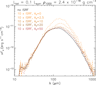
Figure 18: Models with $L_{tot}$=0.1 $L_{\odot}$, $R_{c}$=100 AU, $\theta$=15°, $\rho_{1000}$=2.4 $\times 10^{-18}$ g cm^-3, $i$=63°, without external heating (black), with external heating by an ISRF 10 times stronger than in the solar neighborhood (orange to brown, dashed lines) and different amounts of extinction applied to the ISRF (from $A_{V}=2.5$ to $A_{V}=50$, top to bottom).

For the latter point, we explored the effect of extinction on the ISRF by calculating a few more models with $L_{tot}$=0.1 $L_{\odot}$, $R_{c}$=100 AU, $\theta$=15°, $\rho_{1000}=2.4\times 10^{-18}$ g cm^-3, an ISRF 10 times stronger than that in the solar neighborhood, and $A_{V}$ values for the ISRF of 2.5, 10, 20, and 50. The model SEDs are shown in Figure 18. Compared to ISRF heating without any foreground extinction, already $A_{V}=2.5$ causes a decrease by a factor of 1.5-2 in the overall emission at far-IR wavelengths. With $A_{V}$ of 10 and 20, the far-IR emission decreases by factors of up to $\sim$ 3.5 and 4, respectively, compared to a strong ISRF that is not extinguished. The fraction of excess emission due to external heating at 160 $\mu$m decreases from an average of 0.8 for $A_{V}$=0 (see Figure 15) to 0.6, 0.3, and 0.2 for $A_{V}$=2.5, 10, and 20, respectively. Therefore, considering that typical $A_{V}$ values in Orion are $\sim$ 10-20 mag (Stutz & Kainulainen, 2015), it is likely that the effect of external heating on model parameters of low-luminosity sources does not exceed a factor of $\sim$ 2 in luminosity and $\sim$ 5 in envelope density.

5 Fitting Method

A customized fitting routine determines the best-fit model from the grid for each object in our sample of 330 YSOs (see Sections 2 and 3) using both photometry and, where available, IRS spectroscopy. Ideally, an object has 2MASS, IRAC, IRS, MIPS, PACS, and SABOCA and LABOCA data; in many cases, no submillimeter data are available, and in a few cases the object is too faint to be detected by 2MASS. Of the 330 modeled objects, 40 do not have IRS spectra. As a minimum, objects have some Spitzer photometry and a measured flux value in the PACS 70 $\mu$m band. No additional data from the literature were included in the fits to keep them homogeneous.

In order to reduce the number of data points contained in the IRS spectral wavelength range (such that the spectrum does not dominate over the photometry) and to exclude ice absorption features in the 5-8 µm region and at 15.2 µm that are usually observed, but not included in the model opacities, we rebin each IRS spectrum to fluxes at 16 wavelengths. These data points trace the continuum emission and the 10 and 20 µm silicate features. Also, when rebinning the spectrum, we smooth over its noisy regions, and we scale the whole spectrum to match the MIPS 24 µm flux if a similar deviation is also seen at the IRAC 5.8 and 8 µm bands and is larger than 10%. Figure 19 shows three examples of our IRS spectra with the rebinned fluxes overplotted. Our selection of 16 IRS data points in addition to at most 13 photometric points spread from 1.1 to 870 µm puts more emphasis on the mid-IR spectral region in the fits. This wavelength region is better sampled by observations, most of the emission is thermal radiation from the protostellar envelope and disk (as opposed to some possible inclusion of scattered light or thermal emission from surrounding material at shorter and longer wavelengths, respectively), and it contains the 10 µm silicate feature, which crucially constrains the SED fits. As a result, most models are expected to reproduce the mid-IR fluxes well and might fit more poorly in the near-IR and sub-mm.

Figure 19: Three IRS spectra, one for HOPS 32 (Class 0 protostar; top), one for HOPS 84 (Class I protostar; middle), and one for HOPS 105 (flat-spectrum source; bottom), overlaid with the rebinned data points (filled circles) used by the fitting routine. Note the different flux ranges on the y axis in the three panels and thus the big differences in slopes among the three spectra.

To directly compare observed and model fluxes, we create model SEDs with data points that correspond to those obtained from observations, from both photometry and IRS spectroscopy. For the former, the model fluxes are not only derived from the same apertures as the data (see section 4.2), but also integrated over the various filter bandpasses, thus yielding model photometry. For the latter, the model fluxes are interpolated at the same 16 wavelength values as the IRS spectra.

Since the model grid contains a limited number of values for the total luminosity (eight), but the objects we intend to fit have luminosities that likely do not correspond precisely to these values, we include scaling factors for the luminosity when determining the best-fit model. As long as these scaling factors are not far from unity, they are expected to yield SEDs that are very similar to those obtained from models using the scaled luminosity value as one of the input parameters. The scaling factor can also be related to the distance of the source; for all model fluxes, a distance of 420 pc is assumed, but in reality the protostars in our sample span a certain (presumably small) range of distances along the line of sight. For example, a 10% change in distance would result in a $\sim$ 20% change in flux values (scaling factors of 0.83 or 1.23). Here we report luminosities assuming a distance of 420 pc.

In addition to scaling factors, each model SED can be extinguished to account for interstellar extinction along the line of sight. We use two foreground extinction laws from McClure (2009) that were derived for star-forming regions: one applies to $0.76\leq A_{J}<2.53$ (or $0.3\leq A_{K}<1$), and the other one to $A_{J}\geq 2.53$ (or $A_{K}\geq 1$). For $A_{J}<0.76$, we use a spline fit to the Mathis $R_{V}=5$ curve (Mathis, 1990). Since the three laws apply to different extinction environments, we use a linear combination of them to achieve a smooth change in the extinction law from the diffuse interstellar medium to the dense regions within molecular clouds. Thus, to find a best-fit model for a certain observed SED, the model fluxes $F_{mod}(\lambda)$ are scaled and extinguished as follows:

$$F_{obs}(\lambda)=sF_{mod}(\lambda)10^{-0.4A_{\lambda}},$$ (3)

where $F_{obs}(\lambda)$ and $F_{mod}(\lambda)$ are the observed and model fluxes, respectively, $s$ is the luminosity scaling factor, and $A_{\lambda}$ is the extinction at wavelength $\lambda$. We use three reddening laws, $k_{\lambda}=A_{\lambda}/A_{J}$; by denoting them with the subscripts 1, 2, and 3, $A_{\lambda}$ in the above equation becomes

$$A_{\lambda}=A_{J}k_{1,\lambda}\quad{\rm for}\;A_{J}<0.76$$

$$A_{\lambda}=0.76k_{1,\lambda}+(A_{J}-0.76)k_{2,\lambda}$$

$${\rm for}\;0.76<A_{J}<2.53$$

$$A_{\lambda}=0.76k_{1,\lambda}+2.53k_{2,\lambda}+(A_{J}-2.53)k_{3,\lambda}$$

$${\rm for}\;A_{J}>2.53$$ (4)

Thus, equation 3 can be written as

$$2.5\log(F_{mod}(\lambda)/F_{obs}(\lambda))=A_{J}k_{1,\lambda}-2.5\log(s)$$

$${\rm for}\;A_{J}<0.76$$

$$2.5\log(F_{mod}(\lambda)/F_{obs}(\lambda))-0.76(k_{1,\lambda}-k_{2,\lambda})=$$

$$A_{J}k_{2,\lambda}-2.5\log(s)\quad{\rm for}\;0.76<A_{J}<2.53$$

$$2.5\log(F_{mod}(\lambda)/F_{obs}(\lambda))-0.76k_{1,\lambda}-2.53(k_{2,\lambda}-k_{3,\lambda})$$

$$=A_{J}k_{3,\lambda}-2.5\log(s)\quad{\rm for}\;A_{J}>2.53\qquad$$ (5)

These are linear equations in $A_{J}$, with the left-hand side of the equations as the dependent variables and $k_{\lambda}$ as the independent variable. For each regime of $A_{J}$ values, a best-fit line can be determined that yields $A_{J}$ and $-2.5\log(s)$ from the slope and intercept, respectively, for each model that is compared to the observations.

For each set of model fluxes and observed fluxes, we calculate three linear fits (using linear combinations of the three different extinction laws, as explained above), thus yielding three values for scaling factors and three for the extinction value. If each extinction value is within the bounds of the extinction law that was used and smaller than a certain maximum $A_{J}$ value (which will be discussed below), and the scaling factor is in the range from 0.5 to 2.0, then the result with the best linear fit will be used. However, if some of the values are not within their boundaries, then combinations of their limiting values are explored, and the set of scaling factor and extinction with the best fit is adopted. For example, if a model has fluxes that are much higher than all observed fluxes, the linear fit described above will likely yield very large extinction values and small scaling factors. In this case the fitter would only accept the smallest possible scaling factor (0.5) and the maximum allowed $A_{J}$ value as a solution (which will still result in a poor fit).

For each object, we allowed the model fluxes to be extinguished up to a maximum $A_{J}$ value derived from column density maps of Orion (Stutz & Kainulainen 2015; see also Stutz et al. 2010, 2013; Launhardt et al. 2013 for the methodology of deriving N_H from 160-500 µm maps). We converted the total hydrogen column density from these maps to $A_{V}$ values ($A_{V}$=3.55 $A_{J}$) by using a conversion factor of $1.0\times 10^{21}$ cm^-2 mag^-1 (Winston et al., 2010; Pillitteri et al., 2013). For objects for which no column density could be derived, we set the maximum $A_{J}$ value to 8.45 (which corresponds to $A_{V}=30$).

After returning a best-fit scaling factor and extinction value for each model, each data point is assigned a weight, and the goodness of the fit is estimated with

$$R=\frac{\sum_{i=1}^{N}w_{i}|\ln\left(\frac{F_{obs}(\lambda_{i})}{F_{mod}(\lambda_{i})}\right)|}{N},$$ (6)

where $w_{i}$ are the weights, $F_{obs}(\lambda_{i})$ and $F_{mod}(\lambda_{i})$ are the observed and the scaled and extinguished model fluxes, respectively, and N is the number of data points (see Fischer et al., 2012). Thus, $R$ is a measure of the average, weighted, logarithmic deviation between the observed and model SED. It was introduced by Fischer et al. (2012) since the uncertainty of the fit is dominated by the availability of models in the grid (i.e, the spacing of the models in SED space) and not by the measurement uncertainty of the data, making the standard $\chi^{2}$ analysis less useful. Also, a statistic that measures deviations between models and data in log space more closely resembles the assessment done by eye when comparing models and observed SEDs in log($\lambda F_{\lambda}$) vs. $\lambda$ plots. We set the weights $w_{i}$ to the inverse of the estimated fractional uncertainty of each data point; so, for photometry at wavelengths below 3 µm they are equal to 1/0.1, between 3 and 60 µm they are 1/0.05, at 70 and 100 µm they are 1/0.04, at 160 µm the weight is 1/0.07, and for photometry at 350 and 870 µm they are 1/0.4 and 1/0.2, respectively. For fluxes from IRS spectra the weights are 1/0.075 for wavelength ranges 8-12 µm and 18-38 µm, while they are 1/0.1 for the 5-8 µm and 12-18 µm regions. These IRS weights are also multiplied by 1.5 for high signal-to-noise spectra and by 0.5 for noisy spectra. In this way those parts of the IRS spectrum that most constrain the SED, the 10 µm silicate absorption feature and slope beyond 18 $\mu$m, are given more weight; for high-quality spectra, the weights in these wavelength regions are the same as for the 3-60 µm photometry.

For small values, $R$ measures the average distance between model and data in units of the fractional uncertainty. In general, the smaller the $R$ value, the better the model fit, but protostars with fewer data points can have small $R$ values, while protostars with some noisy data can have larger $R$ values (but still an overall good fit). We find a best-fit model for each object, but we also record all those models that lie within a certain range of $R$ values from the best-fit $R$. These models give us an estimate on how well the various model parameters are constrained (see Section 6.4).

Our model grid is used to characterize the parameters that best describe the observed SED of each object; the $R$ values rank the models for each object and thus can be used to derive best-fit parameters, as well as estimates of parameter ranges. In several instances, better fits could be achieved if the model parameters were further adjusted, for example by testing more values of cavity opening angle or shape, or even changing the opacities (see, e.g., HOPS 68 (Poteet et al., 2011), HOPS 223 (Fischer et al., 2012), HOPS 59, 60, 66, 108, 368, 369, 370 (Adams et al., 2012), HOPS 136 (Fischer et al., 2014), and HOPS 108 (Furlan et al., 2014)). However, for protostars that are well fit with one of the models from the grid or for which the grid yields a narrow range of parameter values, it is unlikely that a more extended model grid would yield much different best-fit parameters. Overall, our model fits yield good estimates of envelope parameters for a majority of the sample, and thus we can analyze the protostellar properties of our HOPS targets in a statistical manner.

6 Results of the Model Fits

The best-fit parameters resulting from our models can be found in Table A1, and Figure A53 shows the SEDs and best fits for our sample. In this section we give an overview of the quality of the fits, the distributions of the best-fit model parameters, both for the sample as a whole and separated by SED class, the parameter uncertainties, and the various degeneracies between model parameters.

6.1 Quality of the Fits

Figure 20: Histogram of the $R$ values of the best fits of the 330 YSOs in the HOPS sample that have Spitzer and Herschel detections.

Figure 21: Histograms of the $R$ values of the best fits shown separately for the three classes of objects (Class 0, I, and flat-spectrum). The three fits with $R>8$ (two Class 0 protostars, one Class I protostar) are not shown.

Figure 20 displays the histogram of $R$ values of the best model fits for the 330 objects in our HOPS sample that have Spitzer and Herschel data (more than two data points at different wavelengths) and are not contaminants (see Section 2). The median $R$ value is 3.10, while the mean value is 3.29. Fitting a Gaussian to the histogram at $R$ $\leq$ 7 yields 3.00 and 2.24 as the center and FWHM of the Gaussian, respectively. The distribution of $R$ values implies that, on average, the model deviates by about three times the average fractional uncertainty from the data. This is not unexpected, given that we fit models from a grid to observed SEDs that span almost three orders of magnitude in wavelength range, with up to 29 data points. The fewer the data points, the easier it is to achieve a good fit; in fact, the eight protostars with $R<1$, HOPS 371, 391, 398, 401, 402, 404, 406, and 409, have SEDs with measured flux values at only 4-5 points. Starting at $R$ values of about 1, $R$ can be used as an indicator of the goodness of fit. However, in some cases a noisy IRS spectrum can increase the $R$ value of a fit that, judged by the photometry alone, does not deviate much from the observed data points. In other cases, mismatches between different data sets, like offsets between the IRAC fluxes and the IRS spectrum, can result in larger $R$ values. These might be interesting protostars affected by variability and are thus ideal candidates for follow-up observations.

When looking at the SED fits in Figure A53 (and the corresponding $R$ values in Table A1), we estimate that an $R$ value of up to $\sim$ 4 can identify a reliable fit (with some possible discrepancies between data and model in certain wavelength regions). When $R$ gets larger than about 5, the discrepancy between the fit and the observed data points usually becomes noticeable; the fit might still reproduce the overall SED shape but deviate substantially from most measured flux values.

In Figure 21, we show the histogram of $R$ values separately for the three main protostellar classes in our sample. The median $R$ value decreases from 3.27 for the Class 0 protostars to 3.18 for the Class I protostars to 2.58 for the flat-spectrum sources. There are 4 Class 0 protostars and 4 Class I protostars with $R$ values between 1.0 and 2.0, but 17 flat-spectrum sources in this $R$ range. These numbers translate to 17% of the flat-spectrum sources in our sample, 4% of the Class 0 protostars, and 3% of the Class I protostars. When examining objects’ $R$ values between 2.0 and 4.0, there are 51 Class 0 protostars (55% of Class 0 protostars in the sample), 91 Class I protostars (73% of the Class I sample), and 74 flat-spectrum sources (73% of the flat-spectrum sample).

Thus, close to 90% of flat-spectrum sources are fit reasonably well ($R$ values $<$ 4), representing the largest fraction among the different classes of objects in our sample. This could be a result of their source properties being well represented in our model grid, but also lack of substantial wavelength-dependent variability (see, e.g., Günther et al. 2014), which, if present, would make their SEDs more difficult to fit. About three-quarters of Class I protostars also have best-fit models with $R<4$; this fraction drops to about two-thirds for the Class 0 protostars. The latter group of objects often suffers from more uncertain SEDs due to weak emission at shorter wavelengths (which, e.g., results in a noisy IRS spectrum); they might also be more embedded in extended emission, such as filaments, which can contaminate the far-IR to submillimeter fluxes. Another factor that could contribute to poor fits is their presumably high envelope density, which places them closer to the limit in parameter space probed by the model grid. Overall, 75% of the best-fit models of the protostars in our sample have $R<4$.

When examining the SED fits of objects with $R$ values larger than 5.0, several have very noisy IRS spectra (HOPS 19, 38, 40, 95, 164, 278, 316, 322, 335, 359). In a few cases the measured PACS 100 and 160 $\mu$m fluxes seem too high compared to the best-fit model (e.g., HOPS 189), which could be an indication of contamination by extended emission surrounding the protostar.

Of particular interest are objects where variability likely plays a role in a poor fit. As mentioned in Section 3, variability among protostars is common; we found in Appendix B that about 5% of our targets display noticeable ($\gtrsim$ 50%) mismatches between the IRS, IRAC, and MIPS fluxes that could be due to intrinsic variability. The SED fits of objects for which the flux mismatches between IRS and IRAC and between IRS and MIPS are different are particularly affected, since in that case we did not scale the IRS spectrum to match the MIPS 24 $\mu$m flux. HOPS 228 exemplifies such a case: there is a clear discrepancy between the IRAC and IRS fluxes (a factor of 2.1-2.7) and also between MIPS 24 $\mu$m and IRS (a factor of 0.8); even though the fit gives more weight to the IRS data, they are not fit well, especially the silicate absorption feature. The $R$ value of 5.74 for the fit of HOPS 228 reflects the discrepant data sets and poor fit. HOPS 223 is another case where the IRS fluxes do not match the shorter-wavelength data (they are more than an order of magnitude larger); however, it is a known FU Ori source (see Fischer et al., 2012), and the SED presented here contains both pre- and post-outburst data. The model fit is very poor, which can also be gauged by the $R$ value of 8.41.

There are also objects with overall good fits whose SEDs show discrepancies that may be signs of variability or contamination. For example, for the Class I protostar HOPS 71 the IRAC fluxes are a factor of 1.8-2.4 lower than the IRS fluxes in the 5-8 $\mu$m region, and also the MIPS flux is about 20% lower. The best-fit model ($R=3.63$) fits the SED extremely well beyond about 6 $\mu$m, with some discrepancy at shorter wavelengths. There is a source just 11″ from HOPS 71 that is detected in 2MASS and Spitzer data, but not by PACS; this object, HOPS 72, is likely an extragalactic object (see Appendix D.2.2) that could contaminate the IRS fluxes. Thus, in this case, wavelength-dependent contamination by a companion could explain the discrepancies observed in the SED.

Another example is HOPS 124, which is a deeply embedded Class 0 protostar. For this object, the mismatch between IRS and IRAC and MIPS fluxes decreases with increasing wavelength (from a factor of 2.5 to a factor of 1.4); for the SED fit, the IRS spectrum was scaled by 0.7 to match the MIPS 24 $\mu$m flux. As with HOPS 71, there is a nearby source that could contaminate some of the fluxes, especially at shorter wavelengths: HOPS 125, a flat-spectrum source, lies 9.8″ from HOPS 124 and is brighter than HOPS 124 out to $\sim$ 20 $\mu$m, but then much fainter at longer wavelengths. The best-fit model of HOPS 124 ($R=2.43$) matches the mid- to far-IR photometry and also most of the IRS spectrum well.

As an example of a probably variable flat-spectrum source, HOPS 132 has IRAC fluxes that lie a factor of 1.3-1.7 above those of IRS and a MIPS 24 $\mu$m flux that is a factor of 0.6 lower. It does not have a close companion; the nearest HOPS source, HOPS 133, is 27″ away. The IRS spectrum was not scaled, and since the SED fitter gave more weight to the spectrum, it is fit well, but the IRAC photometry is underestimated and the MIPS photometry overestimated. Nonetheless, the $R$ value of the best fit is 2.87.

Overall, the SED fits of objects that are likely variable or suffer from some contamination are less reliable, but it is not always clear from the $R$ value of the best fit. The SED fitting procedures assume that the protostars are not variable, so when large mismatches between different data sets are present, the fit will appear discrepant with at least some of the observed data points, but the $R$ value would not end up particularly high if, e.g., the IRS spectrum was fit exceptionally well. However, given the data sets we have for these protostars, our SED fits will still yield the best possible estimate for the protostellar parameters describing these systems.

6.2 Overview of Derived Parameters

The histogram of best-fit $\rho_{1000}$ values (which is the density of the envelope at 1000 AU; see Section 4.1) is shown in Figure 22. The median value of the distribution amounts to $5.9\times 10^{-19}$ g cm^-3; this corresponds to a $\rho_{1}$ value of $1.9\times 10^{-14}$ g cm^-3. There is a spread in values: 69 objects have densities $\rho_{1000}$ smaller than $5.0\times 10^{-20}$ g cm^-3 (6 of them have actually no envelope), 89 fall in the $5.0\times 10^{-20}$ to $5.0\times 10^{-19}$ g cm^-3 range, 96 are between $5.0\times 10^{-19}$ and $5.0\times 10^{-18}$ g cm^-3, 60 between $5.0\times 10^{-18}$ and $5.0\times 10^{-17}$ g cm^-3, and 16 have $\rho_{1000}$ values larger than $5.0\times 10^{-17}$ g cm^-3.

Figure 22: Histogram of the envelope reference density $\rho_{1000}$ of the best fits for the 330 targets in our sample.

Figure 23: Histogram of the envelope mass within 2500 AU derived for the best fits for the 330 targets in our sample.

We also calculated the envelope mass ($M_{env}$) within 2500 AU for the best-fit models (see Figure 23 for their distribution). The 2500 AU radius is close to half the FWHM of the PACS 160 $\mu$m beam at the distance of Orion (i.e., $\sim$ 6″), and thus roughly represents the spatial extent over which we measure the SEDs. This envelope mass is determined from the integrated envelope density of our best-fit models, with allowances made for outflow cavities, and thus only valid in the context of our models. The median envelope mass within 2500 AU amounts to 0.029 $M_{\odot}$. The majority of protostars have model-derived masses in the inner 2500 AU of their envelopes around 0.1 $M_{\odot}$; just 22 objects have $M_{env}$ ($<$ 2500 AU) larger than 1.0 $M_{\odot}$. Of the 330 modeled objects, 291 have $M_{env}$ ($<$ 2500 AU) smaller than 0.5 $M_{\odot}$ (6 of these 291 objects have no envelope).

Figure 24: Histogram of the total luminosities of the best fits for the 330 targets in our sample.

Figure 25: Histogram of the disk radii of the best fits for the 330 targets in our sample.

Figure 26: Histogram of the cavity opening angles of the best fits for the 330 targets in our sample.

Figure 27: Histograms of the envelope reference density $\rho_{1000}$ (left), the total luminosity (middle), and the disk radius (right) of the best fits grouped by cavity opening angles.

Figure 24 contains the histogram of the total luminosities derived from the best-fit models. These luminosities consist of the stellar, disk accretion, and accretion shock components. The median total luminosity amounts to 3.02 $L_{\odot}$, while the values cover four orders of magnitude, from 0.06 $L_{\odot}$ (for HOPS 336) to 607 $L_{\odot}$ (for HOPS 288 and 361). Since the minimum and maximum values for the total luminosity in our grid amount to 0.1 and 303.5 $L_{\odot}$, respectively, and our scaling factors range from 0.5 to 2.0, our fitting procedure can return best-fit luminosities that range from 0.05 to 607 $L_{\odot}$. Thus, two protostars are reaching the upper limit allowed for total luminosities in our grid; it is possible that even better fits could be achieved by increasing the luminosity further.

From the distribution of best-fit outer disk radii in Figure 25, it is apparent that most protostars are fit by small disks whose radius is only 5 AU. Since the outer disk outer radius is the centrifugal radius in our models, infalling material from the envelope tends to accumulate close to the star for most sources. Thus, the disk radius is tied to the envelope structure; a small centrifugal radius implies higher envelope densities at smaller radii and a less flattened envelope structure. The median disk radius is 50 AU, but the number of objects with disk radii $\geq$ 50 AU is roughly evenly split among the values of 50, 100, and 500 AU.

The distribution of best-fit cavity opening angles is displayed in Figure 26. Most protostars seem to have either very small (5°) or very large (45°) cavities; the median value is 25°. When dividing the envelope densities by cavity opening angle (see Figure 27, left column), differences emerge: the distributions of $\rho_{1000}$ values are significantly different when comparing objects with $\theta$=5° and $\theta\geq$35°, objects with $\theta$=15° and $\theta$ $\geq$ 25°, and objects with $\theta$=25° and $\theta$=45°. The Kolmogorov-Smirnov (K-S) tests yield significance levels that these subsamples are drawn from the same parent population of $\lesssim$ 0.015. Thus, there seems to be a difference in the distribution of envelope densities among the best-fit models with smaller cavity opening angles and those with larger cavities. Protostars with larger cavities ($\geq$ 35°) tend to have higher envelope densities (their median $\rho_{1000}$ values are about an order of magnitude larger compared to objects with cavities $\leq$ 15°).

Figure 27 (middle column) also shows the distribution of total luminosities for the different cavity opening angles. The only significant difference can be found for the $\theta$=5° histogram as compared to the histograms for larger $\theta$ values (K-S test significance level $\lesssim$ 0.03); the luminosities of models with $\theta$=5° have a different distribution, and also their median value is 1.45 $L_{\odot}$, as compared to $\sim$ 3-5 $L_{\odot}$ for the models with larger cavities. So, protostars with small cavities seem to have lower total luminosities.

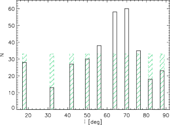
Figure 28: Histogram of the inclination angles of the best fits for the 330 targets in our sample. The green dashed histogram represents the distribution of uniformly (randomly) distributed inclination angles.

The distribution of centrifugal radii for different cavity opening angles (right column in Figure 27) shows that, independent of cavity size, most objects have $R_{disk}$ = 5 AU. However, the distribution among the four different disk radii becomes flatter for the largest cavity opening angles; the histograms for $\theta$=35° and $\theta$=45° are very similar (K-S test significance level of 0.98). There is also no significant difference (K-S test values $>$ 0.075) between the $\theta$=15° and $\theta$=25° histograms and between the $\theta$=5° and $\theta\geq$ 35° histograms. The distributions of disk radii for the other cavity opening angles are all different from one another (K-S test significance levels $<$ 0.015). Overall, Figure 27 shows that protostars best fit by models with large cavity opening angles are also fit by models with higher envelope densities and larger centrifugal radii.

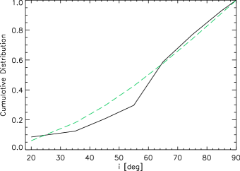
Figure 29: Cumulative distribution of the inclination angles of the best fits, normalized by the total number of fits (solid line), compared to the cumulative probability of finding an inclination angle below a given value for randomly distributed inclinations (green dashed line).

In Figure 28, we show the distribution of the inclination angles for the best-fit models. There is a clear concentration of models in the 60°$-$70° range; the median inclination angle is 63°. This median value is close to 60°, which is where the probability for isotropically distributed inclination angles reaches 50% (i.e., the probability of observing an inclination angle less than 60° is the same as the probability of observing i$>$60°). However, the details of the distributions differ. The cumulative probability of finding an inclination angle less than a certain value, $i_{c}$, is $1-\cos(i_{c})$, assuming a random distribution of inclination angles. For inclination angles $i_{1}$ and $i_{2}$, the probability for $i_{1}<i<i_{2}$ is $\cos(i_{1})-\cos(i_{2})$. Thus, since the inclination angles in our model grid were chosen to be equally spaced in $\cos(i)$ (there are five values $<$60° and five values $>$60°), one would expect a flat distribution in Figure 28 if the best-fit inclination angles were randomly distributed (see the green dashed histogram). However, we find a distribution peaked at 63° and 70°. This can also be seen in Figure 29, where we compare our observed cumulative distribution of inclination angles to that of randomly distributed ones. Our distribution shows a deficit at inclination angles below 60° and is just slightly higher at large inclination angles. A K-S test of the two distributions yields a 5.6% chance that they are drawn from the same parent distribution.

Figure 30: Histograms of the envelope reference density $\rho_{1000}$ (left), total luminosity (middle), and cavity opening angles (right) of the best fits divided by bins of inclination angles.

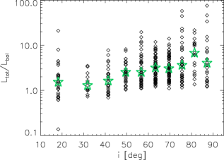
Figure 31: Ratio of the total luminosity from the best fits and the bolometric luminosity derived from the observed SEDs versus the inclination angle (left) and foreground extinction (right) of the best fits. In the left panel, the open stars represent the median ratios at each inclination angle. In the right panel, the open circles represent the median ratios for eight bins in $A_{V}$ values, represented by the horizontal lines bisecting each circle.

To examine whether the distribution of envelope parameters changes with inclination angle (which could imply a degeneracy), Figure 30 shows the reference envelope density $\rho_{1000}$, the total luminosity, and the cavity opening angle binned by three ranges of inclination angles. None of the three model parameters show a significantly different distribution for any of the inclination bins (K-S test significance levels are $\gtrsim$ 0.1, except for the cavity opening angles for the lowest and middle inclination range, for which the K-S test significance value is 0.02). The median $\rho_{1000}$ values for the $i=$18°–41°, 49°–63°, and 69°–87° inclination bins are all $5.9\times 10^{-19}$ g cm^-3. Even though not shown in Figure 30, the objects whose best-fit model does not include an envelope are only found at $i\geq$ 49°. It is noteworthy that protostars with the highest envelope densities do not have inclination angles in the 69°–87° range; it is not clear whether this is an observational bias, whether our observed sample does not contain high-density, edge-on protostars, or whether this is due to biases in the fitting procedure and/or model grid. The median values for the total luminosity do not differ by much for the different bins of inclination angle, increasing from 2.9 to 4.1 $L_{\odot}$ from the lowest to the middle inclination range and then decreasing to 2.0 $L_{\odot}$ for the highest inclination angles. The few protostars with very high $L_{tot}$ values have large inclination angles ($i\geq$ 49°). Finally, the distribution of cavity opening angles is quite similar for different ranges in inclination, except for a somewhat larger number of $\theta=$ 45° values at intermediate inclination angles. Half the objects in the $i=$18°–41° and 69°–87° inclination bins have $\theta\leq$ 15° (with the most common value 5°), while almost half the objects at intermediate inclination angles have $\theta\geq$ 35° (the most common value is 45°).

In Figure 31, we show ratios of the total and bolometric luminosities as a function of inclination angle and foreground extinction ($i$ and $A_{V}$ are adopted from the best model fits). The total luminosity is the intrinsic luminosity from the best-fit model of each object, while the bolometric luminosity is derived by integrating the fluxes of the observed SED. It is expected that $L_{tot}$ is higher than $L_{bol}$ for objects seen at higher inclination angles, since for these objects a large fraction of the emitted flux is not directed toward the observer (and thus deriving bolometric luminosities from observed fluxes will underestimate the intrinsic source luminosity). Conversely, objects seen more face-on should have lower $L_{tot}$ values compared to $L_{bol}$. Our data and model fits yield $L_{tot}$ values that are usually higher than the $L_{bol}$ values measured from the SED; the discrepancy is larger for the more highly inclined sources. The median $L_{tot}/L_{bol}$ ratio is 1.5 for protostars with inclination angles in the 18°–41° range, 2.5 for the i=49°–63° range, and 3.5 for inclination angles $\geq$ 69°. The fact that $L_{tot}>L_{bol}$ even for $i=$18°–41° could be related to the typically smaller cavity opening angles for this range of inclination angles (see Figure 30); less flux, especially at shorter wavelengths, is detected since the opacity along the line of sight is still high due to the small cavities.

Foreground extinction also plays a role in increasing the $L_{tot}$/$L_{bol}$ ratio. The median ratio of these luminosities increases from 1.8 for the $A_{V}$= 0-5 mag range to 5.0 for $A_{V}$=25-30; it decreases somewhat for the next $A_{V}$ bin, but reaches 5.9 at $A_{V}$=40-50 (the 23 objects with $A_{V}>$ 50, not shown in Figure 31, have a median $L_{tot}$/$L_{bol}$ ratio of 8.2). Among the 22 objects with best-fit $A_{V}$ values of 0-5 mag and inclination angles $\leq$ 50°, only four have $L_{tot}/L_{bol}$ ratios that are larger than 1.5 (they are HOPS 57, 147, 199, and 201; in most cases the model overestimates the near-IR emission).

6.3 Envelope Parameters for Different SED Classes

Figures 32–37 divide the histograms of the best-fit reference density $\rho_{1000}$, inclination angle, cavity opening angle, total luminosity, disk radius, and foreground extinction, respectively, by protostar class. As explained in Section 3, we divided our targets into Class 0, Class I, flat-spectrum, and Class II objects based on their mid-infrared (4.5-24 µm) spectral index and bolometric temperature (see also Table A1). Thus, Class 0 and I protostars have a spectral index $>$ 0.3, and Class 0 protostars have $T_{bol}$ values $<$ 70 K, but, as mentioned in Section 3, there are a few protostars whose spectral index or $T_{bol}$ value places them very close to the transition region between Class 0 and I or between Class I and flat spectrum. Given that our sample contains just eleven Class II pre-main-sequence stars, we did not include them in the following histograms; they will be discussed in section 7.2.3.

Figure 32: Histograms of the envelope reference density $\rho_{1000}$ of the best fits for the different SED classes.

The distributions of reference densities (Figure 32) are different for all SED classes; none are consistent with being drawn from the same parent population (K-S test significance level $<$ 0.01). Overall, Class 0 protostars have higher envelope densities than Class I and flat-spectrum sources; the median $\rho_{1000}$ values decrease from 5.9 $\times 10^{-18}$ g cm^-3 to 2.4 $\times 10^{-19}$ g cm^-3 to 1.2 $\times 10^{-19}$ g cm^-3 for these three groups. The lower and upper quartiles for $\rho_{1000}$ are 1.8 $\times 10^{-18}$ and 1.8 $\times 10^{-17}$ g cm^-3 for the Class 0 protostars, and 2.4 $\times 10^{-20}$ and 1.2 $\times 10^{-18}$ g cm^-3 for the Class I and flat-spectrum objects. We will discuss some implications of these differences in derived envelope densities in section 7.2.

Figure 33: Histograms of the inclination angles of the best fits for the different SED classes.

Figure 34: Histograms of the cavity opening angles of the best fits for the different SED classes.

Figure 35: Histograms of the total luminosity of the best fits for the different SED classes.

For the inclination angles (Figure 33), the distributions are significantly different for all protostellar classes, too (K-S test significance level $\ll$ 0.01). As was shown in Figure 28, a random distribution of inclination angles would result in equal numbers of protostars at each value; there is a deficit of Class 0 and Class I protostars at $i\lesssim$ 60°, and there are also few Class I protostars and hardly any flat-spectrum sources at the highest inclination angles. The median inclination angle is highest for Class 0 protostars (70°), then decreases somewhat for Class I protostars (63°) and even more for flat-spectrum sources (57°). Similar to the envelope density, the median inclination angle decreases as one progresses from Class 0 to flat-spectrum sources.

In the distributions of cavity opening angles (Figure 34), significant differences can be found between Class 0 and Class I protostars and between Class I protostars and flat-spectrum sources (K-S test significance level $\ll$ 0.01). The median cavity opening angle is 15° for the Class I protostars, but 25° for the other two classes. About 40% of Class I protostars have $\theta$=5°, while the distribution among the different cavity opening angles is flatter for the other two object classes. The large fraction of Class I protostars with small cavities could be the result of degeneracy in model parameters (see section 7.2) or our assumptions on envelope geometry (see section 7.4). There are notably few flat-spectrum sources with a 5° cavity opening angle; most of them have cavity opening angles of 15° or 45°.

When comparing the total luminosities for the different SED classes (Figure 35), the distribution of $L_{tot}$ values is different for the Class 0 protostars when compared to the other two classes (K-S test significance level $<$ 0.015), but similar for Class I protostars and flat-spectrum sources. The median total luminosity for Class 0 protostars is 5.5 $L_{\odot}$, compared to 2.0 $L_{\odot}$ for Class I protostars and 3.0 $L_{\odot}$ for flat-spectrum sources. Both Class 0 and I protostars cover close to the whole range of $L_{tot}$ values in the model grid ($\sim$ 0.06-600 $L_{\odot}$), while flat-spectrum sources span a more limited range, from 0.1 to 316 $L_{\odot}$.

Figure 36: Histograms of the disk radii of the best fits for the different SED classes.

Figure 37: Histograms of the foreground extinction of the best fits for the different SED classes.

The distribution of centrifugal radii for the whole sample showed a preference for 5 AU (see Figure 25). When separating the best-fit disk radii by protostellar class (Figure 36), it is clear that the trend for small centrifugal radii is driven by the flat-spectrum sources and also Class I protostars. The fraction of Class 0 protostars with $R_{disk}$= 5 AU is 17%; it increases to 46% and 73% for Class I protostars and flat-spectrum sources, respectively. The median disk radius decreases from 100 AU for Class 0 protostars to 50 AU for Class I protostars to 5 AU for flat-spectrum sources. All three histograms are significantly different from one another (K-S test significance level $\ll$ 0.001). The unexpectedly small centrifugal radii for Class I protostars and flat-spectrum sources could point to parameter degeneracies (see section 7.2) or the need to revise certain model assumptions (see section 7.4).

Finally, the distribution of best-fit foreground extinction values (Figure 37) is similar for all three object classes (K-S test significance level $>$ 0.03). Even the median values are close: $A_{V}$=9.2 for Class 0 protostars, $A_{V}$=8.9 for Class I protostars, and $A_{V}$=10.1 for flat-spectrum sources. Most objects are fit with relatively low foreground extinction values. As can be seen from Figure 38, the majority of protostars have best-fit $A_{V}$ values well below the maximum $A_{V}$ values determined from column density maps, which were used as the largest allowed $A_{V}$ values for the SED fitter. The ratio of model-derived $A_{V}$ to observationally constrained maximum $A_{V}$ is lower than 0.5 for about 60% of the sample.

Figure 38: Foreground extinction values $A_{V}$ from the best-fit models versus the maximum $A_{V}$ value determined from column density maps of Orion. The dashed line indicates where the two $A_{V}$ values are equal.

Figure 39: Best-fit $\rho_{1000}$ values versus the foreground extinction for the different SED classes. Note that there are a few objects at $A_{V}>75$, but they are not shown for overall clarity of the figure.

Figure 40: Best-fit $\rho_{1000}$ values versus inclination angle for the different SED classes. The size of the plotting symbol increases with the number of objects having the same ($i$, $\rho_{1000}$) combination; the legend in the leftmost panel shows which symbol size corresponds to which number of objects.

In Figure 39, we plot the reference densities $\rho_{1000}$ versus the foreground extinction for Class 0, Class I, and flat-spectrum sources. As was already seen in Figure 37, the extinction along the line of sight is similar for all three classes, with most objects in the $A_{V}\sim$ 0-30 regime. Class 0 protostars, which have higher envelope densities, tend to have lower $A_{V}$ values from foreground extinction; the highest-density envelopes are spread among a wide range of $A_{V}$ values. The result is similar for Class I protostars. Flat-spectrum sources display a range in envelope densities at various foreground extinction values; the lowest-density envelopes typically have $A_{V}<20$. Thus, foreground extinction does not seem to affect the classification of protostars. This result is also supported by the statistical analysis of Stutz & Kainulainen (2015), who found that, for $A_{V}$ values up to 35, the misclassification of a Class I protostar as a Class 0 protostar due to foreground extinction (which results in a lower $T_{bol}$) is low.

Table 3: Median Best-Fit Parameter Values for the Three Protostellar Classes

Parameter	Class 0	Class I	Flat-spectrum
$L_{tot}$	5.5 $L_{\odot}$	2.0 $L_{\odot}$	3.0 $L_{\odot}$
$\rho_{1000}$	5.9 $\times 10^{-18}$ g cm-3	2.4 $\times 10^{-19}$ g cm-3	1.2 $\times 10^{-19}$ g cm-3
$\theta$	25°	15°	25°
$R_{disk}$	100 AU	50 AU	5 AU
$i$	70°	63°	57°
$A_{V}$	9.2	8.9	10.1

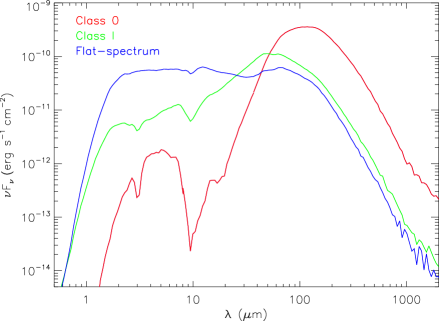
Figure 41: Model SEDs for Class 0 protostars (red), Class I protostars (green), and flat-spectrum sources (blue) with parameter values equal to the median values for each SED class (see Table 3).

We found differences in the best-fit envelope densities and inclination angles for the various protostellar classes. The result that Class 0 protostars tend to have larger inclination angles and envelope densities compared to Class I and flat-spectrum objects can also be seen in Figure 40. There are very few Class 0 protostars with low inclination angles; most have relatively high density and $i>$60°. Class I protostars are best fit by somewhat lower inclination angles than Class 0 protostars and also lower $\rho_{1000}$ values. The best-fit reference density for Class I protostars decreases as the inclination angle increases; thus, higher-density protostars are typically classified as Class I protostars only if they are not seen at close to edge-on orientations. Flat-spectrum sources are spread out in density–inclination space, but intermediate inclination angles and low envelope densities are common. There is a relatively large number of objects at $i=$18° and a deficit of objects at high inclination angles. The highest-density flat-spectrum sources are seen at inclination angles $<$ 50°, while the lower-density objects cover almost the full range of inclination angles.

The median parameter values we determined from the best fits for the Class 0, Class I, and flat-spectrum sources (see Table 3) can be used to show representative median SEDs for each protostellar class. In Figure 41, we show model SEDs whose parameter values are equal to the median values found for each of the three protostellar classes. It is apparent that the large envelope density and higher inclination angle for Class 0 protostars cause a deep absorption feature at 10 $\mu$m and a steeply rising SED in the mid- and far-IR, with a peak close to 100 $\mu$m. In Class I protostars, the SED is less steep and peaks at a shorter wavelength than the median SED of Class 0 protostars. Flat-spectrum sources show the strongest near-IR emission of the three protostellar classes; their median SED is very flat out to 70 $\mu$m, but at longer wavelengths it is very similar in shape and flux level to that of Class I protostars.

6.4 Estimating Parameter Uncertainties

Figure 42: Mode of the inclination angle of all models that lie within 0.5, 1.0, 1.5, and 2 of the best-fit $R$ value (from left to right) versus the best-fit inclination angle for all 330 objects in our sample. Note that for each data point, small random offsets in the x and y direction have been applied to avoid overlap. Also, when two or more parameter values had the same frequency within a $\Delta R$ bin (i.e., not a unique mode value), we computed the average of these values and used it for the mode. The dashed line indicates where the mode and best-fit value are equal.

Figure 43: Mode of the total luminosity of all models that lie within 0.5, 1.0, 1.5, and 2 of the best-fit $R$ value (from left to right) versus the best-fit total luminosity for all 330 objects in our sample.

Given that the $R$ values are a measure of the goodness of fit in units of the fractional uncertainty, we can use models that lie within a certain range of the best-fit $R$ value to estimate uncertainties for the various model parameters. For each modeled HOPS target, we tabulated the model parameters for all those models that lie within a difference of 0.5, 1.0, 1.5, and 2.0 of the best-fit $R$. We then computed the mode (i.e., the value with the highest frequency) for the inclination angle, total luminosity, $\rho_{1000}$, cavity opening angle, outer disk radius, and $A_{V}$ in each of the $\Delta R$ bins for each object. For any given protostar, the models in each $\Delta R$ bin span certain ranges in parameter values; while the modes do not capture the full extent of these ranges, they convey the most common value within each parameter range. The farther away a mode is from the best-fit value, the more poorly constrained the model parameter. Conversely, if a mode of a certain parameter is close to or matches the best-fit value, especially for $\Delta R=$ 1.5 or 2, that particular model parameter is well constrained. In Figures 42 to 47 we plot the mode versus the best-fit value for six model parameters and four $\Delta R$ bins for all 330 targets in our sample. The larger $\Delta R$, the larger the spread in modes is expected to be for each parameter value.

For example, Figure 42 shows that even when considering all models with an $R$ value of up to 2 larger than the best-fit $R$ ($\Delta R=$ 2), the inclination angle for objects with a best-fit $i$ of 18° is well constrained; most modes lie at $i=$ 18°, too, and only a few modes can be found at larger inclination angles. However, objects with best-fit $i$ values of 32° or 41° typically can also be fit by models with lower inclination angles (the majority of modes lies below the line where mode and best-fit value are equal). Inclination angles $\gtrsim$ 63° are better constrained, since their modes mostly lie at high inclination angle values, but there are protostars with modes of $i=$18°, too.

Figure 44: Similar to Figure 42, but for the reference density $\rho_{1000}$.

Figure 45: Similar to Figure 42, but for the cavity opening angle.

Figure 46: Similar to Figure 42, but for the outer disk radius ($=R_{c}$).

Figure 47: Similar to Figure 43, but for the foreground extinction.

The modes for the total luminosity (Figure 43) show a small spread for models within $\Delta R$=0.5, but the spread increases as $R$ increases, with some objects displaying up to an order of magnitude in variation of $L_{tot}$. As illustrated in Figure 44, the reference density $\rho_{1000}$ is usually well constrained; however, as $R$ increases, the modes of the $\rho_{1000}$ values are often lower than the best-fit values. For the cavity opening angle (Figure 45), many models up to $\Delta R$=2 have modes of $\theta$=45°, independent of the best-fit value. Similarly for the centrifugal radius (Figure 46), $R_{disk}$=500 AU is a common mode. For all four disk radii, the modes tend to be larger than the best-fit values; in particular, objects with a best-fit $R_{disk}$ of 5 AU have a very uncertain disk radius. In general, it looks like our models do not constrain the disk radius and cavity opening angle well. The foreground extinction (Figure 47) displays a certain range of modes for each best-fit value, but objects with $A_{V}\lesssim$ 20 typically have more reliable $A_{V}$ values from their model fits.

Figures 42 to 47 allow us to gauge general trends between best-fit values and modes for different model parameters. For results on individual objects, we refer to Appendix C, where we show plots of the difference between the modes and the best-fit values of the major model parameters for all modeled HOPS targets. In this way it is possible to estimate which models are better constrained and thus which objects have more reliable SED fits. In addition, in Appendix C we also include contour plots of $R$ values for different pairs of model parameters for a few targets to illustrate typical parameter degeneracies, which also contribute to parameter uncertainties.

7 Discussion

7.1 Deriving Envelope Parameters from a Model Grid

We compared a grid of TSC models to each target by ranking the models using a statistic, $R$, which measures the deviation between observed and model fluxes in logarithmic space. We did not model each source by further adjusting the model parameters, but instead identified the best-fit SED from our model grid. Thus, we are bound by the range and sampling of parameters chosen for the grid, and while we constructed the grid with the aim of covering the typical parameter space for protostars, it is limited to discrete values. It is likely that many protostars have best-fit parameters that would fall between those sampled by the grid, and a few objects could have parameter values that lie beyond the limits set by the grid. In addition, TSC models are axisymmetric and have mostly smooth density and temperature profiles, and they do not include external heating. They assume a rotating, infalling envelope with constant infall rate and with the gravitational force dominated by the central protostar, but the true envelope structure is likely more complex. The models would not apply to the collapse of a cloud in an initial filamentary or sheet-like geometry or to multiple systems with, e.g., more than one outflow cavity (e.g., Hartmann et al., 1996; Tobin et al., 2012).

Despite the relatively simple models that we use, many of the observed SEDs are fit remarkably well: 75% of the fits have $R<4$. In those cases, the continuum traced by the IRS spectrum, the silicate absorption feature at 10 $\mu$m, and the PACS fluxes are all accurately reproduced by the model. Even many flat-spectrum sources, which often do not display any spectral features in the mid-infrared and have an overall flat SED out to 30 or 70 $\mu$m, often have models that fit them very well. About 75% of Class I protostars and $\sim$ 70% of Class 0 protostars have $R<4$, while close to 90% of flat-spectrum sources have $R$ values in this range. This validates the choice of parameter values for our model grid. Additional constraints, like limits on foreground extinction or information on the inclination and cavity opening angles from scattered light images or mapping of outflows, would allow us to further test and refine the models. We have used limits on the extinction in our analysis. Although Hubble Space Telescope (HST) scattered light images have been used to constrain models for one HOPS protostar (Fischer et al., 2014), scattered light images are not available for many of our targets. We therefore chose to focus on fitting the SEDs of all of our targets in a uniform way to a well-defined set of models. Future studies will incorporate scattered light images and compare the results to those from the SED fits (J. Booker et al. 2016, in preparation).

The best-fit models from our grid for the HOPS targets both reproduce the SEDs and yield estimates for their protostellar parameters, mostly envelope properties. However, these are not necessarily unique fits to the data for three reasons. First, there are degeneracies in the model parameters; increasing the envelope density or inclination angle, or decreasing the cavity opening angle or disk radius, results in a steeper mid-IR SED slope and deeper silicate features. Each of these parameters affects the SED differently (just the general trends are the same), and the best fit for each object tries optimizing them. The next best fit, however, could be a different combination of these parameters, especially if the SED is not well constrained by observations (see Section 6.4). Second, although the TSC models reproduce the observed SEDs, other models with different envelope geometries may also be able to fit the same SEDs. The modeling presented here is only valid in the context of the TSC models of single stars, and the resulting derived properties are only valid within that framework. Last, neglecting external heating could result in overestimated envelope densities and luminosities, with the most noticeable effects ($\rho_{1000}$ and $L_{tot}$ too large by factors of a few) on low-luminosity sources exposed to strong radiation fields (see Section 4.3). From the distribution of best-fit $L_{tot}$ values, we estimate that $\sim$ 20% of HOPS targets in our sample could be affected by external heating. Even though we do not know the strength of external heating for each protostar, it is likely that external heating would only result in relatively small changes in the derived envelope parameters for these protostars.

7.2 Envelope Properties and SED Classes

When comparing envelope parameters sorted by SED classes, we found that envelope densities and inclination angles decrease from the sample of Class 0 protostars through that of Class I protostars to that of flat-spectrum objects. The former is likely an evolutionary effect, while the latter confirms the results of previous work (e.g., Evans et al., 2009) that the inclination angle has an important effect on the SED and that the evolutionary state of an object cannot be derived from SED slopes alone. Thus, there is a difference between the “stage” and “class” of an object (Robitaille et al., 2006); Stage 0 and I objects are characterized by substantial envelopes, Stage II objects are surrounded by optically thick disks, with possibly some remnant infalling envelopes, and Stage III objects have optically thin disks.

In general, the trends we see among model parameters are a consequence of the definition of a protostar based on its SED: in order to be classified as a Class 0 or I object, a protostar is required to have a near- to mid-infrared SED slope larger than 0.3. A protostellar model with a small cavity opening angle, small centrifugal radius, and/or high inclination angle will generate such an SED, since it increases the optical depth along the line of sight. Models with a large cavity will only yield a rising SED in the 2$-$40 $\mu$m spectral range if their envelope density is large or the inclination angle is relatively high.

We find that Class 0 protostars can be best fit not only by very high envelope densities but also moderately high envelope densities and large inclination angles. The bolometric temperature, which is used to separate Class 0 from Class I protostars, is inclination dependent; some Class I protostars are shifted to the Class 0 regime if they are viewed more edge-on. The higher-density Class I protostars tend to have lower inclination angles (but still $>$ 50°); thus, their evolutionary stage could be similar to more embedded protostars that are seen edge-on and classified as Class 0 protostars. Conversely, some Class 0 objects with large inclination angles, but lower envelope densities, could be in a later evolutionary stage than typical Class 0 protostars. Similarly, Class I protostars with large $i$ and low $\rho_{1000}$ values could be edge-on Stage II objects (whose infrared emission is dominated by a disk). Finally, low-inclination Stage 0 and I protostars can appear as a flat-spectrum sources (Calvet et al., 1994).

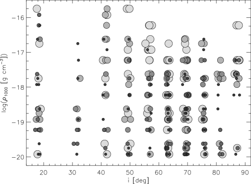
Figure 48: Best-fit $\rho_{1000}$ values versus inclination angle with the cavity size indicated by the different symbol sizes and gray shades: symbols become larger and lighter colored with increasing cavity size (5°, 15°, 25°, 35°, 45°). A small random offset in the x direction has been applied to each data point to prevent too much overlap.

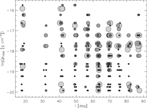
Figure 49: Similar to Figure 48, but with the outer disk radius indicated by the different symbol sizes and gray shades: symbols become larger and lighter colored with increasing disk radius (5, 50, 100, 500 AU).

Nevertheless, the observed trend in envelope densities suggests that the variations in the observed SEDs track, in great part, an evolution toward lower envelope densities and lower infall rates. Assuming a certain mass for the central star, the reference density in our models can be used to infer an envelope infall rate ($\dot{M}_{env}\propto\rho_{1000}\sqrt{M_{\ast}}$). As mentioned in section 4.1, this infall rate is model dependent and therefore tied to the assumptions of the models. With this in mind, the median $\rho_{1000}$ values for the Class 0, Class I, and flat-spectrum protostars in our sample correspond to envelope infall rates of $2.5\times 10^{-5}$, $1.0\times 10^{-6}$, and $5.0\times 10^{-7}$ $M_{\odot}$ yr^-1, respectively, for a 0.5 $M_{\odot}$ star. Using a more realistic assumption of larger stellar mass for more evolved protostars, the infall rates for Class I and flat-spectrum protostars would be larger than these values by a factor of a few. However, just larger stellar masses cannot explain the large decrease of a factor of 50 in the median envelope density from Class 0 to flat-spectrum protostars; to achieve such a decrease with a constant infall rate of $2.5\times 10^{-5}$ $M_{\odot}$ yr^-1, the stellar mass would have to increase by a factor of 2500. Thus, within the context of our model fits, we can conclude that, as envelopes become more tenuous, the infall rates also decrease.

Other trends are also apparent. Class 0 protostars and flat-spectrum sources show a relatively flat distribution of cavity opening angles. On the other hand, the best fit for a large fraction of Class I protostars (40%) results in $\theta$=5°. This could point to a degeneracy in the models, since protostars with small cavity opening angles tend to have lower envelope densities (and also lower total luminosities); thus, the smaller cavity partly compensates for the lower opacity resulting from the lower envelope density (see also Figure 48).

Even though our models do not yield reliable disk properties, we can make a statement about the difference in the best-fit centrifugal radii (or $R_{disk}$), which are tied to the structure of the rotating envelope given by the model fits. It should be noted that the centrifugal radii set a lower limit to the disk radii, since disks may spread outward due to viscous accretion. Most Class I protostars and flat-spectrum sources are fit with a centrifugal radius of just 5 AU. Since the smallest centrifugal radius in our model grid is 5 AU and the next value is 50 AU, we can state that, except for Class 0 protostars, most protostars in our sample have $R_{disk}<50$ AU, and some might even have $R_{disk}<$ 5 AU.

Small disks of those sizes have been observed; radio interferometry of the multiple protostellar system L1551 IRS 5 shows disks whose semi-major axes are $\lesssim$ 20 AU (Rodríguez et al., 1998; Lim & Takakuwa, 2006). However, there is a degeneracy between the centrifugal radius and the envelope density; for protostars with low envelope densities, the small centrifugal radius can compensate the decrease in opacity by concentrating more material closer to the star. As can be seen in Figure 49, most protostars with $R_{disk}=$ 5 AU also have lower envelope densities. Inclination angle also plays a role; protostars seen at $i>$ 80° typically have larger centrifugal radii. In addition, our envelope models include outflow cavities, which allow some of the mid-IR radiation to escape. In order to generate model SEDs with silicate absorption features and steep mid-IR slopes at low to intermediate inclination angles, a lower $R_{disk}$ value is needed. We will discuss the potential implications of the small cavity sizes and $R_{c}$ values for Class I protostars and flat-spectrum sources in Section 7.4.

7.2.1 The Most Embedded Protostars

Among the Class 0 protostars, there are protostars in the earliest evolutionary stages, when the envelope is massive and the protostar still has to accrete most of its mass. Stutz et al. (2013) identified 18 protostars with very red mid- to far-infrared colors ($\log(\lambda F_{\lambda}(70)/\lambda F_{\lambda}(24))$ $>$ 1.65), of which 11 were newly identified (see Table D1). Tobin et al. (2015) added an additional object. These protostars were named PACS Bright Red sources (PBRs) by Stutz et al. (2013); they are HOPS 169, 341, 354, 358, 359, 372, 373, 394, 397-405, 407, and 409. Based on their steep 24-70 $\mu$m SEDs and large submillimeter luminosities, they were interpreted as the youngest protostars in Orion with very dense envelopes.

From our best-fit models to the SEDs of the PBRs, we derive a median $\rho_{1000}$ value of 1.2 $\times$ 10^-17 g cm^-3, which is twice as high as the median value of all the Class 0 protostars in our sample. These fits also result in a median envelope mass within 2500 AU of 0.66 $M_{\odot}$ for the PBRs, but the individual objects cover a large range, from 0.07 to 1.83 $M_{\odot}$. The median total luminosity amounts to 5.6 $L_{\odot}$ (with a range from 0.6 to 71.0 $L_{\odot}$), which is very similar to the median $L_{tot}$ value for the Class 0 protostars in our sample. Most PBRs (14 out of 19 protostars) are fit by models with large inclination angles ($i\geq$ 70°), but, as shown in Stutz et al. (2013), high inclination alone cannot explain the redness of the PBRs. Thus, our models confirm the results of Stutz et al. (2013) that the PBRs are deeply embedded and thus likely among the youngest protostars in Orion.

7.2.2 Flat-spectrum Sources

A particularly interesting group of protostars that are not easy to categorize are the flat-spectrum sources. They are thought to include objects in transition between Stages I and II, when the envelope is being dispersed (Greene et al., 1994). In particular, those with low envelope densities could be more evolved protostars, or they could be protostars that started out with more tenuous envelopes. On the other hand, flat-spectrum sources could also be highly inclined disk sources (see Crapsi et al., 2008), or protostars surrounded by dense envelopes, but seen close to face-on (Calvet et al., 1994). This type of misclassification could have a large effect on the lifetimes of the earlier protostellar stages and thus on the timeline of envelope dispersal. Among the 330 HOPS targets in our sample, we identified 102 flat-spectrum sources based on their flat ($-0.3$ to $+0.3$) spectral index from 4.5 to 24 $\mu$m (or 5-25 $\mu$m in a few cases). Thus, they compose a fairly large fraction of our protostellar sample. Of these 102 objects, 47 have a negative spectral index and 55 have one between 0 and $+0.3$; 41 have a spectral index between $-0.1$ and 0.1, which results in a very flat mid-infrared SED.

Despite a flat SED slope between 4.5 and 24 $\mu$m, many flat-spectrum sources display a weak silicate emission or absorption feature at 10 $\mu$m, which may indicate the presence of a very tenuous infalling envelope or may be the result of the viewing geometry. Some SEDs are very flat out to 100 $\mu$m, others have negative spectral slopes beyond 40 $\mu$m, and again others a rising SED from the mid- to the far-IR. There are also objects with more pronounced absorption features due to not only silicates but also ices, as are typically found in Class 0 and I protostars, but also edge-on disks (see HOPS 82, 85, 89, 90, 92, 129, 150, 200, 210, 211, 281, 304, 331, and 363). Only two flat-spectrum sources have prominent silicate emission features, and their SEDs are reminiscent of protoplanetary disks (see HOPS 187 and 199). Thus, flat-spectrum sources likely include objects of a variety of evolutionary stages.

Figure 50: Median best-fit $\rho_{1000}$ values at each inclination angle for the Class 0 and I protostars (squares) and the flat-spectrum sources (circles) in our sample.

The latter conclusion can also be drawn when analyzing the distribution of envelope reference densities and inclination angles for flat-spectrum sources. In Figure 40, we showed that flat-spectrum sources typically have intermediate inclination angles and lower envelope densities. To compare their properties more directly to Class 0 and I protostars, in Figure 50 we show the median best-fit $\rho_{1000}$ value at each best-fit inclination angle; it is larger for Class 0 and I protostars than for flat-spectrum sources at all inclination angles. For Class 0 and I protostars, the median $\rho_{1000}$ value is highest at intermediate inclination angles, decreases at larger inclination angles, and then increases again for $i>$ 80°. For flat-spectrum sources, the median $\rho_{1000}$ value is relatively flat over the 18°–63° region but has its peak value at $i=$41°; it decreases for larger inclination angles. The only flat-spectrum source with a best-fit inclination angle of 81°, HOPS 357, has a very low envelope density (the lowest value for this parameter in the model grid), and its spectrum displays a deep silicate absorption feature.

Overall, this shows that, while a range of envelope densities and inclination angles can explain flat-spectrum sources, their envelope densities are typically lower than for Class 0 and I protostars. The higher-density objects are seen at low to intermediate inclination angles, while only the lowest-density objects are seen closer to edge-on. Some of the high-density flat-spectrum sources could actually be more embedded protostars (Stage 0 objects) seen face-on (which would be classified as Class 0 objects if seen at larger inclination angles). Thus, in terms of envelope evolution, they include a diverse group of objects.

Figure 51: Best-fit $\rho_{1000}$ values versus the 350 $\mu$m fluxes for the Class 0 and I protostars (left) and the flat-spectrum sources (right) in our sample. Detections at 350 $\mu$m are shown with diamonds, while upper limits are shown with arrows. The histograms show the distribution of best-fit $\rho_{1000}$ values for sources with a 350 $\mu$m flux measurement (thick solid line) and with 350 $\mu$m upper limits (shaded area).

Figure 52: Similar to Figure 51, but for the 870 $\mu$m fluxes.

We note that even though we find that flat-spectrum sources have in general lower envelope densities than Class 0 and Class I objects, their best fit does include an envelope in almost all cases; just 3 of the 102 flat-spectrum sources are best fit without an envelope. This seems to contradict recent findings by Heiderman & Evans (2015), who found that only about 50% of flat-spectrum sources were actually protostars surrounded by envelopes. This could be partly explained by different criteria used to select flat-spectrum sources; in the Heiderman & Evans (2015) sample, flat-spectrum sources are selected by their extinction-corrected 2-24 $\mu$m spectral index (see also Evans et al. 2009; Dunham et al. 2013), while our sample uses a flat 4.5-24 $\mu$m spectral index. Moreover, in their study Heiderman & Evans (2015) detected the presence of an envelope via HCO⁺ emission, and they found that almost all sources detected in the sub-mm are also detected in HCO⁺ (but the opposite does not always hold). For our sample of Orion protostars, we find that 75% of Class 0+I protostars observed with SABOCA (350 $\mu$m) are detected, while only 47% of flat-spectrum sources have detections. For LABOCA observations (870 $\mu$m), these two fractions amount to 41% and 21%, respectively. Thus, we find that flat-spectrum sources have a $\sim$ 50% lower sub-mm detection rate than Class 0+I protostars. Flat-spectrum sources without sub-mm detections would likely also not display HCO⁺ emission and thus would be considered as protostars without envelopes by Heiderman & Evans (2015).

To compare how our submillimeter detections correlate with the presence of an envelope, in Figures 51 and 52 we show the derived best-fit reference envelope densities as a function of 350 or 870 $\mu$m fluxes for the combined Class 0+I sample and the flat-spectrum sources. We also differentiate the distribution of envelope densities between measured flux values and upper limits; at 870 $\mu$m, the upper limits are often cases where the sources are not detected due to confusion with bright, spatially varying emission. We find that even protostars with upper limits at 350 and 870 $\mu$m are best fit with an envelope; however, the envelope density is lower for objects with upper limits in the sub-mm. This is especially evident for Class 0+I protostars; for flat-spectrum sources, the distributions of envelope densities for sub-mm detections and upper limits show significant overlap. Four times as many flat-spectrum sources have upper limits instead of detections at 870 $\mu$m, but their derived $\rho_{1000}$ values span almost the full range of values. Furthermore, the median $\rho_{1000}$ value of 1.19 $\times 10^{-19}$ g cm^-3 for sources without detections is relatively close to the median value of 5.95 $\times 10^{-19}$ g cm^-3 for the sources with 870 $\mu$m detections. Thus, our model fits do not rely on sub-mm detections to yield a best fit with an envelope; in most cases the near- to far-IR SED is sufficient to constrain the properties of the envelope.

7.2.3 Sources without an Envelope and Class II Objects

Among the six objects whose best-fit SED required no envelope ($\rho_{1000}$ value of 0), three are flat-spectrum sources (HOPS 47, 187, 265), two are Class II pre-main-sequence stars (HOPS 113, 293), and one is a Class I protostar (HOPS 232). The low 70 $\mu$m fluxes of HOPS 47 and 265 constrained the best model to one without an envelope. The SED of HOPS 187 looks like that of a transitional disk, which are disks with gaps or holes in their inner regions (see Espaillat et al. 2014 and references therein). If HOPS 187 were a transitional disk, it would not have an envelope. HOPS 232 has a rising SED over the mid-IR spectral range; its best fit requires no envelope, but an edge-on disk with a high accretion luminosity.

It would be expected that the SEDs of Class II objects can be best fit by a model that does not include an envelope. This is the case for HOPS 113 and 293. Of the nine remaining Class II objects in our sample, four have very low envelope densities ($\rho_{1000}\sim(1-2.5)\times 10^{-20}$ g cm^-3; HOPS 22, 26, 98, 283), while five have $\rho_{1000}$ between $6.0\times 10^{-20}$ and $1.8\times 10^{-19}$ g cm^-3 (HOPS 184, 201, 222, 272, 277). The SEDs of HOPS 22, 184, and 201 are similar to those of transitional disks, with some silicate emission at 10 $\mu$m and a rising SED between about 13 and 20 $\mu$m. The best-fit models require some envelope emission to fit the long-wavelength data. HOPS 222, 272, and 277 lie close to the border between a Class II pre-main-sequence star and a flat-spectrum source based on their 4.5-24 $\mu$m spectral index, and therefore they could have some envelope material left, despite being classified as Class II objects.

Overall, of the 330 YSOs in our sample, 319 were classified as either Class 0, Class I, or flat-spectrum protostars based on their SEDs. However, four of them are best fit without an envelope. Conversely, of the 11 Class II objects in our sample, nine are best fit with an envelope; however, three of these might be transitional disks. Thus, based on our model fits and SEDs, 321 of our 330 YSOs are protostars with envelopes, and nine are likely pre-main-sequence stars with disks.

7.3 The Total Luminosities of Protostars

The luminosity distribution of protostars is a significant constraint on protostellar evolution, and it is important to understand the effect of the envelope on the observed luminosity (e.g., Offner & McKee, 2011). The bolometric luminosity distribution of the HOPS protostars is very similar to that determined for the Spitzer-identified protostars by Kryukova et al. (2012) with a peak near 1 $L_{\odot}$ (Fig. 1). In contrast, the distribution of the total luminosities from the models shows a peak near 2.5 $L_{\odot}$ (Fig. 35), indicating that the luminosities of protostars may be systematically underestimated by the bolometric luminosities, which do not take into account the inclination angle (and thus beaming of the radiation along the outflow cavities) as well as foreground extinction (see Fig. 31 in section 6.2).

Higher intrinsic luminosities for protostars could help address the “luminosity problem” first pointed out by Kenyon et al. (1990), who found that the luminosities of protostars are lower by about an order of magnitude than a simple estimate of the expected accretion luminosity. However, an increase in the luminosity by a factor of 2.5-3 would not solve the problem; solutions proposed by other authors, such as mass-dependent accretion rates (Offner & McKee, 2011) or episodic accretion events (Dunham & Vorobyov, 2012), are still needed.

Our best-fit models also suggest that Class 0 protostars have a different distribution of $L_{tot}$ values compared to Class I protostars or flat-spectrum sources. Their median total luminosity is higher, which could be an indication of larger accretion luminosities for younger protostars. We must bear in mind the caveats and degeneracies mentioned above; in particular, in some cases the higher luminosity could be related to the adoption of an overly large inclination angle, which results in most of the emitted radiation not reaching the observer. Nevertheless, these differences have potentially important implications for protostellar evolution, which will be discussed in a future publication (W. Fischer et al. 2016, in preparation).

7.4 Potential Problems with TSC Models

Although the TSC models provide impressive fits to the SEDs, some of the observed trends suggest problems with the models. First, the distribution of inclination angles (Fig. 28) deviates from what we expect from a randomly oriented sample of protostars. Although this could result from unintentional selection biases in our sample of protostars, it may also be the effect of applying the wrong envelope model to the data.

Furthermore, our data show flat distributions in cavity opening angles for Class 0 and flat-spectrum sources, but an excess of small cavities for the Class I protostars (Figure 34). We also find that protostars with large cavities often have high envelope densities (Figure 48). For example, models with high envelope densities viewed more edge-on require large cavity opening angles and high $L_{tot}$ values to generate sufficient mid-IR flux; this is the case for a few of our highest-luminosity objects (HOPS 87, 108, and 178). These trends do not support the notion of increasing cavity size with later evolutionary stage, which would be expected if outflows play a major role in dispersing envelopes (Arce & Sargent, 2006). This may suggest that cavity sizes are not growing with time; however, this may also imply a deviation from spherical symmetry for the initial configuration of the collapsing envelopes. Such a deviation may result if the envelope collapses from the fragmentation of a flattened sheet or elongated filament.

Finally, we find an excess of small values of $R_{disk}$, and therefore small centrifugal radii, for Class I and flat-spectrum protostars (Figure 36). This is contrary to the expectation from the TSC model, in which the late stages of protostellar evolution are characterized by the infall of high angular momentum material from large radii and hence larger values of $R_{c}$. This may imply that disks sizes are small, but it may also be the result of incorrect assumptions about the distribution of angular momentum in the TSC model.

In total, these “conundrums” that arise from our model fits hint that the current models do not realistically reproduce the structure of collapsing envelopes. Future high-resolution observations at submillimeter and longer wavelengths that resolve the structure and motions of envelopes may provide the means to develop more refined models that can fit the SEDs with more realistic envelope configurations.

8 Conclusions

We have presented SEDs and model fits for 330 young stellar objects in the Orion A and B molecular clouds. The SEDs include data from 1.2 to 870 $\mu$m, with near-infrared photometry from 2MASS, mid-infrared photometry and spectra from the Spitzer Space Telescope, far-infrared photometry at 70, 100, and 160 $\mu$m from the Herschel Space Observatory, and submillimeter photometry from the APEX telescope. We calculated bolometric luminosities ($L_{bol}$), bolometric temperatures ($T_{bol}$), and 4.5-24 $\mu$m spectral indices ($n_{4.5-24}$) for all 330 sources in our sample. From the distributions of these three parameters, we find that $L_{bol}$ has a broad peak near 1 $L_{\odot}$ and extends from 0.02 to several hundred $L_{\odot}$, while the distribution of $T_{bol}$ values is broad and flat from about 30 K to 800 K, with a median value of 146 K. The 4.5-24 $\mu$m spectral indices range from -0.75 to 2.6, with a peak near 0.

Based on traditional classification schemes involving $n_{4.5-24}$ and $T_{bol}$, we have identified 92 sources as Class 0 protostars ($n_{4.5-24}>0.3$ and $T_{bol}<70$ K), 125 as Class I protostars ($n_{4.5-24}>0.3$ and $T_{bol}>70$ K), and 102 as flat-spectrum sources ($-0.3<n_{4.5-24}<0.3$). The remaining 11 sources are Class II pre-main-sequence stars with $n_{4.5-24}<-0.3$; most of them just missed the flat-spectrum cutoff, and three have SEDs typical of disks with inner holes. Considering these transitional disks and YSOs whose best fit does not require an envelope, we find that 321 of the 330 HOPS targets in our sample are protostars with envelopes. Class 0 and I protostars often display a deep silicate absorption feature at 10 $\mu$m due to the presence of the envelope, while many flat-spectrum sources have a weak silicate emission or absorption feature at that wavelength.

We have used a grid of 30,400 protostellar model SEDs, calculated using the 2008 version of the Whitney et al. (2003a, b) Monte Carlo radiative transfer code, to find the best-fit models for each observed SED. The grid is limited to discrete values for protostellar parameters, and their ranges were chosen to represent typical protostars. Within the framework of these models, we find the following:

• About 70% of Class 0 protostars, 75% of Class I protostars, and close to 90% of flat-spectrum sources have reliable SED fits ($R<4$, where $R$ is a measure of the average distance between model and data in units of the fractional uncertainty). Thus, our model grid can reproduce most of the observed SEDs of Orion protostars.

• Our results show a clear trend of decreasing envelope densities as we progress from Class 0 to Class I and then to flat-spectrum sources: we find that the median $\rho_{1000}$ values decrease from 5.9 $\times 10^{-18}$ g cm^-3 to 2.4 $\times 10^{-19}$ g cm^-3 to 1.2 $\times 10^{-19}$ g cm^-3. The decrease in densities implies a decrease in the infall rates of the protostars as they evolve. We find that the PACS Bright Red sources (PBRs) have median $\rho_{1000}$ values twice as high as the median value of the Class 0 protostars in our sample, supporting the interpretation that they are likely the youngest protostars in Orion.

• There are degeneracies in the parameters for models that reproduce the observed SEDs. For example, increasing the mid-IR SED slope and deepening the silicate absorption feature at 10 $\mu$m of a model protostar can be done by increasing the envelope density or inclination angle, decreasing the cavity opening angle or centrifugal radius, or even increasing the foreground extinction. Hence, the properties of a specific source may be fit by a wide range of parameters. The best-fit model parameters are particularly uncertain for objects whose SED is not well constrained by observations. Because of these degeneracies, the observed classes contain a mixture of evolutionary stages.

• We find that flat-spectrum sources are particularly well fit by our models. They have, on average, lower envelope densities and intermediate inclination angles, so many flat-spectrum sources are likely more evolved protostars, but this group also includes protostars with higher envelope densities (and sometimes larger cavity opening angles) seen at lower inclination angles. Flat-spectrum sources seen at $i>$ 65° have very tenuous envelopes. Thus, the sample of flat-spectrum sources includes protostars at different stages in their envelope evolution. All but three of the flat-spectrum sources in our sample have envelopes in their best-fit models, indicating that, with a small number of exceptions, these objects are protostars with infalling gas.

• The luminosity function for the model luminosities peaks at a higher luminosity than that for the observed bolometric luminosities as a result of beaming along the outflow cavities. Furthermore, the total luminosity determined by the models is higher for Class 0 protostars: the median total luminosities are 5.5, 2.0, and 3.0 $L_{\odot}$ for Class 0, Class I, and flat-spectrum sources, respectively.

• Since heating by external radiation fields is not included in our model grid, we assessed its influence by adding an interstellar radiation field to a set of models. We find that an ISRF ten times that typical of the solar neighborhood can substantially change the SEDs of sources with internal luminosities of 0.1 $L_{\odot}$. However, when we incorporate the effect of extinction on the external radiation field, the effect on the protostellar SEDs is smaller; the best-fit luminosities and envelope densities would be overestimated by factors of a few for $\sim$ 0.1 $L_{\odot}$ prototars and much less for higher-luminosity protostars. We estimate that the best-fit parameters (in particular, $L_{tot}$, $\rho_{1000}$) of $\sim$ 20% of the HOPS sources could be affected by external heating.

• Although the adopted TSC models reproduce the observed SEDs well, there are trends that suggest inadequacies with these models. First, the distribution of best-fit inclination angles does not reproduce that expected for randomly oriented protostars. Second, although the distribution of outflow cavity sizes for flat-spectrum and Class 0 sources is flat, there is an excess of small cavities for Class I sources. This is in contradiction to the typical picture that outflow cavities grow as protostars evolve. Finally, the distribution of outer disk radii set by the rotation of the envelope is concentrated at small values ($<$ 50 AU) for the Class I and flat-spectrum sources but is slightly tilted toward large values ($>$ 50 AU) for Class 0 protostars. Again, this trend contradicts the expected growth of disks as the infall region in protostellar envelopes expands. These findings suggest that either the envelope structure of the adopted models is incorrect, or our understanding of the evolution of protostars needs to be revised substantially.

Our work provides a large sample of protostars in one molecular cloud complex for future, more detailed studies of protostellar evolution. For example, using additional constraints, such as from scattered light imaging, the structure of envelope cavities and thus the role of outflows can be better understood. In addition, the detailed structure of the envelope and the disk embedded within, as well as multiplicity of the central source, can be studied with high spatial resolution imaging such as ALMA can provide. With the analysis of their SEDs presented in this work, the HOPS protostars constitute an ideal sample to derive a better understanding of the early evolution of young stars, when the assembly of the stellar mass and the initial stages of planet formation likely take place.

Appendix A Tables and Figures with SEDs and Best Fits

Table 1: Classification and Best-Fit Model Parameters for the HOPS Sample

Object	R.A.	Dec.	Class	$L_{bol}$	$T_{bol}$	$n_{4.5-24}$	$L_{tot}$	$R_{disk}$	$\rho_{1000}$	Menv	$\theta$	i	$A_{V}$	scaling	R
	[$\arcdeg$]	[$\arcdeg$]		[$L_{\odot}$]	[K]		[$L_{\odot}$]	[AU]	[g cm-3]	[$M_{\odot}$]	[$\arcdeg$]	[$\arcdeg$]	[mag]	factor
(1)	(2)	(3)	(4)	(5)	(6)	(7)	(8)	(9)	(10)	(11)	(12)	(13)	(14)	(15)	(16)
HOPS 1	88.5514	1.7099	I	1.517	72.6	1.469	3.0	100	2.38 $\times 10^{-19}$	0.0133	5	63	23.2	0.99	2.319
HOPS 2	88.5380	1.7144	I	0.542	356.5	0.455	1.3	5	2.38 $\times 10^{-20}$	0.0012	15	32	13.1	1.30	2.476
HOPS 3	88.7374	1.7156	flat	0.553	467.5	0.260	0.820	5	1.19 $\times 10^{-20}$	0.0007	5	50	3.0	0.81	3.331
HOPS 4	88.7240	1.7861	I	0.422	203.3	1.243	0.600	5	1.78 $\times 10^{-19}$	0.0099	5	63	2.5	2.00	4.139
HOPS 5	88.6340	1.8020	I	0.390	187.1	0.626	1.6	50	2.38 $\times 10^{-19}$	0.0096	35	63	12.4	0.52	2.459
HOPS 6	88.5767	1.8176	I	0.055	112.5	1.308	0.210	5	1.78 $\times 10^{-20}$	0.0010	5	76	8.0	2.00	4.091
HOPS 7	88.5835	1.8452	0	0.528	58.0	1.707	6.1	100	1.78 $\times 10^{-20}$	0.0010	15	81	18.7	2.00	2.981
HOPS 10	83.7875	-5.9743	0	3.330	46.2	0.787	5.4	500	2.38 $\times 10^{-18}$	0.135	5	70	0.0	1.77	3.168
HOPS 11	83.8059	-5.9661	0	8.997	48.8	2.200	33.2	100	2.38 $\times 10^{-18}$	0.115	25	63	39.8	1.10	3.385
HOPS 12	83.7858	-5.9317	0	7.309	42.0	1.815	5.8	100	5.94 $\times 10^{-18}$	0.332	5	32	0.0	1.91	2.207
HOPS 13	83.8523	-5.9260	flat	1.146	383.6	0.208	2.4	5	5.94 $\times 10^{-20}$	0.0031	15	18	15.2	0.78	2.149
HOPS 15	84.0792	-5.9237	flat	0.171	342.0	0.116	0.600	50	2.38 $\times 10^{-18}$	0.0745	45	63	9.0	2.00	3.329
HOPS 16	83.7534	-5.9238	flat	0.682	361.0	0.019	3.0	5	1.78 $\times 10^{-18}$	0.0548	45	18	25.4	0.99	2.464
HOPS 17	83.7799	-5.8683	I	0.299	341.3	0.389	1.5	500	1.78 $\times 10^{-19}$	0.0080	35	63	0.0	0.50	5.279
HOPS 18	83.7729	-5.8651	I	1.419	71.8	0.743	5.2	50	1.78 $\times 10^{-18}$	0.0851	25	76	1.1	0.51	4.915
HOPS 19	83.8583	-5.8563	flat	0.188	101.6	-0.098	0.150	500	1.19 $\times 10^{-16}$	6.53	15	18	3.7	0.50	5.445
HOPS 20	83.3780	-5.8447	I	1.231	94.8	2.226	1.6	5	5.94 $\times 10^{-19}$	0.0329	5	76	7.3	0.54	5.333
HOPS 22	83.7522	-5.8172	II	0.100	238.2	0.494	0.290	5	1.19 $\times 10^{-20}$	0.0007	5	63	7.5	0.97	3.049
HOPS 24	83.6956	-5.7475	I	0.095	288.9	0.438	0.150	50	1.78 $\times 10^{-19}$	0.0099	5	57	3.2	0.50	3.998
HOPS 26	83.8223	-5.7040	II	0.484	1124.9	-0.400	1.1	5	1.78 $\times 10^{-20}$	0.0007	35	70	0.0	1.10	3.291
HOPS 28	83.6971	-5.6989	0	0.494	46.3	1.342	2.6	100	1.78 $\times 10^{-18}$	0.0731	35	76	2.4	0.84	3.327
HOPS 29	83.7044	-5.6950	I	1.916	148.2	0.687	6.1	500	1.19 $\times 10^{-19}$	0.0044	45	63	3.8	0.60	4.113
HOPS 30	83.6836	-5.6905	I	3.791	81.2	1.836	21.2	100	1.19 $\times 10^{-17}$	0.381	45	57	39.5	0.70	2.494
HOPS 32	83.6477	-5.6664	0	2.011	58.9	0.937	3.0	5	1.78 $\times 10^{-18}$	0.0937	15	70	7.7	0.97	3.527
HOPS 33	83.6884	-5.6658	flat	0.120	777.6	-0.397	0.400	5	1.78 $\times 10^{-19}$	0.0071	35	70	5.3	1.34	3.797
HOPS 36	83.6101	-5.6279	flat	1.024	374.6	0.005	2.2	5	5.94 $\times 10^{-20}$	0.0031	15	18	16.4	0.71	3.552
HOPS 38	83.7697	-5.6201	0	0.246	58.5	0.935	2.0	5	1.78 $\times 10^{-16}$	5.48	45	18	80.0	1.96	7.198
HOPS 40	83.7855	-5.5998	0	2.694	38.1	1.247	6.1	100	2.38 $\times 10^{-17}$	0.974	35	41	82.6	2.00	5.459
HOPS 41	83.6227	-5.5952	I	1.939	82.3	1.546	7.9	50	2.38 $\times 10^{-18}$	0.0957	35	63	27.2	0.78	3.663
HOPS 42	83.7710	-5.5946	I	0.276	200.9	0.767	1.0	50	2.38 $\times 10^{-19}$	0.0126	15	70	4.5	0.99	2.776
HOPS 43	83.7688	-5.5873	I	3.261	75.0	0.527	6.6	50	2.38 $\times 10^{-17}$	0.957	35	41	40.9	0.65	3.493
HOPS 44	83.7941	-5.5851	0	1.748	43.8	0.714	2.0	50	1.78 $\times 10^{-16}$	7.18	35	41	8.4	0.65	2.774
HOPS 45	83.7769	-5.5598	flat	8.496	517.8	0.354	7.4	100	1.78 $\times 10^{-17}$	0.572	45	18	2.1	0.73	1.506
HOPS 47	83.4411	-5.5495	flat	0.112	558.4	-0.152	0.500	5	0.0	0.0	5	70	4.0	0.50	4.794
HOPS 49	83.7037	-5.5294	I	0.716	356.8	1.136	6.2	5	1.19 $\times 10^{-20}$	0.0006	15	76	0.0	0.61	2.538
HOPS 50	83.6704	-5.5290	0	4.200	51.4	1.438	25.9	500	1.78 $\times 10^{-18}$	0.0656	45	81	3.3	0.86	3.251
HOPS 53	83.4891	-5.3918	0	26.424	45.9	2.112	50.5	500	5.94 $\times 10^{-18}$	0.326	15	87	15.2	0.50	3.030
HOPS 56	83.8311	-5.2591	0	23.323	48.1	1.310	60.4	500	1.78 $\times 10^{-17}$	0.803	35	50	52.7	2.00	2.808
HOPS 57	83.8326	-5.2524	flat	3.223	421.2	0.263	5.1	5	5.94 $\times 10^{-19}$	0.0312	15	50	0.0	0.50	2.524
HOPS 58	83.8271	-5.2273	flat	4.509	620.0	-0.073	5.8	5	5.94 $\times 10^{-20}$	0.0031	15	41	4.8	1.91	1.484
HOPS 59	83.8339	-5.2210	flat	49.447	528.4	-0.189	30.3	5	2.38 $\times 10^{-18}$	0.125	15	18	2.5	1.00	2.566
HOPS 60	83.8472	-5.2009	0	21.926	54.1	1.175	78.7	50	2.38 $\times 10^{-18}$	0.113	25	81	8.3	0.78	4.395
HOPS 65	83.8398	-5.1607	I	0.352	545.7	0.417	0.570	50	1.19 $\times 10^{-20}$	0.0007	5	32	7.3	1.89	4.431
HOPS 66	83.8618	-5.1568	flat	20.954	264.9	0.074	315.6	5	5.94 $\times 10^{-20}$	0.0028	25	76	22.4	1.04	3.156
HOPS 68	83.8513	-5.1418	I	5.675	100.6	0.752	15.1	50	2.38 $\times 10^{-17}$	0.958	35	50	9.0	0.50	3.761
HOPS 70	83.8434	-5.1347	flat	6.905	619.3	-0.109	5.7	500	1.19 $\times 10^{-16}$	4.37	45	41	1.2	0.56	2.334
HOPS 71	83.8567	-5.1326	I	5.602	277.5	0.936	18.3	500	2.38 $\times 10^{-20}$	0.0013	15	63	0.0	1.81	3.628
HOPS 73	83.8654	-5.1176	0	1.697	43.0	1.778	5.5	100	2.38 $\times 10^{-18}$	0.0974	35	70	0.0	1.79	3.650
HOPS 74	83.8536	-5.1059	flat	1.143	516.5	0.043	2.6	50	2.38 $\times 10^{-20}$	0.0007	45	50	14.9	0.86	3.486
HOPS 75	83.8611	-5.1029	0	4.025	67.9	0.909	20.2	100	2.38 $\times 10^{-17}$	0.762	45	57	47.1	2.00	3.366
HOPS 76	83.8573	-5.0994	I	1.855	135.5	-0.428	8.6	5	1.78 $\times 10^{-18}$	0.0548	45	63	40.1	0.85	4.428
HOPS 77	83.8814	-5.0965	flat	12.877	550.3	-0.171	18.6	5	1.19 $\times 10^{-19}$	0.0062	15	18	9.4	0.62	2.196
HOPS 78	83.8576	-5.0955	0	8.930	38.1	1.246	60.4	100	5.94 $\times 10^{-18}$	0.244	35	81	0.0	2.00	3.764

Table 1: continued.

Object	R.A.	Dec.	Class	$L_{bol}$	$T_{bol}$	$n_{4.5-24}$	$L_{tot}$	$R_{disk}$	$\rho_{1000}$	Menv	$\theta$	i	$A_{V}$	scaling	R
	[$\arcdeg$]	[$\arcdeg$]		[$L_{\odot}$]	[K]		[$L_{\odot}$]	[AU]	[g cm-3]	[$M_{\odot}$]	[$\arcdeg$]	[$\arcdeg$]	[mag]	factor
(1)	(2)	(3)	(4)	(5)	(6)	(7)	(8)	(9)	(10)	(11)	(12)	(13)	(14)	(15)	(16)
HOPS 80	83.8549	-5.0860	flat	0.079	275.3	0.016	0.330	50	1.19 $\times 10^{-17}$	0.373	45	57	0.9	1.08	2.328
HOPS 81	83.8665	-5.0828	0	1.238	40.1	0.851	6.1	500	1.19 $\times 10^{-20}$	0.0007	5	87	0.0	2.00	2.740
HOPS 82	83.8322	-5.0818	flat	2.404	116.4	0.180	18.7	5	1.78 $\times 10^{-18}$	0.0548	45	41	59.9	1.85	2.307
HOPS 84	83.8607	-5.0653	I	49.112	90.8	1.492	60.4	500	5.94 $\times 10^{-19}$	0.0337	5	57	6.1	2.00	3.319
HOPS 85	83.8674	-5.0614	flat	16.277	174.2	0.253	133.1	50	1.19 $\times 10^{-17}$	0.373	45	50	62.3	1.32	3.129
HOPS 86	83.8485	-5.0279	I	3.273	112.7	1.487	46.1	5	2.38 $\times 10^{-20}$	0.0013	5	70	58.1	1.53	3.704
HOPS 87	83.8478	-5.0246	0	36.488	38.1	1.915	562.9	100	2.38 $\times 10^{-18}$	0.0975	35	87	51.1	1.85	4.977
HOPS 88	83.8435	-5.0206	0	15.814	42.4	2.541	124.9	500	1.19 $\times 10^{-17}$	0.437	45	70	49.1	1.24	3.958
HOPS 89	83.8332	-5.0174	flat	1.582	158.3	-0.075	18.1	5	5.94 $\times 10^{-20}$	0.0031	15	57	65.9	0.60	4.477
HOPS 90	83.8936	-5.0145	flat	2.782	417.7	-0.056	6.3	5	1.19 $\times 10^{-20}$	0.0007	5	57	10.6	0.62	7.127
HOPS 91	83.8288	-5.0141	0	4.146	41.7	1.894	50.5	50	5.95 $\times 10^{-17}$	1.86	45	57	68.8	0.50	2.863
HOPS 92	83.8263	-5.0092	flat	20.112	186.3	0.046	151.7	50	1.78 $\times 10^{-16}$	5.59	45	50	48.6	0.50	2.370
HOPS 93	83.8126	-5.0023	I	0.420	107.3	1.033	1.5	50	2.38 $\times 10^{-19}$	0.0126	15	70	13.9	1.52	3.177
HOPS 94	83.8173	-5.0006	I	6.552	123.0	0.857	5.1	500	1.19 $\times 10^{-18}$	0.0675	5	41	7.8	1.67	4.431
HOPS 95	83.8925	-4.9978	0	0.780	41.8	1.046	1.5	100	1.78 $\times 10^{-18}$	0.0731	35	70	7.7	1.49	5.435
HOPS 96	83.8738	-4.9802	0	6.187	35.6	2.308	60.4	50	5.95 $\times 10^{-17}$	1.86	45	57	88.3	2.00	3.729
HOPS 98	83.8305	-4.9292	II	2.110	587.5	-0.429	8.1	5	1.78 $\times 10^{-20}$	0.0009	15	63	14.9	0.81	1.766
HOPS 99	83.6229	-4.9252	0	1.332	48.9	1.021	9.4	500	1.19 $\times 10^{-18}$	0.0535	35	87	11.4	0.92	2.057
HOPS 100	83.5891	-4.9208	I	0.046	605.1	0.457	0.120	5	1.19 $\times 10^{-20}$	0.0007	5	70	6.8	1.14	6.227
HOPS 102	83.6466	-4.8716	I	0.533	479.2	0.455	1.6	5	5.94 $\times 10^{-20}$	0.0031	15	70	1.6	0.52	2.259
HOPS 105	83.8845	-4.7801	flat	0.113	520.3	0.055	0.370	500	5.94 $\times 10^{-19}$	0.0219	45	63	0.7	1.21	3.382
HOPS 107	83.8473	-4.6696	flat	5.071	472.0	-0.051	7.4	50	5.94 $\times 10^{-19}$	0.0239	35	57	3.6	0.73	2.195
HOPS 108	83.8628	-5.1668	0	38.321	38.5	$\cdots$	402.1	100	2.38 $\times 10^{-17}$	0.762	45	70	19.0	1.33	4.119
HOPS 113	84.9922	-7.4448	II	0.120	583.8	-0.749	151.7	5	0.0	0.0	5	87	64.2	0.50	6.993
HOPS 114	85.0057	-7.4274	I	0.047	117.3	1.790	0.500	5	2.38 $\times 10^{-20}$	0.0012	15	81	9.0	0.50	3.220
HOPS 115	84.9854	-7.4310	flat	0.313	461.3	-0.227	2.7	5	1.78 $\times 10^{-20}$	0.0008	25	63	32.7	0.89	3.431
HOPS 116	84.9912	-7.4203	flat	0.295	411.1	-0.113	1.9	5	1.78 $\times 10^{-20}$	0.0009	15	63	29.1	0.62	3.686
HOPS 117	84.9810	-7.4054	flat	0.112	277.0	-0.002	0.220	100	5.94 $\times 10^{-18}$	0.190	45	57	4.9	0.72	2.660
HOPS 118	84.9774	-7.4041	flat	0.277	552.8	-0.131	1.4	5	1.78 $\times 10^{-20}$	0.0005	45	70	11.7	1.42	2.727
HOPS 119	84.9610	-7.3918	flat	1.053	573.8	0.187	1.8	50	1.78 $\times 10^{-19}$	0.0056	45	57	8.9	0.59	1.668
HOPS 120	84.8930	-7.4365	flat	0.321	455.3	-0.013	1.7	5	5.94 $\times 10^{-20}$	0.0018	45	63	16.1	1.71	2.761
HOPS 121	84.8904	-7.3839	0	0.288	34.8	0.776	1.2	100	1.78 $\times 10^{-18}$	0.0731	35	81	9.0	1.16	2.180
HOPS 122	84.9380	-7.3204	I	0.024	246.0	0.801	0.500	5	1.19 $\times 10^{-19}$	0.0037	45	76	14.0	0.50	2.630
HOPS 123	84.8887	-7.3826	0	0.412	50.1	0.662	1.1	500	1.78 $\times 10^{-18}$	0.0803	35	70	1.9	1.08	4.270
HOPS 124	84.8333	-7.4364	0	58.294	44.8	1.766	177.7	100	5.94 $\times 10^{-18}$	0.287	25	70	27.9	1.76	2.434
HOPS 125	84.8317	-7.4386	flat	9.580	110.5	0.235	6.6	5	5.95 $\times 10^{-17}$	3.12	15	18	10.1	0.65	1.936
HOPS 127	84.7539	-7.3396	I	0.394	133.3	1.364	1.6	100	1.78 $\times 10^{-18}$	0.0572	45	63	7.5	0.54	2.590
HOPS 128	84.7167	-7.3517	flat	0.808	469.2	-0.050	4.5	5	5.94 $\times 10^{-20}$	0.0024	35	70	8.5	1.48	2.515
HOPS 129	84.7994	-7.1764	flat	1.675	191.3	-0.022	6.7	5	2.38 $\times 10^{-19}$	0.0112	25	18	40.2	0.66	4.627
HOPS 130	84.7623	-7.2145	I	1.475	156.7	0.854	1.5	50	5.94 $\times 10^{-19}$	0.0331	5	50	3.0	0.50	2.676
HOPS 131	84.7815	-7.1811	I	0.157	82.3	1.852	1.5	5	5.94 $\times 10^{-20}$	0.0031	15	81	28.5	0.50	3.917
HOPS 132	84.7723	-7.1848	flat	1.698	616.3	-0.222	2.6	5	1.78 $\times 10^{-20}$	0.0010	5	63	3.9	0.86	2.873
HOPS 133	84.7743	-7.1776	I	3.302	74.6	2.547	27.5	100	5.94 $\times 10^{-18}$	0.190	45	63	29.2	0.91	3.114
HOPS 134	84.6783	-7.2122	flat	7.767	781.9	-0.356	10.3	5	5.94 $\times 10^{-20}$	0.0031	15	57	0.8	1.02	2.251
HOPS 135	84.6888	-7.1822	I	1.137	130.3	0.740	2.0	5	1.19 $\times 10^{-18}$	0.0625	15	63	2.7	0.67	4.876
HOPS 136	84.6939	-7.0937	I	0.693	161.7	0.192	0.990	50	5.94 $\times 10^{-19}$	0.0315	15	70	0.0	0.99	6.733
HOPS 137	84.7248	-7.0426	0	0.153	43.7	0.640	0.290	5	1.19 $\times 10^{-19}$	0.0047	35	76	0.0	0.96	3.975
HOPS 138	84.7014	-7.0454	0	0.116	42.8	0.556	0.08	50	2.38 $\times 10^{-17}$	0.958	35	41	9.4	0.74	3.237
HOPS 139	84.7067	-7.0216	I	2.882	84.3	1.467	10.8	100	5.94 $\times 10^{-20}$	0.0033	5	63	34.1	1.07	3.398
HOPS 140	84.6928	-7.0315	I	0.591	137.2	0.493	1.8	100	2.38 $\times 10^{-19}$	0.0097	35	50	33.0	1.75	2.210
HOPS 141	84.7001	-7.0137	flat	0.152	741.6	-0.061	0.180	5	1.19 $\times 10^{-20}$	0.0007	5	18	4.6	0.60	4.047
HOPS 142	84.6990	-7.0075	I	0.039	231.8	0.446	0.200	50	5.94 $\times 10^{-18}$	0.186	45	63	5.1	0.66	2.904
HOPS 143	84.6924	-7.0135	I	4.290	242.1	0.245	18.4	5	1.19 $\times 10^{-19}$	0.0066	5	41	39.4	0.61	4.399
HOPS 144	84.6876	-7.0171	I	2.156	99.2	1.436	163.8	5	1.78 $\times 10^{-20}$	0.0009	15	87	64.5	0.54	2.731
HOPS 145	84.6827	-7.0203	I	2.090	133.7	1.588	7.8	5	1.19 $\times 10^{-19}$	0.0062	15	76	12.0	0.77	3.062
HOPS 147	84.7292	-6.9385	flat	0.116	619.6	-0.107	0.220	5	1.19 $\times 10^{-20}$	0.0004	45	18	4.6	0.73	3.525
HOPS 148	84.6646	-6.9918	I	0.421	262.9	0.327	1.0	50	1.19 $\times 10^{-20}$	0.0007	5	63	13.3	1.02	2.733
HOPS 149	84.6687	-6.9727	flat	11.469	484.6	-0.090	20.2	5	5.94 $\times 10^{-20}$	0.0031	15	41	9.1	2.00	1.904

Table 1: continued.

Object	R.A.	Dec.	Class	$L_{bol}$	$T_{bol}$	$n_{4.5-24}$	$L_{tot}$	$R_{disk}$	$\rho_{1000}$	Menv	$\theta$	i	$A_{V}$	scaling	R
	[$\arcdeg$]	[$\arcdeg$]		[$L_{\odot}$]	[K]		[$L_{\odot}$]	[AU]	[g cm-3]	[$M_{\odot}$]	[$\arcdeg$]	[$\arcdeg$]	[mag]	factor
(1)	(2)	(3)	(4)	(5)	(6)	(7)	(8)	(9)	(10)	(11)	(12)	(13)	(14)	(15)	(16)
HOPS 150	84.5314	-7.1414	flat	3.769	245.2	0.139	8.3	50	2.38 $\times 10^{-18}$	0.0957	35	57	12.6	0.82	3.728
HOPS 152	84.4948	-7.1237	0	0.700	53.8	2.204	2.0	5	2.38 $\times 10^{-19}$	0.0132	5	70	59.1	2.00	4.006
HOPS 153	84.4875	-7.1157	0	4.433	39.4	1.695	33.2	500	5.94 $\times 10^{-18}$	0.219	45	87	2.7	1.10	5.470
HOPS 154	84.5837	-6.9847	I	0.105	166.7	0.565	0.110	5	1.19 $\times 10^{-19}$	0.0066	5	32	0.1	1.10	2.812
HOPS 156	84.5142	-6.9711	I	0.266	90.1	1.139	0.320	50	5.94 $\times 10^{-19}$	0.0331	5	63	0.2	1.06	2.578
HOPS 157	84.4857	-6.9442	I	3.824	77.6	1.744	22.4	100	1.19 $\times 10^{-17}$	0.381	45	57	43.7	0.74	3.127
HOPS 158	84.3519	-6.9758	flat	2.672	591.6	-0.063	5.9	5	2.38 $\times 10^{-20}$	0.0012	15	50	9.0	1.95	1.809
HOPS 159	84.4739	-6.7880	flat	0.449	498.4	0.265	2.8	5	2.38 $\times 10^{-20}$	0.0009	35	70	9.0	0.92	2.169
HOPS 160	84.4627	-6.7890	I	1.365	80.4	1.111	2.0	100	2.38 $\times 10^{-19}$	0.0133	5	70	0.5	2.00	4.238
HOPS 163	84.3220	-6.6051	I	0.900	432.3	0.357	3.3	5	2.38 $\times 10^{-20}$	0.0012	15	70	3.7	1.07	2.155
HOPS 164	84.2519	-6.6196	0	0.583	50.0	-0.270	1.5	5	2.38 $\times 10^{-18}$	0.112	25	81	0.0	0.50	5.294
HOPS 165	84.0981	-6.7707	I	3.409	96.1	0.468	151.7	5	1.78 $\times 10^{-20}$	0.0009	15	76	68.1	0.50	3.393
HOPS 166	84.1047	-6.7449	flat	15.466	457.1	0.011	15.9	500	5.94 $\times 10^{-18}$	0.219	45	41	7.3	1.58	2.081
HOPS 167	84.0825	-6.7669	flat	0.176	568.6	0.296	0.360	5	5.94 $\times 10^{-20}$	0.0028	25	18	8.3	1.19	1.349
HOPS 168	84.0789	-6.7563	0	48.068	54.0	1.863	77.1	5	5.94 $\times 10^{-18}$	0.312	15	87	0.0	0.76	2.213
HOPS 169	84.1505	-6.6477	0	3.910	32.5	0.427	5.6	500	5.94 $\times 10^{-18}$	0.337	5	87	13.0	1.84	3.826
HOPS 170	84.1722	-6.5667	flat	2.521	832.5	0.112	2.5	5	5.94 $\times 10^{-20}$	0.0031	15	32	0.1	0.83	1.962
HOPS 171	84.0717	-6.6338	0	1.854	61.8	1.282	4.9	100	5.94 $\times 10^{-19}$	0.0332	5	87	12.4	1.59	2.695
HOPS 172	84.0810	-6.4852	I	0.659	149.8	1.531	14.3	5	1.19 $\times 10^{-20}$	0.0006	15	81	18.8	1.41	3.366
HOPS 173	84.1085	-6.4181	0	0.940	60.2	1.575	2.0	100	1.19 $\times 10^{-19}$	0.0066	5	70	20.7	2.00	3.811
HOPS 174	84.1077	-6.4163	flat	1.994	350.3	0.100	5.1	50	1.78 $\times 10^{-16}$	5.59	45	50	13.3	0.50	2.908
HOPS 175	84.1003	-6.4153	I	0.335	104.3	0.556	1.1	50	1.19 $\times 10^{-19}$	0.0037	45	70	0.2	1.05	4.243
HOPS 176	84.0983	-6.4143	flat	1.521	312.2	-0.282	4.2	5	1.19 $\times 10^{-17}$	0.366	45	57	2.7	1.37	3.397
HOPS 177	83.9584	-6.5815	I	0.425	84.7	1.263	0.980	50	5.94 $\times 10^{-19}$	0.0331	5	81	3.4	0.98	3.549
HOPS 178	84.1025	-6.3781	I	20.025	155.1	0.808	393.4	50	2.38 $\times 10^{-18}$	0.0746	45	57	67.9	1.30	2.860
HOPS 179	84.0910	-6.3916	flat	1.847	467.5	-0.164	3.1	5	2.38 $\times 10^{-19}$	0.0112	25	57	7.8	1.01	1.764
HOPS 181	84.0813	-6.3701	I	6.208	131.3	0.330	359.3	5	2.38 $\times 10^{-20}$	0.0012	15	76	71.4	1.18	5.161
HOPS 182	84.0785	-6.3695	0	71.116	51.9	2.355	139.1	500	5.94 $\times 10^{-18}$	0.326	15	76	4.6	1.38	3.250
HOPS 183	84.0744	-6.3745	flat	0.297	224.5	0.326	1.1	500	1.78 $\times 10^{-19}$	0.0080	35	18	26.7	1.09	2.389
HOPS 184	84.0539	-6.3918	II	0.190	201.3	-0.364	0.930	5	1.78 $\times 10^{-19}$	0.0071	35	70	15.8	0.92	4.081
HOPS 185	84.1541	-6.2494	I	1.039	96.9	0.567	2.0	5	1.19 $\times 10^{-18}$	0.0560	25	76	0.0	0.65	4.642
HOPS 186	83.9470	-6.4374	I	0.484	72.3	1.126	5.1	500	2.38 $\times 10^{-20}$	0.0011	35	81	8.1	0.50	3.104
HOPS 187	83.9622	-6.3787	flat	0.257	1210.9	0.024	0.450	5	0.0	0.0	5	63	0.0	1.50	4.660
HOPS 188	83.8743	-6.4495	I	18.812	103.3	1.573	20.7	100	1.19 $\times 10^{-18}$	0.0664	5	57	3.2	0.69	3.050
HOPS 189	83.8787	-6.4422	I	1.246	133.1	1.232	1.6	50	1.78 $\times 10^{-19}$	0.0099	5	70	0.5	1.62	5.320
HOPS 190	83.8687	-6.4505	I	0.390	385.3	0.595	1.5	5	1.19 $\times 10^{-20}$	0.0007	5	70	8.4	0.50	3.578
HOPS 191	84.0719	-6.1864	I	0.582	196.7	0.773	1.9	50	5.94 $\times 10^{-19}$	0.0239	35	63	9.0	0.61	2.038
HOPS 192	84.1352	-6.0212	flat	1.407	202.5	0.312	2.3	500	1.19 $\times 10^{-16}$	4.37	45	41	20.6	0.74	2.340
HOPS 193	84.1261	-6.0215	I	1.151	226.7	0.628	5.1	50	1.78 $\times 10^{-17}$	0.559	45	57	14.3	0.50	3.069
HOPS 194	83.9667	-6.1672	flat	12.716	645.0	0.358	9.3	100	1.78 $\times 10^{-18}$	0.0731	35	32	0.0	0.92	2.023
HOPS 197	83.5662	-6.5757	flat	0.204	506.6	0.049	0.520	5	1.19 $\times 10^{-20}$	0.0006	15	50	9.0	1.73	3.439
HOPS 198	83.8424	-6.2184	0	0.851	61.4	0.987	2.0	100	5.94 $\times 10^{-19}$	0.0332	5	76	9.2	1.94	2.305
HOPS 199	83.6661	-6.4206	flat	0.181	576.7	0.090	0.290	5	1.19 $\times 10^{-19}$	0.0047	35	18	2.7	0.97	3.559
HOPS 200	83.8884	-6.1027	flat	0.288	244.4	0.299	1.0	5	2.38 $\times 10^{-20}$	0.0012	15	32	23.4	1.00	2.949
HOPS 201	83.5289	-6.5356	II	0.137	1249.8	0.013	0.210	5	1.19 $\times 10^{-19}$	0.0047	35	18	0.6	2.00	3.683
HOPS 203	84.0952	-6.7684	0	20.439	43.7	$\cdots$	52.2	100	5.94 $\times 10^{-18}$	0.287	25	70	6.9	1.73	4.348
HOPS 204	85.7924	-8.7689	I	1.341	85.4	1.119	2.4	5	1.78 $\times 10^{-18}$	0.0937	15	63	2.9	0.80	3.929
HOPS 206	85.7803	-8.7420	0	2.298	65.1	1.076	3.5	50	1.19 $\times 10^{-18}$	0.0661	5	70	0.0	1.16	4.183
HOPS 207	85.6607	-8.8385	flat	0.547	446.2	0.075	2.0	5	1.78 $\times 10^{-19}$	0.0055	45	50	15.1	2.00	2.882
HOPS 208	85.7197	-8.7369	flat	0.017	373.5	-0.042	0.100	5	1.78 $\times 10^{-18}$	0.0548	45	70	0.0	0.99	2.748
HOPS 209	85.7204	-8.6948	I	0.264	554.1	0.182	0.580	50	2.38 $\times 10^{-20}$	0.0007	45	63	9.0	1.93	3.994
HOPS 210	85.7428	-8.6348	flat	1.310	204.9	0.316	5.2	5	1.19 $\times 10^{-19}$	0.0062	15	57	33.1	0.51	4.183
HOPS 211	85.7432	-8.6287	flat	0.250	87.9	0.113	0.350	50	1.19 $\times 10^{-18}$	0.0630	15	57	0.0	1.14	4.687
HOPS 213	85.7004	-8.6690	flat	1.469	534.9	0.024	4.7	5	2.38 $\times 10^{-20}$	0.0012	15	63	12.9	1.54	2.277
HOPS 214	85.6968	-8.6102	flat	0.139	360.8	0.111	0.580	5	1.19 $\times 10^{-20}$	0.0006	25	50	17.6	1.91	2.803
HOPS 215	85.7899	-8.4909	I	0.545	195.5	1.112	0.590	5	2.38 $\times 10^{-19}$	0.0132	5	50	2.4	1.94	2.747
HOPS 216	85.7314	-8.5467	I	0.668	117.7	1.867	12.6	100	1.19 $\times 10^{-20}$	0.0004	45	81	6.8	1.25	3.179
HOPS 219	85.3719	-8.7178	I	2.042	90.0	1.643	3.0	100	5.94 $\times 10^{-19}$	0.0332	5	63	9.0	0.99	2.774

Table 1: continued.

Object	R.A.	Dec.	Class	$L_{bol}$	$T_{bol}$	$n_{4.5-24}$	$L_{tot}$	$R_{disk}$	$\rho_{1000}$	Menv	$\theta$	i	$A_{V}$	scaling	R
	[$\arcdeg$]	[$\arcdeg$]		[$L_{\odot}$]	[K]		[$L_{\odot}$]	[AU]	[g cm-3]	[$M_{\odot}$]	[$\arcdeg$]	[$\arcdeg$]	[mag]	factor
(1)	(2)	(3)	(4)	(5)	(6)	(7)	(8)	(9)	(10)	(11)	(12)	(13)	(14)	(15)	(16)
HOPS 220	85.3741	-8.7128	I	0.267	193.6	0.829	0.600	5	2.38 $\times 10^{-20}$	0.0013	5	18	24.9	2.00	2.115
HOPS 221	85.6961	-8.2853	I	8.363	172.3	0.684	14.4	5	5.94 $\times 10^{-19}$	0.0312	15	63	9.0	1.42	2.935
HOPS 222	85.3612	-8.7068	II	0.849	738.2	-0.647	2.0	5	1.19 $\times 10^{-19}$	0.0047	35	63	9.0	0.66	3.237
HOPS 223	85.7019	-8.2762	I	19.252	247.5	1.078	151.7	50	2.38 $\times 10^{-18}$	0.0746	45	63	14.5	0.50	8.410
HOPS 224	85.3834	-8.6694	0	2.988	48.6	0.780	4.1	500	2.38 $\times 10^{-18}$	0.131	15	63	9.7	1.34	3.941
HOPS 225	85.3764	-8.6715	flat	0.835	432.5	-0.118	5.4	5	5.94 $\times 10^{-20}$	0.0024	35	57	27.3	1.76	1.668
HOPS 226	85.3753	-8.6693	flat	0.855	350.2	0.015	4.3	5	5.94 $\times 10^{-20}$	0.0028	25	50	27.4	1.40	3.390
HOPS 227	85.3847	-8.6321	flat	0.335	371.0	-0.078	1.9	5	1.19 $\times 10^{-20}$	0.0006	15	70	20.4	1.93	2.576
HOPS 228	85.3924	-8.5910	I	10.972	293.0	-0.127	20.2	5	2.38 $\times 10^{-19}$	0.0125	15	63	10.8	2.00	5.736
HOPS 229	85.6974	-8.1691	flat	0.344	471.6	-0.064	1.5	5	2.38 $\times 10^{-19}$	0.0073	45	57	17.5	0.50	2.126
HOPS 232	85.3977	-8.1396	I	1.093	187.9	1.875	50.5	50	0.0	0.0	5	87	13.8	0.50	2.832
HOPS 233	85.4680	-8.0228	I	0.045	106.2	1.256	1.5	100	1.78 $\times 10^{-20}$	0.0006	45	87	0.0	0.50	3.406
HOPS 234	85.4581	-8.0240	I	2.293	79.8	2.389	15.1	100	5.94 $\times 10^{-18}$	0.190	45	63	19.0	0.50	2.594
HOPS 235	85.3556	-8.0986	flat	4.774	680.1	0.144	5.1	5	5.94 $\times 10^{-20}$	0.0031	15	18	0.9	1.67	2.372
HOPS 236	85.3759	-8.0615	flat	4.862	332.8	-0.104	20.0	5	1.19 $\times 10^{-19}$	0.0056	25	57	24.2	1.97	2.658
HOPS 237	85.3707	-8.0572	I	0.263	177.7	0.816	1.4	50	2.38 $\times 10^{-19}$	0.0075	45	70	6.3	1.43	2.640
HOPS 238	85.3610	-8.0535	I	0.367	269.1	0.518	3.5	5	1.19 $\times 10^{-20}$	0.0006	15	70	23.6	1.15	2.132
HOPS 239	85.3627	-8.0152	I	0.250	116.2	0.552	0.840	5	2.38 $\times 10^{-19}$	0.0094	35	32	35.8	0.84	2.437
HOPS 240	85.3582	-8.0211	I	0.072	191.0	0.570	0.320	5	1.19 $\times 10^{-20}$	0.0007	5	18	32.6	1.07	2.189
HOPS 241	85.3600	-8.0173	I	0.699	100.3	1.871	2.5	5	1.78 $\times 10^{-19}$	0.0099	5	70	37.0	0.81	3.527
HOPS 242	85.2021	-8.1858	flat	0.625	836.7	-0.355	1.5	5	1.19 $\times 10^{-20}$	0.0006	25	63	7.7	0.50	1.515
HOPS 243	85.2569	-8.1124	0	0.430	50.8	1.509	6.0	100	1.78 $\times 10^{-18}$	0.0572	45	81	3.5	1.97	2.554
HOPS 244	85.2583	-8.1005	I	1.380	127.3	1.233	2.0	100	5.94 $\times 10^{-19}$	0.0332	5	63	1.9	0.64	2.685
HOPS 245	85.3453	-7.9822	flat	0.275	302.1	0.042	4.2	5	1.19 $\times 10^{-20}$	0.0005	35	57	49.1	1.37	3.501
HOPS 246	85.1963	-8.1633	I	0.379	95.6	1.777	0.820	5	2.38 $\times 10^{-19}$	0.0132	5	76	17.6	0.82	2.804
HOPS 247	85.3593	-7.9477	0	3.094	42.8	1.410	5.1	500	5.94 $\times 10^{-18}$	0.326	15	63	4.6	0.50	3.886
HOPS 248	85.3421	-7.9675	flat	2.085	484.3	-0.093	7.3	5	1.78 $\times 10^{-20}$	0.0009	15	41	18.8	0.72	2.252
HOPS 249	85.2202	-8.0969	flat	0.072	268.5	-0.288	0.180	5	5.94 $\times 10^{-19}$	0.0235	35	70	5.1	1.77	4.144
HOPS 250	85.2035	-8.1159	0	6.793	69.4	1.776	21.6	100	5.94 $\times 10^{-19}$	0.0332	5	87	26.2	0.71	3.015
HOPS 251	85.2251	-8.0870	flat	0.630	345.7	-0.004	3.2	5	1.19 $\times 10^{-19}$	0.0047	35	50	28.2	1.03	2.489
HOPS 252	85.2080	-8.1023	flat	1.834	329.2	-0.128	4.4	5	1.19 $\times 10^{-19}$	0.0062	15	63	14.1	1.44	3.645
HOPS 253	85.3699	-7.8975	flat	0.620	321.1	0.027	1.0	500	1.19 $\times 10^{-20}$	0.0004	45	41	11.4	1.01	2.553
HOPS 254	85.3521	-7.9187	I	5.942	114.7	1.185	48.1	50	5.94 $\times 10^{-18}$	0.186	45	57	46.6	1.59	2.057
HOPS 255	85.2107	-8.0969	flat	0.632	572.0	-0.334	3.5	5	1.78 $\times 10^{-19}$	0.0055	45	63	19.0	1.13	2.562
HOPS 256	85.1886	-8.1117	0	0.110	72.4	0.857	0.08	50	1.19 $\times 10^{-18}$	0.0661	5	18	11.9	0.79	2.708
HOPS 257	85.3328	-7.9296	flat	0.323	292.6	-0.178	3.1	5	1.19 $\times 10^{-19}$	0.0047	35	63	39.7	1.02	2.478
HOPS 258	85.3530	-7.9023	flat	1.065	385.7	-0.118	6.5	5	5.94 $\times 10^{-19}$	0.0183	45	41	30.9	0.64	2.070
HOPS 259	85.0870	-8.2320	flat	0.766	410.3	-0.242	5.1	5	1.19 $\times 10^{-19}$	0.0047	35	70	14.2	0.50	3.577
HOPS 260	85.0808	-8.2379	flat	1.689	600.1	-0.120	2.6	5	1.19 $\times 10^{-19}$	0.0062	15	63	1.7	0.84	2.245
HOPS 261	85.3287	-7.9247	I	2.320	149.5	0.547	4.2	100	5.94 $\times 10^{-19}$	0.0287	25	57	17.7	1.39	1.393
HOPS 262	85.3499	-7.8950	flat	0.868	202.4	0.164	2.0	50	2.38 $\times 10^{-18}$	0.0745	45	50	18.7	2.00	2.593
HOPS 263	85.3487	-7.8963	I	0.715	145.1	0.357	15.1	5	2.38 $\times 10^{-19}$	0.0073	45	18	73.9	1.49	3.504
HOPS 264	85.2463	-8.0040	flat	0.057	402.3	0.337	0.150	5	1.19 $\times 10^{-20}$	0.0007	5	70	6.0	0.50	3.433
HOPS 265	85.3347	-7.8863	flat	0.135	635.1	-0.003	0.600	5	0.0	0.0	5	63	12.8	2.00	2.023
HOPS 266	85.2992	-7.8933	flat	0.033	190.7	0.050	0.150	5	5.94 $\times 10^{-20}$	0.0028	25	41	27.5	0.51	3.164
HOPS 267	85.3319	-7.8447	I	1.052	186.2	1.084	1.1	5	2.38 $\times 10^{-19}$	0.0132	5	18	16.4	1.12	1.630
HOPS 268	85.1597	-8.0100	I	1.064	113.9	0.970	3.7	500	1.19 $\times 10^{-20}$	0.0004	45	63	8.3	1.21	3.219
HOPS 270	85.1689	-7.9111	I	0.279	96.6	1.509	0.480	5	2.38 $\times 10^{-19}$	0.0132	5	70	10.2	1.60	3.416
HOPS 271	85.1832	-7.8251	I	0.072	108.4	1.532	0.150	5	1.19 $\times 10^{-19}$	0.0066	5	76	0.0	1.41	2.502
HOPS 272	85.0855	-7.9443	II	8.303	559.2	-0.376	16.4	5	5.94 $\times 10^{-20}$	0.0031	15	32	11.3	0.54	2.849
HOPS 273	85.0870	-7.9402	I	2.222	243.3	0.653	5.5	100	1.19 $\times 10^{-17}$	0.381	45	57	6.9	0.54	1.897
HOPS 274	85.0863	-7.9166	flat	1.932	546.5	-0.117	2.9	5	1.19 $\times 10^{-19}$	0.0056	25	32	8.6	0.95	2.815
HOPS 275	85.1514	-7.8186	I	0.123	146.4	1.612	0.510	5	1.19 $\times 10^{-20}$	0.0007	5	76	8.4	1.67	2.621
HOPS 276	85.1788	-7.7505	I	0.152	303.8	0.895	1.7	5	1.19 $\times 10^{-20}$	0.0004	45	76	6.2	1.73	3.767
HOPS 277	85.1848	-7.7380	II	0.092	953.7	-0.369	0.240	5	5.94 $\times 10^{-20}$	0.0024	35	70	3.3	0.79	3.179
HOPS 278	85.0848	-7.8541	I	0.213	96.3	2.604	1.7	50	2.38 $\times 10^{-18}$	0.0745	45	70	9.0	0.56	5.676
HOPS 279	85.0741	-7.8072	flat	5.956	382.0	0.027	15.1	5	5.94 $\times 10^{-20}$	0.0033	5	57	17.1	0.50	1.747
HOPS 280	85.0622	-7.8135	I	3.290	121.2	1.559	5.1	50	5.94 $\times 10^{-19}$	0.0331	5	63	8.7	0.50	2.379

Table 1: continued.

Object	R.A.	Dec.	Class	$L_{bol}$	$T_{bol}$	$n_{4.5-24}$	$L_{tot}$	$R_{disk}$	$\rho_{1000}$	Menv	$\theta$	i	$A_{V}$	scaling	R
	[$\arcdeg$]	[$\arcdeg$]		[$L_{\odot}$]	[K]		[$L_{\odot}$]	[AU]	[g cm-3]	[$M_{\odot}$]	[$\arcdeg$]	[$\arcdeg$]	[mag]	factor
(1)	(2)	(3)	(4)	(5)	(6)	(7)	(8)	(9)	(10)	(11)	(12)	(13)	(14)	(15)	(16)
HOPS 281	85.1026	-7.7190	flat	1.281	189.3	0.335	3.0	500	2.38 $\times 10^{-20}$	0.0009	45	41	28.7	0.99	2.204
HOPS 282	85.1087	-7.6256	I	0.816	95.1	1.864	1.9	5	2.38 $\times 10^{-19}$	0.0132	5	70	25.7	1.90	2.769
HOPS 283	85.1861	-7.4985	II	1.115	807.9	-0.382	2.5	5	2.38 $\times 10^{-20}$	0.0011	25	63	6.5	0.83	1.935
HOPS 284	84.7145	-8.0243	flat	0.699	913.9	-0.316	1.5	5	1.78 $\times 10^{-20}$	0.0008	25	70	1.0	1.51	1.561
HOPS 285	85.0246	-7.4925	0	0.141	66.5	1.229	0.520	5	1.78 $\times 10^{-19}$	0.0084	25	76	22.9	0.52	4.026
HOPS 286	84.9946	-7.5200	I	0.586	123.7	0.442	0.930	5	5.94 $\times 10^{-19}$	0.0312	15	70	0.0	0.92	3.999
HOPS 287	85.0366	-7.4577	I	0.755	117.8	0.850	0.600	50	5.94 $\times 10^{-19}$	0.0331	5	41	3.7	2.00	2.477
HOPS 288	84.9831	-7.5078	0	135.474	48.6	2.587	606.9	500	1.78 $\times 10^{-18}$	0.0979	15	76	74.6	2.00	2.981
HOPS 290	84.9892	-7.4926	0	1.849	47.3	2.535	13.9	100	1.78 $\times 10^{-17}$	0.572	45	63	46.2	1.38	3.319
HOPS 291	84.9915	-7.4826	flat	0.094	340.1	0.204	0.410	5	1.19 $\times 10^{-19}$	0.0047	35	50	18.1	1.37	1.559
HOPS 293	85.2454	-7.8006	II	0.161	1023.9	-0.723	0.350	5	0.0	0.0	5	70	1.9	1.16	6.129
HOPS 294	85.2155	-2.4468	flat	2.795	606.8	0.040	3.6	5	2.38 $\times 10^{-19}$	0.0112	25	32	5.3	1.18	2.402
HOPS 295	85.3706	-2.3887	I	0.319	86.6	1.617	1.8	100	5.94 $\times 10^{-18}$	0.191	45	63	21.1	0.60	3.094
HOPS 297	85.3470	-2.2933	I	0.200	274.9	0.604	0.590	5	1.19 $\times 10^{-20}$	0.0007	5	41	19.3	0.59	2.848
HOPS 298	85.4049	-2.2881	I	31.111	169.3	1.217	50.5	5	5.94 $\times 10^{-19}$	0.0329	5	70	1.0	0.50	2.835
HOPS 299	85.4358	-2.2684	I	19.663	277.0	0.744	58.8	50	1.78 $\times 10^{-20}$	0.0010	5	57	16.0	0.58	3.187
HOPS 345	86.9124	0.6434	I	0.470	219.4	1.183	0.600	5	1.19 $\times 10^{-19}$	0.0066	5	63	0.0	2.00	2.937
HOPS 346	86.9291	0.6826	flat	0.267	649.5	-0.259	0.910	5	5.94 $\times 10^{-20}$	0.0018	45	70	7.6	0.90	3.004
HOPS 347	86.8162	0.3566	0	0.536	33.5	$\cdots$	0.900	500	1.78 $\times 10^{-18}$	0.101	5	87	0.0	0.90	4.273
HOPS 354	88.6011	1.7387	0	6.567	34.8	$\cdots$	32.6	500	2.38 $\times 10^{-17}$	1.07	35	70	0.0	1.08	3.615
HOPS 355	84.3212	-6.8304	0	1.177	44.9	$\cdots$	6.1	500	1.78 $\times 10^{-18}$	0.0803	35	76	0.0	2.00	2.948
HOPS 357	85.4129	-1.8687	flat	15.011	628.2	0.147	161.9	5	1.19 $\times 10^{-20}$	0.0006	15	81	0.8	0.53	2.854
HOPS 358	86.5301	-0.2250	0	24.960	41.7	$\cdots$	60.4	500	2.38 $\times 10^{-18}$	0.121	25	87	14.7	2.00	5.616
HOPS 359	86.8534	0.3500	0	9.998	36.7	$\cdots$	9.4	100	1.19 $\times 10^{-17}$	0.664	5	41	15.0	0.93	5.834
HOPS 361	86.7699	0.3619	0	478.987	69.0	1.888	606.9	100	5.94 $\times 10^{-18}$	0.317	15	50	9.0	2.00	2.950
HOPS 300	85.3509	-2.2685	I	0.763	93.7	1.448	1.2	5	2.38 $\times 10^{-19}$	0.0132	5	76	8.9	1.15	3.453
HOPS 303	85.5109	-2.1294	0	1.486	43.2	0.873	3.5	50	5.95 $\times 10^{-17}$	2.39	35	41	56.0	1.14	3.271
HOPS 304	85.4414	-1.9406	flat	4.242	354.9	0.091	50.5	5	5.94 $\times 10^{-20}$	0.0031	15	63	40.3	0.50	2.077
HOPS 305	85.4391	-1.8658	flat	0.992	300.7	-0.175	2.9	5	1.78 $\times 10^{-18}$	0.0840	25	63	0.0	0.96	3.292
HOPS 310	85.6153	-1.3336	0	13.830	51.8	2.128	93.6	500	5.94 $\times 10^{-18}$	0.219	45	70	29.9	0.93	3.024
HOPS 311	85.7627	-1.2747	flat	2.829	383.0	0.196	4.8	100	1.78 $\times 10^{-18}$	0.0572	45	50	13.0	1.55	2.418
HOPS 312	85.7738	-1.2651	0	0.748	46.7	0.886	1.8	500	5.94 $\times 10^{-19}$	0.0303	25	70	18.7	1.76	3.177
HOPS 315	86.5151	-0.2470	I	6.219	180.3	0.417	9.9	100	5.94 $\times 10^{-18}$	0.244	35	50	9.3	0.98	2.977
HOPS 316	86.5304	-0.2231	0	4.192	55.2	0.394	8.9	500	1.19 $\times 10^{-18}$	0.0675	5	81	0.0	0.88	5.468
HOPS 317	86.5358	-0.1774	0	4.757	47.5	0.956	10.6	500	1.19 $\times 10^{-16}$	5.35	35	41	41.5	1.05	3.242
HOPS 318	86.5563	-0.1487	flat	0.147	312.6	-0.002	0.300	50	5.94 $\times 10^{-19}$	0.0186	45	63	9.0	1.00	2.779
HOPS 319	86.5542	-0.1375	I	0.039	464.2	1.076	0.360	5	1.19 $\times 10^{-19}$	0.0037	45	76	0.0	1.19	2.795
HOPS 320	86.5592	-0.0908	I	0.443	87.0	1.561	0.750	100	2.38 $\times 10^{-19}$	0.0133	5	70	9.0	0.75	4.424
HOPS 321	86.6382	0.0006	I	3.739	78.6	1.182	6.1	100	2.38 $\times 10^{-19}$	0.0133	5	63	17.1	2.00	3.386
HOPS 322	86.6937	0.0045	I	0.481	71.3	1.345	1.5	5	5.94 $\times 10^{-19}$	0.0312	15	76	14.2	0.50	5.330
HOPS 323	86.6987	0.0070	I	9.871	82.9	0.959	42.8	100	5.94 $\times 10^{-18}$	0.244	35	50	55.8	1.42	3.031
HOPS 324	86.6564	0.0094	I	2.242	89.9	1.354	1.4	5	1.78 $\times 10^{-18}$	0.0988	5	18	14.2	1.38	3.261
HOPS 325	86.6636	0.0208	0	6.202	49.2	1.194	37.4	500	2.38 $\times 10^{-18}$	0.107	35	81	1.6	1.24	4.189
HOPS 326	86.6649	0.0713	0	0.543	58.8	1.516	2.0	100	5.94 $\times 10^{-18}$	0.190	45	70	0.0	2.00	4.357
HOPS 329	86.7567	0.2997	I	2.440	89.2	1.312	4.2	100	1.19 $\times 10^{-18}$	0.0664	5	63	0.0	1.39	3.514
HOPS 331	86.6180	0.3304	flat	0.343	82.5	0.248	0.570	100	1.19 $\times 10^{-18}$	0.0634	15	63	0.0	1.88	3.936
HOPS 333	86.8454	0.3495	flat	0.233	240.9	-0.098	0.210	5	2.38 $\times 10^{-18}$	0.112	25	41	1.2	2.00	2.163
HOPS 334	86.7022	0.3578	flat	0.077	506.7	0.208	0.290	5	1.78 $\times 10^{-20}$	0.0005	45	50	11.6	0.95	2.387
HOPS 335	86.7744	0.3775	I	0.441	81.1	0.825	0.600	5	2.38 $\times 10^{-19}$	0.0132	5	81	0.0	2.00	5.193
HOPS 336	86.5095	0.3919	I	0.027	164.6	0.505	0.06	5	2.38 $\times 10^{-19}$	0.0112	25	18	11.0	0.60	4.750
HOPS 337	86.7296	0.3929	I	0.890	128.8	0.807	3.0	500	1.78 $\times 10^{-20}$	0.0007	45	63	5.6	0.99	4.076
HOPS 338	86.7389	0.3973	0	0.213	53.7	1.254	0.210	100	1.78 $\times 10^{-18}$	0.0996	5	32	15.9	2.00	4.101
HOPS 340	86.7554	0.4393	0	1.850	40.6	-0.136	3.3	5	1.78 $\times 10^{-18}$	0.0840	25	81	0.0	1.07	3.109
HOPS 341	86.7541	0.4395	0	2.067	39.4	-0.280	26.7	5	2.38 $\times 10^{-18}$	0.0731	45	87	9.0	0.88	5.893
HOPS 342	86.9879	0.5909	I	0.331	312.6	0.321	0.600	5	1.78 $\times 10^{-20}$	0.0010	5	50	7.6	2.00	3.847
HOPS 343	86.9960	0.5925	I	3.927	82.1	1.749	6.1	50	5.94 $\times 10^{-19}$	0.0331	5	63	18.0	2.00	2.998
HOPS 344	86.8530	0.6264	I	0.093	408.2	0.486	0.180	5	1.19 $\times 10^{-20}$	0.0007	5	50	9.0	0.59	3.581
HOPS 363	86.6797	0.0146	flat	22.452	367.6	0.197	32.9	5	5.94 $\times 10^{-19}$	0.0312	15	57	3.6	1.09	4.603

Table 1: continued.

Object	R.A.	Dec.	Class	$L_{bol}$	$T_{bol}$	$n_{4.5-24}$	$L_{tot}$	$R_{disk}$	$\rho_{1000}$	Menv	$\theta$	i	$A_{V}$	scaling	R
	[$\arcdeg$]	[$\arcdeg$]		[$L_{\odot}$]	[K]		[$L_{\odot}$]	[AU]	[g cm-3]	[$M_{\odot}$]	[$\arcdeg$]	[$\arcdeg$]	[mag]	factor
(1)	(2)	(3)	(4)	(5)	(6)	(7)	(8)	(9)	(10)	(11)	(12)	(13)	(14)	(15)	(16)
HOPS 364	86.9024	0.3350	I	33.025	96.7	1.154	59.3	100	2.38 $\times 10^{-18}$	0.115	25	57	0.0	1.96	2.784
HOPS 365	86.7942	0.3539	I	19.300	160.3	0.367	23.4	5	1.78 $\times 10^{-18}$	0.0937	15	50	1.4	0.78	3.163
HOPS 366	86.7666	0.3696	I	6.445	292.2	0.373	151.7	5	2.38 $\times 10^{-20}$	0.0012	15	76	30.0	0.50	2.955
HOPS 367	88.6511	1.8983	I	0.046	249.4	1.946	0.08	5	5.94 $\times 10^{-20}$	0.0033	5	76	3.8	0.79	4.497
HOPS 368	83.8530	-5.1751	I	68.852	137.5	0.985	48.3	100	1.19 $\times 10^{-18}$	0.0664	5	18	18.9	1.60	2.025
HOPS 369	83.8624	-5.1714	flat	35.318	379.2	0.254	199.4	5	1.78 $\times 10^{-20}$	0.0010	5	70	15.0	1.97	1.079
HOPS 370	83.8651	-5.1593	I	360.859	71.5	1.389	564.8	500	2.38 $\times 10^{-18}$	0.135	5	87	1.9	1.86	2.793
HOPS 371	83.7934	-5.9280	0	0.571	31.6	$\cdots$	1.9	5	5.95 $\times 10^{-17}$	1.83	45	57	16.3	1.91	0.426
HOPS 372	85.3598	-2.3056	0	4.805	37.3	0.599	6.2	5	2.38 $\times 10^{-17}$	1.12	25	18	120.3	0.62	2.130
HOPS 373	86.6279	-0.0431	0	5.319	36.9	-0.672	6.1	5	5.94 $\times 10^{-18}$	0.280	25	76	0.0	2.00	6.751
HOPS 374	85.3561	-7.9219	0	0.210	56.9	0.565	0.590	50	1.19 $\times 10^{-18}$	0.0479	35	50	50.5	1.95	2.362
HOPS 375	84.8265	-7.3399	I	0.023	695.2	1.022	0.180	5	2.38 $\times 10^{-19}$	0.0073	45	76	0.0	1.74	6.081
HOPS 376	84.5756	-7.0406	flat	217.879	492.0	$\cdots$	194.7	100	5.94 $\times 10^{-19}$	0.0287	25	41	6.8	1.93	1.302
HOPS 377	84.6898	-7.0173	0	3.835	53.7	1.442	4.2	50	1.78 $\times 10^{-18}$	0.0992	5	70	0.0	1.39	3.130
HOPS 378	84.1068	-6.7879	I	0.327	170.4	$\cdots$	0.670	100	1.19 $\times 10^{-19}$	0.0063	15	70	0.0	0.67	3.823
HOPS 379	84.2821	-6.5327	I	0.019	114.2	1.200	0.150	5	5.94 $\times 10^{-19}$	0.0236	35	76	8.1	0.50	3.728
HOPS 380	84.1054	-6.4174	0	0.633	36.6	$\cdots$	0.690	100	5.95 $\times 10^{-17}$	3.32	5	18	10.6	0.69	1.058
HOPS 382	83.8403	-5.6327	I	0.103	204.4	1.117	0.210	50	2.38 $\times 10^{-19}$	0.0113	25	70	0.0	0.70	4.051
HOPS 383	83.8742	-4.9975	0	7.826	45.8	0.991	55.5	5	1.78 $\times 10^{-17}$	0.548	45	70	14.0	1.84	1.627
HOPS 384	85.4337	-1.9125	0	1477.9	51.9	$\cdots$	202.1	500	2.38 $\times 10^{-17}$	1.35	5	18	40.9	2.00	3.226
HOPS 385	86.5199	-0.2379	flat	11.770	377.1	0.177	15.1	50	5.94 $\times 10^{-18}$	0.239	35	41	10.2	0.50	1.985
HOPS 386	86.5354	-0.1674	I	22.620	147.4	0.801	46.8	100	5.94 $\times 10^{-18}$	0.244	35	50	22.7	1.55	2.343
HOPS 387	86.5327	-0.1669	I	5.394	118.3	0.637	6.1	500	1.78 $\times 10^{-18}$	0.0910	25	57	4.9	2.00	1.955
HOPS 388	86.5547	-0.1013	flat	26.661	321.9	0.133	50.5	50	5.94 $\times 10^{-18}$	0.239	35	41	17.7	0.50	3.980
HOPS 389	86.6959	0.0075	0	5.963	42.8	1.295	14.1	50	5.94 $\times 10^{-18}$	0.239	35	70	2.7	1.40	6.477
HOPS 390	86.8852	0.3394	0	3.247	54.3	$\cdots$	5.2	50	1.78 $\times 10^{-18}$	0.0944	15	76	1.9	1.69	2.462
HOPS 391	86.8211	0.3481	0	0.092	58.1	$\cdots$	0.150	5	1.78 $\times 10^{-18}$	0.0840	25	57	0.7	1.45	0.576
HOPS 392	86.5687	0.3600	0	0.062	62.4	0.591	0.08	50	1.78 $\times 10^{-18}$	0.0944	15	57	1.2	0.77	2.850
HOPS 393	86.6770	0.3837	I	0.068	250.5	1.075	0.180	5	5.94 $\times 10^{-20}$	0.0033	5	76	2.0	1.75	4.549
HOPS 394	83.8497	-5.1315	0	6.557	45.5	$\cdots$	32.3	5	5.94 $\times 10^{-18}$	0.183	45	87	0.0	1.07	10.285
HOPS 395	84.8208	-7.4074	0	0.496	31.7	$\cdots$	2.0	50	5.95 $\times 10^{-17}$	1.86	45	87	0.0	2.00	15.067
HOPS 396	84.8048	-7.2199	0	0.027	58.7	0.377	0.09	500	5.94 $\times 10^{-19}$	0.0303	25	70	0.0	0.88	4.940
HOPS 397	85.7036	-8.2696	0	1.657	46.1	$\cdots$	2.0	500	1.78 $\times 10^{-18}$	0.0803	35	87	12.7	2.00	2.625
HOPS 398	85.3725	-2.3547	0	1.012	23.0	$\cdots$	1.3	50	2.38 $\times 10^{-17}$	1.32	5	50	56.4	1.27	0.254
HOPS 399	85.3539	-2.3024	0	6.339	31.1	$\cdots$	20.2	500	1.78 $\times 10^{-17}$	0.802	35	76	0.0	2.00	7.176
HOPS 400	85.6885	-1.2706	0	2.943	35.0	0.772	5.2	500	5.94 $\times 10^{-18}$	0.303	25	70	40.6	1.70	3.742
HOPS 401	86.5319	-0.2058	0	0.606	26.0	$\cdots$	0.750	500	2.38 $\times 10^{-17}$	1.35	5	41	35.8	0.75	0.615
HOPS 402	86.5415	-0.2047	0	0.553	24.2	$\cdots$	0.600	50	1.78 $\times 10^{-17}$	0.992	5	32	0.0	2.00	0.365
HOPS 403	86.6156	-0.0149	0	4.139	43.9	$\cdots$	5.3	100	1.78 $\times 10^{-17}$	0.731	35	76	0.0	1.74	1.942
HOPS 404	87.0323	0.5641	0	0.951	26.1	$\cdots$	1.5	100	1.19 $\times 10^{-17}$	0.664	5	76	29.0	1.45	0.631
HOPS 405	85.2436	-8.0934	0	1.599	35.0	-0.549	2.0	500	2.38 $\times 10^{-18}$	0.121	25	87	9.0	2.00	4.088
HOPS 406	86.9307	0.6396	0	0.475	24.6	$\cdots$	0.580	100	1.19 $\times 10^{-17}$	0.664	5	57	10.2	1.92	0.349
HOPS 407	86.6177	0.3242	0	0.710	26.8	$\cdots$	1.1	5	2.38 $\times 10^{-17}$	1.32	5	76	0.0	1.08	1.821
HOPS 408	84.8781	-7.3998	0	0.520	37.9	$\cdots$	1.9	50	5.94 $\times 10^{-18}$	0.186	45	87	0.0	1.89	4.839
HOPS 409	83.8392	-5.2215	0	8.180	28.4	$\cdots$	71.0	5	5.95 $\times 10^{-17}$	1.83	45	87	30.0	0.70	0.832

Note. — Column (1) lists the HOPS name of the object, columns (2) and (3) its J2000 coordinates in degrees, column (4) the type based on SED classification, column (5) the bolometric luminosity, column (6) the bolometric temperature, column (7) the 4.5-24 $\mu$m SED slope, and columns (8) to (16) the best-fit model parameters: the total luminosity, the disk radius (which is equal to the centrifugal radius), the reference density at 1000 AU $\rho_{1000}$, the mass of the envelope within 2500 AU, the cavity opening angle, the inclination angle, the foreground extinction, the scaling factor applied to the best-fitting model from the grid, and the $R$ value.

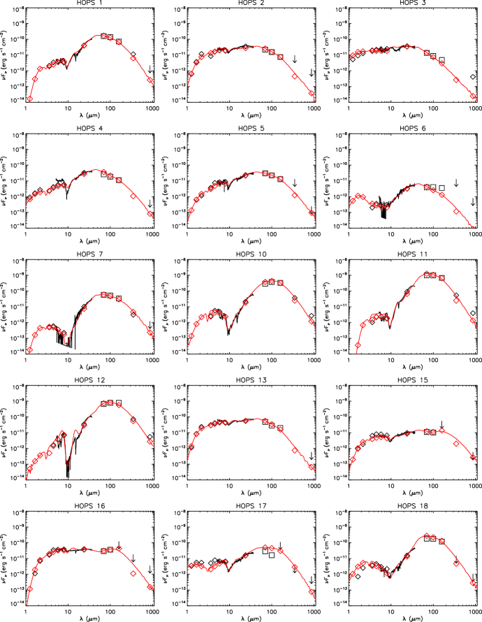
Figure 53: SEDs of the HOPS targets modeled in this work (black; open symbols: photometry, arrows: upper limits, line: IRS spectrum). The best-fit model for each object is shown as a red line, with fluxes taken from a 4″ aperture for $\lambda<8$ $\mu$m, a 5″ aperture for $\lambda=8-37$ $\mu$m, and a 10″ aperture for $\lambda>37$ $\mu$m. The red symbols are the model photometry measured in the same apertures and bandpasses as the data (see Section 4.2 for details).

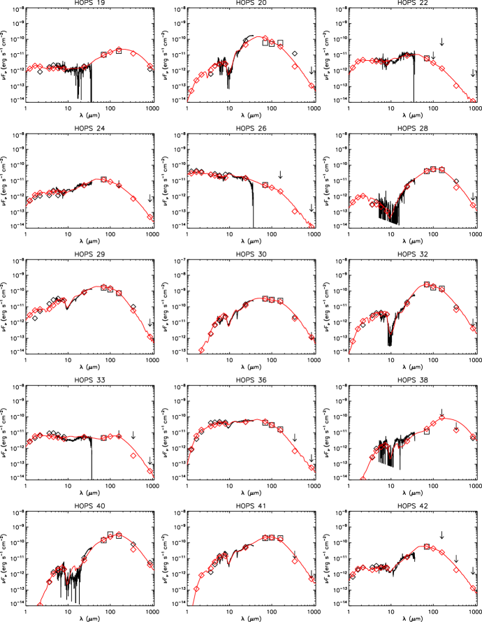
Figure 53: continued.

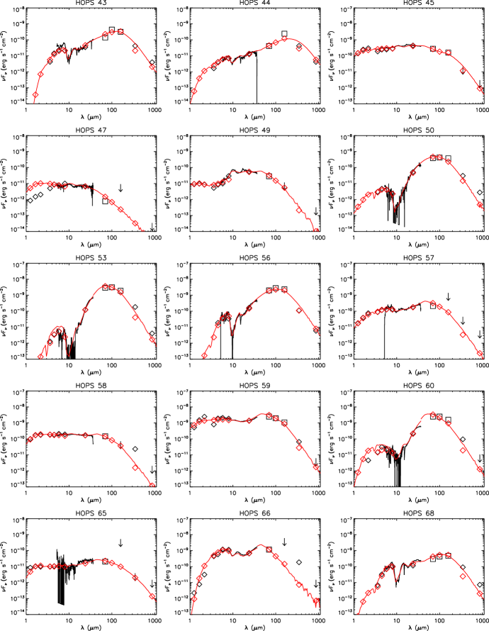
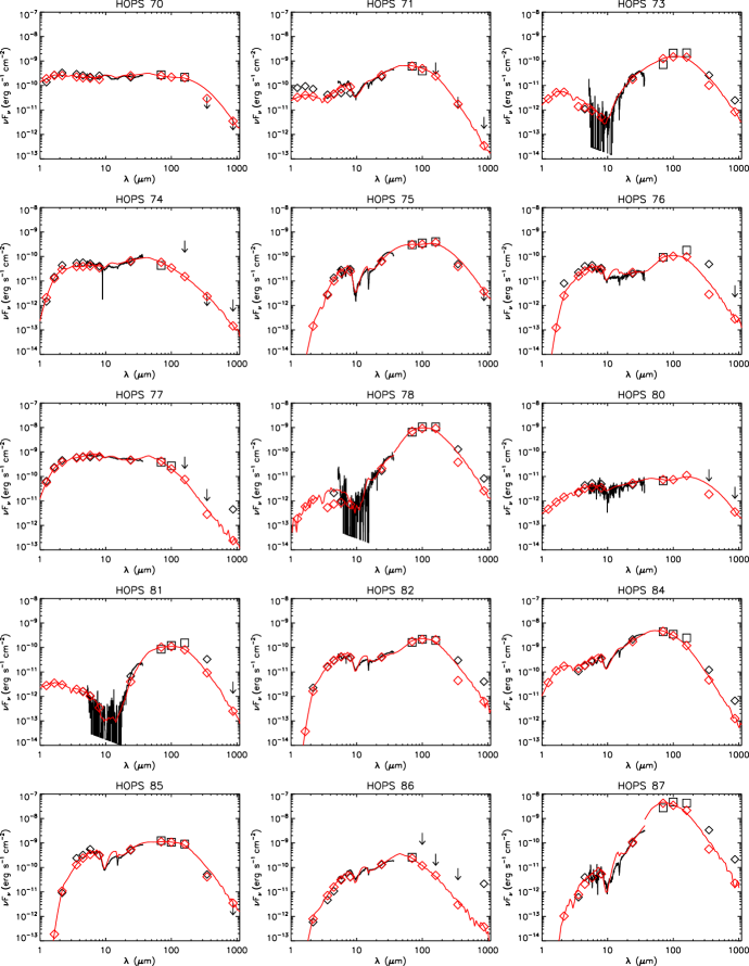
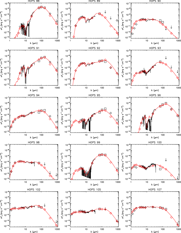
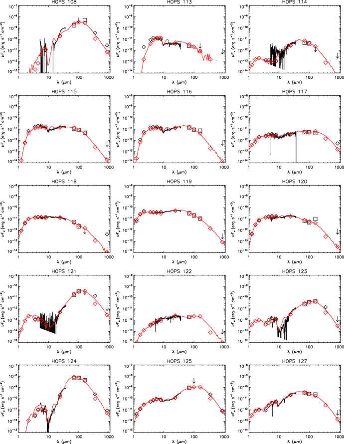
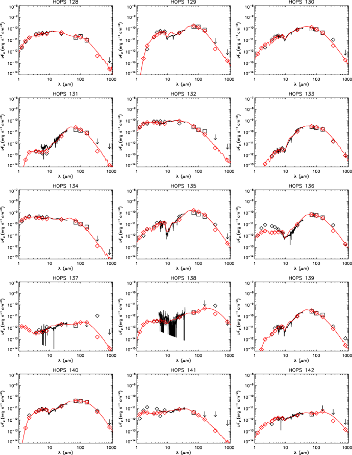
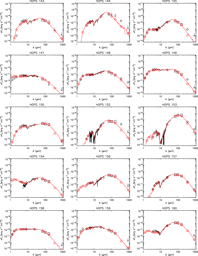
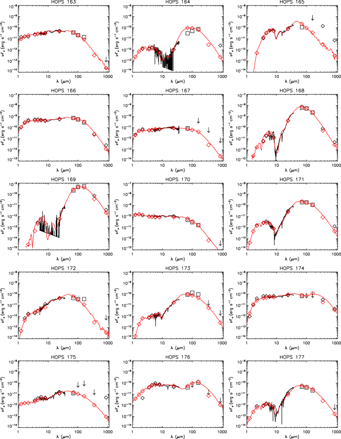
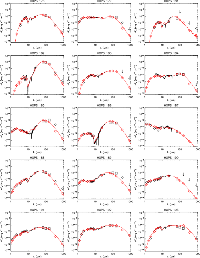
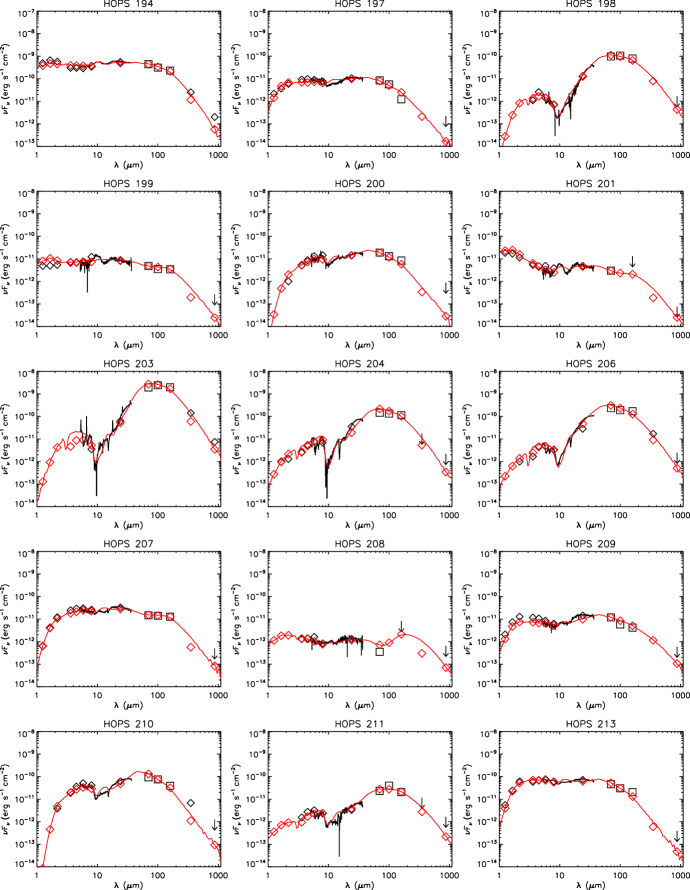
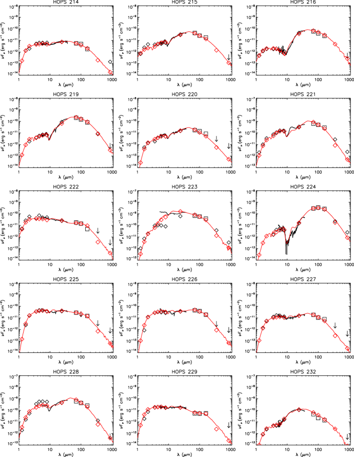
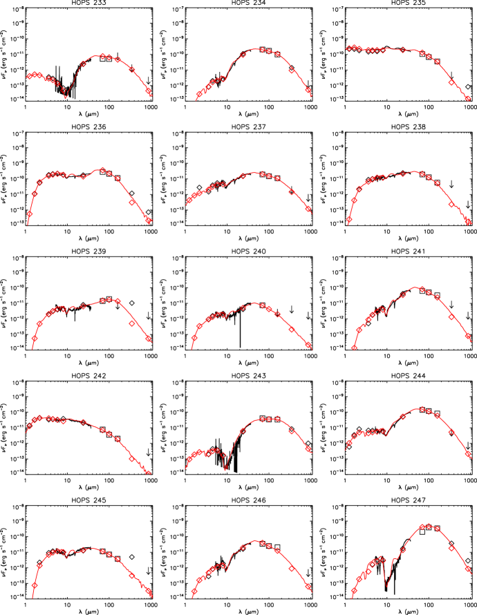
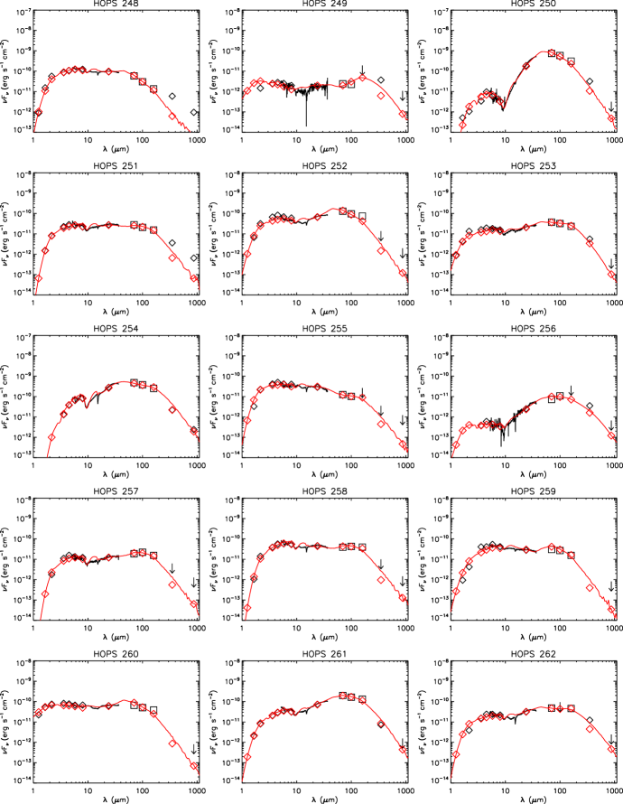
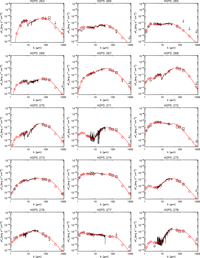
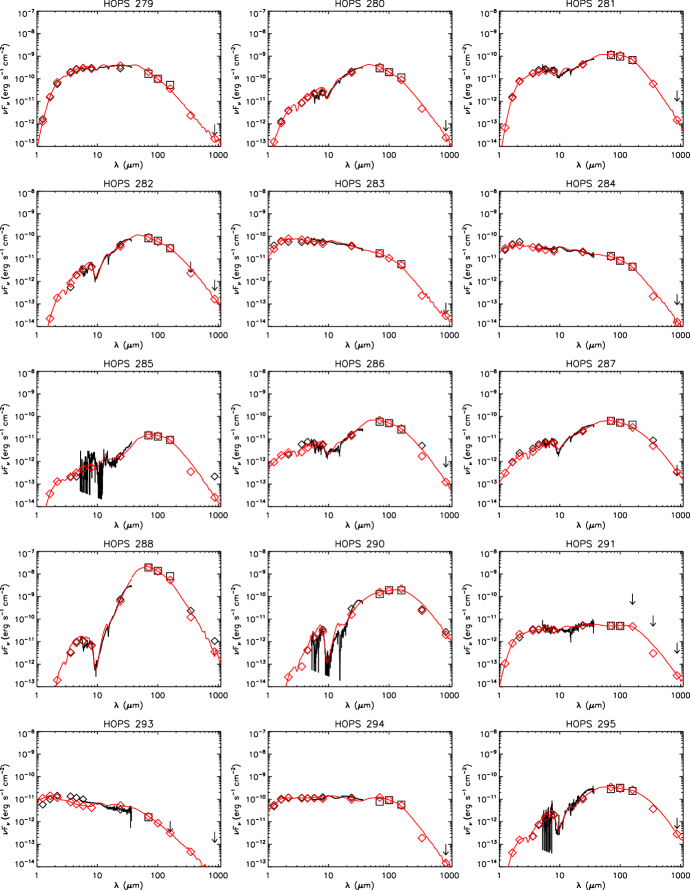
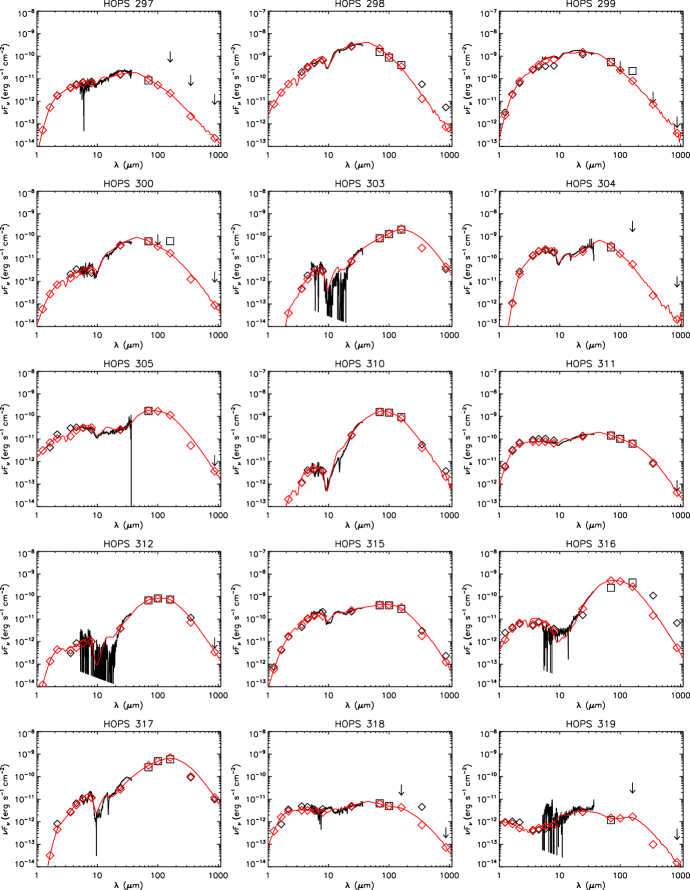
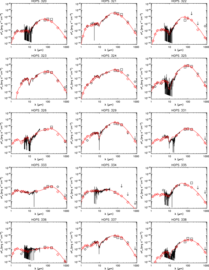
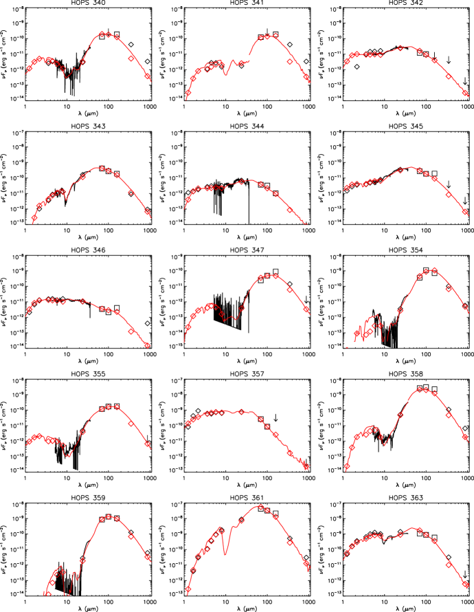
Figure 53: continued.

Figure 53: continued.

Figure 53: continued.

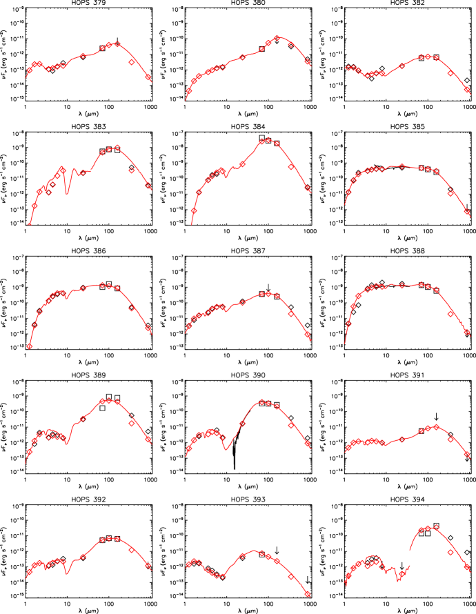
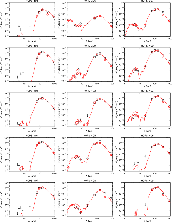
Figure 53: continued.

Figure 53: continued.

Figure 53: continued.

Figure 53: continued.

Figure 53: continued.

Figure 53: continued.

Figure 53: continued.

Figure 53: continued.

Figure 53: continued.

Figure 53: continued.

Figure 53: continued.

Figure 53: continued.

Figure 53: continued.

Figure 53: continued.

Figure 53: continued.

Figure 53: continued.

Figure 53: continued.

Appendix B Spectral Energy Distributions and Variability

The data sets used for the SEDs presented in this work were taken with different instruments and telescopes and are not contemporaneous, yet we know that the majority of protostars are variable at a $\sim$ 20% level (e.g., Morales-Calderón et al., 2011; Billot et al., 2012; Megeath et al., 2012). Therefore, different data sets are snapshots of the emission of the protostar at particular times of its unknown duty cycle of variability. Indeed, in some cases we observe large mismatches between different data sets; an extreme example, the outbursting protostar HOPS 223, was studied by Fischer et al. (2012). Another HOPS protostar that recently experienced an outburst, HOPS 383 (Safron et al., 2015), does not have a mismatched SED, since the photometry used here is representative of the post-outburst SED. In general, variability that is wavelength-dependent or has a long duty cycle is more difficult to determine.

Figure 75: Ratios of photometric fluxes in the IRAC and MIPS bands over those derived from the IRS spectrum. In the left panel, flux ratios at 24 $\mu$m versus those at 5.8 $\mu$m are shown, while in the right panel the 24 $\mu$m flux ratios are plotted versus the 8.0 $\mu$m flux ratios. A ratio of 0 for a certain band means that for that particular object, the IRS spectrum was not available over the wavelength region of that band.

Since 290 of the 330 objects in the HOPS sample that were modeled have an IRS spectrum and measurements with IRAC or MIPS, we compared fluxes measured in the same wave bands, but at different times, to see whether there are discrepancies. We used the Spitzer Science Center’s spitzer_synthphot code to calculate IRAC 5.8 and 8.0 $\mu$m and MIPS 24 $\mu$m synthetic photometry from the IRS fluxes. In Figure B75, we show the flux ratios of IRAC or MIPS photometry and the synthetic photometry using the IRS spectrum for the protostars in our HOPS sample. If there were no mismatches, the flux ratios of IRAC or MIPS and IRS photometry would be close to one. However, we find that they are typically somewhat less than 1; the median ratios at 5.8, 8.0, and 24 $\mu$m are 0.89, 0.95, and 0.83, respectively. For small mismatches, calibration uncertainties are a plausible explanation. In addition, since we are dealing with objects that are not necessarily point sources and often embedded in extended emission, differences in aperture sizes between different measurements (IRAC vs. MIPS vs. IRS) could also account for flux mismatches.

Table 1: Potentially Variable HOPS Targets

Object	Class	[5.8] Ratio	[8.0] Ratio	[24] Ratio
(1)	(2)	(3)	(4)	(5)
HOPS 3	flat	1.681	1.906	1.656
HOPS 7	0	1.121	3.176	1.061
HOPS 11	0	0.444	0.405	0.510
HOPS 12	0	0.553	0.888	0.485
HOPS 19	flat	1.296	1.059	1.648
HOPS 20	I	2.543	2.059	2.329
HOPS 24	I	0.329	0.953	0.824
HOPS 32	0	1.575	1.988	1.041
HOPS 38	0	3.566	2.478	2.468
HOPS 41	I	0.788	0.586	0.495
HOPS 65	I	0.191	1.275	0.969
HOPS 71	I	0.416	0.547	0.825
HOPS 78	0	0.097	$\cdots$	0.664
HOPS 85	flat	1.728	1.445	1.418
HOPS 91	0	0.511	0.446	0.711
HOPS 95	0	2.450	2.106	1.001
HOPS 108	0	$\cdots$	0.867	0.525
HOPS 114	I	0.102	0.132	0.850
HOPS 121	0	$\cdots$	$\cdots$	0.357
HOPS 124	0	0.402	0.601	0.697
HOPS 131	I	0.341	0.270	0.714
HOPS 132	flat	1.717	1.264	0.622
HOPS 138	0	0.354	0.485	0.935
HOPS 141	flat	0.393	1.418	1.086
HOPS 143	I	1.793	1.862	1.039
HOPS 154	I	2.252	1.856	0.814
HOPS 177	I	1.740	2.279	0.863
HOPS 181	I	1.301	1.194	0.492
HOPS 182	0	0.772	0.705	1.390
HOPS 183	flat	0.466	0.502	0.486
HOPS 186	I	1.062	1.999	0.872
HOPS 187	flat	0.321	1.155	0.664
HOPS 203	0	$\cdots$	0.481	0.737
HOPS 206	0	1.106	1.295	0.487
HOPS 222	II	0.496	0.604	0.526
HOPS 223	I	0.070	0.065	0.575
HOPS 228	I	2.098	2.749	0.766
HOPS 239	I	0.682	0.905	1.325
HOPS 270	I	1.729	1.560	0.928
HOPS 271	I	0.948	1.679	1.538
HOPS 272	II	1.660	1.732	1.420
HOPS 278	I	0.651	2.287	2.306
HOPS 290	0	2.198	2.263	1.301
HOPS 297	I	2.083	1.263	0.777
HOPS 299	I	0.454	0.412	0.722
HOPS 305	flat	0.424	0.423	0.422
HOPS 316	0	2.279	1.662	0.432
HOPS 319	I	0.218	0.520	0.796
HOPS 321	I	0.769	0.518	0.662
HOPS 322	I	0.128	0.494	0.680
HOPS 338	0	1.552	1.683	1.376
HOPS 340	0	1.192	0.863	0.522
HOPS 358	0	$\cdots$	$\cdots$	0.514
HOPS 359	0	$\cdots$	$\cdots$	0.517
HOPS 363	flat	1.169	1.242	1.616
HOPS 388	flat	1.058	1.896	1.479

Note. — Column (1) lists the HOPS number of the object, column (2) the class based on SED classification, column (3) the ratio of the IRAC 5.8 µm flux and the IRS flux over the IRAC 5.8 µm band, columns (4) and (5) the ratio of photometric and IRS flux for the IRAC 8.0 µm and MIPS 24 µm band, respectively.

To identify outliers, in Table B1, we list those flux ratios that lie in the lower or upper 5% of values. They represent a conservative list of potentially variable sources in our sample. Of the 290 objects for which we calculated flux ratios, 5 have flux mismatches larger than a factor of 2 between IRS and both IRAC bands at 5.8 and 8.0 $\mu$m. Three objects have similarly large mismatches between IRS and MIPS. The overlap between these two samples contains two objects, HOPS 20 and 38 (the other objects are HOPS 95, 228, 278, and 290). For most of these objects, the large mismatches can be attributed to noisy IRS spectra, especially in the 5-8 $\mu$m region, making the comparison between IRAC and IRS less reliable. Eight objects have IRAC-IRS mismatches smaller than a factor 0.5; one of these objects and seven different objects have such small mismatches between MIPS and IRS (see Table B1). Slightly over one-third of these objects have noisy IRS spectra. Of the 21 objects that have either large ($>$ factor of 2) or small ($<$ factor of 0.5) mismatches, 9 are Class 0 protostars, 10 are Class I protostars, and 2 are flat-spectrum sources. In cases where the IRS flux is too high relative to the MIPS 24 $\mu$m photometry, the mismatch could be due to more extended emission or flux from a nearby companion being included in the IRS measurement (SL and LL slit widths of 3$\farcs$6 and 10$\farcs$5, respectively, versus the typical FWHM of the MIPS 24 $\mu$m PSF of $\sim$ 6″).

For a few sources, the discrepancies between IRS fluxes and IRAC or MIPS can be attributed to the scaling factors applied to different parts of the IRS spectrum. As mentioned in section 3, we typically scaled the SL spectrum to match the flux of the LL spectrum at 14 $\mu$m, given that the latter has a larger slit width. However, in the case of HOPS 38, where the IRAC 5.8 and 8.0 $\mu$m and the MIPS 24 $\mu$m fluxes are about a factor of 2.5-3.5 higher than the IRS fluxes, the LL spectrum was scaled by 0.4 to match the SL flux at 14 $\mu$m. Given the IRAC and MIPS measurements, it would have been more appropriate to scale the SL spectrum up. For HOPS 124, the SL spectrum was scaled by 2.5; if instead the LL spectrum had been scaled down, the discrepancies between IRS and IRAC and MIPS would be less than 50%.

Overall, in cases where the IRS spectrum has sufficient signal-to-noise ratio and its fluxes seem lower than the photometric measurements or the discrepancies in IRAC-IRS and MIPS-IRS fluxes are quite different, intrinsic source variability could be a likely explanation. Among the sample shown in Table B1, this would apply to HOPS 24, 71, 131, 132, 141, 143, 154, 187, 206, 223, 228, 299, 363, and 388. HOPS 223 is indeed variable (see Fischer et al., 2012), but the other objects still require confirmation. Thus, about 5% of the 290 protostars in our HOPS sample that have IRS, IRAC, and MIPS data may reveal variability to some degree. These objects are prime candidates for follow-up observations regarding their variability.

Appendix C Model Parameter Ranges and Degeneracies

In section 6.4 we discussed how modes can be used to assess how well model parameters are constrained. Here we analyze the spread of mode values for individual HOPS targets. In Figure Set C1 (see Fig. C76 for an example) we show the difference between the modes and the best-fit values of the major model parameters ($i,L_{tot},\rho_{1000},\theta,R_{disk},A_{V}$) for all modeled HOPS targets. As in section 6.4, we use models in certain $\Delta R$ bins, starting at a range of 0.5 from the best-fit $R$ up to a range of 2.0 from the best-fit $R$. For parameters with discrete values, such as the inclination and cavity opening angles, we plot the difference between the indices of modes and best-fit values. For example, if the best-fit inclination angle has a value of 41° and the mode a value of 57°, the difference in indices would be 2 (since the discrete values in our model grid are 18°, 32°, 41°, 50°, 57°, etc.). Similarly, if the best-fit cavity opening angle is 5° but the mode is 45°, the difference in indices would be 4. For the total luminosity and foreground extinction, we plotted instead the difference between the parameter values of the best fit and the modes.

Objects that are not particularly well fit by their best-fit model from the grid often have modes that are quite different from the best-fit value once $\Delta R$ reaches 2. For example, for HOPS 181, whose best-fit model has $R$=5.16, the mode of the inclination angle for models within $\Delta R$=0.5 (i.e., models with $R<5.66$) is the same as the best-fit value, but then the difference increases as $\Delta R$ becomes larger. For $\Delta R$=2.0, the mode is seven discrete values away from the best fit ($i=$18° for the mode, 76° for the best fit). Several other model parameters are also not well constrained. There are also objects that have a relatively good fit, but a larger spread in certain parameters. An example is HOPS 70, whose best-fit model has an $R$ value of 2.33; its total luminosity and inclination angle are very well constrained, while its reference envelope density is quite uncertain.

Certain protostars are sufficiently well constrained by the available data and well fit by our grid of models that their parameters do not change much from $\Delta R$=0.5 to $\Delta R$=2.0. For example, the modes of the inclination angle of HOPS 1 are the same as the best-fit value even for all models within $\Delta R$=2, and the other model parameters show a small spread. There are 37 protostars with small differences between their best-fit values and modes for models within $\Delta R$=2 ($<$ factor of two for $\rho_{1000}$ and $L_{tot}$, $<$ 50 AU for the disk radius, $<$ 10° for the cavity opening angle, $<$ 30% difference in inclination angle). These protostars are well characterized by our model fits. The mean and median $R$ values for their best-fit models are 3.48 and 3.17, respectively. This validates our estimate of $R\sim$ 4 as the boundary between a reliable and a less reliable fit.

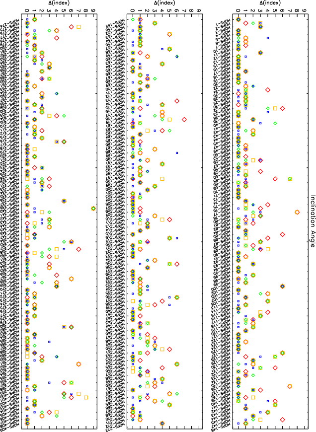
Figure 76: For all modeled HOPS targets (see name on x axis), difference between the index of the best-fit inclination angle and the index of the mode of the inclination angle for models that lie within a difference of 0.5 (small blue squares), 1.0 (small green diamonds), 1.5 (yellow larger squares), and 2.0 (red larger diamonds) of the best-fit $R$. The remaining plots for the other five model parameters are available in Figure Set C1.

Fig. SetC1. Figure set showing the differences between modes and best-fit parameter values of six model parameters for all modeled HOPS targets.

Part of the parameter uncertainties can be attributed to degeneracies between model parameters. To illustrate some of these degeneracies, in Figure Set C2 (see Fig. C77 for an example) we show contour plots of $R$ values for sets of two model parameters each (we plot the lowest $R$ value of models with these two parameter values) resulting from the model fits of HOPS 24, HOPS 107, and HOPS 149. The plots for HOPS 24 show that the inclination angle is somewhat degenerate with the envelope density, with higher inclination angles being accommodated by lower $\rho_{1000}$ values (Fig. C77). A similar situation applies to the disk radius, with larger disk radii requiring higher envelope densities. The inclination angle and the cavity opening angle are degenerate, too; for higher inclination angles the cavity is larger. The $R$ contour plots for HOPS 107 suggest that a certain range of inclination angles and reference densities can fit the SED, while the disk radius and cavity opening angles are not well constrained. However, the plots clearly show that high-density, high-inclination models fit very poorly. Finally, we can deduce from the $R$ contour plots for HOPS 149 that also here certain parameter values can be excluded; lower inclination angles and reference densities in the 10^-18–10^-19 g cm^-3 range yield the best fits, with larger densities accompanied by larger disk radii and larger cavity opening angles.

Figure 77: $R$ contour plot for the models that fit HOPS 24. For each combination of inclination angle and reference density, the lowest $R$ values of models with these two parameter values are shown. The remaining $R$ contour plots are available in Figure Set C2.

Fig. SetC2. Figure set showing ten examples of $R$ contour plots.

Appendix D Notes on HOPS Targets

D.1 HOPS Targets Discovered with Herschel

Table 1: New Protostars from Stutz et al. (2013) and Tobin et al. (2015)

HOPS Identifier	Original ID	R.A.	Dec.
		[$\arcdeg$]	[$\arcdeg$]
(1)	(2)	(3)	(4)
HOPS 394	019003	83.8497	-5.1315
HOPS 395	026011	84.8208	-7.4074
HOPS 396	029003	84.8048	-7.2199
HOPS 397	061012	85.7036	-8.2696
HOPS 398	082005	85.3725	-2.3547
HOPS 399	082012	85.3539	-2.3024
HOPS 400	090003	85.6885	-1.2706
HOPS 401	091015	86.5319	-0.2058
HOPS 402	091016	86.5415	-0.2047
HOPS 403	093005	86.6156	-0.0149
HOPS 404	097002	87.0323	0.5641
HOPS 405	119019	85.2436	-8.0934
HOPS 406	300001	86.9307	0.6396
HOPS 407	302002	86.6177	0.3242
HOPS 408	313006	84.8781	-7.3998
HOPS 409	135003	83.8392	-5.2215

Note. — Column (1) lists the HOPS number of the object, column (2) the identifier of the source from Stutz et al. (2013) and Tobin et al. (2015), and columns (3) and (4) its J2000 coordinates in degrees.

D.2 HOPS Objects not Included in the Modeling Sample

D.2.1 Young Stellar Objects

Among our HOPS sample, there are 41 targets that are likely YSOs, but they lack PACS measurements at 70 and 160 $\mu$m and were therefore not included in the modeling sample. There are four additional targets with HOPS numbers that were not modeled; they are HOPS 109, 111, 212, and 362, and they are duplicates of HOPS 40, 60, 211, and 169, respectively. Table D2 lists the 41 likely YSOs in the HOPS catalog that were not part of the modeling sample; their SEDs are shown in Figure D78. Among them, 17 were not observed by PACS at 70 $\mu$m, while 24 were observed, but not detected at 70 $\mu$m. The majority of these targets are Class I protostars or flat-spectrum sources; only one is a Class 0 protostar, and five are Class II pre-main-sequence stars.

Most of these YSOs have very faint fluxes in the near- to mid-IR. They could be deeply embedded protostars, like HOPS 307, or just very low-mass protostars with weak envelope emission. Objects with little excess emission out to about 8 $\mu$m, a 10 $\mu$m silicate emission feature, and a more or less steeply rising SED beyond 12 $\mu$m are likely transitional disks (see Kim et al., 2013); good examples are HOPS 51 and 54. It is possible that some of the YSOs in this sample are actually extragalactic contaminants, in particular objects with flat SEDs (see more about this subset of our HOPS sample in the next subsection).

Table 2: YSOs in the HOPS Sample with No PACS Data

Object	R.A.	Dec.	Class	$L_{bol}$	$T_{bol}$	$n_{4.5-24}$	PACS Flag
	[$\arcdeg$]	[$\arcdeg$]		[$L_{\odot}$]	[K]
(1)	(2)	(3)	(4)	(5)	(6)	(7)	(8)
HOPS 0	88.6171	1.6264	I	0.011	652.2	0.514	-1
HOPS 8	83.8880	-5.9851	I	0.013	329.8	0.419	0
HOPS 9	83.9550	-5.9843	I	0.006	281.5	0.858	-1
HOPS 14	84.0799	-5.9251	flat	0.042	464.0	0.246	0
HOPS 23	84.0745	-5.7818	I	0.012	346.8	0.539	0
HOPS 25	83.8443	-5.7415	flat	0.045	646.6	0.165	0
HOPS 31	83.8219	-5.6741	flat	0.024	634.7	0.304	0
HOPS 34	83.7954	-5.6585	I	0.013	235.5	0.762	0
HOPS 35	83.8331	-5.6503	I	0.044	305.2	0.884	0
HOPS 37	83.6986	-5.6237	flat	0.016	913.4	0.230	0
HOPS 51	83.8160	-5.5015	II	0.518	130.2	$\cdots$	0
HOPS 52	83.8180	-5.4924	flat	0.641	610.8	-0.163	0
HOPS 54	83.3437	-5.3841	II	0.097	1879.3	-0.37	-1
HOPS 62	83.8524	-5.1916	flat	0.660	1154.1	0.043	0
HOPS 63	83.8538	-5.1671	flat	0.516	544.5	0.004	0
HOPS 64	83.8625	-5.1650	I	15.347	29.7	0.503	0
HOPS 69	83.8551	-5.1400	flat	2.778	31.3	-0.189	0
HOPS 79	83.8662	-5.0934	flat	0.086	666.2	-0.137	0
HOPS 103	83.5508	-4.8353	flat	0.142	1484.3	-0.032	0
HOPS 104	83.7782	-4.8338	I	0.044	337.3	0.837	0
HOPS 110	84.0093	-5.0472	I	0.014	244.0	$\cdots$	-1
HOPS 126	85.0408	-7.1650	flat	0.132	1865.3	-0.136	-1
HOPS 151	84.6787	-6.9447	II	0.061	799.4	-0.505	0
HOPS 155	84.3160	-7.2972	flat	0.013	393.8	0.133	-1
HOPS 162	84.1291	-6.8780	II	0.015	909.9	0.352	-1
HOPS 180	84.2475	-6.1710	II	0.011	1493.5	0.578	-1
HOPS 195	84.0002	-6.1206	flat	0.032	659.7	0.399	0
HOPS 217	85.7965	-8.4056	I	0.008	323.8	0.773	-1
HOPS 230	85.6283	-8.1515	flat	0.267	1260.2	-0.104	-1
HOPS 231	85.1189	-8.5486	flat	0.024	386.0	-0.239	-1
HOPS 269	85.3625	-7.7094	flat	0.025	230.2	0.023	-1
HOPS 289	84.9865	-7.5017	I	0.095	331.1	0.868	0
HOPS 296	85.3215	-2.3021	I	0.022	326.0	0.931	0
HOPS 302	85.0934	-2.2610	flat	0.383	1367.2	-0.032	-1
HOPS 307	85.3077	-1.7844	0	0.748	57.1	1.506	-1
HOPS 314	86.6505	-0.3414	I	0.015	276.2	1.112	-1
HOPS 327	86.6139	0.1477	flat	0.020	991.0	0.145	-1
HOPS 328	86.5561	0.1759	I	0.012	326.3	0.868	-1
HOPS 330	86.7140	0.3298	flat	0.121	385.2	0.285	0
HOPS 332	86.8821	0.3391	flat	0.249	145.5	0.045	0
HOPS 360	86.8629	0.3425	I	1.017	43.2	$\cdots$	0

Note. — Column (1) lists the HOPS number of the object, columns (2) and (3) its J2000 coordinates in degrees, column (4) the type based on SED classification, column (5) the bolometric luminosity, column (6) the bolometric temperature, column (7) the 4.5-24 $\mu$m SED slope, and column (8) a flag identifying whether the object was not observed by PACS (flag value of -1), or not detected by PACS at 70 $\mu$m (flag value of 0)

Figure 78: SEDs of the HOPS targets not modeled in this work that are likely YSOs (open symbols: photometry, line: IRS spectrum).

Figure 78: continued.

Figure 78: continued.

D.2.2 Contaminants

Our HOPS sample contains 29 targets that turned out to be likely extragalactic contaminants. These objects are listed in Table D3, and their SEDs are shown in Figure D81. Most galaxies were identified based on the presence of PAH features or emission lines in their IRS spectra (in particular, the 5–15 $\mu$m region), the absence of a silicate absorption feature at 10 $\mu$m, and an overall flat or slightly rising mid-infrared continuum. Clear examples are HOPS 21, 27, 46, 48, 55, 61, 72, 106, 161, and 301.

Two objects, HOPS 202 and HOPS 205, have a tentative 10 $\mu$m silicate emission feature and a steep rise of their SED beyond 12 $\mu$m, but also PAH emission features in their IRS spectrum; they could be transitional disks and not galaxies.

In some cases, e.g., HOPS 308, targets classified as extragalactic contaminants are very faint in the near- to mid-infrared; instead of galaxies, they could be very low-mass or deeply embedded protostars.

The mid-IR SED of HOPS 339 is mostly flat but displays a sharp 10 $\mu$m absorption feature; based on the SED alone, it would not necessarily be classified as a galaxy, but high-resolution near-IR HST images resolve its extended emission and reveal a spiral galaxy (J. Booker et al. 2016, in preparation).

Finally, HOPS 349, 350, 352, 353, 356, and 381 have poorly sampled SEDs (just one or two flux measurements), so their nature is quite uncertain. We list their coordinates in Table D4.

Table 3: Likely Extragalactic Contaminants in the HOPS Sample

Object	R.A.	Dec.	$L_{bol}$	$T_{bol}$	$n_{4.5-24}$
	[$\arcdeg$]	[$\arcdeg$]	[$L_{\odot}$]	[K]
(1)	(2)	(3)	(4)	(5)	(6)
HOPS 21	84.0421	-5.8356	0.074	584.5	0.824
HOPS 27	84.0905	-5.6995	0.102	118.2	0.458
HOPS 39	84.0934	-5.6069	0.100	159.4	1.010
HOPS 46	83.6758	-5.5509	0.141	1081.9	-0.083
HOPS 48	83.7773	-5.5477	0.608	611.0	0.252
HOPS 55	83.4754	-5.3638	0.316	101.5	1.732
HOPS 61	83.3579	-5.2007	0.045	721.4	-0.031
HOPS 67	83.8445	-5.1428	0.044	278.7	0.900
HOPS 72	83.8571	-5.1296	0.545	693.0	0.068
HOPS 83	83.9822	-5.0771	0.131	293.9	-0.119
HOPS 97	83.8704	-4.9608	0.190	403.8	0.125
HOPS 101	83.7843	-4.9027	3.355	481.2	-0.207
HOPS 106	84.0518	-4.7544	0.016	359.7	0.943
HOPS 112	85.1833	-7.3786	0.014	390.2	0.093
HOPS 146	84.6840	-7.0112	0.053	519.7	-0.178
HOPS 161	84.1448	-7.1871	0.062	179.1	0.458
HOPS 196	83.8371	-6.3062	0.065	165.5	-0.042
HOPS 202	83.4330	-6.2295	0.018	736.3	0.534
HOPS 205	85.7620	-8.7971	0.067	427.8	0.549
HOPS 218	85.7912	-8.2232	0.007	332.5	0.653
HOPS 292	84.4787	-7.6890	0.068	280.5	0.421
HOPS 301	85.4366	-2.2654	2.955	518.8	0.271
HOPS 306	85.7630	-1.8013	0.038	310.8	0.060
HOPS 308	85.8082	-1.7195	0.042	156.0	0.791
HOPS 309	85.6973	-1.4131	0.041	111.9	-0.168
HOPS 313	85.2532	-1.1529	0.030	154.1	1.039
HOPS 339	86.4733	0.4243	0.128	398.3	0.246
HOPS 348	86.7511	0.3438	0.286	84.0	$\cdots$
HOPS 351	83.8809	-5.0797	0.016	217.1	$\cdots$

Note. — Column (1) lists the HOPS number of the object, columns (2) and (3) its J2000 coordinates in degrees, column (4) the bolometric luminosity, column (5) the bolometric temperature, and column (6) the 4.5-24 $\mu$m SED slope.

Table 4: Targets in the HOPS Sample with Uncertain Nature

Object	R.A.	Dec.
(1)	(2)	(3)
HOPS 349	83.8592	-5.1426
HOPS 350	83.8758	-5.1386
HOPS 352	83.8617	-5.0675
HOPS 353	88.5556	1.7175
HOPS 356	85.5341	-1.4438
HOPS 381	83.7816	-5.6986

Note. — Column (1) lists the HOPS number of the object, columns (2) and (3) its J2000 coordinates in degrees.

Figure 81: SEDs of the HOPS targets not modeled in this work that are likely extragalactic contaminants (open symbols: photometry, line: IRS spectrum).

Figure 81: continued.

References

- Adams & Shu (1986) Adams, F. C., & Shu, F. H. 1986, ApJ, 308, 836
- Adams, Lada, & Shu (1987) Adams, F. C., Lada, Ch. J., & Shu, F. H. 1987, ApJ, 312, 788
- Adams et al. (2012) Adams, J. D., Herter, T. L., Osorio, M., et al. 2012, ApJL, 749, L24
- Ali et al. (2010) Ali, B., Tobin, J. J., Fischer, W. J., et al. 2010, A&A, 518, L119
- André et al. (1993) André, P., Ward-Thompson, D., & Barsony, M. 1993, ApJ, 406, 122
- André & Montmerle (1994) André, P., & Montmerle, T. 1994, ApJ, 420, 837
- André et al. (2010) André, P., Men’shchikov, A., Bontemps, S., et al. 2010, A&A, 518, L102
- Arce & Sargent (2006) Arce, H. G., & Sargent, A. I. 2006, ApJ, 646, 1070
- Billot et al. (2012) Billot, N., Morales-Calderón, M., Stauffer, J. R., et al. 2012, ApJL, 753, L35
- Boogert et al. (2008) Boogert, A. C. A., Pontoppidan, K. M., Knez, C., et al. 2008, ApJ, 678, 985
- Calvet et al. (1994) Calvet, N., Hartmann, L., Kenyon, S. J., & Whitney, B. A. 1994, ApJ, 434, 330
- Caratti o Garatti (2011) Caratti o Garatti, A., Garcia Lopez, R., Scholz, A., et al. 2011, A&A, 526, L1
- Cassen & Moosman (1981) Cassen, P., & Moosman, A. 1981, Icarus, 48, 353
- Chen et al. (1995) Chen, H., Myers, P. C., Ladd, E. F., & Wood, D. O. S. 1995, ApJ, 445, 377
- Cody et al. (2014) Cody, A. M., Stauffer, J., Baglin, A., et al. 2014, AJ, 147, 82
- Cohen et al. (2003) Cohen, M., Wheaton, W. A., & Megeath, S. T. 2003, AJ, 126, 1090
- Crapsi et al. (2008) Crapsi, A., van Dishoeck, E. F., Hogerheijde, M. R., et al. 2008, A&A, 486, 245
- di Francesco et al. (2007) di Francesco, J., Evans, N. J., II, Caselli, P., et al. 2007, in Protostars & Planets V, Reipurth B., Jewitt D., Keil K. (eds.), Univ. Arizona, Tucson, p. 17
- Draine (2003) Draine, B. T. 2003, ARA&A, 41,241
- Dunham et al. (2008) Dunham, M. M., Crapsi, A., Evans, N. J., II, et al. 2008, ApJS, 179, 249
- Dunham et al. (2010) Dunham, M. M., Evans, N. J., II, Terebey, S., et al. 2010, ApJ, 710, 470
- Dunham & Vorobyov (2012) Dunham, M. M., & Vorobyov, E. I. 2012, ApJ, 747, 52
- Dunham et al. (2013) Dunham, M. M., Arce, H. G., Allen, L. E., et al. 2013, AJ, 145, 94
- Dunham et al. (2014) Dunham, M. M., Stutz, A. M., Allen, L. E., et al. 2014, in Protostars & Planets VI, Beuther H., Klessen R. S., Dullemond C. P., Henning T. (eds.), Univ. Arizona, Tucson, p. 195
- Dunham et al. (2015) Dunham, M. M., Allen, L. E., Evans, N. J., II, et al. 2015, ApJS, 220, 11
- Engelbracht et al. (2007) Engelbracht, C. W., Blaylock, M., Su, K. Y. L., et al. 2007, PASP, 119, 994
- Enoch et al. (2009) Enoch, M., Evans, N. J., II, Sargent, A. I., & Glenn, J. 2009, ApJ, 692, 973
- Espaillat et al. (2014) Espaillat, C., Muzerolle, J., Najita, J., et al. 2014, in Protostars & Planets VI, Beuther H., Klessen R. S., Dullemond C. P., Henning T (eds.), Univ. Arizona, Tucson, p. 497
- Evans et al. (2001) Evans, N. J., II, Rawlings, J. M. C., Shirley, Y. L., & Mundy, L. G. 2001, ApJ, 557, 193
- Evans et al. (2009) Evans, N. J., II, Dunham, M. M., Jørgensen, J. K., et al. 2009, ApJS, 181, 321
- Fazio et al. (2004) Fazio, G. G., Hora, J. L., Allen, L. E., et al. 2004, ApJS,154, 10
- Fischer et al. (2010) Fischer, W. J., Megeath, S. T., Ali, B., et al. 2010, A&A, 518, L122
- Fischer et al. (2012) Fischer, W. J., Megeath, S. T., Tobin, J. J., et al. 2012, ApJ, 756, 99
- Fischer et al. (2013) Fischer, W. J., Megeath, S. T., Stutz, A. M., et al. 2013, AN, 334, 53
- Fischer et al. (2014) Fischer, W. J., Megeath, S. T., Tobin, J. J., et al. 2014, ApJ, 781, 123
- Furlan et al. (2008) Furlan, E., McClure, M., Calvet, N., et al. 2008, ApJS, 176, 184
- Furlan et al. (2014) Furlan, E., Megeath, S. T., Osorio, M., et al. 2014, ApJ, 786, 26
- Greene et al. (1994) Greene, T. P., Wilking, B. A., André, P., et al. 1994, ApJ, 434, 614
- Günther et al. (2014) Günther, H. M., Cody, A. M., Covey, K. R., et al. 2014, AJ, 148, 122
- Hartmann et al. (1996) Hartmann, L., Calvet, N., & Boss, A., 1996, ApJ, 464, 387
- Heiderman & Evans (2015) Heiderman, A., & Evans, N. J., II 2015, ApJ, 806, 231
- Houck et al. (2004) Houck, J. R., Roellig, T. L., van Cleve, J., et al. 2004, ApJS, 154, 18
- Kenyon et al. (1990) Kenyon, S. J., Hartmann, L. W., Strom, K. M., & Strom, S. E. 1990, AJ, 99, 869
- Kenyon et al. (1993) Kenyon, S. J., Calvet, N., & Hartmann, L. 1993, ApJ, 414, 676
- Kim et al. (2008) Kim, M. K., Hirota, T., Honma, M., et al. 2008, PASJ, 60, 991
- Kim et al. (2013) Kim, K. H., Watson, D. M., Manoj, P., et al. 2013, ApJ, 769, 149
- Kim et al. (2016) Kim, K. H., Watson, D. M., Manoj, P., et al. 2016, ApJS, submitted
- Kounkel et al. (2016) Kounkel, M., Megeath, S. T., Poteet, C. A., et al. 2016, ApJ, in press, arXiv:1602.07635
- Kryukova et al. (2012) Kryukova, E., Megeath, S. T., Gutermuth, R. A., et al. 2012, AJ, 144, 31
- Kryukova et al. (2014) Kryukova, E., Megeath, S. T., Hora, J. L., et al. 2014, AJ, 148, 11
- Lada (1987) Lada, Ch. J. 1987, in Star Forming Regions, proceedings of the IAU Symposium No. 115, ed. M. Peimbert & J. Jugaku, Dordrecht:Reidel, 1
- Launhardt et al. (2013) Launhardt, R., Stutz, A. M., Schmiedeke, A., et al. 2013, A&A, 551, A98
- Lim & Takakuwa (2006) Lim, J., & Takakuwa, S. 2006, ApJ, 653, 425
- Manoj et al. (2013) Manoj, P., Watson, D. M., Neufeld, D. A., et al. 2013, ApJ, 763, 83
- Mathis et al. (1983) Mathis, J. S., Mezger, P. G., & Panagia, N. 1983, A&A, 128, 212
- Mathis (1990) Mathis, J. S. 1990, ARA&A, 28, 37
- Maury et al. (2011) Maury, A. J., André, P., Men’shchikov, A., et al. 2011, A&A, 535, A77
- McClure (2009) McClure, M. 2009, ApJL, 693, L81
- Megeath et al. (2012) Megeath, S. T., Gutermuth, R., Muzerolle, J., et al. 2012, AJ, 144, 192
- Menten et al. (2007) Menten, K. M., Reid, M. J., Forbrich, J., & Brunthaler, A. 2007, A&A, 474, 515
- Morales-Calderón et al. (2011) Morales-Calderón, M., Stauffer, J. R., Hillenbrand, L. A., et al. 2011, ApJ, 733, 50
- Myers & Ladd (1993) Myers, P. C., & Ladd, E. F. 1993, ApJL, 413, L47
- Offner & McKee (2011) Offner, S. S. R., & McKee, C. F. 2011, ApJ, 736, 53
- Ormel et al. (2011) Ormel, C. W., Min, M., Tielens, A. G. G. M., Dominik, C., & Paszun, D. 2011, A&A, 532, A43
- Ossenkopf & Henning (1994) Ossenkopf, V., & Henning, T. 1994, A&A, 291, 943
- Pilbratt et al. (2010) Pilbratt, G. L., Riedinger, J. R., Passvogel, T., et al. 2010, A&A, 518, L1
- Pillitteri et al. (2013) Pillitteri, I., Wolk, S. J., Megeath, S. T., et al. 2013, ApJ, 768, 99
- Poglitsch et al. (2010) Poglitsch, A., Waelkens, C., Geis, N., et al. 2010, A&A, 518, L2
- Pontoppidan et al. (2008) Pontoppidan, K. M., Boogert, A. C. A., Fraser, H. J., et al. 2008, ApJ, 678, 1005
- Poppenhaeger et al. (2015) Poppenhaeger, K., Cody, A. M., Covey, K. R. 2015, AJ, 150, 118
- Poteet et al. (2011) Poteet, C. A., Megeath, S. T., Watson, D. M., et al. 2011, ApJL, 733, L32
- Reach et al. (2005) Reach, W. T., Megeath, S. T., Cohen, M., et al. 2005, PASP, 117, 978
- Rebull et al. (2014) Rebull, L. M., Cody, A. M., Covey, K. R., et al. 2014, AJ, 148, 92
- Rebull et al. (2015) Rebull, L. M., Stauffer, J. R., Cody, A. M., et al. 2015, AJ, 150, 175
- Rieke et al. (2004) Rieke, G. H., Young, E. T., Engelbracht, C. W., et al. 2004, ApJS, 154, 25
- Robitaille et al. (2006) Robitaille, T. P., Whitney, B. A., Indebetouw, R., et al. 2006, ApJS, 167, 256
- Rodríguez et al. (1998) Rodríguez, L. F., D’Alessio, P., Wilner, D. J., et al. 1998, Nature, 395, 355
- Sadavoy et al. (2014) Sadavoy, S. I., Di Francesco, J., André, P., et al. 2014, ApJL, 787, L18
- Safron et al. (2015) Safron, E. J., Fischer, W. J., Megeath, S. T., et al. 2015, ApJL, 800, L5
- Shirley et al. (2002) Shirley, Y. L., Evans, N. J., II, & Rawlings, J. M. C. 2002, ApJ, 575, 337
- Siringo et al. (2010) Siringo, G., Kreysa, E., De Breuck, C., et al. 2010, The Messenger, 139, 20
- Siringo et al. (2009) Siringo, G., Kreysa, E., Kovács, A., et al. 2009, A&A, 497, 945
- Skrutskie et al. (2006) Skrutskie, M. F., Cutri, R. M., Stiening, R., et al. 2006, AJ, 131, 1163
- Stanke et al. (2010) Stanke, T., Stutz, A. M., Tobin, J. J., et al. 2010, A&A, 518, L94
- Stutz et al. (2010) Stutz, A. M., Launhardt, R., Linz, H., et al. 2010, A&A, 518 L87
- Stutz et al. (2013) Stutz, A. M., Tobin, J. J., Stanke, T., et al. 2013, ApJ, 767, 36
- Stutz & Kainulainen (2015) Stutz, A. M., & Kainulainen 2015, A&A, 577, L6
- Terebey et al. (1984) Terebey, S., Shu, F. H., & Cassen, P. 1984, ApJ, 286, 529
- Tobin et al. (2008) Tobin, J. J., Hartmann, L., Calvet, N., & D’Alessio, P. 2008, ApJ, 679, 1364
- Tobin et al. (2012) Tobin, J. J., Hartmann, L., Bergin, E., et al. 2012, ApJ, 748, 16
- Tobin et al. (2015) Tobin, J. J., Stutz, A. M., Megeath, S. T., et al. 2015, ApJ, 798, 128
- Ulrich (1976) Ulrich, R. K. 1976, ApJ, 210, 377
- Werner et al. (2004) Werner, M. W., Roellig, T. L., Low, F. J., et al. 2004, ApJS, 154, 1
- Whitney et al. (2003a) Whitney, B. A., Wood, K., Bjorkman, J. E., & Wolff, M. J. 2003a, ApJ, 591, 1049
- Whitney et al. (2003b) Whitney, B. A., Wood, K., Bjorkman, J. E., & Cohen, M. 2003b, ApJ, 598, 1079
- Whitney et al. (2013) Whitney, B. A., Robitaille, T. P., Bjorkman, J. E., et al. 2013, ApJS, 207, 30
- Winston et al. (2010) Winston, E., Megeath, S. T., Wolk, S. J., et al. 2010, AJ, 140, 266
- Wolk et al. (2015) Wolk, S. J., Günther, H. M., Poppenhaeger, K., et al. 2015, AJ, 150, 145
- Young et al. (2003) Young, C. H., Shirley, Y. L., Evans, N. J., II, & Rawlings, J. M. C. 2003, ApJS, 145, 111
- Young & Evans (2005) Young, C. H., & Evans, N. J., II 2005, ApJ, 627, 293