Eigenfunction structure and scaling of two interacting particles in the one-dimensional Anderson model

Abstract

The localization properties of eigenfunctions for two interacting particles in the one-dimensional Anderson model are studied for system sizes up to $N=5000$ sites corresponding to a Hilbert space of dimension $\approx 10^{7}$ using the Green function Arnoldi method. The eigenfunction structure is illustrated in position, momentum and energy representation, the latter corresponding to an expansion in non-interacting product eigenfunctions. Different types of localization lengths are computed for parameter ranges in system size, disorder and interaction strengths inaccessible until now. We confirm that one-parameter scaling theory can be successfully applied provided that the condition of $N$ being significantly larger than the one-particle localization length $L_{1}$ is verified. The enhancement effect of the two-particle localization length $L_{2}$ behaving as $L_{2}\sim L_{1}^{2}$ is clearly confirmed for a certain quite large interval of optimal interactions strengths. Further new results for the interaction dependence in a very large interval, an energy value outside the band center, and different interaction ranges are obtained.

1 Introduction

The phenomenon of Anderson localization of quantum eigenstates of non-interacting particles moving in a random potential lee1 is well-understood from powerful numerical tools combined with scaling theory mackinnon1 ; mackinnon2 ; kramer1 and also by analytical approaches such as the supersymmetric non-linear $\sigma$-model efetov1 ; guhr1 or the Fokker-Planck approach for the transfer matrix been_rev1 which have been shown to be equivalent brouwer1 for the particular case of quasi one-dimensional geometries (with many transverse channels) where localization even persists for arbitrarily small disorder. Also the exact one-dimensional Anderson model (with only one transverse channel) of non-interacting particles is well-understood with a localization length $L_{1}=105t^{2}/W^{2}$ kramer1 in the band center expressed in terms of the width $W$ of the distribution of the disorder potential and the hopping matrix element $t$.

Dorokhov dorokhov1 considered two interacting particles (TIP) in one dimension with an attractive long range potential which he mapped to the transfer matrix Fokker-Planck approach using some approximations and assumptions about the statistics and correlations of the effective disorder potential. He found a strong enhancement of the two-particle localization length $L_{2}$ if compared to the localization length $L_{1}$ of one particle without interaction. Shepelyansky dlstip considered two particles in the one-dimensional Anderson model coupled by a repulsive or attractive local Hubbard interaction of strength $U$, a type of systems which are potentially accessible by experiments on cold atoms similar as in bloch . It came as a surprise when he found for this case the enhancement $L_{2}/L_{1}\sim(U/t)^{2}L_{1}$ using an assumption of random phases of the one-particle wave functions inside the localized domain and mapping the initial model to a different random band matrix with preferential basis for which he numerically extracted an analytic expression of the localization length. The enhancement effect was soon confirmed imry by a different argument based on the Thouless scaling block picture thouless1 and by direct numerical computations using a finite size transfer matrix frahm1 and exact diagonalization weinmann .

At the same time also the understanding of the random band matrix used in dlstip was substantially improved jacquod1 and even analytically solved by mapping it onto the one-dimensional supersymmetric $\sigma$-model fyodorov1 ; frahm2 . This provided analytical expressions jacquod1 ; fyodorov1 ; frahm2 for the localization length, the inverse participation ratio (IPR) and established a Breit-Wigner regime. The latter is characterized by an energy scale $\Gamma$, called the Breit-Wigner width, corresponding to the inverse life time of an unperturbed eigenstate in absence of interaction and the energy interval over which these unperturbed states are mixed by the interaction.

The enhancement effect also appears in related models of two interacting kicked rotors for which it is possible to determine directly the quantum time-evolution dlstip ; borgonovi1 ; borgonovi1a or a bag model dlstip ; frahm1 ; halfpap1 corresponding to an attractive long range interaction and for which the standard transfer matrix method is well suited. An efficient method to calculate the two-particle Green function projected onto the subspace of states with both particles on the same site was introduced by von Oppen et al. vonoppen who proposed the scaling relation $L_{2}/L_{1}\approx 0.5+0.054\,|U|\,L_{1}$ (for $t=1$) with a linear dependence on $|U|$ contradicting the quadratic behavior predicted in dlstip .

An explanation of this was given by Jacquod et al. jacquod2 who calculated analytically to all orders in the interaction the Breit-Wigner width for the limit of vanishing disorder suggesting the modified behavior $L_{2}\sim L_{1}^{2}|U|/\sqrt{t^{2}+(U/4)^{2}}$. The physical picture behind this result is that for weak disorder the behavior of the one-particle wave functions is essentially ballistic inside the localization domain. This provides well correlated phases of plane waves due to a rather well defined quasi-momentum thus modifying the initial estimation of the Breit-Wigner width or typical interaction matrix elements used in dlstip ; imry jacquod1 ; shep2 obtained from the random phase approximation (or an ergodic hypothesis).

The effect of well defined quasi-momenta was also independently investigated in detail by Ponomarev et al. ponomarev1 who showed by analytical arguments that the interaction matrix elements have a long tail distribution with maximum values corresponding to approximate momentum conservation with uncertainty $\sim 1/L_{1}$. Based on this they proposed and studied a modified random matrix model confirming the enhancement but suggesting a power law $L_{2}/L_{1}\sim L_{1}^{\gamma}$ with $0.56\leq\gamma\leq 0.95$ dependent on a certain model parameter. A numerical study of the interaction matrix elements confirmed the long tail distribution roemer4 .

It is worth mentioning that in frahm3 ; frahm3a a sophisticated random matrix model was proposed and solved by the supermatrix non-linear $\sigma$-model which works for arbitrary space dimension and takes properly both particle coordinates (relative and center of mass coordinate) into account. Later a different random matrix model for quasi-one-dimensional geometries (with many transverse channels already for non-interacting particles) was introduced and investigated by the $\sigma$-model richert1 ; richert1a . Other work was concerned with the role of the level statistics wein2 , level curvatures akkermans or with the fractal structure of the interaction matrix elements waintal1 ; waintal1a ; waintal1b . The arguments of a claim that the effect completely vanishes in the limit of infinite system size roemer1 ; roemer1a were shown to be specific for a certain intermediate disorder value where the modest enhancement effect (of a factor of $\sim 2$) can only be measured by the Green function approach but not by the finite size transfer matrix method frahm4 ; song2 .

Further numerical work song2 ; song1 ; leadbeater1 ; frahm5 based on different methods to compute the Green function confirmed the enhancement but they were mostly limited to system sizes $N$ between 200 and 300 song2 ; song1 ; leadbeater1 . Up to now only reference frahm5 has considered large systems sizes up to $N=1400$ for disorder values down to $W=1$ with $L_{1}=105$ using finite size extrapolation to determine the infinite size localization lengths. Based on these numerical data combined with an extension of the analytical calculation of the Breit-Wigner width of jacquod2 the approximate expression $L_{2}/L_{1}\approx 0.5+0.074\,L_{1}|U|/(1+|U|)$ was suggested frahm5 . In song1 ; leadbeater1 the method of finite size scaling, which is in principle a more powerful tool than the finite size extrapolation, was applied to disorder values down to $W=0.5$ (or even $W=0.4$ in leadbeater1 ). However, at this disorder value all considered system sizes ($N\leq 200$ song1 or $N\leq 251$ leadbeater1 ) are below $L_{1}=420$ and therefore clearly outside the range of validity of one-parameter scaling theory requiring that $N$ is significantly larger than all other typical length scales in the system mackinnon1 ; mackinnon2 ; kramer1 , especially $L_{1}$ which somehow plays the role of the mean free path for TIP (see our discussion below in Appendix C for more details on this point). In view of this the results of song1 ; leadbeater1 obtained by finite size scaling for small disorder values appear to be invalid and therefore there are no published reliable numerical data available for $W<1$.

The situation concerning numerical calculations of exact eigenfunctions such as in weinmann is similar with results only available for system sizes up to a few hundred sites. New claims flach2011 ; flach2014 disputing the existence or size of the enhancement effect have recently surfaced based on numerical data for eigenfunctions with limited parameters in system size ($N\leq 234$) and disorder ($W\geq 2$).

Recently a very powerful new method to compute exact eigenfunctions of TIP in one-dimensional systems, the Green function Arnoldi method, was developed and applied in the context of TIP in a quasi-periodic potential for system sizes up to $N\approx 10^{5}$ frahm6 (see references therein for the physics and history of this model). This confirmed and extended previous results for smaller systems flach2012 for this model about eigenstates being completely delocalized over the full system size for certain particular values of energy and interaction strength even though $L_{1}\approx 4.5$ for the chosen parameters.

In this work we apply this method to TIP for the disordered case of the one-dimensional Anderson model and we will present results for exact eigenfunctions up to systems sizes $N=5000$ for some individual samples and $N=2000$ for a systematic study of disorder values down to $W=0.75$ and interaction values up to $U=12$ for different disorder realizations. Furthermore we also employ the projected Green function method vonoppen implemented very efficiently in frahm5 together with a new optimization allowing to treat many different interaction values simultaneously without additional effort. Here we use system sizes up to $N=2000$, disorder values down to $W=0.5$ (with at least 7 data points respecting the condition $N\geq 1.5L_{1}$) and a very large range of positive and negative interaction values covering 6 orders of magnitude. In most cases two energy values $E=0$ (in the band center) and $E=1$ (outside the band center) are considered. Our results for both methods clearly confirm a scaling of the type $L_{2}/L_{1}\sim L_{1}+$const. for a rather wide range of optimal interaction values.

In Section 2 we introduce the model and remind the basic ideas of the two numerical methods. In Section 3 and 4 results for eigenfunctions computed by the Green function Arnoldi method are presented. Section 3 discusses some of their general properties and introduces three types of inverse participation ratios while Section 4 provides results of finite size scaling for them. Section 5 presents results of finite size scaling for the Green function localization length. Section 6 discusses the internal structure of TIP eigenfunctions inside the localization domain in energy representation while Section 7 provides the discussion of the main results. Appendix A describes some details of our particular implementation of the scaling procedure, Appendix B provides a separate discussion of the different two-particle localization lengths at vanishing interaction, and Appendix C discusses various scenarios of finite size scaling using insufficient system sizes and establishes that data in the regime $N<L_{1}$ clearly do not obey one-parameter scaling.

2 Model and numerical methods

The Hamiltonian of the TIP 1d-disorder problem is given by

$$H=h^{(1)}+h^{(2)}+\hat{U}$$ (1)

where

$$h^{(j)}=-\sum_{<x,y>}|x\!>_{j}\,<\!y|_{j}+\sum_{x}V(x)\,|x\!>_{j}\,<\!x|_{j}$$ (2)

is the one-particle Hamiltonian of the particle $j$ corresponding to the 1d-Anderson model with hopping matrix element $t=-1$ between nearest neighbor sites $x$ and $y$ and $V(x)$, uniformly distributed in $[-W/2,\,W/2]$ and uncorrelated for different values of $x$, is the random disorder potential with $W$ being the disorder parameter. We consider systems of finite size $N$ with sites $x=0,\,1,\,\ldots,\,N-1$. The interaction operator in (1) can be written as $\hat{U}=UP$ with the projector

$$P=\sum_{|x_{1}-x_{2}|<U_{R}}|x_{1},x_{2}\!><\!x_{1},x_{2}|$$ (3)

on sites with $|x_{1}-x_{2}|<U_{R}$ and the notation $|x_{1},x_{2}\!>=|x_{1}\!>_{1}|x_{2}\!>_{2}$ for the two particle basis states in position representation. The number $U$ is the overall interaction strength and $U_{R}$ is the interaction range where $U_{R}=1$ corresponds to the case of the Hubbard on-site interaction. In Sections 3 and 4, where we study eigenfunction properties of the TIP Hamiltonian (1), we assume periodic boundary conditions for the hopping matrix elements and also the interaction, i. e. the condition $|x_{1}-x_{2}|<U_{R}$ in (3) is understood to be true also if $N-|x_{1}-x_{2}|<U_{R}$. For the case $U_{R}>1$ the second condition corresponds to a situation where one particle is close to one boundary and the other one to the other boundary. In this work we only consider the case of a uniform interaction strength $U$ for distances smaller then $U_{R}$. In Section 5 where we study the localization length determined by the exponential decay of the two-particle Green function we will limit ourselves to the Hubbard interaction case ($U_{R}=1$) and use open boundary conditions.

The eigenfunctions of the one-particle Hamiltonian (2) are exponentially localized for $W>0$ with a localization length at the band center $\epsilon=0$ given by $L_{1}=105/W^{2}$ kramer1 , an expression which is ideally valid for small disorder values but even for $W=7$ the error is only $\sim 7$% (and $3.5$% for $W=5$). Throughout this work we will use this expression of $L_{1}$ as a disorder dependent reference length scale representing the one-particle localization length and regularly express other length scales, especially two-particle localization lengths, in units of $L_{1}$.

In the following of this section we remind the basic ideas of the two numerical methods, the Green function Arnoldi method frahm6 to compute a certain number of eigenfunctions close to a given energy value $E$ and the projected Green function method vonoppen implemented efficiently in frahm5 to determine the exponential decay of the two-particle Green function along the diagonal of doubly occupied sites. A reader not interested in the details of these methods may skip the remainder of this section and directly continue with Section 3 where the first eigenfunction results are discussed.

The Hilbert space associated to the TIP Hamiltonian (1) is of dimension $N_{2}=N(N-1)/2+sN\approx N^{2}/2$ with $s=1$ for bosons or $s=0$ for fermions. Therefore a direct numerical computation of all eigenfunctions is only feasible for relatively small systems with sizes up to $N=200$-$300$. Due to the sparse matrix structure one can try to apply the Arnoldi-Method stewart ; frahmulam (or the Lanczos method which is similar in spirit for hermitian matrices). The basic idea of this method is to choose some normalized initial vector and then to apply an iterative scheme of matrix multiplication and orthogonalization to construct an orthonormal basis on a Krylov space of modest Arnoldi dimension $n_{A}$ with typically $1\ll n_{A}\ll N_{2}$. During this scheme one obtains a representation matrix of $H$ on this Krylov space and it is necessary to neglect a last coupling element to the next vector of index $n_{A}+1$ stewart ; frahmulam which introduces a mathematical approximation. It turns out that the largest eigenvalues of the rather small representation matrix of size $n_{A}\times n_{A}$ are typically very good approximation to the largest eigenvalues of $H$. Furthermore it is also possible to compute the corresponding eigenvectors of $H$ by first calculating the eigenvectors of the representation matrix and transforming them to the full eigenvectors of $H$ using the orthonormal basis of the Krylov space.

The method allows for much larger matrix sizes but in its most simple variant it has the flaw that it concentrates on the largest eigenvalues of $H$ (in modulus). To obtain some accurate eigenvalues close to some given energy $E$ in the middle of the spectrum of a large sparse matrix one may use a different quite complicated variant called the implicitly restarted Arnoldi method stewart where the initial vector is iteratively modified/improved by a subtle procedure based on implicit QR-steps. Even though this method can be applied to the Hamiltonian (1) for system sizes up to $N=700$-$1000$ (with a considerable effort) we did not use it.

Instead we used a still more efficient method, the Green function Arnoldi method, which exploits more clearly the particular TIP-structure of (1). The details of this method are given in frahm6 where it was applied to a Hamiltonian similar to (1) but with a quasi-periodic one-particle potential $V(x)$. Here, we will only remind its main ideas. The key for this method is the efficient numerical evaluation of the matrix vector product of the Green function or resolvent $G=(E-H)^{-1}$ applied to some arbitrary vector of the Hilbert space using the following formula :

$$G=G_{0}+G_{0}({\bf 1}-\hat{U}\bar{G}_{0})^{-1}\hat{U}G_{0}$$ (4)

where $G_{0}=(E-H_{0})^{-1}$, $H_{0}=h^{(1)}+h^{(2)}$ is the TIP Hamiltonian in absence of interaction, and $\bar{G}_{0}=PG_{0}P$ with $P$ being the projector (3). This expression is exact and details of its demonstration can be found in frahm6 .

Let us denote by $\phi_{\nu}(x)$ the eigenfunctions of the one-particle Hamiltonian (2) with eigenvalues $\epsilon_{\nu}$ which we use to construct a basis of the two-particle Hilbert space using product states $|\phi_{\nu_{1}}\,\phi_{\nu_{2}}\!>$ which are also eigenvectors of $H_{0}$ with eigenvalues $\epsilon_{\nu_{1}}+\epsilon_{\nu_{2}}$. Let $|\psi\!>$ be some arbitrary vector of the TIP Hilbert space which can be expanded either in position representation :

$$|\psi\!>=\sum_{x_{1},\,x_{2}}\psi(x_{1},x_{2})\,|x_{1},x_{2}\!>$$ (5)

or in energy representation :

$$|\psi\!>=\sum_{\nu_{1},\,\nu_{2}}\chi_{\nu_{1},\,\nu_{2}}\,|\phi_{\nu_{1}}\,\phi_{\nu_{2}}\!>$$ (6)

in terms of non-interacting product eigenfunctions. In (5) and (6) we use for simplicity a non-symmetrized representation of two-particle states but the wave functions must of course satisfy the (anti-)symmetry for bosons (fermions) with respect to exchange of $x_{1}$ with $x_{2}$ or of $\nu_{1}$ with $\nu_{2}$. In the following we omit the details due to the complications of (anti-)symmetrization of the two-particle states but of course such details need to be dealt with care and precision in a concrete implementation of the method.

Let us assume we know a vector $|\psi\!>$ in energy representation, i. e. the vector of coefficients $\chi_{\nu_{1},\,\nu_{2}}$ is known. First we compute $G_{0}|\psi\!>$ (with $N^{2}$ operations) and then we transform the resulting vector into position representation (5) which can be done with $2N^{3}$ operations by first applying the orthogonal transformation (corresponding to $|\phi_{\nu}\!>\to|x\!>$) to the first particle for all values of the second particle index and then transforming the second particle for all values of the first particle index. Once this is done we can efficiently apply the factor $({\bf 1}-\hat{U}\bar{G}_{0})^{-1}\hat{U}$ (with $U_{R}^{2}N^{2}$ operations) to the resulting vector where the matrix inverse is done once in advance (for some fixed value of the energy $E$) and concerns only a matrix of effective size $U_{R}N\times U_{R}N$ (due to the projector in $\bar{G}_{0}=PG_{0}P$). Then the vector is transformed back in energy representation, also with $2N^{3}$ operations, and in total this gives an efficient algorithm to compute $G|\psi\!>$ with the help of (4).

It remains to clarify how to calculate $\bar{G}_{0}$ efficiently which is possible by frahm5 ; frahm6  :

$$<\!x_{1},x_{2}| G_{0} |y_{1},y_{2}\!>=$$ (7)

$$= \sum_{\nu,\mu}\frac{\phi_{\nu}(x_{1})\,\phi_{\mu}(x_{2})\,\phi_{\mu}(y_{2})\,\phi_{\nu}(y_{1})}{E-\epsilon_{\nu}-\epsilon_{\mu}}$$

$$= \sum_{\nu}\phi_{\nu}(x_{1})\,g(E-\epsilon_{\nu};x_{2},y_{2})\,\phi_{\nu}(y_{1}),$$ (8)

$$g(E;x,y) = \sum_{\mu}\frac{\phi_{\mu}(x)\,\phi_{\mu}(y)}{E-\epsilon_{\mu}}=<\!x|(E-h)^{-1}|y\!>$$ (9)

where $g(E;x,y)$ is the one-particle Green function. To determine $\bar{G}_{0}$ one needs to compute $U_{R}^{2}\,N^{2}$ matrix elements of $G_{0}$. A naive application of (7) would require ${\cal O}(U_{R}^{2}\,N^{4})$ operations but using (8) the effort can be reduced to ${\cal O}(U_{R}^{2}\,N^{3})$ operations since the one-particle Green function, as inverse of a tri-diagonal matrix, can be computed by ${\cal O}(N^{2})$ operations (for each value of $E-\epsilon_{\nu}$).

At this point we mention that the eigenfunctions $\phi_{\nu}(x)$ can be computed efficiently and with great accuracy even for the case $|\phi_{\nu}(x)|\ll 10^{-15}$ by inverse vector iteration schwartz1 for tridiagonal matrices, and both expressions (7) and (8) provide correct exponential tails far below $10^{-15}$ for the matrix elements of $\bar{G}_{0}$ far away from its diagonal.

In summary this provides a method to compute each product $G|\psi\!>$ with ${\cal O}(N^{3})$ operations (as long as the value of the Green function energy $E$ is not changed) and the initial preparation steps to compute $\bar{G}_{0}$ and the further matrix inverse in (4) for a given value of $E$ in advance cost ${\cal O}(U_{R}^{3}\,N^{3})$ operations frahm6 . Using this algorithm one can implement the simple variant of the Arnoldi method to compute the eigenvectors of $G=(E-H)^{-1}$ with largest eigenvalues $g_{j}$ which correspond exactly to the eigenvectors of $H$ with eigenvalues $E_{j}=E-g_{j}^{-1}$ closest to some fixed energy value $E$ which can be arbitrarily chosen in advance. Finally, the quality of obtained eigenvectors $|\psi_{j}\!>$ is tested by a completely independent computation of the energy variance :

$$\delta^{2}E_{j}=<\!\psi_{j}|\,(E_{j}-H)^{2}\,|\psi_{j}\!>$$ (10)

and only eigenvectors with $\delta^{2}E_{j}<10^{-8}$ are accepted. For reasonable values of the Arnoldi dimension $n_{A}$, e. g. between $100$ and $2000$, the method selects typically $2/3$ of the $n_{A}$ initial eigenvectors, those whose eigenvalues are closest to $E$. The non-selected eigenvectors are either purely artificial due to the mathematical approximation of the Arnoldi method or their quality is too low because the corresponding eigenvalue is too far away from $E$. It turns out that most of the selected eigenvectors have actually a much better quality with typical values of $\delta^{2}E_{j}$ below $10^{-20}$ and only very few eigenvalues close to the energy borders provided by the method correspond to values of $\delta^{2}E_{j}$ close to $10^{-8}$.

Using this method with $n_{A}=1000$ we have been able to compute about $\sim 650$ eigenvectors for system sizes up to $N=5000$ for a few individual samples and up to $N=2000$-$3000$ for a systematic study with several different parameter values (for $W$, $U$, $E$, etc.) and 10 disorder realizations for each case. In frahm6 it was even possible to consider values up to $N\sim 10^{4}$ using a possible reduction of the Hilbert space dimension in energy representation by removing non-interacting product eigenstates where both particles are localized so far away such that their numerical contribution in (4) is below $10^{-17}$ which typically happens at particle distances larger then $40L_{1}$ (with $L_{1}\approx 4.5$ in frahm6 ). However, here with larger values of $L_{1}$ this optimization has at best only a modest effect and concerns a small fraction of non-interacting product eigenstates with particularly small values of $L_{1}$ (due to statistical fluctuations or one particle energies close to the band edge). For too small ratios $N/L_{1}$, in particular for small disorder, there is even no optimization effect at all.

In the next two sections we will discuss different properties of eigenstates of the TIP Hamiltonian (1) computed by the Green function Arnoldi method for the case of periodic boundary conditions.

Another method to study the localization length is to compute directly the two-particle Green function $G=(E-H)^{-1}$ or more precisely the projected Green function $\bar{G}=PGP$ using the expression vonoppen

$$\bar{G}=\bar{G}_{0}({\bf 1}-\hat{U}\bar{G}_{0})^{-1}$$ (11)

which can also be directly derived from (4). Let us assume for simplicity the boson case with the Hubbard interaction ($U_{R}=1$). Then from $\bar{G}$ one gets access to all Green function matrix elements of the type $<\!x,x|\,G\,|y,y\!>$ describing the propagation amplitudes between configurations with both particles on the same position. Assuming an exponential decay between $x$ and $y$ one can define a two-particle localization length $L_{2}$ (see Section 5 for details) and this quantity has been used in various works by different methods to compute the projected Green function, either by the decimation method leadbeater1 , the recursive Green function method song2 ; song1 , or a direct application of (11) combined with the expression (8) to determine efficiently $\bar{G}_{0}$ frahm5 . One should mention that both decimation and recursive Green function method are of complexity ${\cal O}(N^{4})$ and in song2 ; song1 ; leadbeater1 only system sizes up to $\sim 300$ were considered while the method based on (11) and (8) is of complexity ${\cal O}(N^{3})$ (for $U_{R}=1$) and has allowed to study system sizes up to $N=1000$ (or even $N=1400$ for a few data points) in frahm5 .

The difference of the algorithmic complexity can be understood by the fact that decimation and recursive Green function method can be applied to generic 2d-tight binding models with arbitrary potential configurations in two dimensions while the method based on (11) and (8) exploits very efficiently the particular TIP structure of disorder and interaction potential.

Actually (11) allows for further optimizations if one considers simultaneously several values for the interaction strength $U$. In this case the quite expensive computation of $\bar{G}_{0}$ by (8) needs to be done only once providing a considerable reduction of the computational effort.

If one limits the number of needed values of $x$ and $y$, e. g. with a few values of $x$ close to one boundary and of $y$ to the other boundary, one can apply an even better optimization to (11) by diagonalizing the symmetric matrix $\bar{G}_{0}$ which provides its normalized eigenvectors $O_{j}(x)$ and corresponding eigenvalues $\lambda_{j}$. Then the computation of individual matrix elements

$$<\!x,x|\,G\,|y,y\!>=\sum_{j}O_{j}(x)\frac{\lambda_{j}}{1-U\lambda_{j}}O_{j}(y)$$ (12)

is only of complexity ${\cal O}(N)$. Therefore the simultaneous computation of (12) for many different interaction values ($\sim 250$) and a modest number of $x$ and $y$ values is nearly free of charge if compared to the diagonalization of $\bar{G}_{0}$ or the matrix inverse in (11) both with complexity ${\cal O}(N^{3})$.

This method has however a certain numerical shortcoming if applied to the case where $N/L_{1}$ is so large that the exponential decay of one-particle eigenfunctions (and therefore also of the matrix elements of $\bar{G}_{0}$ far away from the diagonal) leads to values below $\sim 10^{-15}$. Normally when using directly (11) the direct matrix inverse produces correct exponential tails well below $10^{-15}$ if done properly by a stable implementation of Gauss algorithm. However, when computing the eigenvectors $O_{j}(x)$ of the full matrix $\bar{G}_{0}$ with complexity ${\cal O}(N^{3})$ the obtained eigenvectors are not reliable for the exponential tails below $10^{-15}$. Therefore we have used the very efficient variant (12) only for the case $N\leq 20L_{1}$ (i. e. $e^{-N/L_{1}}\geq 2\times 10^{-9}$) which is most important for the small disorder values where many disorder realizations are needed. The few particular cases with $N>20L_{1}$ for rather strong disorder values, which require less disorder realizations, were treated in a more stable way using directly (11) but still with the optimization of a single computation of $\bar{G}_{0}$ for the simultaneous calculation for many different $U$-values.

We have compared both variants and verified that for $N\leq 20L_{1}$ the numerical errors induced by (12) are several orders of magnitude below the statistical errors arising from different disorder realizations. Furthermore, we have also numerically verified the general validity of (11) and (8) for a few cases with sufficiently small system sizes $N$ by directly comparing with $G$ computed from a full matrix inverse of $E-H$ (on the full two-particle Hilbert space of dimension $N_{2}\approx N^{2}/2$).

In Section 5 and Appendix C we present an extensive discussion of the results for the localization length obtained from the Green function, also in relation with previous work song2 ; song1 ; leadbeater1 ; frahm5 and concerning details for the precise definition of $L_{2}$ in terms of the matrix elements of $\bar{G}$ and the finite size scaling. For this method we limit our studies to the Hubbard interaction case $U_{R}=1$ and for obvious reasons we consider open boundary conditions (instead of periodic boundary conditions used for the eigenfunction computations in Sections 3 and 4).

3 Eigenfunction structure

Let $|\psi\!>$ be an eigenvector of the TIP Hamiltonian (1) with $\psi(x_{1},x_{2})$ and $\chi_{\nu_{1},\nu_{2}}$ being the corresponding wavefunctions in position representation (5) or energy representation (6). To characterize the localization properties of such eigenstates we will use three variants of the inverse participation ratio (IPR) and one further length scale for the relative distance between the two particles. The first IPR type length scale is given by:

$$\xi_{x}=\left(\sum_{x}\rho_{1}^{2}(x)\right)^{-1}\quad,\quad\rho_{1}(x)=\sum_{x_{2}}|\psi(x,x_{2})|^{2}$$ (13)

where $\rho_{1}(x)$ is the one-particle density corresponding to the probability to find a particle at position $x$ and obeying the normalization $\sum_{x}\rho_{1}(x)=1$. The quantity $\xi_{x}$ is the inverse participation ratio in position representation and corresponds roughly to the number of sites $x$ contributing in $\rho_{1}(x)$. In a similar way we introduce also an inverse participation ratio for the center of mass by:

$$\xi_{\rm CM} = \left(\sum_{s=0}^{2N-1}\rho_{\rm CM}^{2}(s)\right)^{-1}$$ (14)

$$\rho_{\rm CM}(s) = \sum_{-N/2<r\leq N/2}|\psi(X_{1}(s,r),X_{2}(s,r))|^{2}$$ (15)

where $s$ corresponds to twice the center of mass $x_{1}+x_{2}$ and $r$ to the relative coordinate $x_{1}-x_{2}$ between the two particles. However, the exact translation from $(x_{1},x_{2})$ to $(s,r)$ is somewhat tricky due to the periodic boundary conditions. The sum over $s$ in (14) runs over all integer values $0\leq s<2N$ while the sum over $r$ in (15) runs over all integer (or half-integer) values for the case of even (odd) $s$ such that $-N/2<r\leq N/2$. The mapping functions $X_{1}$ and $X_{2}$ are given by

$$X_{1}(s,r) = \Bigl{(}(s+r)/2+N\Big{)}\mod N,$$ (16)

$$X_{2}(s,r) = \Big{(}(s-r)/2+N\Big{)}\mod N$$ (17)

using the integer modulo operation to map the final values to the set $\{0,\,\ldots,\,N-1\}$. Using these mapping functions in (15) implies that we take the difference $x_{1}-x_{2}$ with respect to the periodic boundary conditions, e. g. if $x_{1}$ is close to one boundary and $x_{2}$ to the other boundary we map $x_{2}$ behind the first boundary by adding or removing $N$ and compute the difference $r=x_{1}-x_{2}$ after the mapping such that $r$ always obeys $-N/2<r\leq N/2$. In other words the square domain for $(x_{1},x_{2})$ is mapped to a rectangle with its longer side parallel to the diagonal and its constant width orthogonal to the diagonal such that points outside the initial square have been mapped from the square to the rectangle by periodic boundary conditions. We choose for $s$ twice the center of mass in order to assure integer values for this quantity. Therefore for a typical cigar-shape state, rather strongly delocalized in $s$ along the diagonal but stronger localized in $r$ orthogonal to the diagonal, we expect roughly $\xi_{\rm CM}\approx 2\,\xi_{x}$ but this relation does not need to hold for other shapes of localized states.

We furthermore introduce the average particle distance by the expectation value :

$$d_{\rm rel}=\sum_{s=0}^{2N-1}\sum_{-N/2<r\leq N/2}|r|\,|\psi(X_{1}(s,r),X_{2}(s,r))|^{2}$$ (18)

and due to the use of the mapping functions (16) and (17) this quantity also takes into account the periodic boundary conditions when measuring the distance between the two particles.

Finally we introduce the inverse participation ratio in energy representation by

$$\xi_{E}=\left(s\sum_{\nu}|\chi_{\nu,\nu}|^{4}+4\sum_{\nu_{1}>\nu_{2}}|\chi_{\nu_{1},\nu_{2}}|^{4}\right)^{-1}$$ (19)

with $s=1$ for bosons and $s=0$ for fermions, and using the wave function in energy representation (6). The factor $4$ for $\nu_{1}>\nu_{2}$ is due to the modified coefficient $\sqrt{2}\,\chi_{\nu_{1},\nu_{2}}$ associated to the (anti-)symmetrized basis states $(|\phi_{\nu_{1}}\,\phi_{\nu_{2}}\!>\pm|\phi_{\nu_{2}}\,\phi_{\nu_{1}}\!>)/\sqrt{2}$ when rewriting (6) in its (anti-)symmetrized form. The quantity $\xi_{E}$ essentially measures the number of non-interacting product eigenstates (of $H_{0}$) which contribute to the state $|\psi\!>$. Note that $\xi_{E}$ is defined in terms of a two-particle density while $\xi_{x}$ uses a one-particle density.

As explained in the last section we employ the Green function Arnoldi method for various system sizes $N$, disorder strengths $W$ with the Arnoldi dimension $n_{A}=1000$ to compute about $\sim 650$ eigenstates with energies either close to $E=0$ or $E=1$. In this section we limit ourselves to $U=2$ and the case of the Hubbard interaction $U_{R}=1$.

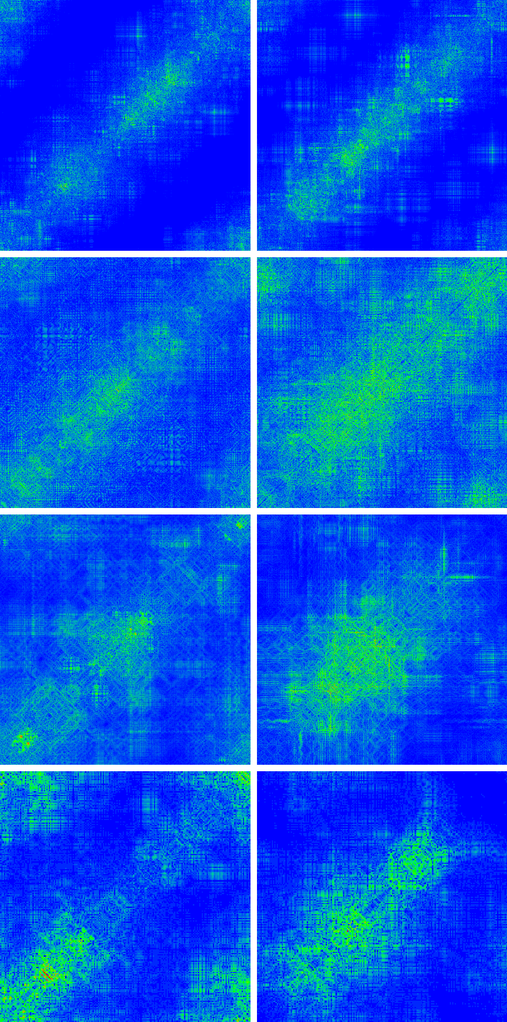
Figure 1: Density plot of typical delocalized eigenfunctions of (1) for $U=2$, $U_{R}=1$, energies close to $E=0$ (left) or $E=1$ (right), and $W=0.75$, $N=5000$ (first row), $W=1$, $N=1000$ (second row), $W=1.5$, $N=500$ (third row), $W=2.5$, $N=200$ (fourth row). The values of $\xi_{x}$, $\xi_{\rm CM}$, $\xi_{E}$, and $d_{\rm rel}$ are: first row: left: $\xi_{x}=3044.00$, $\xi_{\rm CM}=4993.33$, $\xi_{E}=221.53$, $d_{\rm rel}=288.11$, right: $\xi_{x}=2977.21$, $\xi_{\rm CM}=6033.04$, $\xi_{E}=167.82$, $d_{\rm rel}=344.77$, second row: left: $\xi_{x}=773.54$, $\xi_{\rm CM}=1336.25$, $\xi_{E}=100.99$, $d_{\rm rel}=99.65$, right: $\xi_{x}=804.24$, $\xi_{\rm CM}=1623.51$, $\xi_{E}=94.32$, $d_{\rm rel}=129.13$, third row: left: $\xi_{x}=305.00$, $\xi_{\rm CM}=505.15$, $\xi_{E}=55.83$, $d_{\rm rel}=55.94$, right: $\xi_{x}=215.75$, $\xi_{\rm CM}=378.44$, $\xi_{E}=55.35$, $d_{\rm rel}=57.65$, fourth row: left: $\xi_{x}=79.89$, $\xi_{\rm CM}=108.19$, $\xi_{E}=38.10$, $d_{\rm rel}=19.01$, right: $\xi_{x}=95.11$, $\xi_{\rm CM}=158.41$, $\xi_{E}=42.09$, $d_{\rm rel}=16.21$. The two axes correspond to the two particle positions $x_{1}$ and $x_{2}$. Red/green/blue corresponds to maximum/medium/minimum values of $|\psi(x_{1},x_{2})|$.

Figure 1 shows for certain cases with $200\leq N\leq 5000$ color density plots of typical rather strongly delocalized two-particle eigenfunctions of the TIP Hamiltonian (1) with values of $\xi_{x}$ and $\xi_{\rm CM}$ rather close to the system size $N$ despite the fact that the choice of the disorder parameter implies approximately $N\approx 11\,L_{1}$ (for the cases with $N\leq 1000$) or even $N\approx 27\,L_{1}$ (for the case $N=5000$). These states are more concentrated close to the diagonal which is confirmed by the observation that their values of $d_{\rm rel}$ are comparable to $L_{1}$. Furthermore, the internal structure of the eigenfunctions is quite complicated with many holes also close to the diagonal. Sometimes, especially for $E=1$, one can see certain horizontal and vertical structures which indicate a contribution of a non-interacting product eigenstate where $L_{1}$ for one particle is considerably stronger or weaker than $L_{1}$ for the other particle. The values of $\xi_{E}$ are always very clearly above unity, indicating a strong mixing or delocalization, We mention that the precise form for other examples of delocalized eigenstates varies very strongly, with a rich structure and sometimes even the overall cigar-shape along the diagonal is not very clearly visible.

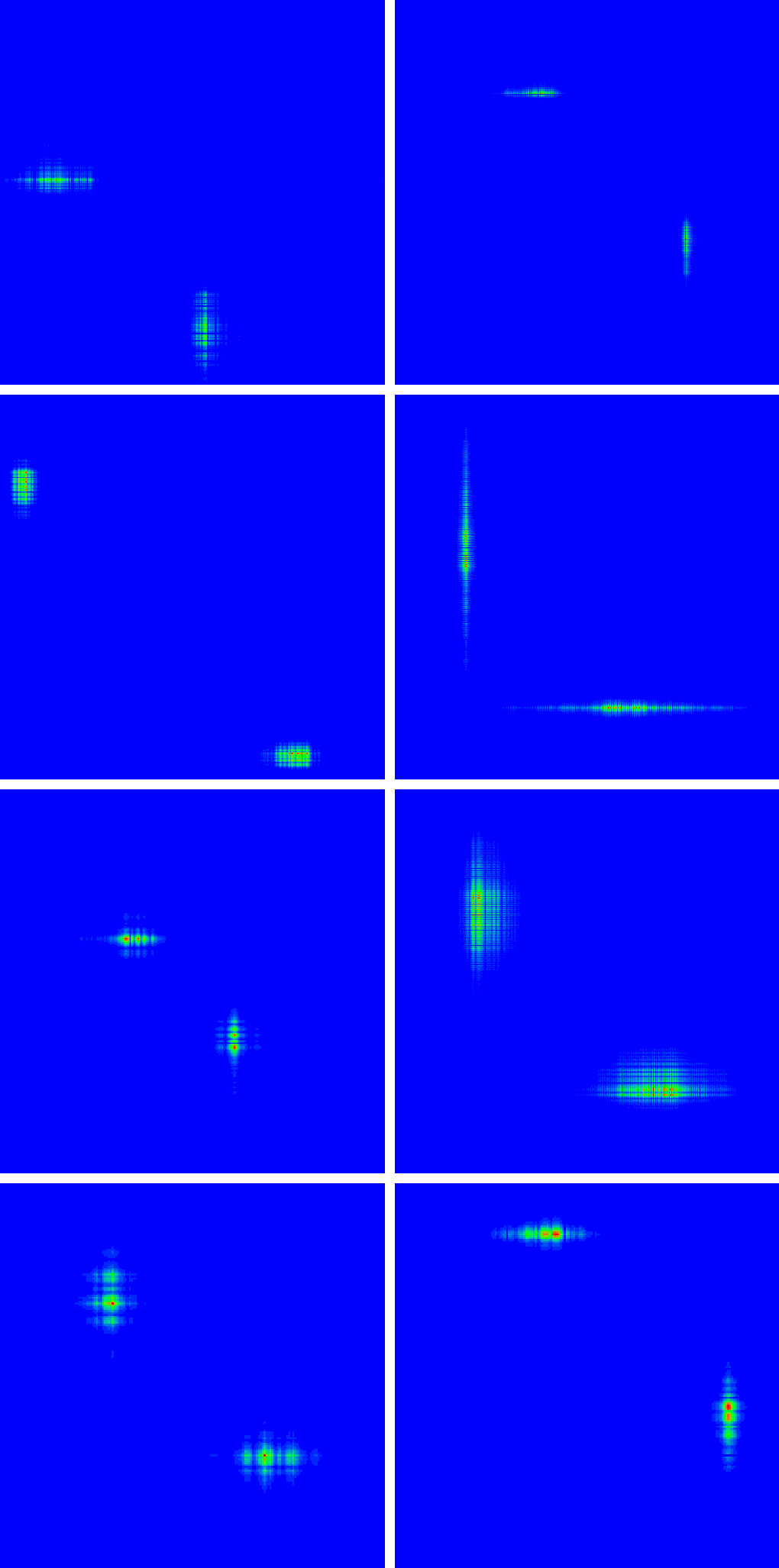
Figure 2: Density plot of typical localized product eigenfunctions of (1) with $\xi_{E}=1$ (with a numerical error below $10^{-7}$) for $U=2$, $U_{R}=1$, energies close to $E=0$ (left) or $E=1$ (right), and same values of $W$ and $N$ as in Figure 1 for corresponding rows. The values of $\xi_{x}$, $\xi_{\rm CM}$, and $d_{\rm rel}$ are: first row: left: $\xi_{x}=125.35$, $\xi_{\rm CM}=395.36$, $d_{\rm rel}=1947.08$, right: $\xi_{x}=57.42$, $\xi_{\rm CM}=264.38$, $d_{\rm rel}=1898.33$, second row: left: $\xi_{x}=51.81$, $\xi_{\rm CM}=73.02$, $d_{\rm rel}=290.64$, right: $\xi_{x}=27.80$, $\xi_{\rm CM}=105.41$, $d_{\rm rel}=408.16$, third row: left: $\xi_{x}=18.40$, $\xi_{\rm CM}=23.67$, $d_{\rm rel}=133.56$, right: $\xi_{x}=32.86$, $\xi_{\rm CM}=92.06$, $d_{\rm rel}=231.51$, fourth row: left: $\xi_{x}=8.20$, $\xi_{\rm CM}=9.24$, $d_{\rm rel}=80.91$, right: $\xi_{x}=10.59$, $\xi_{\rm CM}=11.82$, $d_{\rm rel}=92.01$. The two axes correspond to the two particle positions $x_{1}$ and $x_{2}$. Red/green/blue corresponds to maximum/medium/minimum values of $|\psi(x_{1},x_{2})|$.

For comparison we show in Figure 2 for the same parameters as in Figure 1 typical localized product eigenstates where $\xi_{E}$ is rather precisely unity and where both particles are localized far away such that the interaction does not significantly influence these type of states. The Green function Arnoldi method has apparently no problem in correctly identifying such states, which form actually the majority of found eigenstates for $N\gg L_{1}$. Their values of $\xi_{x}$ and $\xi_{\rm CM}$ are comparable to $L_{1}$ while now $d_{\rm rel}$, the average particle distance, is significantly larger than $L_{1}$. Sometimes, especially for $E=1$, one can see that the one-particle localization length for one particle is considerably larger than for the other particle. We mention that for these kind of states the values of $\xi_{x}$ and $\xi_{\rm CM}$ exhibit still quite large statistical fluctuations (but still comparable to $L_{1}$) due to the fluctuations of the IPR for the one-particle 1d-Anderson model without interaction.

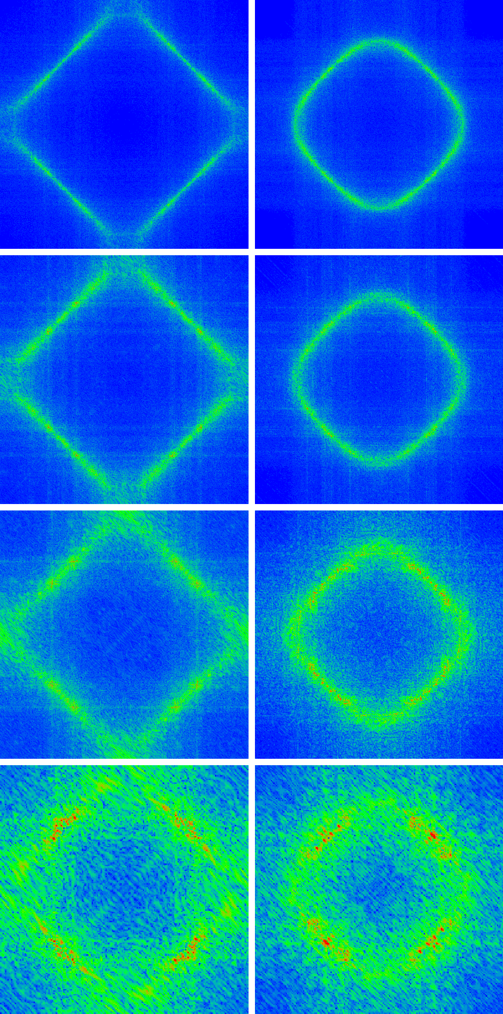
Figure 3: Density plot in momentum representation of the eigenstates of (1) of Figure 1 (same eigenstates for corresponding panels). The two axes correspond to the two particle momenta $k_{1}$ and $k_{2}$. Red/green/blue corresponds to maximum/medium/minimum values of $|\bar{\psi}(k_{1},k_{2})|$ with $\bar{\psi}(k_{1},k_{2})$ being the discrete Fourier transform of $\psi(x_{1},x_{2})$.

We also determined the wave function $\bar{\psi}(k_{1},k_{2})$ in momentum representation obtained by a standard 2d-discrete Fourier transform from $\psi(x_{1},x_{2})$ and with discrete values $k_{j}=2\pi p_{j}/N$, $p_{j}=0,\,\ldots,\,N-1$ for the momenta. Figure 3 shows density plots of this quantity for the same eigenstates of Figure 1 (for corresponding panels). The amplitudes in momentum representation are maximal for momenta close to the Fermi surface of the 2d tight-binding model (without disorder/interaction), i. e. $-2\cos(k_{1})-2\cos(k_{2})\approx E$ for the two cases $E=0$ (square form with sides parallel to the diagonals) or $E=1$ (a closed curve a bit similar to but still different from a circle).

To understand this we remind that in the weak disorder limit the one-particle eigenfunctions $\phi_{\nu}(x)$ of the 1d-Anderson model (2) have quite well defined momenta $k$ with $\epsilon_{\nu}\approx-2\cos(k)$ and the momentum fluctuations due the finite localization length $\sim L_{1}$ are of order $\Delta k\sim 1/L_{1}$ ponomarev1 implying a one-particle (disorder-induced) Breit-Wigner width $\Gamma_{W}\sim 1/L_{1}$ such that momenta with $|\epsilon_{\nu}+\cos(k)|<\Gamma_{W}$ contribute to the discrete Fourier expansion of $\phi_{\nu}(x)$. Furthermore, in energy representation (6) of a two-particle eigenstate essentially only non-interacting product eigenstates with $|E-(\epsilon_{\nu_{1}}+\epsilon_{\nu_{2}})|<\Gamma_{U}$ contribute where $\Gamma_{U}$ is the (interaction induced) Breit-Wigner width roughly given by $\Gamma_{U}\sim c(U)/L_{1}$ with a function $c(U)\sim|U|$ for small to modest values of $|U|$ jacquod2 ; frahm5 .

In total this implies that in momentum representation momenta obeying $|E+2\cos(k_{1})+2\cos(k_{2})|<\Gamma_{\rm tot}$ contribute to the two-particle eigenstate of (1) where $\Gamma_{\rm tot}\approx\Gamma_{U}+\,2\Gamma_{W}\sim 1/L_{1}\sim W^{2}$ is somewhat the total momentum Breit-Wigner width. The dependence of this width on $L_{1}$ or $W$ is very clearly visible in Figure 3 with quite sharply defined curves for $W=0.75$ (top panels in Figure 3) and quite thick curves for $W=2.5$ (bottom panels in Figure 3). For the case $E=0$ the effective width close to the corners of the square (with one momentum close to $\pi$ and the other one close to $0$ or $2\pi$) seems strongly enhanced which can be understood by the strongly reduced one-particle localization length $\tilde{L}_{1}\approx L_{1}\sin^{2}(k_{1,2})\ll L_{1}$ for both particles implying a strongly enhanced momentum uncertainty and therefore increasing the effective value of $\Gamma_{W}$.

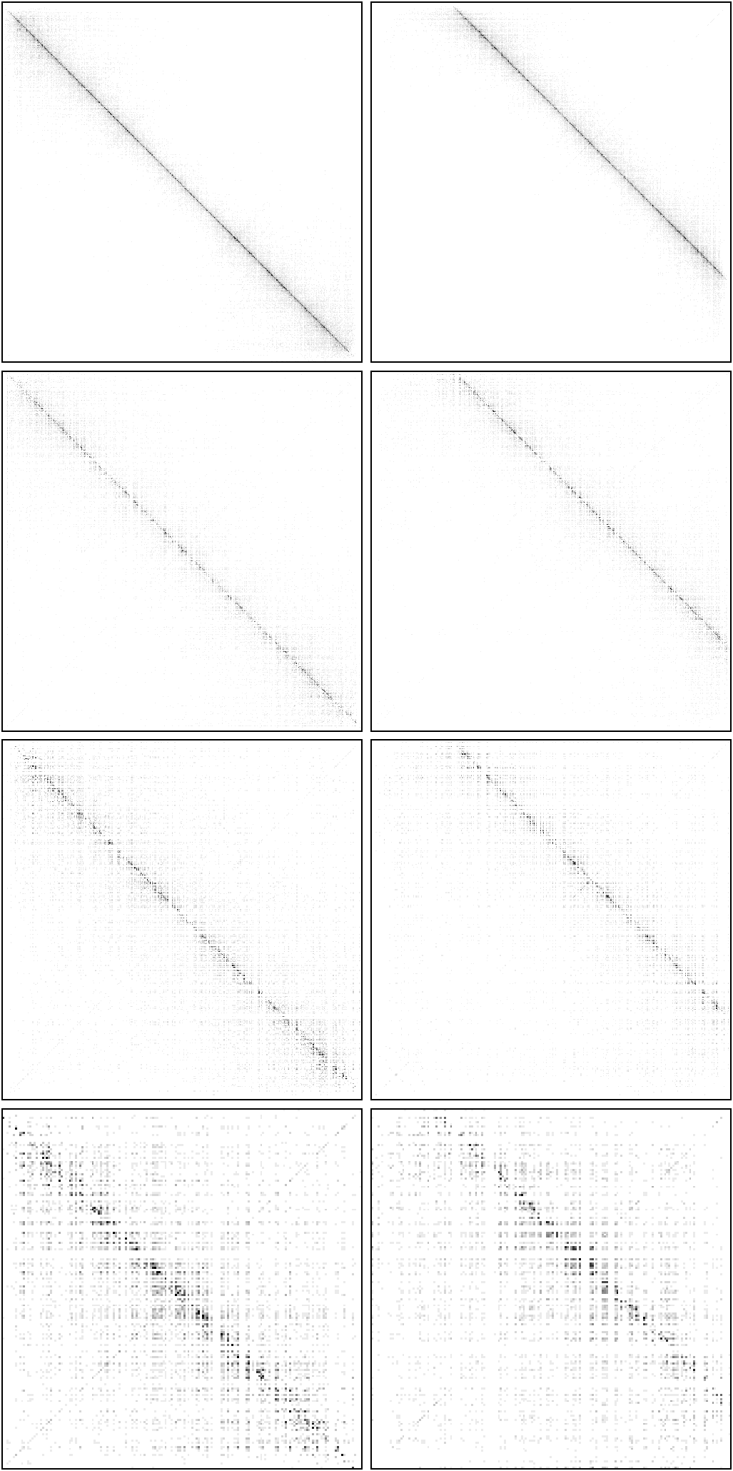
Figure 4: Grey scale density plot in one-particle energy representation (6) of the eigenstates of (1) of Figure 1 (same eigenstates for corresponding panels). Both axes correspond to the (one-particle) energies $\epsilon_{\nu_{1}}$ and $\epsilon_{\nu_{2}}$ of the two particles. The pixel size corresponds to the average level spacing in the band center of non-interacting one-particle energies $\epsilon_{\nu}$ (cases with $N\leq 1000$, second to fourth rows). This representation implies a slight coarse-graining if due to fluctuations several one-particle energies correspond to the same cell. The pixel size for the case $N=5000$ (top row) corresponds to 5 times the average level spacing in the band center implying a stronger coarse-graining for a better visibility. Black/grey/white corresponds to maximum/medium/minimum values of $|\chi_{\nu_{1},\nu_{2}}|$.

To illustrate the effect of the interaction induced Breit-Wigner width $\Gamma_{U}$ we show in Figure 4 density plots of the wave function in energy representation (6) for the same eigenstates of Figure 1 (for corresponding panels). The two axes correspond the one-particle energies $\epsilon_{\nu_{1}}$ and $\epsilon_{\nu_{2}}$ with a pixel size corresponding to the average level spacing of $\epsilon_{\nu}$ in the band-center of (2) for the three bottom panels with $N\leq 1000$. In this way in average a pixel corresponds approximately to one value of $\epsilon_{\nu}$. However, due to fluctuations of the one-particle energies and a reduced level spacing at the band edges there is a slight coarse-graining, with either some empty cells or a few values of $\epsilon_{\nu}$ for other cells. For the case $N=5000$ with such a representation the black pixels for maximum values would only be barely visible. Therefore we have applied for this case (shown in the top panels) a somewhat stronger coarse-graining using a pixel size of 5 times the average level spacing in the band center.

One can clearly see that the maximal contributions in energy representation correspond to the lines $E\approx\epsilon_{\nu_{1}}+\epsilon_{\nu_{2}}$ confirming the expected condition $|E-(\epsilon_{\nu_{1}}+\epsilon_{\nu_{2}})|<\Gamma_{U}$ with the interaction induced Breit-Wigner width $\Gamma_{U}$. Furthermore, one can also observe that the effective width of the lines increases with decreasing values of $L_{1}$ (or increasing values of $W$ from top to bottom panels) which is in qualitative agreement with $\Gamma_{U}\sim 1/L_{1}\sim W^{2}$ which is similar to the width $\Gamma_{\rm tot}$ visible in Figure 3 but still with a considerably smaller numerical prefactor for $\Gamma_{U}$ as compared to $\Gamma_{\rm tot}$. We note that in principle, and without the coarse-graining, the quantity $\xi_{E}$ would correspond the number of black pixels in Figure 4. This figure clearly confirms the Breit-Wigner type “energy space localization” one can find in random band matrix models with a strong diagonal jacquod1 ; fyodorov1 ; frahm2 even though the interaction dependence of $\Gamma_{U}$ for the TIP problem is different as predicted in such models due to the (somewhat incorrect) assumption of random uniform distributions of interaction coupling matrix elements for the latter.

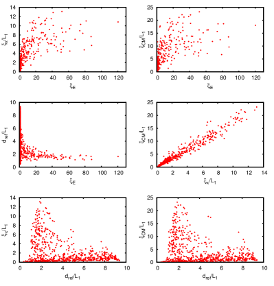
Figure 5: Pairwise cross dependence of the four quantities $\xi_{x}/L_{1}$, $\xi_{\rm CM}/L_{1}$, $d_{\rm rel}/L_{1}$ and $\xi_{E}$ computed for the $657$ eigenstates with energies closest to $E=0$ for one particular disorder realization of the Hamiltonian (1) for $U=2$, $U_{R}=1$, $N=2000$ and $W=1$. $L_{1}$ is the corresponding one-particle localization length $L_{1}=105$. Each of the panel shows the dependence of one of these four quantities on one of the other three quantities providing 6 combinations.

The physical picture of the TIP delocalization effect described in dlstip is that the delocalized TIP eigenstates in position representation show also a strong delocalization in energy representation and contain only non-interacting pair eigenstates where both particles have a typical distance $\sim L_{1}$. Other non-interacting pair eigenstates with particles distances $\gg L_{1}$ are essentially untouched by the interaction and are therefore perfectly localized in energy representation with $\xi_{E}=1$. Figure 5 illustrate these points rather clearly by showing the cross-dependencies of all combinations between two of the four quantities $\xi_{x}/L_{1}$, $\xi_{\rm CM}/L_{1}$, $d_{\rm rel}/L_{1}$ and $\xi_{E}$ obtained from $657$ eigenstates with energies close to $E=0$ for one particular disorder realization of the Hamiltonian (1) for $N=2000$ and $W=1$.

The two quantities $\xi_{x}$ and $\xi_{E}$ seem to be loosely correlated in the sense that large values of $\xi_{E}$ imply larger values of the ratio $\xi_{x}/L_{1}$ but there are statistical fluctuations with $\xi_{x}/L_{1}$ being large for modest values of $\xi_{E}$ and vice-versa. For example the eigenstate with maximal $\xi_{E}\approx 120$ corresponds to $\xi_{x}\approx 11L_{1}$ while there is another eigenstate with a considerably smaller value $\xi_{E}\approx 25$ and still $\xi_{x}\approx 12L_{1}$. Localized pair states with $\xi_{E}\approx 1$ correspond to small values of $\xi_{x}/L_{1}$ of order unity but statistical fluctuations of the one-particle IPR allow for values up to $4$-$5$ of the latter. The behavior for the dependence of $\xi_{\rm CM}$ on $\xi_{E}$ is rather similar with values of $\xi_{\rm CM}$ that are roughly twice the values of $\xi_{x}$.

The dependence of the average particle distance $d_{\rm rel}$ on $\xi_{E}$ is rather clear. Large values of $d_{\rm rel}\gg L_{1}$ are only possible for $\xi_{E}\approx 1$ corresponding to pair localized eigenstates and large values of $\xi_{E}$ imply values of $d_{\rm rel}/L_{1}$ between $1$-$2$.

The two quantities $\xi_{\rm CM}$ and $\xi_{x}$ are rather well correlated and the expected behavior $\xi_{\rm CM}\approx 2\xi_{x}$ is indeed quite well verified in average. However, also here we observe some significant statistical deviations, probably due to some particular effects of the shape of the eigenstate, if it is closer to a cigar form or a more bulky shape.

The dependence of $\xi_{x}$ ($\xi_{\rm CM}$) on $d_{\rm rel}$ is somewhat similar to the dependence of $\xi_{E}$ on $d_{\rm rel}$, i. e. large values $\xi_{x}\gg L_{1}$ ($\xi_{\rm CM}\gg L_{1}$) require $d_{\rm rel}\sim L_{1}$ and large values $d_{\rm rel}\gg L_{1}$ correspond to $\xi_{x}\sim L_{1}$ ($\xi_{\rm CM}\sim L_{1}$). However, the statistical fluctuations with respect to these two limits are considerably stronger as compared to the dependence of $\xi_{E}$ on $d_{\rm rel}$.

The results for exact eigenstates of large TIP systems shown in this section illustrate and confirm quite clearly many of the physical properties concerning the TIP enhancement of the one-particle localization length as described in the early work dlstip ; jacquod1 ; fyodorov1 ; frahm2 provided that the functional dependence of the Breit-Wigner width is corrected taking into account realistic distributions of the interaction coupling matrix elements jacquod2 ; ponomarev1 ; frahm5 .

Higher quality gif files for the different panels of Figures 1 to 4 including color versions for the panels of Figure 4 are available for download at webpage .

4 Scaling of IPR

In this section we present and discuss results for the parameter dependence on disorder, interaction strength and range of the three IPR quantities $\xi_{x}$, $\xi_{\rm CM}$ and $\xi_{E}$ obtained from effective averages and finite size scaling of several disorder realizations. For this we compute appropriate finite size (harmonic) averages of these quantities for a selection of relevant TIP eigenstates corresponding to particle distances $\sim L_{1}$ for which the interaction induced enhancement effect is expected to be best visible dlstip . Explicitely, the relevant eigenstates are selected as the fraction $L_{1}/N$ of eigenstates with maximal values of $\xi_{E}$, the IPR in energy representation. This choice seems preferable to us since $\xi_{E}$ measures most directly the interaction induced delocalization effect while $\xi_{x}$ and $\xi_{\rm CM}$ are also influenced by the rather considerable statistical fluctuations of the one-particle localization lengths of the non-interacting product eigenstates. Actually Figure 5 shows that correlations of $\xi_{x}$ (or $\xi_{\rm CM}$) with $\xi_{E}$ are rather loose and therefore the eigenstates with maximal $\xi_{E}$ are not exactly the same as those with maximal $\xi_{x}$.

In absence of interaction we have precisely $\xi_{E}=1$ for all eigenstates and in order to be able to determine the set of relevant states for this particular case we chose $U=10^{-5}$ and not exactly $U=0$ as reference value for “vanishing interaction strength”. The small interaction value does not significantly modify the values of the IPR quantities but it ensures small differences of $\xi_{E}$ allowing to distinguish between the relevant eigenstates with $\xi_{E}$ slightly above unity, typically $\xi_{E}-1\sim 10^{-3}$, and non-relevant states corresponding to precisely $\xi_{E}=1$.

For each parameter set of $N$, $W$, $U$, $U_{R}$ and $E$ we computed about $\sim 650$ two-particle eigenstates (per disorder sample) by the Green function Arnoldi method using the Arnoldi dimension $n_{A}=1000$ and for 10 different disorder realizations providing $\sim 6500$ eigenstates in total per parameter set. For a fixed value of $N$ and different other parameters we always chose the same 10 disorder realizations, with the precision that “same disorder realization” for two different disorder values $W$ means a uniform scaling factor between the two disorder configurations. Then, as already explained, we selected for each sample the fraction of $L_{1}/N$ eigenstates with maximal values of $\xi_{E}$ as relevant states. Using these selected states we computed the inverse average (harmonic mean) to obtain the (inverse) size dependent “average values” for the three quantities $\xi_{x}$, $\xi_{\rm CM}$ and $\xi_{E}$. The corresponding statistical errors are typically between $1$% and $3$% and strangely here the relative errors are somewhat larger for stronger disorder or smaller interaction values.

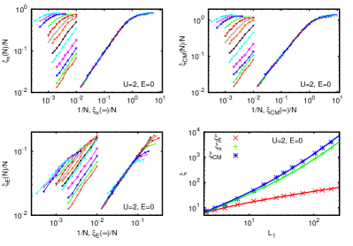
Figure 6: Illustration of the scaling procedure to determine the three inverse participation ratios $\xi_{x}$, $\xi_{\rm CM}$ and $\xi_{E}$ at infinite system size. Top left panel shows (in a double logarithmic scale) the rescaled finite size IPR $\xi_{x}(N)/N$ versus $1/N$ (left set of curves) and versus $\xi_{x}(\infty)/N$ (right set of curves) with $\xi_{x}(\infty)$ determined such that the data points are closest to a single scaling curve (approximately) shown by the blue curve corresponding to the fit (32). Top right (bottom left) panel shows the scaling for $\xi_{\rm CM}$ ($\xi_{E}$). The interaction strength is $U=2$, corresponds to the Hubbard short range interaction and the approximate energy is $E=0$. The used disorder values are $W=0.75,\,0.875,\,1,\,1.25,\,1.5,\,1.75,\,2,\,2.5,\,3,\,4,\,5,\,6,\,7$ with $W=0.75$ for the top curve and $W=7$ for the bottom curve. The range of system sizes is $100\leq N\leq N_{\rm max}$ with $N_{\rm max}=500$ (for largest values of $W$) or $N_{\rm max}=2000$ (for smallest values of $W$). For $W=0.75$ also one data point with $N=3000$ has been computed. For the scaling procedure only data points with $N\geq 2\,L_{1}$ have been used and are visible in top and bottom left panels. Bottom right panel shows (in a double logarithmic scale) the three infinite size IPR quantities obtained by finite size scaling versus $L_{1}=105/W^{2}$ (discrete data points). The continuous curves in this panel correspond to the fits: $\xi_{\rm CM}=a_{2}\,L_{1}+b_{2}\,L_{1}^{\gamma_{2}}$ with $a_{2}=3.10\pm 0.12$, $b_{2}=0.098\pm 0.038$, $\gamma_{2}=2.01\pm 0.09$ (top blue curve), $\xi_{x}=a_{1}\,L_{1}+b_{1}\,L_{1}^{\gamma_{1}}$ with $a_{1}=3.00\pm 0.12$, $b_{1}=0.043\pm 0.024$, $\gamma_{1}=2.04\pm 0.12$ (middle green curve) and $\xi_{E}=a_{3}+b_{3}\,L_{1}^{\gamma_{3}}$ with $a_{3}=-7.0\pm 1.6$, $b_{3}=10.4\pm 1.4$, $\gamma_{3}=0.35\pm 0.03$ (lower red curve).

For each set of different values of $E$, $U$, $U_{R}$, and eventual boson or fermion case, we determined the disorder dependent “infinite size” IPR by the procedure of one-parameter finite size-scaling mackinnon1 ; mackinnon2 ; kramer1 by fitting the data to a universal scaling function $f$ by :

$$\frac{\xi(N)}{N}=f\left(\frac{\xi(\infty)}{N}\right)$$ (20)

where $\xi(N)$ represents one of the three (size and disorder dependent) IPR quantities ($\xi_{x}$, $\xi_{\rm CM}$ or $\xi_{E}$) and $\xi(\infty)$ is the (disorder dependent) infinite size limit of $\xi(N)$ to be determined by the scaling procedure. Details of our implementation of this procedure are explained in Appendix A.

Concerning $W$ and $N$ we choose values in the range $0.75\leq W\leq 7$ (see caption of Figure 6 for the precise values) and $N_{\rm min}=100\leq N\leq N_{\rm max}$ with $N_{\rm max}=500$ (for largest values of $W$) or $N_{\rm max}=2000$ (for smallest values of $W$). For $W=0.75$ (and $U=2$, $U_{R}=1$, $E=0$) also one data point with $N=3000$ has been computed. For these parameters the scaling procedure works actually very well for $\xi_{x}$ and $\xi_{\rm CM}$ as can be seen in the top panels of Figure 6 valid for $U=2$, $U_{R}=1$ and $E=0$, and provided we only use data with $N\geq 2L_{1}$, (e. g. $N\geq 380$ for $W=0.75$) according to the discussion in Appendix C for the validity condition of the scaling approach. The scaling curves for these two quantities are very nice and we obtain reliable results for $\xi_{x}(\infty)$ and $\xi_{\rm CM}(\infty)$ with relative errors between $6$% and $8$% for the smallest disorder value $W=0.75$ (see Appendix A for the computation method of these errors). We mention that the few data points with $N<2L_{1}$ (not shown in Figure 6) for the smallest values of $W$ and $N$ are clearly below/outside the main scaling curve and do not obey one-parameter scaling.

The scaling for the third IPR quantity $\xi_{E}$ only works approximately for still larger values $N\geq 4L_{1}$ (bottom left panel of Figure 6) but since $\xi_{E}$ is not defined in terms of spatial positions we do not expect the scaling to be perfect. However, here the data for larger values of $N$ fall well on the lower linear part of the scaling curve where $f(x)\approx x$ for small $x$ corresponding to $\xi_{E}(N)\approx\xi_{E}(\infty)$. Since the scaling procedure optimizes just for this linear region it provides therefore correct results for the extrapolated infinite size values of $\xi_{E}$.

The bottom right panel of Figure 6 shows the dependence of the obtained infinite size IPR values on $L_{1}=105/W^{2}$ (for $U=2$, $U_{R}=1$ and $E=0$). For the two cases $\xi_{x}$ and $\xi_{\rm CM}$ the power law fit with finite size correction: $\xi_{x}=a_{1}L_{1}+b_{1}L_{1}^{\gamma_{1}}$ and $\xi_{\rm CM}=a_{2}L_{1}+b_{2}L_{1}^{\gamma_{2}}$ works very well with both exponents $\gamma_{1}=\gamma_{2}=2$ within the margin of error (see caption of Figure 6 for complete fit results) implying the scaling $\xi_{x,{\rm CM}}\sim L_{1}^{2}$ for the limit $L_{1}\to\infty$. For $\xi_{E}$ a modified power law fit with a constant term: $\xi_{E}=a_{3}+b_{3}L_{1}^{\gamma_{3}}$ works very well with $\gamma_{3}=1/3$ (and a negative value of $a_{3}$) within the margin of error implying the scaling $\xi_{E}\sim L_{1}^{1/3}$ for $L_{1}\to\infty$. This scaling is clearly below the estimation $\xi_{E}\sim L_{1}^{2}$ obtained in jacquod1 ; fyodorov1 ; frahm2 from the simplified band matrix model with preferential basis combined with the (incorrect) assumption of random and uniform distributions for the interaction coupling elements. We will come back to this point in Section 6.

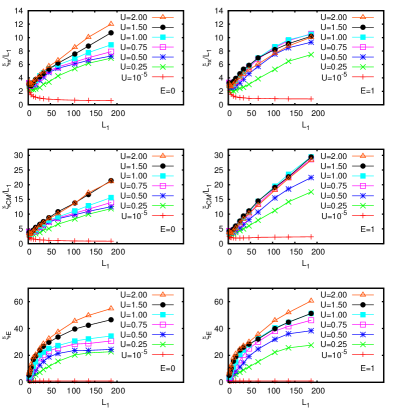
Figure 7: Dependence of the three quantities $\xi_{x}/L_{1}$ (top panels), $\xi_{\rm CM}/L_{1}$ (center panels) and $\xi_{E}$ (bottom panels), obtained by finite size scaling, on the one-particle localization length $L_{1}=105/W^{2}$ for the same disorder values used in Figure 6, the interaction values $U=10^{-5},\,0.25,\,0.5,\,0.75,\,1,\,1.5,\,2$ for the Hubbard interaction and the two energy values $E=0$ (left panels) and $E=1$ (right panels).

These first results are however specific to the case $U=2$, $U_{R}=1$ and $E=0$. Figure 7 shows for $E=0$ and $E=1$ the dependence of the enhancement factors $\xi_{x}/L_{1}$, $\xi_{\rm CM}/L_{1}$, and of $\xi_{E}$ (all obtained by finite size scaling) on $L_{1}$ for $U_{R}=1$ and several values of $0<U\leq 2$ including the reference value $U=10^{-5}$ for “vanishing interaction strength”. For the energy $E=0$ the IPR values increase with increasing interaction strength and the dependence $\xi_{x,{\rm CM}}/L_{1}\sim L_{1}+$const. only applies to the strongest interaction values $U=1.5$ and $U=2$ while for smaller interaction values the behavior is sublinear. The behavior of $\xi_{E}$ is always clearly sublinear and for the smallest interaction values one may even observe a saturation with increasing $L_{1}$. For the other energy $E=1$ the situation is more complicated. First the dependence of $\xi_{x,{\rm CM}}$ is not clearly monotonic for all shown interaction values and a linear behavior is only observed for $\xi_{\rm CM}/L_{1}$ but here for a larger interval $0.75\leq U\leq 2$ of interaction values. Furthermore both $\xi_{x}/L_{1}$ and $\xi_{\rm CM}/L_{1}$ seem not to depend strongly on the interaction for this interval. For $\xi_{E}$ the behavior is also sublinear but for $U=2$ the exponent $\gamma_{3}$ (of the power law fit with constant term) is close to $1/2$ within the margin of error (instead of $1/3$ for $E=0$). The discussion of the particular case $U=10^{-5}\approx 0$ (curve closest to the bottom of each panel) is given in Appendix B.

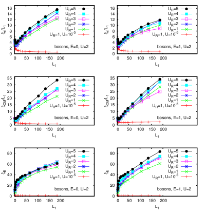
Figure 8: Dependence of the three quantities $\xi_{x}/L_{1}$ (top panels), $\xi_{\rm CM}/L_{1}$ (center panels) and $\xi_{E}$ (bottom panels), obtained by finite size scaling, on the one-particle localization length $L_{1}=105/W^{2}$ for the same disorder values used in Figure 6, the interaction value $U=2$ with the boson case and interaction ranges $U_{R}=1,\,2,\,3,\,4,\,5$ and the two energy values $E=0$ (left panels) and $E=1$ (right panels). For comparison also the data for $U=10^{-5}$ and $U_{R}=1$ are shown.

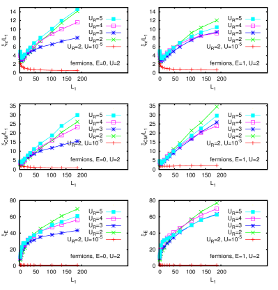
Figure 9: Same as Figure 8 but for the fermion case with $U_{R}=2,\,3,\,4,\,5$ and the additional data for $U=10^{-5}$ corresponds to $U_{R}=2$.

We have also studied the case of longer interaction ranges with $2\leq U_{R}\leq 5$ for a uniform interaction strength $U=2$ and both boson and fermion cases with the results shown in Figures 8 and 9. For comparison both figures also show data for the reference value $U=10^{-5}$ with $U_{R}=1$ (or $U_{R}=2$) for bosons (fermions). For bosons the results are rather similar to the case $U=2$ of Figure 7 with somewhat larger enhancement factors $\xi_{x}/L_{1}$, $\xi_{\rm CM}/L_{1}$ for longer interaction ranges and a dependence on $L_{1}$ between sublinear and linear. For $\xi_{E}$ the delocalization effect happens quite abruptly already for quite small values of $L_{1}$ for the largest interaction range $U_{R}=5$ and seems to follow a shifted linear dependence. The power law fits with constant term, $\xi_{E}=a_{3}+b_{3}\,L_{1}^{\gamma_{3}}$, provide for the range $20\leq L_{1}\leq 200$ and for bosons $\gamma_{3}=0.62\pm 0.05$ ($\gamma_{3}=0.89\pm 0.05$) for $E=0$ ($E=1$). For fermions the results are a bit similar to the boson case but with the strongest enhancement corresponding either to $U_{R}=5$ or $U_{R}=2$. Here the same type of fits for $\xi_{E}$ provide $\gamma_{3}=0.50\pm 0.07$ ($\gamma_{3}=0.70\pm 0.09$) for $E=0$ ($E=1$).

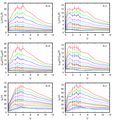
Figure 10: Interaction dependence of the three quantities $\xi_{x}(U)/\xi_{x}(0)$ (top panels), $\xi_{\rm CM}(U)/\xi_{\rm CM}(0)$ (center panels) and $\xi_{E}(U)$ (bottom panels) obtained by finite size scaling for $0<U\leq 12$, the Hubbard interaction and the two energy values $E=0$ (left panels) and $E=1$ (right panels). The reference values $\xi_{x}(0)$ and $\xi_{\rm CM}(0)$ have been computed using the interaction value $U=10^{-5}\approx 0$. Note that the corresponding reference value for $\xi_{E}$ at $U=10^{-5}$ is numerically very close to unity: $|\xi_{E}(0)-1|<10^{-3}$. The different curves correspond to different disorder values (same values as in Figure 6) with $W=0.75$ for the top curve and $W=7$ for the bottom curve. All panels show error bars for data in the range $2\leq U\leq 4$.

In Figure 10 the interaction dependence of the enhancement factors $\xi_{x}(U)/\xi_{x}(0)$, $\xi_{\rm CM}(U)/\xi_{\rm CM}(0)$, and of $\xi_{E}(U)$ for $U_{R}=1$ and several disorder values is shown where $\xi_{x}(0)$ and $\xi_{\rm CM}(0)$ have been computed using the interaction value $U=10^{-5}$ $\approx 0$. For $E=0$ the interaction induced enhancement sets already in for $U\geq 0.1$ with enhancement factors between $10$-$15$ and $\xi_{E}\approx 20$. Then there is a region of maximum enhancement $2\leq U\leq 4$ with enhancement factors between $22$-$30$ and $\xi_{E}\approx 60$. Then for $U>4$ the enhancement factors and $\xi_{E}$ decay (at $U=12$) to values between one third and one half of the maximum values at $U=3$-$4$ in agreement with the predicted vanishing of the enhancement effect for $U\gg 1$ predicted in ponomarev1 . For $E=1$ the overall behavior is similar but the effect of a strong enhancement already at $U=0.1$ is even stronger and the maximum region is extended to $0.5\leq U\leq 4$. However, the maximum enhancement factors are reduced to values $12$-$13$ due to enhanced values of $\xi_{x}(0)$ and $\xi_{\rm CM}(0)$. We remind that, according to Figure 7, the enhancement factor for $E=1$ is comparable or even slightly larger as the case $E=0$ when it is measured with respect to $L_{1}$ and not to $\xi_{x}(0)$ or $\xi_{\rm CM}(0)$.

We mention that for $U=2$, $U_{R}=1$ we also computed two set of data points at very small disorder $W=0.5$ and $W=0.625$ with $100\leq N\leq N_{\rm max}=2000$. It turns out that the scaling for this additional data is very problematic and the scaling curve for $W=0.5$ does not even overlap (in vertical direction) with the previous curves such at best one could try a scaling with an extrapolation of the last scaling curve. Due to this we omit these data sets and limit ourselves to $W\geq 0.75$ as far the IPR quantities are concerned.

The results of this section clearly that show the interaction induced enhancement of the two-particle localization length, measured by $\xi_{x}/L_{1}$ and $\xi_{\rm CM}/L_{1}$ using optimal interaction values, behaves as $\sim L_{1}+$const.

5 Green function localization length

In this section we consider the boson case with the Hubbard interaction $U_{R}=1$ and open boundary conditions (in contrast to the eigenfunction calculations of the last two sections with periodic boundary conditions) and we study the localization length defined by the exponential decay of the projected Green function $\bar{G}(x,y)$ given as $<\!x,x|G|y,y\!>$ between configurations where both particles are on the same site $x$ or $y$. First, one should note that even though the computational methods for the projected Green function used in song1 ; leadbeater1 are different, less effective than our method based on Eq. (11) (see Section 2), they should provide identical results provided that the numerical implementation is stable and sufficiently accurate.

Let us assume that we have computed the projected Green function for many different disorder realizations of samples of size $N$, for identical other parameters ($E$, $U$, etc.) and for some values $x$ close to one border at $0$ and $y$ being close to the other border at $N-1$. Then we define the rather general length scale $L_{G}$ depending on several parameters by

$$\frac{1}{L_{G}(x,y,N,\kappa)}=-\left\langle\frac{1}{y-x}\,\ln\left(\frac{|\bar{G}(x,y)|}{|\bar{G}(x,x)|^{\kappa}}\right)\right\rangle_{W}$$ (21)

where $\langle(\cdots)\rangle_{W}$ represents the ensemble average with respect to different disorder realizations. The parameter $\kappa$ is chosen either $1$ or $0$ depending if we want to take into account or not a finite size correction by the extra contribution of $|\bar{G}(x,x)|$ in the denominator. Furthermore, let $L^{-1}_{\rm av}(x,N,\kappa)$ be defined as the average of (21) with respect to 10% of $y$-values close to the second border $N-1$, i. e.: $N-N/10\leq y<N$. The hope behind this average in $y$ is to reduce short range fluctuations in the projected Green function due to the ballistic behavior for small length scales and small disorder values. In frahm5 we used the quantity

$$L_{2}(N)=L_{\rm av}(N/20,N,1)$$ (22)

using the average for $y$, the position $x=N/20$ and the choice with denominator $|\bar{G}(x,x)|$ to define “the” finite size two-particle Green function localization length called $L_{2}$. In song1 the quantity $L_{G}(0,N-1,N,0)$ was used, i. e. using the choice $x=0$, $y=N-1$ and without the denominator $|\bar{G}(x,x)|$ while in leadbeater1 apparently the quantity $L_{G}(p,N-1-p,N,0)$ (or similar) was used where both positions $x$ and $y$ are taken slightly inside the sample (at $x=p$ and $y=N-1-p$ for some suitable small value of $p$) to reduce possible boundary effects.

In the limit of samples in the strongly localized regime, with $N$ being much larger than the two-particle localization length, and assuming only small particular boundary effects (a problematic assumption as we will see) one would expect that $L_{G}$ and $L_{\rm av}$ provide identical localization lengths for reasonable parameter choices for the two positions $x$, $y$ and the parameter $\kappa=0$ or $1$. However, in realistic situations, when trying to compute the infinite size localization length by finite size scaling and for small disorder values, the size $N$ is comparable or even quite smaller than the two-particle localization length. In this regime the precise choice of parameters $x$, $y$ and $\kappa$ may indeed have an important impact on the results.

To test the effect of this we have therefore simultaneously computed eight quantities $L_{G}(0,N-1,N,\kappa)$ (both positions at the boundary), $L_{G}(N/20,N-1-N/20,N,\kappa)$ (both positions 5% inside the boundary), $L_{\rm av}(0,N,\kappa)$ ($x$ at the boundary and 10% average for $y$ at the other boundary), and $L_{\rm av}(N/20,N,\kappa)$ ($x$ 5% inside the boundary and 10% average for $y$ at the other boundary), for both values $\kappa=0$ and $\kappa=1$, several interaction values, and $E=0$ or $E=1$.

Then we have applied finite size scaling, using the automatic procedure described in appendix A, to the raw data to determine the associated infinite size localization lengths for each quantity. For this we used 15 disorder values in the range $0.5\leq W\leq 7$ (see caption of Figure 11 for precise values) and system sizes in the range $N_{\rm min}=50\leq N\leq N_{\rm max}$ with $N_{\rm max}=215$ (for largest values of $W$) and $N_{\rm max}=2000$ (for smallest values of $W$). The density of $N$-values corresponds to an approximate factor of $1.2$ between two neighbor values of $N$. For the scaling procedure we also limited ourselves to data points with $N\geq 1.5L_{1}$ since according to the discussion of Appendix C $N$ must be larger than $L_{1}$ for the validity of the one-parameter scaling hypothesis. The average over different disorder realization has been performed up to a precision of 1% or better for six interaction values $U\in\{0.25,\,0.5,\,0.75,\,1,\,1.5,\,2\}$ which requires 20 samples for $W=7$ at $N=215$, $E=0$ (minimum number) and $\approx 1.3\times 10^{5}$ samples for $W=0.5$, $N=50$, $E=1$ (maximum number).

For $E=0$ we find that for all eight cases the scaling procedure works very well with well defined scaling curves. The 4 cases with one or two positions exactly at the boundary produce (for smallest values of $W$) rather considerable variations of the infinite size localization length while the values for the 4 cases with one or two positions 5% inside the boundary are somewhat smaller but also closer together. Furthermore, the cases $\kappa=1$ [i.e. “with” the denominator $|\bar{G}(x,y)|$ in (21)] produce at same system size $N$ larger values as the cases with $\kappa=0$ which is not a problem as such if after finite size scaling the results are coherent. However, due to this for $\kappa=1$ the scaling curves for small $W$ are a bit lower (not in the flat regime of the scaling curve) with stronger slopes such the scaling is more reliable. For $E=1$ the situation is somewhat similar but here the two cases without average for the $y$-position and with both positions at the boundary do not scale correctly and the individual curves cannot be matched to one scaling function (for $U=2$). The other six cases with either average or positions 5% inside the boundary produce rather nice scaling curves but here the condition $N\geq 1.5L_{1}$ is indeed important, actually somewhat more important than for the case $E=0$. Furthermore, for $U=0$ we have the impression that the cases with average produce a smaller variation for the dependence on $L_{1}$ which seems more reasonable to us. Therefore, in summary we choose for this work (and except the particular cases studied in Appendix C) the case with average, with $\kappa=1$ and the $x$-position 5% inside the boundary, i. e. we stick to our initial choice frahm5 with $L_{2}$ given by (22).

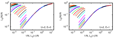
Figure 11: Illustration of the scaling procedure to determine the Green function two-particle localization length $L_{2}$ at infinite system size for $U=2$ and energy values $E=0$ (left panel) and $E=1$ (right panel). Both panels show (in a double logarithmic scale) $L_{2}(N)/N$ versus $1/N$ (left set of curves) and versus $L_{2}(\infty)/N$ (right set of curves) with $L_{2}(\infty)$ determined such that the data points are closest to a single scaling curve (approximately) shown by the blue curve corresponding to the fit (32). $L_{2}(N)$ has been computed from (22) as explained in the text. The used disorder values are $W=0.5,\,0.625,\,0.75,\,0.875,\,1,\,1.25,\,1.5,\,1.75,\,2,\,2.5,\,3,\,4,\,5,\,6,\,7$ with $W=0.5$ for the top curve and $W=7$ for the bottom curve. The used values for the system size $N$ are between $N_{\rm min}=50$ and $N_{\rm max}=215$ (for largest values of $W$) and $N_{\rm max}=2000$ (for smallest values of $W$). Only data points with $N\geq 1.5\,L_{1}$ have been used for the scaling procedure and are shown in the figure.

Figure 11 illustrates the scaling procedure for this quantity and the case $U=2$ and both energies $E=0$ and $E=1$. The quality of the two scaling curves is very impressive and appears even better than the quality of the scaling curves of the IPR quantities shown in Figure 6. The two-particle localization lengths $L_{2}$ for infinite system size obtained from this coincide (for the case $E=0$) within the margin of error with our previous results frahm5 for disorder values $1\leq W\leq 7$ and obtained by finite size extrapolation using data with $100\leq N\leq 1400$. However, our results deviate considerably from those of song1 ; leadbeater1 which we attribute to the limited system sizes $N\lesssim 250$ used in these two works not respecting the condition $N>L_{1}$ of the one-parameter scaling approach kramer1 for smaller disorder values. A detailed analysis of this point by simulating different scaling scenarios for limited system size and other parameters used in (21) is given in Appendix C. In this appendix also discrepancies between song1 and leadbeater1 are explained by another scaling related problem.

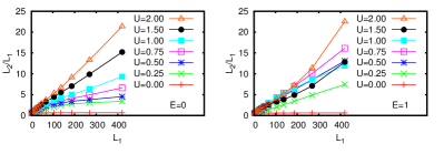
Figure 12: Enhancement factor $L_{2}/L_{1}$ versus $L_{1}=105/W^{2}$ for $U=0,\,0.25,\,0.5,\,0.75,\,1,\,1.5,\,2$ and energy $E=0$ ($E=1$) for left (right) panel. The used disorder values $W$ are as in Figure 11.

In the following (and except Appendix C) the quantity $L_{2}$ always denotes the infinite size localization length obtained by finite size scaling from $L_{2}(N)$ defined in (22). Figure 12 shows the dependence of the enhancement factor $L_{2}/L_{1}$ on $L_{1}$ for certain selected interaction values in a similar way as in Figure 7. For $E=0$ we see a linear behavior for larger interaction values and sublinear form for smaller interaction strengths and the overall dependence on $U$ is clearly monotonic. We mention that the approximate formula $L_{2}\approx L_{1}/2+c(U)L_{1}^{2}$ with $c(U)\approx 0.074\,|U|/(1+|U|)$ suggested in frahm5 works rather well for disorder values $W>1$ and $|U|\leq 2$ corresponding to the available data of frahm5 . However for smaller disorder values, there are significant deviations due to the cases of sublinear behavior. For $E=1$ the situation is more complicated with even stronger than linear behavior for certain interaction values and the $U$-dependence is not monotonic. In particular the enhancement factor is quite reduced for $U=1$ and $U=1.5$ if compared to $U=2$ and $U=0.75$. This strange behavior will be better clarified below in the discussion of Figure 15. As for the IPR quantities the discussion of the particular case $U=0$ (curve closest to the bottom of each panel) is given in Appendix B.

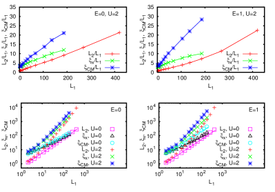
Figure 13: Top panels: Comparison of the dependence of $L_{2}/L_{1}$, $\xi_{x}/L_{1}$ and $\xi_{\rm CM}/L_{1}$ on $L_{1}$ for $U=2$. Bottom panels: $L_{2}$, $\xi_{x}$ and $\xi_{\rm CM}$ versus $L_{1}$ in double logarithmic scale for $U=0$ and $U=2$. The full lines for the data with $U=0$ show the power law fits $C\,L_{1}^{\gamma}$ with the fit results: for $L_{2}$, $E=0$: $C=0.56\pm 0.01$, $\gamma=1.02\pm 0.01$, for $\xi_{x}$, $E=0$: $C=3.05\pm 0.10$, $\gamma=0.67\pm 0.01$, for $\xi_{\rm CM}$, $E=0$: $C=2.76\pm 0.04$, $\gamma=0.76\pm 0.01$, for $L_{2}$, $E=1$: $C=0.55\pm 0.01$, $\gamma=0.99\pm 0.02$, for $\xi_{x}$, $E=1$: $C=3.11\pm 0.11$, $\gamma=0.70\pm 0.02$, for $\xi_{\rm CM}$, $E=1$: $C=2.53\pm 0.11$, $\gamma=0.94\pm 0.02$, All panels: The used disorder values $W$ are as in Figure 6 ($\xi_{x}$ and $\xi_{\rm CM}$) or in Figure 11 ($L_{2}$). The energy is either $E=0$ (left panels) or $E=1$ (right panels). For $\xi_{x}$ and $\xi_{\rm CM}$ the reference values for vanishing interaction in bottom panels were computed using the value $U=10^{-5}$.

The top panels of Figure 13 compare the dependence of $L_{2}/L_{1}$, $\xi_{x}/L_{1}$ and $\xi_{\rm CM}/L_{1}$ on $L_{1}$ for $U=2$. We see a linear or slightly stronger than linear behavior (for $E=1$ and $L_{2}/L_{1}$) with a slope for $\xi_{\rm CM}/L_{1}$ being larger than for the other cases, roughly by factor $\approx 2$ for $E=0$ and a factor $\approx 3$ for $E=1$. We attribute this difference between the two energies to fact that for $E=1$ the contributing non-interacting pair eigenstates to a full two-particle eigenstates are more likely to have two very different one-particle localization lengths and for the center of mass IPR it is the larger of the two who dominates (contrary to $\xi_{x}$ where the smaller of the two dominates; see also the discussion in Appendix B). The slopes for $\xi_{x}/L_{1}$ and $L_{2}/L_{1}$ are comparable but there is rather constant shift between these quantities with $\xi_{x}/L_{1}\approx L_{2}/L_{1}+3$ which can be understood by the fact that the IPR $\xi_{x}$ measures the localization length in the main maximal part of an eigenstate while $L_{2}$ measures the exponential decay length of eigenstates far away from the maximal part. The eigenfunction structure close to the main part is indeed very complicated with strong fluctuations enhancing somewhat $\xi_{x}$ (see Figure 1 and corresponding discussion).

The bottom row of panels of Figure 13 show the dependence of $L_{2}$, $\xi_{x}$ and $\xi_{\rm CM}$ on $L_{1}$ for $U=0$ and $U=2$ in a double logarithmic scale confirming the above observations. The case of vanishing interaction $U=0$, including the results of the power law fits for this case shown in Figure 13, is discussed in Appendix B.

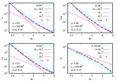
Figure 14: Dependence of the four quantities $\xi_{x}$, $\xi_{\rm CM}$, $\xi_{E}$ and $L_{2}$ on disorder $W$ in a double logarithmic scale for $U_{R}=1$, $U=2$ and $E=0$ (black squares). Furthermore for the cases $\xi_{x}$, $\xi_{\rm CM}$ and $L_{2}$ also the fit $aL_{1}+bL_{1}^{2}$ with $L_{1}=105/W^{2}$ (blue curve), the asymptotic formulas $aL_{1}$ (pink line), $bL_{1}^{2}$ (red line) and the power law fit $CW^{-\gamma}$ (light blue line, shifted by a factor of 2) are shown. For the case $\xi_{E}$ also the fit $a+bL_{1}^{1/3}$ (blue curve), the asymptotic formula $bL_{1}^{1/3}$ (red line) and the power law fit $CW^{-\gamma}$ (light blue line, shifted by a factor of 0.75) are shown. The fit results are for $\xi_{E}$ : $a=-8.0\pm 0.3$, $b=11.2\pm 0.2$, $C=46.2\pm 1.4$, $\gamma=0.95\pm 0.03$, for $\xi_{x}$ : $a=2.97\pm 0.08$, $b=0.052\pm 0.004$, $C=830\pm 60$, $\gamma=2.60\pm 0.07$, for $\xi_{\rm CM}$ : $a=3.08\pm 0.07$, $b=0.104\pm 0.006$, $C=1360\pm 110$, $\gamma=2.85\pm 0.07$, and for $L_{2}$ : $a=0.569\pm 0.008$, $b=0.047\pm 0.001$, $C=610\pm 50$, $\gamma=3.31\pm 0.07$.

In previous numerical works (e. g. song1 ; leadbeater1 ) but also more recently in flach2011 , a lot of effort was devoted to characterize the enhancement effect (or “absence” of it) by a simple power law fit $L_{2}=CW^{-\gamma}$ which typically provides some exponent $\gamma$ somewhat larger than $2$ (behavior for absence of interaction) but still clearly below $4$ (behavior expected if $L_{2}\sim L_{1}^{2}$). As already discussed in frahm5 one must be very careful with such a fit which is not really justified if there are finite size corrections corresponding to a different behavior such as $L_{2}=aL_{1}+bL_{1}^{2}$ resulting actually in $L_{2}\sim W^{-4}$ when taking the formal limit $W\to 0$ or $L_{1}=105/W^{2}\to\infty$. However, in numerical computations such a limit may be difficult to access, especially if the constant $b$ is rather small as compared to $a$, and in order to distinguish between the two scenarios one must carefully analyze the dependence of $L_{2}$ on $W$, especially the curvature in double logarithmic scale.

In Figure 14 we show for $U=2$ and $E=0$ (cases with linear behavior of the enhancement factor in Figures 7 and 12) the dependence of the four quantities $\xi_{x}$, $\xi_{\rm CM}$, $L_{2}$, and $\xi_{E}$ on disorder $W$ in a double logarithmic scale. The case of $\xi_{E}$ is somewhat particular. For the other three quantities we compare the simple power law fit $CW^{-\gamma}$ with the square polynomial fit $aL_{1}+bL_{1}^{2}$ and show for the latter also the asymptotic limits $aL_{1}$ and $bL_{1}^{2}$ for small or large values of $L_{1}$. For all three cases there is a clear and significant non-vanishing curvature and the square polynomial fit works very well with $a\approx 3$ for $\xi_{x}$ and $\xi_{\rm CM}$ and $a\approx 0.6$ for $L_{2}$ while $b\approx 0.05$ for $\xi_{x}$ and $L_{2}$ and $b\approx 0.1$ for $\xi_{\rm CM}$ also confirming the observations of Figure 13 (see caption of Figure 14 for precise fit results).

The overall power law fit for these cases provide exponents $\gamma=2.61$ for $\xi_{x}$, $\gamma=2.86$ for $\xi_{\rm CM}$ and $\gamma=3.31$ for $L_{2}$. At first sight these fits appear indeed rather close to the data points (in double logarithmic scale) but the deviations are systematic and not random. Furthermore, when the lines obtained by power law fits are slightly shifted up one sees very clearly that the deviations are due to the non-vanishing curvature of the data. However, if the interval of available data values of $W$ is reduced (e. g. for $2\leq W\leq 5$) or if the data for small $W$ are simply invalid (for example when using finite size scaling for too small system sizes in the raw data) one may get the wrong impression that the simple power law appears justified.

For $\xi_{E}$ the dependence on $W$ is quite different. Motivated by the fit result of Figure 6 with $\gamma_{3}=0.35$ we use here the fit $\xi_{E}=a+bL_{1}^{1/3}$ which gives $a=-7.9$ and $b=11.2$ and is very accurate while the power law fit $\xi_{E}\propto W^{-\gamma}$ gives the exponent $\gamma=0.94$ corresponding $\xi_{E}\sim L_{1}^{0.47}$ and shows quite significant deviations. In all four cases one sees that the slope of the simple power law fit is quite different from the slope of the asymptotic behavior for large $L_{1}$ and that the former is not sufficiently accurate for the full interval of considered disorder values.

Even tough the square polynomial fit in $L_{1}$ (for the first three quantities) does not apply to all interaction values according to Figures 7 and 12 the analysis shown in Figure 14 illustrates clearly the problems and limitations associated to the simple power law fit for the disorder dependence of the different types of two-particle localization lengths.

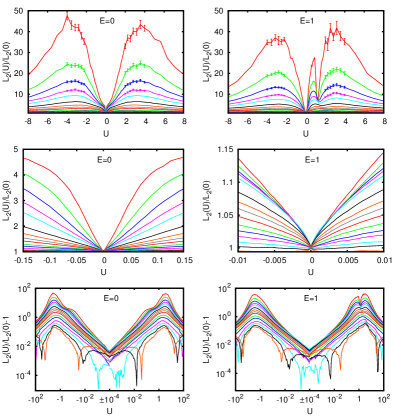
Figure 15: Dependence of $L_{2}(U)/L_{2}(0)$ on $U$ for $E=0$ (left panels) and $E=1$ (right panels) and the disorder values $W$ used in Figure 11 with $W=0.5$ for the top red curves and increasing values of $W$ corresponding to decreasing curves. Here $L_{2}(U)$ represents the infinite size localization length obtained by finite size scaling for the interaction strength $U$. Top panels show the curves on normal scale for $-8\leq U\leq 8$ with error bars for data in the range $2\leq|U|\leq 4$ and top four curves. Error bars for other curves are below line size. Center panels show the zoomed range $-0.15\leq U\leq 0.15$ ($-0.01\leq U\leq 0.01$) for $E=0$ ($E=1$) on normal scale. Bottom panels show $L_{2}(U)/L_{2}(0)-1$ in logarithmic scale versus $U$ for $10^{-4}\leq|U|\leq 10^{2}$ in a logarithmic scale with sign corresponding to $U\leq-10^{-4}$ for the left half and $U\geq 10^{-4}$ for the right half of the $U$-axis.

We also studied the dependence of the infinite size localization length $L_{2}(U)$ on the interaction strength $U$ (with $L_{2}(U)$ obtained by finite size scaling and not to be confused with the finite size quantity $L_{2}(N)$ used in Figures 11 and 18). Exploiting the optimization of the Green function expression (12) we computed simultaneously $L_{2}(U)$ with nearly no additional effort for a large number of interaction values which are the 7 reference values used in Figure 12, 121 values in the range $10^{-4}\leq U\leq 10^{2}$ and further 121 values in the range $-10^{2}\leq U\leq-10^{-4}$ giving 249 different values for $U$. The latter two groups are uniformly distributed in logarithmic scale for $|U|$, i. e. with a constant factor $10^{1/20}\approx 1.122$ between two neighbor values of $|U|$. According to the discussion at the end of Section 2, we used the optimized expression (12) for the most difficult cases of smallest disorder and $N\leq 20L_{1}$ while for some less difficult cases for large disorder and $N>20L_{1}$ we directly used the more expensive matrix inversion in (11) for reasons of numerical stability.

The dependence of $L_{2}(U)/L_{2}(0)$ on $U$ for the two energies $E=0$ and $E=1$ is shown in Figure 15. The top panels show this quantity in normal scale for $-8\leq U\leq 8$ and with error bars for the top 4 curves (for smallest values of $W$) in the ranges $2\leq|U|\leq 4$ close to the maxima. Since the behavior for very small interaction values appears to be very particular, we also show (in center panels) the zoomed region $|U|\leq 0.15$ ($|U|\leq 0.01$) for $E=0$ ($E=1$). In bottom panels the quantity $L_{2}(U)/L_{2}(0)-1$ is shown in logarithmic scale versus a logarithmic scale with sign for $U$, i. e. the two regions of positive and negative values of $U$ are both presented in logarithmic scale of $|U|$ and they are joined together at $U=\pm 10^{-4}$.

For $E=0$ the first observation is that the dependence of $L_{2}(U)/L_{2}(0)$ on $U$ is an even function in average but that there are small statistical fluctuations within the margin of statistical error that do not respect this symmetry. This behavior is easily understood theoretically since a change of sign of $U$ can be taken into account by replacing the disorder potential according to $V(x)\to-V(x)$, which corresponds to a different statistical sample, and by the transformation $\psi(x_{1},x_{2})\to(-1)^{x_{1}+x_{2}}\psi(x_{1},x_{2})$ which accounts for the change of sign of the hopping matrix element in (1). Furthermore we observe roughly a linear behavior $\sim|U|$ for small $|U|$ and a decay $\sim|U|^{-1}$ for large $|U|$, which is also somehow suggested by the analytic form of the projected Green function (11) in terms of $U$. We therefore confirm our above observation of Figure 10 that the enhancement effect indeed vanishes for $U\gg 1$ not only for $\xi_{x}$, $\xi_{\rm CM}$ and $\xi_{E}$ but also for $L_{2}$ in agreement with the theoretical predictions of ponomarev1 . The curves are maximal in the region $3\leq|U|\leq 4$, at least for the smallest disorder values (top curves) where the maxima are rather clearly visible. There is a tendency that the maximum positions are slightly moving closer to 0 with increasing disorder. The curves increase from $U=0$ to $|U|\approx 0.1$ quite abruptly with values up to $4$-$5$ for the two smallest disorder values. Actually, the double logarithmic scale of bottom panels shows that there are two different linear regimes for small and medium values with two different slopes. For example for $W=0.5$ the fit $L_{2}(U)/L_{2}(0)=a+b|U|$ in the range $|U|\leq 0.1$ provides $a=0.999\pm 0.003$ and $b=35.7\pm 0.2$ while for larger values $0.8\leq|U|\leq 2$ it gives $a=-3.9\pm 0.4$ and $b=18.1\pm 0.3$ corresponding to roughly a factor of two between the two slopes.

For the other energy $E=1$ one does not expect a symmetry between positive and negative values of $U$ and indeed for positive $U$ there is for small disorder values (top curves) a well pronounced local minimum close to $U\approx 1.2$ which is completely absent for negative values of $U$. Motivated by this finding we have also computed a few additional data points for $1<U<1.5$ and $E=1$ for the IPR quantities. These data points were included in Figure 10 where one can see a slight reduction for a similar $U$ value and smallest disorder but this reduction is also of the order of statistical fluctuations. The three IPR quantities do not show the clear local minimum as the Green function localization length $L_{2}$ but the region of maximum values in Figure 10 for $E=1$ is quite large which is coherent with a scenario that the minimum is somehow smoothed out for the IPR quantities. Apart from this the overall form of the curves in Figure 10 for $E=1$, with an enlarged $U$-regime for high values, is coherent with Figure 15. Furthermore in Figure 15 for $E=1$ the behavior $\sim|U|^{-1}$ for large $|U|$ appears to be similar as to $E=0$. For the region $|U|\leq 0.01$ there is for $E=1$ a slight sublinear behavior and the power law fit $L_{2}(U)/L_{2}(0)-1=C|U|^{\gamma}$ provides for $0<U\leq 0.01$ and $W=0.5$ the values $C=6.62\pm 0.10$ and $\gamma=0.830\pm 0.003$ and for $-0.01\geq U>0$ the values $C=5.65\pm 0.10$ and $\gamma=0.812\pm 0.003$. The differences between the two cases are due to a slight asymmetry. Using all positive and negative values in the range $|U|\leq 0.01$ for the fit one obtains $C=6.1\pm 0.2$ and $\gamma=0.822\pm 0.006$.

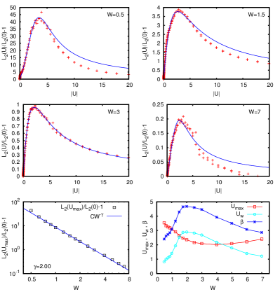
Figure 16: Top and center panels: Comparison of the interaction dependence of $L_{2}(U)/L_{2}(0)-1$ (same data as in Figure 15) with the fit (24) for $E=0$ and the disorder values $W=0.5,\,1.5,\,3,\,7$. Note that due to the symmetry of $F(U)$ data points for $U<0$ are mapped to the positive $U$-axis. Bottom left: Dependence of $F_{\rm max}=L_{2}(U_{\rm max})/L_{2}(0)-1$ on the disorder strength $W$ (black squares). The full blue line shows the power law fit $L_{2}(U_{\rm max})/L_{2}(0)-1=C\,W^{-\gamma}$ with $C=8.66\pm 0.10$ and $\gamma=1,999\pm 0.017$. Bottom right: Dependence of the fit parameters $U_{\rm max}$ (red squares), $U_{w}$ (light blue circles) and the quantity $\beta$ (blue stars) given by (25) on the disorder strength $W$.

Since for the case $E=0$ and each value of $W$ the curve $L_{2}(U)/L_{2}(0)-1$ is an even function in $U$ and due to the above observation that it obeys the limits $L_{2}(U)/L_{2}(0)-1\sim|U|$ for $|U|\ll 1$ and $L_{2}(U)/L_{2}(0)-1\sim|U|^{-1}$ for $|U|\gg 1$ one can try (for each disorder value $W$) the fit

$$L_{2}(U)/L_{2}(0)-1=F(U)$$ (23)

with

$$F(U)=F_{\rm max}\,\frac{|U|\,U_{w}/U_{\rm max}}{(1-|U|/U_{\rm max})^{2}+|U|\,U_{w}/U_{\rm max}}$$ (24)

being a rational function in $|U|$ and where the positive quantities $F_{\rm max}$, $U_{\rm max}$ and $U_{w}$ represent the three (disorder dependent) fit parameters. One verifies directly that this function has its maxima at $U=\pm U_{\rm max}$ with the value $F(\pm U_{\rm max})=F_{\rm max}$. The quantity $U_{w}$ represents somehow the (square of the) decay width around the maxima for the dimensionless quantity $|U|/U_{\rm max}$. Furthermore, the ansatz (24) obeys both limits for small and large $|U|$-values, and the duality relation $F(U)=F(U_{\rm max}^{2}/U)$. Let us introduce the quantity $\beta>1$ such that $F(\beta U_{\rm max})=F(\beta^{-1}U_{\rm max})=F(U_{\rm max})/2$, i. e. : $\beta^{-1}U_{\rm max}$ and $\beta U_{\rm max}$ are the two values on the positive $U$-axis where the value of $F(U)$ is reduced by a factor $1/2$ with respect to its maximum value. From (24) one finds that $\beta$ is related to $U_{w}$ by:

$$\beta=1+U_{w}/2+\sqrt{U_{w}+U_{w}^{2}/4}\ .$$ (25)

Increasing values of $U_{w}$ and $\beta$ indicate a larger width around the maxima of $F(U)$. Performing the fit with the ansatz (24), using the data of Figure 15, we determined for each disorder value the three parameters $F_{\rm max}$, $U_{\rm max}$, $U_{w}$, and via (25) the related quantity $\beta$. The non-linear fit is a bit tricky and we used stronger weights for larger data values closer to the maximum. The particular region $U<0.1$ and the limit $U\gg 1$ are not very precisely captured but the data close to the maximum are quite accurately represented by the fit as can be seen in Figure 16. Furthermore, the bottom panels of Figure 16 show the disorder dependence of the fit parameters. The quantity $F_{\rm max}=L_{2}(U_{\rm max})/L_{2}(0)-1$ obeys a nearly perfect power law $L_{2}(U_{\rm max})/L_{2}(0)-1\approx 8.7\,W^{-2.00}$ and using the behavior $L_{2}(0)\approx 0.56\,L_{1}^{1.02}\approx 59\,W^{-2.04}$ (see Figure 13) we find the expression $L_{2}(U_{\rm max})\approx 59\,W^{-2.04}+513\,W^{-4.04}$ which is indeed very accurate. A more direct fit with integer exponents gives a very similar expression: $L_{2}(U_{\rm max})\approx 54\,W^{-2}+586\,W^{-4}$. The finite size correction $\sim L_{1}\sim W^{-2}$ is quite important and a (too) simple power law fit without this correction would provide $L_{2}(U_{\rm max})\approx 622\,W^{-3.49}$ with rather strong systematic deviations due to a non-vanishing curvature (in double logarithmic scale) in a similar way as in Figure 14 for $L_{2}(U=2)$. The values of $U_{\rm max}$ and the width parameters $U_{w}$ or $\beta$ are not constant with respect to the disorder strength and for smaller values of $W$ close to $0.5$ the width of the curve $F(U)$ around its maxima is considerably reduced. This point explains that $L_{2}(U)/L_{1}$ is below the behavior $a+bL_{1}$ for $U\leq 1.0$ in the left panel of Figure 12 since for smaller values of $W$ (larger values of $L_{1}$) the interaction values $U\leq 1$ are already out of resonance with respect to their optimal value $U_{\rm max}$. However, for $U=2$, which is closer to $U_{\rm max}$, the behavior $L_{2}(U)/L_{1}\approx a+b\,L_{1}$ is clearly valid for all considered disorder values $W\geq 0.5$.

Another interesting point concerns the duality with respect to $U\to\sqrt{24}/U$ predicted in waintal1a . The fit function $F(U)$ verifies such a duality relation provided $U_{\rm max}^{2}=\sqrt{24}$ corresponding to $U_{\rm max}\approx 2.2$ which is approximately valid for $W\geq 2$ according to Figure 16. Therefore we can approximately confirm this duality for such disorder values but not for the region $0.5\leq W<2$. However, in general we have a modified duality relation $U\to U_{\rm max}^{2}/U$ with $U_{\rm max}$ depending on $W$ according to Figure 16. Actually a more general duality relation $U\to{\rm const.}/U$ was suggested in ponomarev1 . Furthermore, the duality relation does not precisely extend to the extreme regions $|U|\leq 0.1$ or $|U|\geq 50$.

We have also applied the fit (24) to the data of Figure 10 for $E=0$ concerning the interaction dependence of the three IPR quantities $\xi_{x}$, $\xi_{\rm CM}$ and $\xi_{E}$. Due to less available data points the fits are more difficult. We mention only that we find the following power laws : $\xi_{E}(U_{\rm max})-1\sim W^{-0.88}$, $\xi_{x}(U_{\rm max})-\xi_{x}(0)\sim W^{-3.24}$, and $\xi_{\rm CM}(U_{\rm max})-\xi_{\rm CM}(0)\sim W^{-3.40}$. Here the last two exponents for $\xi_{x}$ and $\xi_{\rm CM}$ are quite different from $-4$ found for $L_{2}$. To understand this we first note that the exponents of the reference values at $U=0$ of $\xi_{x}(0)\sim W^{-1.33}$ and $\xi_{\rm CM}(0)\sim W^{-1.52}$ are different from $-2$ (see the fits for $E=0$ and $U=0$ of Figure 13). Furthermore for $\xi_{x}$ and $\xi_{\rm CM}$ the maximum position $U_{\rm max}$ moves to quite small values well below $1$ for larger disorder values which changes the functional dependence of $\xi_{x,{\rm CM}}(U_{\rm max})$ on $W$ since at small $U$ and large $W$ the two IPR quantities are relatively enhanced as compared to $L_{2}$.

In summary, in this section we have established the behavior $L_{2}=aL_{1}+bL_{1}^{2}$ for optimal interaction values, clarified that a simple power law fit $L_{2}\sim W^{-\gamma}$ is not well justified and how to understand exponents $\gamma$ below $4$ obtained by such fits. We have also obtained new and interesting results for the precise interaction dependence, such as a special regime for very small interaction values or a well pronounced local minimum at a finite value $U>0$ for $E=1$. Furthermore the discussion in Appendix C shows that the finite size scaling procedure requires a careful treatment of the condition $N>L_{1}$ on used data points, implying that previous results song1 ; leadbeater1 obtained for $N\leq 250$ and $W\leq 1.5$ are simply invalid. Also the use of constant offsets (independent of sample size) for the reference positions when measuring the localization length by the exponential decay of the Green function must be avoided since they imply a non-trivial transformation on the raw-data tainting completely the results of the scaling procedure.

6 Internal eigenfunction structure inside the localization domain

A typical TIP localized eigenstate of length $L_{2}$ in the center of mass coordinate and width $L_{1}$ in the relative coordinate extends to a domain of potential $L_{1}L_{2}\sim L_{1}^{3}$ non-interacting product eigenstates in energy representation. Our results of Section 4 clearly indicate that the number of such states that really contribute to a TIP eigenstate, which is roughly $\xi_{E}$ the IPR in energy representation, is far below the size of this domain providing therefore a non-trivial internal eigenfunction structure.

Theoretically it was first expected that only non-interacting product eigenstates in an energy interval $\sim\Gamma$ are mixed where $\Gamma$ is the Breit-Wigner width implying the estimate $\xi_{E}\sim L_{1}L_{2}\Gamma/B_{W}$ where $B_{W}\sim 1$ is the total band width of two-particle energies jacquod1 ; fyodorov1 ; frahm2 . The first scenario proposed in the initial work dlstip assumed that a typical interaction matrix element (for $U_{R}=1$),

$$U_{\nu_{1}\nu_{2},\,\nu_{3}\nu_{4}}=U\sum_{x}\phi_{\nu_{1}}(x)\,\phi_{\nu_{2}}(x)\,\phi_{\nu_{3}}(x)\,\phi_{\nu_{4}(x)},$$ (26)

behaves as $\sim U/L_{1}^{3/2}$ if all one-particle wave functions are localized at roughly the same position with amplitudes $\sim L_{1}^{-1/2}$ and random phases inside the localization domain providing an additional factor $\sim L_{1}^{1/2}$ due to the sum of $L_{1}$ random numbers. Using this assumption the Breit Wigner width is estimated as $\Gamma\sim U^{2}/L_{1}$ (assuming a unit coupling element $t=1$ in the initial Anderson model) leading to the estimates $L_{2}\sim U^{2}L_{1}^{2}$ and $\xi_{E}\sim U^{4}L_{1}^{2}$ jacquod1 ; fyodorov1 ; frahm2 . These two estimates disagree both with the numerical results of Figures 10 and 15 concerning the interaction dependence and the expression for $\xi_{E}$ also disagrees strongly for the dependence on $L_{1}$ with the results of Figures 6 (lowest curve in bottom right panel) or 7-9 (bottom panels) predicting a power law $\xi_{E}\approx a+bL_{1}^{\gamma}$ with constant term and $\gamma$ clearly below 1 (e. g. $\gamma=1/3$ for $U=2$, $E=0$, $U_{R}=1$).

The main reason of this discrepancy is that the phases of the localized one-particle wave functions are (for small disorder) quite strongly correlated due a plane wave structure with rather well defined momenta. Therefore the interaction matrix elements strongly fluctuate with maximum values $\sim U/L_{1}$ due to an approximate momentum conservation with uncertainty $\sim 1/L_{1}$ and much smaller values for non-conserved momenta ponomarev1 .

The analytical calculation (to all orders in $U$) of the Breit-Wigner width for the case of vanishing disorder jacquod2 and the extension in frahm5 provide indeed a modified dependence $\Gamma\sim c(U)/L_{1}$ with $c(U)\sim|U|$ for $|U|\lesssim 1$ resulting in $L_{2}\sim c(U)L_{1}^{2}$. This behavior is closer to the numerical results but at first sight the modification of the above estimate of $\xi_{E}$ would provide $\xi_{E}\sim c(U)^{2}L_{1}^{2}\sim U^{2}L_{1}^{2}$ which still clearly contradicts our numerical data.

We attribute this to the fact that the Breit-Wigner width actually depends strongly on the quasi-momenta $k_{\nu_{1}}$ and $k_{\nu_{2}}$ of the initial non-interacting product eigenstate for which it is computed as can be clearly seen in the calculations of jacquod2 ; frahm5 , i. e. the estimate $\Gamma\sim c(U)/L_{1}$ corresponds to the average $\Gamma=\langle\Gamma^{(1)}_{\nu_{1}\nu_{2}}\rangle_{\nu_{1},\nu_{2}}$ with respect to these momenta with $\Gamma^{(1)}_{\nu_{1}\nu_{2}}$ for example given by equation (22) of frahm5 . The variations of $\Gamma^{(1)}_{\nu_{1}\nu_{2}}$ are also visible in Figure 4 due to the non-uniform structure of the energy line $E\approx\epsilon_{\nu_{1}}+\epsilon_{\nu_{2}}$. When determining $L_{2}\sim\Gamma L_{1}^{3}$ the average Breit-Wigner width seems to produce rather reasonable dependencies of $L_{2}$ on $U$ and $L_{1}$ (even though a more accurate theory is still lacking) but for $\xi_{E}$, requiring an harmonic average $\xi_{E}\sim L_{2}L_{1}\langle(B_{W}/\Gamma^{(1)}_{\nu_{1}\nu_{2}})\rangle_{\nu_{1},\nu_{2}}^{-1}$, the strong fluctuations of $\Gamma^{(1)}_{\nu_{1}\nu_{2}}$ with possible quite small values will considerably reduce $\xi_{E}$ thus explaining the lower exponents $\gamma$ clearly below unity.

It is interesting to note that for the random matrix ensembles proposed by Ponomarev et al. ponomarev1 , which are modelized by carefully taking into account the strong fluctuations of the interaction matrix elements as well as the approximate momentum conservation for best coupled states, the power law $\xi_{E}\sim L_{1}^{\gamma_{\rm ipr}}$ is expected with typical values of $\gamma_{\rm ipr}$ clearly below unity according to Figure 1 of ponomarev1 for at least one variant of the modified random matrix ensembles studied in ponomarev1 .

The physical picture of strongly fluctuating interaction coupling matrix elements and Breit-Wigner widths depending on the initial state corresponds to the situation where among $\sim L_{1}L_{2}$ potential non-interacting product eigenstates in the localization domain one has to select first states fulfilling the condition

$$|E-\epsilon_{\nu_{1}}-\epsilon_{\nu_{2}}-U_{\rm diag}+\Gamma^{(0)}_{\nu_{1}\nu_{2}}/2|\lesssim\Gamma^{(1)}_{\nu_{1}\nu_{2}}$$ (27)

where $U_{\rm diag}=<\!\phi_{\nu_{1}}\,\phi_{\nu_{2}}|\hat{U}|\phi_{\nu_{1}}\,\phi_{\nu_{2}}\!>\,\,\sim U/L_{1}$ is a diagonal interaction matrix element with the same sign as $U$ but with considerable fluctuations. $\Gamma^{(0)}_{\nu_{1}\nu_{2}}$ is the real part of the self-energy while the Breit-Wigner width $\Gamma^{(1)}_{\nu_{1}\nu_{2}}$ is the imaginary part as given in equations (14) and (15) of frahm5 . The approximate momentum conservation implies an additional selection criterion

$$|k_{\nu_{1}}+k_{\nu_{2}}-k_{\nu_{3}}-k_{\nu_{4}}|\lesssim 1/L_{1}$$ (28)

(or similar with modified signs for the different momenta) for two strongly coupled non-interacting product eigenstates ponomarev1 . For the energy $E=0$ at the band center, with an approximate Fermi surface with linear borders in momentum space (see left panels of Figure 3), both selection criteria (27) and (28) seem to select rather similar states but the situation is more complicated due to the shifts from $U_{\rm diag}$ and $\Gamma^{(0)}_{\nu_{1}\nu_{2}}/2$ and of course due to the strong fluctuations of $\Gamma^{(1)}_{\nu_{1}\nu_{2}}$. For the energy $E=1$ outside the band center the form of the approximate Fermi surface is different (see right panels of Figure 3) and the overlap for both criteria appears to be somewhat reduced. However, this effect does not seem to reduce $\xi_{E}$ for $E=1$ if compared to $E=0$ according to results shown in Figures 7-10. Combining the effects of the strong fluctuations of the Breit-Wigner width, the shifts due to the diagonal interaction matrix elements and the real part of the self-energy, and the additional approximate momentum conservation it finally appears that typical TIP eigenstates select only a rather modest number $\sim\xi_{E}\sim L_{1}^{\gamma}\ll L_{1}^{2}$ of non-interacting product eigenstates with $\gamma<1$. However, due to a complicated spatial distributions of such states and their large individual values of $\Gamma^{(1)}_{\nu_{1}\nu_{2}}$ they still produce an overall localization length $L_{2}\sim L_{1}^{2}$ (for certain optimal interaction values).

7 Discussion

In this work numerous new numerical results for various quantities characterizing the localization and other properties of TIP eigenfunctions for the one-dimensional Anderson model have been obtained. The dependence of the three types of localization lengths $\xi_{x}$, $\xi_{\rm CM}$ and $L_{2}$ on $L_{1}$ can be well fitted by $aL_{1}+bL_{1}^{\gamma}$ for a large range of disorder and with $\gamma\approx 2$ for a considerable interval of optimal interaction values.

However, for the interaction dependence the behavior $L_{2}/L_{1}\approx c(U)L_{1}+$const. as suggested in vonoppen ; jacquod2 ; frahm5 with various propositions for the coefficient $c(U)$ is not completely confirmed by our new results for the full interval of considered disorder values. In the band center $E=0$ the fit (24) of the quantity $L_{2}(U)/L_{2}(0)-1$ (see Figure 15) provides for each disorder value roughly a similar form with an approximate behavior $\sim|U|$ ($\sim|U|^{-1}$) for $|U|\ll 1$ ($|U|\gg 1$) and the maximal amplitude scales very precisely as $L_{2}(U_{\rm max})/L_{2}(0)-1\sim L_{1}$. However, the maximum position $U_{\rm max}$ and the effective width parameter of (24) depend on disorder according to Figure 16. In particular the width of these curves decreases considerably for the smallest disorder values thus explaining the sublinear behavior of $L_{2}(U)/L_{1}$ in $L_{1}$ for interaction values not sufficiently close to $U_{\rm max}$. Furthermore, the duality with respect to $U\to{\rm const.}/U$ predicted in ponomarev1 ; waintal1a is roughly confirmed by our data.

The new claims of flach2011 ; flach2014 concerning a strongly reduced TIP enhancement are based on numerical data for limited parameters in system size ($N\leq 234$) and disorder ($W\geq 2$) for TIP eigenfunctions and without use of finite size scaling. Furthermore in flach2011 the oversimplified power law fit without finite size correction was used (see our above discussion of Figure 14). Our numerical results obtained for very large system sizes and by careful finite size scaling, especially with respect to the condition $N>L_{1}$ neglected in previous work song1 ; leadbeater1 , refute very clearly the new claims of flach2011 ; flach2014 .

We have also considered the inverse participation ratio in energy representation (of non-interacting product eigenstates) which clearly demonstrates the interaction induced delocalization by values $\xi_{E}\gg 1$ such as $\xi_{E}\approx 222$ or $\xi_{E}\approx 168$ for the two example eigenstates with $N=5000$ shown in Figure 1. This quantity obeys a different dependence on $L_{1}$ as $\xi_{E}\approx a+bL_{1}^{\gamma}$ with $\gamma\approx 1/3$ (for $U=2$, $E=0$ and the Hubbard interaction case) and somewhat larger values with $0.6\leq\gamma\leq 0.9$ for the interaction range $U_{R}=5$. This behavior is indeed unexpected if compared to the early results based on the random band matrix model with preferential basis that suggested $\xi_{E}\sim L_{1}^{2}$ jacquod1 ; fyodorov1 ; frahm2 . As explained in Section 6 this estimate was obtained from an incorrect hypothesis about uncorrelated phases inside the localization domain of non-interacting one-particle eigenfunctions. An accurate quantitative analytical theory for this quantity, beyond the random band matrix model of jacquod1 ; fyodorov1 ; frahm2 , is still missing but qualitatively it seems that the scaling $\xi_{E}\sim L_{1}^{\gamma}$ with $\gamma<1$ is related to very strong fluctuations of the Breit-Wigner width depending strongly on the unperturbed initial state for which it is computed.

We have also established a particular regime of rather strong enhancement for quite low interaction values and obtained new very interesting results for an energy $E=1$ outside the band center such as a strong local minimum in the interaction dependence of $L_{2}(U)/L_{2}(0)$ at the value $U\approx 1.2$ (see Figure 15). Also for these new results a precise analytical theory is still missing.

The very efficient numerical methods used in this work allowed to considerably extend the range of parameters in system size, low disorder values, very small and large interaction values for which results for various quantities were obtained. These methods are potentially also applicable for TIP in higher dimensions (see e. g. ortuno1 ) even though the efficiency gain will be more moderate, especially for the computation of the projected Green function $\bar{G}_{0}$ at vanishing interaction which is the basic step for both methods.

The author thanks Dima Shepelyansky for numerous fruitful discussions and Gabriel Lemarié for his insight on the numerical scaling procedure. The author is particularly grateful for the access to the HPC resources of CALMIP (Toulouse) under the allocation 2015-P0110 during this work.

Appendix A Computation of the scaling curve

In this appendix we provide some details on the explicit procedure we used to compute the scaling curve and to determine the infinite size localization lengths for the TIP problem. Our approach is somewhat different from the scaling fit procedure given in mackinnon2 and in particular it also allows to take into account (and to compute) the statistical errors of the finite (infinite) size localization lengths in a quite simple way.

Let us assume that we have numerical raw data of finite size localization lengths $\xi_{j}(N)$ dependent on system size $N$ and on an index $j=0,\,1,\,2,\,\ldots$ representing several data sets for different disorder values (with increasing values of $j$ corresponding to decreasing of values of the disorder strength). The “localization length” $\xi$ may correspond to one of the three IPR-localization lengths $\xi_{x}$, $\xi_{\rm CM}$ or $\xi_{E}$ or to the Green function localization length $L_{2}$. Typically these localization lengths are obtained by some kind of averaging procedure which also provides data for the statistical errors $\delta\xi_{j}(N)$. Furthermore we assume that all data sets correspond to the same values of other physical parameters such as energy, interaction strength, interaction range, boson- or fermion case etc.

Assuming the validity of one-parameter scaling we need to find a universal scaling function $f(x)$ and “infinite size localization lengths” $\xi_{j}(\infty)$ for each data set such that the data are well fitted by mackinnon1 ; mackinnon2 ; kramer1 :

$$\frac{\xi_{j}(N)}{N}=f\left(\frac{\xi_{j}(\infty)}{N}\right)\ .$$ (29)

The scaling function has the obvious limit $f(x)=x$ for $x\ll 1$. Furthermore it turns out that $f(x)$ is monotonically increasing and tends to some limit $f_{\infty}$ for $x\to\infty$ corresponding to the behavior $\xi_{j}(N)\approx f_{\infty}\,N\sim N$ in the regime $N\ll\xi_{j}(\infty)$. We mention that for the TIP problem this point requires to exclude data with $N<L_{1}$ where $L_{1}=105/W^{2}$ is the one-particle localization length and as discussed in Appendix C the validity of one-parameter scaling indeed requires $N$ to be larger than all other length scales mackinnon2 ; kramer1 , especially $L_{1}$ which plays in our case somehow the role of the mean free path.

Usually, to perform the scaling procedure in a graphical way one draws for each data set the logarithm of $\xi_{j}(N)/N$ versus the logarithm of $1/N$ and applies a horizontal shift on each curve such that all data fall on the same universal scaling curve where the horizontal shift provides the (logarithm of the) infinite size localization length $\xi_{j}(\infty)$ (see Figures 6 and 11). Below we describe an explicit, efficient and reliable implementation of this procedure suitable to treat automatically a large amount of different data sets for many different cases and to obtain the best possible accuracy together with an estimate of the statistical error of $\xi_{j}(\infty)$.

Explicitely, let us define for each available value of $N=N_{l}$ and disorder index $j$ : $x_{j,l}=1/N_{l}$ and $y_{j,l}=\xi_{j}(N_{l})/N_{l}$. Furthermore, let $y_{j,{\rm max}}=\max_{l}\,(y_{j,l})$, $y_{j,{\rm min}}=\min_{l}\,(y_{j,l})$, and $\bar{x}_{j}$ the $x$-value associated to $y_{j,{\rm max}}$. First we remove all data points with $x_{j,l}>\bar{x}_{j}$ and $y_{j,l}<y_{j,{\rm max}}$ corresponding to data on the right side of (and below) the maximum in $y$ which are problematic since they clearly violate the monotonicity between $x$ and $y$ and produce a partly double valued curve. Such data points are either in the problematic flat regime of the scaling curve for $x\gg 1$ or indicate that for them the one-parameter scaling hypothesis is not verified, e. g. if the ratio $N_{l}/L_{1}$ is not yet sufficiently large (this may especially happen for the cases of $\xi_{x}$ and $\xi_{\rm CM}$). Let us denote by $h(y)$ the inverse of the scaling function $f(x)$ such that $h(y)=x$ is equivalent to $y=f(x)$. Furthermore we translate the known statistical errors $\delta y_{j,l}=\delta\xi_{j}(N_{l})/N_{l}$ for $y_{j,l}$ to errors $\delta x_{j,l}\approx(\Delta x/\Delta y)\,\delta y_{j,l}$ for $x_{j,l}$ where $\Delta x/\Delta y$ is the local slope of the $(y,x)$ curve (at given value $j$) obtained from the neighbor values of $x$ and $y$ on this curve.

Let us assume that we have for a given value of $j$ already determined the inverse scaling functions $h_{i}(y)$ for $i=0,\,1,\,\ldots,\,j-1$ of the previous data sets (see below for details on this). Then the horizontal shift for the data set $j$ can be determined from the average :

$$\ln[\xi_{j}(\infty)]=C\sum_{i=0}^{j-1}\sum_{l\in S_{i}}w_{j,l}\Bigl{(}\ln[h_{i}(y_{j,l})]-\ln(x_{j,l})\Bigr{)}$$ (30)

with the weights $w_{j,l}=(\delta x_{j,l}/x_{j,l})^{-2}$ and the $l$-sum runs over the set $S_{i}$ containing the values of $l$ such that $y_{i,{\rm min}}\leq y_{j,l}\leq y_{i,{\rm max}}$ because $h_{i}(y)$ is not defined for $y>y_{i,{\rm max}}$ or $y<y_{i,{\rm min}}$. The normalization constant $C$ is determined by the inverse sum of the weights over exactly the same contributions in $i$ and $l$. It is easy to verify that this average corresponds to the least square (one-parameter) fit to minimize the horizontal differences in logarithmic scale of the data curve $j$ to the previous already rescaled curves and using the weights $w_{j,l}$. We note that the procedure of mackinnon2 is quite different since it performs a single fit to determine simultaneously all shifts and furthermore it corresponds to the choice of constant weights. Our choice of weights proportional to the inverse square of the statistical errors of $\ln(x_{j,l})$ is quite standard in the context of least square fits and has the advantage that it automatically takes into account the quality of individual data points. In particular in the flat region of the scaling curve the slope $\Delta x/\Delta y$ is typically quite large thus strongly increasing the errors in $x$ and reducing the weight of less reliable data in this problematic region.

We also compute the statistical error $\delta\varepsilon_{j}$ of the average (30) in the standard way as the square root of the averaged squared deviations of the shifts multiplied by $\sim 1/\sqrt{d-1}$ where $d$ is the number of independent data points used for the fit. We have chosen for $d$ the number of different $l$ values which contribute in the sum of (30) even though this sum runs over more terms due to the sum over $i$ of previous scaling curves which is only an artificial effect of the notation. In particular for the case where only one single data point ($d=1$) contribute this implies an “infinite error”, a case which actually appears in Figure 19. Furthermore, for $j>0$ we increase the error by $\delta\varepsilon_{j}\to\sqrt{\delta\varepsilon_{j}^{2}+\delta\varepsilon_{j-1}^{2}}$ using the error $\delta\varepsilon_{j-1}$ of the previous data set $j-1$. This takes into account that also the previous inverse scaling curves $h_{i}(y)$ are subject to an error of their respective scaling factors with the most important contribution arising form the last previous data set $j-1$. Finally the error of $\xi_{j}(\infty)$ is obtained as $\delta\xi_{j}(\infty)=\delta\varepsilon_{j}\,\xi_{j}(\infty)$.

Once $\xi_{j}(\infty)$ is known we replace $x_{j,l}\to\xi_{j}(\infty)\,x_{j,l}$ and determine the next piece $h_{j}(x)$ of the inverse scaling function either by linear interpolation [in $\ln(x)$ and $\ln(y)$] or suitable fits of the rescaled discrete data set $j$ (see below).

At the beginning of this procedure at $j=0$, the case with strongest disorder ($W=7$) or smallest localization length ($\xi\approx 1.5-4$), we choose in (30) the limit $h(y)=y$ for $y\ll 1$ as initial scaling curve in order to set approximately the global scale. To improve the precision of the global scale we choose at the end the first data set $j$ containing values with $\xi_{j}(N)\geq 10$, which typically happens at $W=3$ and still provides data points with rather small ratios $\xi_{i}(N)/N\ll 1$, use the fit $\xi_{j}(N)^{-1}=A+B\,N^{-1}$ to determine accurately $\xi_{j}(\infty)=A^{-1}$ for this case, and apply the appropriate correction factor to the other infinite size localization lengths. It turns out that the correction of the global scale due to this improvement is actually quite small and in particular the condition $y\ll 1$ is well fulfilled for the first data set with $W=7$.

This scaling procedure depends on the way the rescaled discrete data points of the set $j$ are translated into a continuous inverse scaling function $h_{j}(y)$ used in the average (30). A simple and quite effective choice is linear interpolation using the logarithmic quantities $X=\ln(x)$ and $Y=\ln(y)$ which already produces very nice scaling curves provided that the raw data are of reasonable quality (good statistical precision of the finite size localization lengths) and that the validity of one-parameter scaling is fulfilled. However, if fluctuations of individual data points are somewhat stronger it is more reasonable to determine $h_{j}(y)$ by a fit such as a polynomial of degree 3 for the dependence of $X$ on $Y$ :

$$X=\ln[h(e^{Y})]=a_{0}+a_{1}\,Y+a_{2}\,Y^{2}+a_{3}\,Y^{3}\ .$$ (31)

The degree 3 appears to be a good compromise between being able to modelize a reasonable curvature and to avoid artificial minima and maxima when using data sets of typically 10-20 points. Even though the fit (31) also provides good scaling curves it can still be improved by incorporating the singularity of $h(y)$ when $y\to f_{\infty}$, with $f_{\infty}$ being the limit of the scaling function $f(x)$ for $x\to\infty$, using a modified fit:

$$X=\ln[h(e^{Y})]=a_{0}+a_{1}\,Y+a_{2}\,Y^{2}+\frac{a_{3}}{F_{\infty}-Y}$$ (32)

with $F_{\infty}=\ln(f_{\infty})$ and $f_{\infty}$ is determined in advance from the last data set (with smallest disorder) by the fit $y^{-1}=f_{\infty}^{-1}+A\,x^{-1}$. We emphasize that during the scaling procedure both fits (31) and (32) are used only on the individual data sets and not on the complete scaling curve obtained so far. Furthermore the value of $F_{\infty}$ is fixed in advance such that both fits are linear in the parameters $a_{j}$, $j=0,\,1,\,2,\,3$ assuring a unique, well defined fit optimum. It turns out that the scaling results are not very sensible to the precise choice of $F_{\infty}$ and are still reasonable if one chooses a rather large value, e. g. $F_{\infty}=\ln(2)$ in case if the automatic determination using the last data set fails for some reason.

One might have the idea to use $F_{\infty}$ as an additional non-linear fit parameter but this works quite badly for the first data sets that do not allow to extract the information concerning the singularity. However, once the scaling procedure using (32) with a fixed value of $F_{\infty}$ is finished we performed such a non-linear fit on all rescaled data to optimize the value $F_{\infty}$ in order to have a full analytical scaling curve for the purpose of illustration (see full blue lines shown in the scaling curves of Figures 6, 11 and panel (a) of Figure 18).

We have also tested modified variants of the scaling procedure where the least square procedure to determine $\xi_{j}(\infty)$ and the linear interpolation or fits to determine $h_{j}(y)$ are not done in logarithmic scale for $X$ and $Y$ but rather in the original variables $x$ and $y$. In this case we have to minimize the weighted sum of squares of the quantity $\alpha_{j}h_{i}(y)-x$ where $\alpha_{j}=1/\xi_{j}(\infty)$ is a (linear) fit parameter. It is straightforward to work out the details of the modified fit procedure, and without going into the details, we mention that it is possible to determine $\xi_{j}(\infty)$ as well as its statistical error $\delta\xi_{j}(\infty)$ by closed formulas. The choice between $y$ and $Y$ does not affect the least square procedure but it modifies the linear interpolation or fits to determine $h_{j}(y)$. In total we have implemented many different variants of the scaling procedure, four for each pairing of $x$ or $X$ with $y$ or $Y$ combined with several cases to obtain $h_{j}(y)$ either by linear interpolation or the two fits (31) and (32). It turns that for good quality raw data all these variants provide coherent results with localization lengths which coincide well within the bounds of the statistical errors obtained from the scaling procedure. However, for bad data (e. g. when trying the very small disorder values $W=0.5$ and $W=0.625$ also for $\xi_{x}$ and $\xi_{\rm CM}$ at $U=2$) the different variants may provide different results or even partly fail. Therefore, the comparison of the different variants gives a good indication on the quality of the data.

Actually, in some cases of “very bad” raw data one may even have a data set $j$ such that all values of $y_{j,l}$ are above all $y$-values of the previous data sets, i. e. where the curves we want to rescale do not even overlap in $y$-direction. In this case one might still try to apply (30) simply by extending the validity of the fits for $h_{i}(y)$ beyond the maximal value of the corresponding curve (“extrapolation mode”) and here the second fit (32) is certainly superior than the polynomial fit (31). Even though this might still provide some estimation of the scaling factors, we did not push this point very far. In particular, all curves and data shown in this work (except for some of the particular and problematic cases shown in Figures 18 and 19) correspond to good quality raw data where all of the above variants of the method as well as the precise fit procedure of mackinnon2 , which we also tested, produce rather precisely the same results (within the margin of errors).

As default method for the scaling procedure we used the variant with both logarithmic variables $X$ and $Y$ and the second fit (32).

Appendix B Two-particle localization lengths at vanishing interaction

In this appendix we discuss our numerical results for the different two-particle localization lengths at vanishing interaction $U=0$ (or very small interaction $U=10^{-5}\approx 0$ for the three IPR quantities). The behavior $\xi_{E}\approx 1$ (lowest curve in bottom panels of Figure 7) is rather precisely confirmed as expected. For the other three localization lengths scales the ratios $\xi_{x}/L_{1}$, $\xi_{\rm CM}/L_{1}$ (lowest curve of top and center panels of Figure 7) and $L_{2}/L_{1}$ (lowest curve of both panels of Figure 12) are of order unity $\sim 1$ but there are still slight variations in the dependence on $L_{1}$ due to the effective average in one-particle energy when measuring these quantities in two-particle space. Also the Green function localization length at $U=0$ contains implicitly such an average as can be seen from the expression (7) for $\bar{G}_{0}$ (see also leadbeater1 for a simplified analytical estimation).

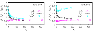
Figure 17: Comparison of the dependence of $L_{2}/L_{1}$, $\xi_{x}/L_{1}$ and $\xi_{\rm CM}/L_{1}$ on $L_{1}$ for $U=0$ and energy $E=0$ ($E=1$) for left (right) panel. The used disorder values $W$ are as in Figure 6 ($\xi_{x}$ and $\xi_{\rm CM}$) or in Figure 11 ($L_{2}$). For $\xi_{x}$ and $\xi_{\rm CM}$ the value $U=10^{-5}\approx 0$ was used.

In Figure 17 these three ratios are shown again as a function of $L_{1}$ but using an increased scale. For $\xi_{x,{\rm CM}}/L_{1}$ we observe a slight decreasing behavior with $L_{1}$, i.e. with strongest values $\approx 2$ for smallest values of $L_{1}$ (largest disorder values) and values slightly below unity for largest values of $L_{1}$ concerning $\xi_{x}/L_{1}$ (both energies) and $\xi_{\rm CM}/L_{1}$ (for $E=0$). For $E=1$ the ratio $\xi_{\rm CM}/L_{1}$ is rather constant with values $\approx 2.2$ and with a very modest local minimum at $L_{1}\approx 25$ and value $\approx 1.9$. To understand this we note that for (nearly) vanishing interaction $\xi_{x,{\rm CM}}$ is computed from a harmonic mean of non-interacting product eigenstates with approximate momenta (or energies) close to the curves (or lines) shown in Figure 3 (or Figure 4). Let $\xi_{1}$ and $\xi_{2}$ be the two IPR values of the two one-particle eigenstates contributing to such a product state. Then we have for the case $\xi_{2}\gg\xi_{1}$: $\xi_{x}=2/(\xi_{1}^{-1}+\xi_{2}^{-1})\approx 2\xi_{1}$ and $\xi_{\rm CM}\approx 2\xi_{2}$. Furthermore, we may assume that roughly $\xi_{j}\sim L_{1}\sin^{2}(k_{j})$ for $|k_{j}|>L_{1}^{-1/3}$ where $k_{1}$ and $k_{2}$ are the approximate momenta of the two one-particle eigenstates. The harmonic average is dominated (reduced) by contributions from small values of $\xi_{j}$, i. e. $k_{j}$ close to $0$, $\pi$, or $2\pi$ (with uncertainty $\sim L_{1}^{-1/3}$) explaining the slight decrease of $\xi_{x,{\rm CM}}/L_{1}$ with increasing $L_{1}$. However for $E=1$ and $\xi_{\rm CM}/L_{1}$ it is more difficult to have product states where both approximate momenta produce simultaneously small values of $\xi_{1}$ and $\xi_{2}$ and here the larger of the two contribute stronger thus explaining the absence of decrease of $\xi_{\rm CM}/L_{1}$ for large $L_{1}$.

$L_{2}/L_{1}$ is for $U=0$ rather constant with values close to $0.5$ for small $L_{1}$ and to $0.65$ for large $L_{1}$. Note that in song1 ; leadbeater1 somewhat larger values closer to $1$ for large $L_{1}$ and $U=0$ where found which is due to a different choice of the parameters used in (21).

The power law fits $\propto L_{1}^{\gamma}$ of the three localization lengths for $U=0$ shown in the bottom panels of Figure 13 provide exponents close to $1$ for both cases of $L_{2}$. For $\xi_{x}$ we have $\gamma=0.66$ ($\gamma=0.70$) and for $\xi_{\rm CM}$ we have $\gamma=0.76$ ($\gamma=0.94$) both for $E=0$ ($E=1$) (see caption of Figure 13 for precise fit results). The reduced exponents for $\xi_{x}$ and $\xi_{\rm CM}$ are due to quite enhanced values at $U=0$ for small $L_{1}$ (stronger $W$) with values close to $2$-$2.5$.

Appendix C Effects of scaling with insufficient system size

The validity of one-parameter scaling theory very clearly requires mackinnon2 ; kramer1 that the system size $N$ is significantly larger than all other typical length scales in the system, especially the mean free path for the usual case of the Anderson model of non-interacting particles. In the case of TIP the one-particle localization length $L_{1}$ is certainly such a length scale and actually plays somehow the role of a mean free path since the dynamics is ballistic for $N<L_{1}$ and diffusive with coherent pair propagation for $L_{1}<N<L_{2}$. Therefore one expects the scaling theory for TIP only to be valid for $N>L_{1}$. Also the physical argumentation in terms of the Thouless scaling block picture imry ; thouless1 shows that it is simply not reasonable to consider values of $N$ below $L_{1}$ in the context of scaling.

The results of song1 ; leadbeater1 obtained by finite size scaling for small disorder values, where $N<L_{1}$ for many or even all data points (for the data sets with lowest disorder) are therefore very problematic in this context. Our numerical results obtained by finite size scaling of the quantity $L_{2}$, defined by (22) and shown in the figures of Section 5, are for small disorder indeed quite different from the results of song1 ; leadbeater1 .

For example for $E=0$, $U=1$ and $W=0.5$ we obtain $L_{2}=3922\pm 102$ while from Figure 2(c) of song1 the corresponding data point provides $L_{2}\approx 1900$ and from Figure 11 of leadbeater1 we get $L_{2}\approx 6500$ (both values were graphically determined from these figures with the best possible accuracy). We attribute the discrepancy of more than a factor of three between the two values of song1 ; leadbeater1 to a particular problem concerning the precise definition of $L_{2}$ used in leadbeater1 and which will be discussed below in more detail. Apart from this in song1 ; leadbeater1 there are simply no (or too few) valid data points for the smallest disorder values and we find indeed significant deviations to our results at least for values up to $W\leq 1.5$. On the other hand, as can be seen in Figure 11, our data set for $W=0.5$ still contains seven valid data points satisfying the condition $1.5L_{1}=630\leq N\leq 2000$ which allow for a reliable scaling of $L_{2}$ even for this disorder value.

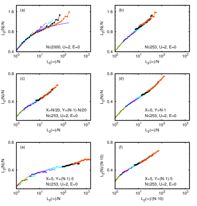
Figure 18: Comparison of scaling curves shown in the zoomed region $1\leq L_{2}(\infty)/N\leq 1500$ for $U=2$ and $E=0$ for different cases concerning the range of used system sizes and the determination of $L_{2}(N)$ from the two-particle Green function. Panel (a) shows the same scaling curve as in the left panel of Figure 11, i. e. $L_{2}(N)$ is given by (22) and $L_{2}(\infty)$ has been determined from data points with $50\leq N\leq 2000$ and $N\geq 1.5\,L_{1}$. However, in panel (a) also the non-used data points with $50\leq N<1.5\,L_{1}$ are shown. The blue full curve in panel (a) corresponds to the same fit of the scaling curve shown in the left panel of Figure 11. In panels (b)-(f) a (denser) set of data points for smaller system sizes $50\leq N\leq 253$ is used. In panel (b) $L_{2}(N)$ is given by (22) as in panel (a) while in panels (c)-(f) $L_{2}(N)=L_{G}(X,Y,N,0)$ as defined in (21) with $X=N/20$ and $Y=(N-1)-N/20$ [panel (c)], $X=0$ and $Y=N-1$ [panel (d)], $X=5$ and $Y=(N-1)-5$ using $N$ as system size for the scaling [panel (e)] and $X=5$ and $Y=(N-1)-5$ using the reduced effective system size $N-10$ for the scaling [panel (f)]. The used disorder values and corresponding colors are as in Figure 11 but due to the zoomed range only the data points for the 7-8 smallest disorder values are visible.

To investigate in more detail the issues of limited system size and also of the precise choice for the definition of the two-particle localization length in terms of the projected Green function, we computed (with 1% accuracy) special data sets of smaller system sizes $50\leq N\leq 253$, with an approximate ratio $1.1$ between two neighbor values of $N$. To be more precise we determined for these limited system sizes our variant (22) of the two-particle localization length $L_{2}(N)$ and of some other variants with different parameters in (21), including the two cases of song1 ; leadbeater1 . The results of this comparative study of “scaling in the invalid regime” (with $N\leq 253<L_{1}=420$ for $W=0.5$) are shown in Figure 18 for the case $U=2$ and $E=0$.

First we present again in panel (a) of Figure 18 the same “correct” scaling curve of the left panel of Figure 11 in a zoomed presentation and computed with data for $L_{2}(N)$, given by (22), with $50\leq N\leq 2000$ and $N\geq 1.5L_{1}$. However in addition also the non-used data points with $N<1.5L_{1}$ are shown for illustration but these data points were not used for the computation of the scaling curve. We indeed observe that they are clearly outside (above) the scaling curve thus confirming the condition $N>L_{1}$ for the validity of the one-parameter scaling approach.

In panel (b) the scaling curve of the same quantity (22) but using the data set for smaller system sizes $N\leq 253$ is visible. The quality of the scaling curve appears to be rather satisfactory but its form is very different from the scaling curve of panel (a) or Figure 11. In particular it does not have a finite limit for large $L_{2}(\infty)/N$ which is indeed quite unusual if compared to the standard form of the scaling curves for the non-interacting Anderson model in 2 dimensions. The curve (b) can be obtained from (a) by removing in the latter the “good” data points (with $N>253$) in the lower parts of the individual curves and then using the “bad” data points (those with $N<L_{1}$) to recalculate the scaling parameters. This changes considerably the form of the scaling curve and reduces the values of infinite size localizations lengths for small disorder values.

Panel (c) shows, also for the case $N\leq 253$, the scaling curve of a different quantity $L_{2}(N)=L_{G}(N/20,N-1-N/20,N,0)$ corresponding to two reference positions 5% inside the sample and absence of the denominator $|\bar{G}(x,x)|$ in (21). The scaling curve of panel (d) is similar but for the quantity $L_{2}(N)=L_{G}(0,N-1,N,0)$ with two reference positions exactly at the boundary (and also absence of the denominator $|\bar{G}(x,x)|$) which corresponds exactly to the choice of song1 . We note that the scaling curves of (b), (c), and (d) have a rather similar form and slightly increasing values for large $L_{2}(\infty)/N$.

In panel (e) we consider the case of $L_{2}(N)=L_{G}(p,N-1-p,N,0)$ for $p=5$ corresponding to reference positions 5 sites inside the sample which is similar (or even identical) to the choice of leadbeater1 . The scaling curve has a very different form than the three previous cases. The matching of the different data points is not very good and one observes small but clearly significant and systematic deviations from a perfect scaling. More importantly the obtained infinite size localization lengths at smallest disorder are strongly increased as compared to all previous cases. The question arises why we observe this strong difference, especially between the two scenarios (e) and (c) where for both cases the two reference positions are slightly inside the sample ? The reason is that for (e) the distance between the two reference positions is effectively $N_{\rm eff}=N-10$ instead of $N$ and therefore the scaling procedure should be done with this effective system size which provides indeed a non-trivial complicated transformation as can be seen in panel (f) where the same data of (e) is submitted to a scaling procedure using $N_{\rm eff}=N-10$ as effective system size. The scaling curve of (f) is very different from (e) but quite similar in form to the cases (b), (c) and (d).

For the case (c) we have also a reduced effective system $N_{\rm eff}=0.9N$ but here the situation is very different since this transformation corresponds in double logarithmic scale to a simple small shift up and to the right of all data and the scaling curve. Actually this transformation maps somehow the case of (c) to the case of (d) (with reference points precisely at the boundaries). Therefore the resulting infinite size localization lengths are not modified when using a scaling procedure with $N_{\rm eff}=0.9N$ instead of $N$. However, the transformation $N_{\rm eff}=N-10$ affects seriously in a non-trivial way the form of the individual data curves (also in double logarithmic scale) and modifies strongly the obtained infinite size localization lengths. Therefore it is indeed necessary to be careful when using offset parameters by choosing reference positions slightly inside the sample. A constant choice of them independent of $N$ will produce tainted scaling results and one must instead choose them proportional to $N$, for example 5% inside the sample.

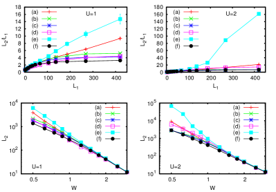
Figure 19: Comparison of $L_{2}$ obtained by the six different cases (a)-(f) of finite size scaling illustrated in Figure 18 for $E=0$ (all panels), and $U=1$ (left panels) or $U=2$ (right panels). Top panels show the enhancement factor $L_{2}/L_{1}$ versus $L_{1}=105/W^{2}$ and bottom panels show $L_{2}$ versus $W$ on a double logarithmic scale. Top panels also show error bars obtained by the scaling procedure and the absence or non-visibility of them indicates errors below point size except in top right panel for the two data points of curve (e) with largest values of $L_{1}$ and $L_{2}/L_{1}$ which have infinite errors. In the bottom panels errors are always below point size except in bottom right panel for the two points of curve (e) with largest values of $L_{1}$ and $L_{2}$ corresponding to infinite errors.

Figure 19 shows the dependence of the infinite size localization lengths on $L_{1}$ or $W$ (for $E=0$ and two interaction values $U=1$ and $U=2$) obtained by the different scaling scenarios (a)-(f) of Figure 18. The cases (b), (c), (d) and (f), all obtained for small system sizes $N\leq 253$, seem to form one group with roughly comparable results and only slight deviations among them indicating that the precise choices of $L_{2}(N)$ either by (22) or (21) with different parameters is not very important in this context. However, they all produce significantly smaller values of infinite size localization lengths for large $L_{1}$ (small $W$) than the scenario (a) which is the only case with large system sizes up to $N=2000$ ensuring that the important condition $N\geq 1.5L_{1}$ is verified for a sufficient number of data points. The scenario (e), also valid for small system sizes, suffers additionally from the constant offset of the reference points in the definition of $L_{2}(N)$ which seriously taints the scaling results and produce for large $L_{1}$ considerably larger values of infinite size localization lengths than the case (a). Actually, for $U=2$ there is only one (usable) data point in the second last curve having an overlap with the third last curve and resulting formally in an infinite margin of error for the two last localization lengths which are by a factor $\sim 10$ larger than for $U=1$.

We mention that using the procedure (d) for $U=1$, $E=0$, $W=0.5$ we find the value $L_{2}=1863\pm 62$ which coincides very well with the value $L_{2}\approx 1900$ of song1 . Furthermore, using the procedure (e) for the same parameters we obtain $L_{2}=6179\pm 576$ which also agrees with the value $L_{2}\approx 6500$ of leadbeater1 (within margin of error). These agreements confirm that the raw data for the projected Green function of song1 ; leadbeater1 are in agreement with our raw data (obtained by a different and more efficient but equivalent method to compute the projected Green function). Of course both of these values are incorrect since there were obtained by scaling procedures which suffer from one or two serious flaws as explained above and the correct value is $L_{1}=3922\pm 102$ obtained by the procedure (a) using large system sizes up to $N=2000$ and the expression (22) for the definition of $L_{2}(N)$. In all figures and discussions of Section 5 and of Appendix B the quantity $L_{2}$ represents always the infinite size value obtained by finite size scaling from $L_{2}(N)$ for the case (a).

We mention that also for the two IPR length scales $\xi_{x}$ and $\xi_{\rm CM}$ considered in Section 4 the data with $N<2L_{1}$ do not obey one-parameter scaling. In this case these data produce for small disorder a maximum in the individual curves and quite strongly decaying values right to this maximum. This behavior is somewhat different as compared to the increasing curves visible in panel (a) of Figure 18 but it provides further confirmation that the application of one-parameter scaling theory to TIP indeed requires $N$ being sufficiently larger than $L_{1}$.

References

- (1) Patrick A. Lee and T. V. Ramakrishnan, Rev. Mod. Phys. 57, 287 (1985).
- (2) A. MacKinnon, and B. Kramer, Phys. Rev. Lett. 47, 1546 (1981).
- (3) A. MacKinnon, and B. Kramer, Z. Phys. B 53, 1 (1983).
- (4) B. Kramer and A. MacKinnon, Rep. Prog. Phys. 56, 1469 (1993).
- (5) K. B. Efetov, Supersymmetry in Disorder and Chaos, Cambridge University Press (1997).
- (6) T. Guhr, A. Müller-Groeling, and H. A. Weidenmüller, Phys. Rep. 299, 189 (1998).
- (7) C. W. J. Beenakker, Rev. Mod. Phys. 69, 731 (1997).
- (8) P. W. Brouwer and K. Frahm, Phys. Rev. B 53, 1490 (1996).
- (9) O. N. Dorokhov, Zh. Eksp. Teor. Fiz. 98, 646 (1990) [Sov. Phys. JETP 71, 360 (1990)].
- (10) D. L. Shepelyansky, Phys. Rev. Lett. 73, 2607 (1994).
- (11) M. Screiber, S.S. Hodgman, P. Bordia, H. Lüschen, M.H. Fischer, R. Vosk, E. Altman, U. Schneider, and I. Bloch, Science 349, 842 (2015).
- (12) Y.Imry, Europhys. Lett. 30, 405 (1995).
- (13) D. C. Thouless, Phys. Rev. Lett. 39, 1167 (1977).
- (14) K. Frahm, A. Müller–Groeling, J.-L. Pichard, and D. Weinmann, Europhys. Lett. 31, 169 (1995).
- (15) D. Weinmann, A. Müller–Groeling, J.-L. Pichard, and K. Frahm, Phys. Rev. Lett. 75, 1598 (1995).
- (16) P. Jacquod and D. L. Shepelyansky, Phys. Rev. Lett. 75, 3501 (1995).
- (17) Y. V. Fyodorov and A. D. Mirlin, Phys. Rev. B 52, R11580 (1995).
- (18) K. Frahm and A. Müller–Groeling, Europhys. Lett. 32, 385 (1995).
- (19) F. Borgonovi and D. L. Shepelyansky, Nonlinearity 8, 877 (1995).
- (20) F. Borgonovi and D. L. Shepelyansky, J. Phys. I France 6, 287 (1996).
- (21) O. Halfpap, A. MacKinnon and B. Kramer, Solid State Communications 107, 379 (1998).
- (22) F. von Oppen, T. Wetting, and J. Müller, Phys. Rev. Lett. 76, 491 (1996).
- (23) Ph. Jacquod, D. L. Shepelyansky, and O. P. Sushkov, Phys. Rev. Lett. 78, 923 (1997).
- (24) D. L. Shepelyansky, Proceedings of les Rencontres de Moriond 1996 on “Correlated Fermions and Transport in Mesoscopic Systems”, edited by T. Martin, G. Montambaux and J. Trân Thanh Vân, 201 (1996).
- (25) I. V. Ponomarev and P. G. Silvestrov, Phys. Rev. B 56, 3742 (1997).
- (26) R. A. Roemer, M. Schreiber and T. Vojta, phys. stat. sol. (b) 211, 681 (1999).
- (27) K. Frahm, A. Müller–Groeling, and J.- L. Pichard, Phys. Rev. Lett. 76, 1509 (1996).
- (28) K. Frahm, A. Müller–Groeling, and J.- L. Pichard, Z. Phys. B 102, 261 (1997).
- (29) J. Richert and H. A. Weidenmüller, J. Phys. A: Math. Gen. 36, 3281 (2003).
- (30) J. Richert and H. A. Weidenmüller, Annals of Physics 306, 96 (2003).
- (31) D. Weinmann, J.-L. Pichard, Phys. Rev. Lett. 77, 1556 (1996).
- (32) E. Akkermans and J.-L. Pichard, Eur. Phys. J. B 1, 223 (1998).
- (33) X. Waintal, and J.-L. Pichard, Eur. Phys. J. B 6, 117 (1998).
- (34) X. Waintal, D. Weinmann, and J.-L. Pichard, Eur. Phys. J. B 7, 451 (1999).
- (35) S. De Toro Arias, X. Waintal, and J.-L. Pichard, Eur. Phys. J. B 10, 149 (1999).
- (36) R.A. Römer and M. Schreiber, Phys. Rev. Lett. 78, 515 (1997).
- (37) R.A. Römer and M. Schreiber, Phys. Rev. Lett. 78, 4890 (1997).
- (38) K. M. Frahm, A. Müller-Groeling, J.-L. Pichard and D. Weinmann, Phys. Rev. Lett. 78, 4889 (1997).
- (39) P. H. Song and F. v. Oppen, Phys. Rev. B 59, 46 (1999).
- (40) P. H. Song and Doochul Kim, Phys. Rev. B 56, 12217 (1997).
- (41) M. Leadbeater, R. A. Römer, and M. Schreiber, Eur. Phys. J. B 8, 643 (1999).
- (42) K. M. Frahm, Eur. Phys. J. B, 10, 371 (1999).
- (43) D. O. Krimer, R. Khomeriki, S. Flach, JETP Letters 94, 406 (2011)
- (44) D. O. Krimer, S. Flach, Phys. Rev. B 91, 100201(R) (2015).
- (45) K. M. Frahm and D. L. Shepelyansky, Eur. Phys. J. B 88, 337 (2015).
- (46) S. Flach, M. Ivanchenko, and R. Khomeriki, Europhys. Lett. 98, 66002 (2012).
- (47) G. W. Stewart, Matrix Algorithms Volume II: Eigensystems, SIAM (2001).
- (48) K. M. Frahm, and D. L. Shepelyansky, Eur. Phys. J. B 76, 57 (2010).
- (49) H. R. Schwartz, Numerische Mathematik, B. G. Teubner, Stuttgart (1986).
- (50) K. M. Frahm, http://www.quantware.ups-tlse.fr/QWLIB/tipdisorder1d, Accessed February (2016).
- (51) M. Ortuno and E. Cuevas, Europhys. Lett., 46, 224 (1999).