Mean flow generation in rotating anelastic two-dimensional convection

Abstract

We investigate the processes that lead to the generation of mean flows in two-dimensional anelastic convection. The simple model consists of a plane layer that is rotating about an axis inclined to gravity. The results are two-fold: firstly we numerically investigate the onset of convection in three-dimensions, paying particular attention to the role of stratification and highlight a curious symmetry. Secondly, we investigate the mechanisms that drive both zonal and meridional flows in two dimensions. We find that in general non-trivial Reynolds stresses can lead to systematic flows and, using statistical measures, we quantify the role of stratification in modifying the coherence of these flows.

I Introduction

Geophysical and astrophysical flows are often turbulent and characterised by the presence of a wide-range of temporal and spatial scales. It is often the case that systematic large-scale flows that vary on long timescales co-exist with shorter lived turbulent eddies. Famous examples of such large-scale flows are the zonal jets so visible at the surface of the gas giants Porco et al. (2003); Vasavada and Showman (2005), the turbulent jet stream of the Earth Vallis (2006) and the strong zonal and meridional flows in the interior of the Sun which are interpreted as the observed differential rotation and meridional circulationsSchou et al. (1998).

A central question for fluid dynamicists is then to determine the role of the smaller-scale turbulent flows in modifying the systematic (or mean) flows. In some cases the turbulence will act purely as a dissipation or friction and act so as to damp any mean flows that occur. However in certain circumstances (usually when rotation is important) the turbulence may act as an anti-friction McIntyre (2003) and play a key role in driving and maintaining the mean flows. This mechanism is complicated by the tendency of the mean flows to act back on the turbulence and modify its form; a process that often determines the saturation amplitude of the mean flows. These are complicated interactions and although much progress has been made (as discussed briefly below) there is still much that is not understood.

Here we focus on a simple model where the turbulence is driven by a thermal gradient leading to convection. Owing to its importance in planetary and stellar interiors, this has been an extremely well studied problem, with many theoretical and numerical studies performed both in Cartesian (local) Hathaway and Somerville (1983, 1986, 1987); Julien and Knobloch (1998); Saito and Ishioka (2011) and spherical (both shell and full sphere) geometries Miesch et al. (2000); Elliott et al. (2000); Christensen (2001, 2002); Brun and Toomre (2002); Browning et al. (2004); Gastine and Wicht (2012); Gastine et al. (2013). We note that, in order to capture some effects of vortex stretching in a spherical body, Busse (1970) introduced an annulus model for its relative simplicity. This geometry has been used in attempts to model the zonal flow on Jupiter. For example, Jones et al. (2003) used a rotating annulus model in a two-dimensional (2d) study and incorporated the possibility of boundary friction which allowed for the more realistic multiple jet solutions to be found more easily. Rotvig and Jones (2006) examined this annulus model more extensively and identified a bursting mechanism that occurs in the convection in some cases.

We wish to focus on the role of stratification in altering the dynamics of the mean flow and so focus on a simple plane layer model in two dimensions allowing us to access some parameter regimes more easily than in other, more complicated geometries. The plane layer model, when the axis of rotation is allowed to vary from the direction of gravity, can be used to represent a local region at different latitudes of a spherical body. This paper builds on previous, largely Boussinesq, studies in a Cartesian domain which are summarised here - though this is by no means a complete review.

Much of the previous work using a local model makes the Boussinesq approximation so that density variations are neglected except in the buoyancy force Boussinesq (1903); Spiegel and Veronis (1960). For example, Julien and Knobloch (1998) studied nonlinear convection cells in a rapidly rotating fluid layer with a tilted rotation vector. They performed an asymptotic analysis and concluded the orientation of the convection rolls affects the efficiency of mean flow generation. Hathaway and Somerville (1983) performed three-dimensional (3d) simulations of convection in layers with tilted rotation vectors and no slip boundary conditions. They found that the horizontal component of the rotation vector gives a preference for cells aligned with the rotation axis which produces dynamical changes that drive a mean flow. There have also been a number of studies analysing the role of shear flow in a rotating plane layer. Hathaway and Somerville (1987) considered Boussinesq convection in a rotating system with an imposed shear flow. The imposed flow was constant in depth, but varying in latitude. They found in the non-rotating case that the convection extracts energy from the mean flow and reduces the shear, but in the rotating case the convection can feed energy into the mean flow and increase the shear. Hathaway and Somerville (1986) studied the interaction between convection, rotation and flows with vertical shear. They performed 3d simulations with no slip boundary conditions and found that in cases with vertical rotation the convection becomes more energetic by extracting energy from the mean flow. However, for cases with a tilted rotation vector the results depend on the direction of the shear. Saito and Ishioka (2011) revisited the problem of the interaction of convection with rotation in an imposed shear flow. They were able to examine a larger region of parameter space than Hathaway and Somerville (1987) and identified a feedback mechanism in which the convection interacts with the rotation in such a way that leads to an accelerated mean flow. This mechanism operates when the sign of the shear flow is opposite to the vertical component of the rotation axis and relies upon the sinusoidal form of shear flow they imposed. Currie (2014) studied the generation of mean flows by Reynolds stresses in Boussinesq convection both in the absence and in the presence of a thermal wind and showed whether convection acts to increase or decrease the thermal wind shear depends on the fluid Prandtl number and the angle of the rotation vector from the vertical.

In many astrophysical systems the fluid is strongly stratified (e.g., in stellar and some planetary interiors) and therefore density changes across the layer (that are neglected by the Boussinesq approximation) may play a significant role. Therefore, there exist studies where fully compressible convection has been simulated Brummell et al. (1996, 1998); Chan (2001) but the full equations are computationally intensive to solve owing to the necessity of accurately tracking sound waves. However, for systems where there are a large number of scale heights involved but that remain close to being adiabatic, the anelastic equations are an improvement on the Boussinesq equations Gough (1969); Lantz and Fan (1999); Braginsky and Roberts (1995). Furthermore, the anelastic equations allow for density stratification across the layer whilst still filtering out fast sound waves thus making studying a compressible layer more computationally accessible.

In this paper we use the anelastic approximation to investigate the effects of stratification on both linear and nonlinear convection, focussing on the role stratification plays in altering the dynamics of mean flows. In other words, we extend the work of Hathaway and Somerville (1983) to include the important effects of stratification.

By considering density variations across the fluid layer one cannot take both the dynamic viscosity $\mu$ and the kinematic viscosity $\nu$ of the fluid to be constant (since $\mu=\rho\nu$ where $\rho$ is the fluid density) therefore, a choice has to made. Similarly, one cannot take both the thermal conductivity $k$ and the thermal diffusivity $\kappa$ of the fluid to be constant and again, a choice has to be made. The results can depend on these choices (see, e.g., Glatzmaier and Gilman (1981)). In this paper we consider a formalism where $\nu$ and $k$ are constant. Anelastic formalisms also differ depending on whether entropy or temperature is diffused in the energy equationBraginsky and Roberts (1995). If one diffuses entropy then temperature can be eliminated as a variable from the formulation; for simplicity, this is often the approach taken in nonlinear studies and is the choice we make here. Further differences between anelastic formalisms arise from whether one takes the vertical axis to be parallel or antiparallel to gravity. Typically, in Boussinesq formulations the vertical axis increases upwards, whereas in compressible studies it is taken downwards. In order to ease the comparison with Boussinesq models, we take the vertical axis to increase upwards in line with Mizerski and Tobias (2011). The existing studies of anelastic convection, linear and nonlinear, each consider a different formalism (discussed below) and therefore care has to be taken when comparing across the different models.

The onset of compressible convection in a local Cartesian geometry, using the anelastic approximation, has been studied in a number of papers. The earliest of these studies includes the work of Kato and Unno (1960) who studied the onset of convection in an isothermal reference atmosphere. As an alternative, it is common to assume a polytropic reference atmosphere, as we do here. For example, Jones et al. (1990) considered a polytropic, constant conductivity model in a Cartesian geometry in which rotation, magnetic field and gravity were taken to be mutually perpendicular. This is different to the configuration in this paper as we consider rotation that is oblique to gravity. More recently, Mizerski and Tobias (2011) investigated the effect of compressibility and stratification on convection, using the anelastic approximation, in a rotating plane layer model where rotation and gravity were aligned; they compared a model with constant $k$ with one with constant $\kappa$ whilst keeping $\nu$ constant throughout and they chose to diffuse entropy. In this paper we essentially consider the constant conductivity case of Mizerski and Tobias (2011) but we allow the rotation vector to tilt from the vertical in order to model behaviour at mid-latitudes of a spherical body. To date, the only other study examining the linear stability of compressible convection in this tilted f-plane geometry is that of Calkins et al. (2014) who compared the onset of convection in compressible and anelastic ideal gases on a tilted f-plane. The majority of the results from that paper are concerned with comparing the anelastic equations with temperature diffusion with the fully compressible equations, and so those results are not directly comparable with ours. They do however, also consider an entropy diffusion model but in contrast to the work here, they take $\mu$ constant and have the vertical axis pointing downwards.

In contrast to the Boussinesq systems, there have been relatively few studies of mean flow generation by convection under the anelastic approximation in a local model. Rogers and Glatzmaier (2005) did model penetrative convection in a system where a convective region is bounded below by a stable region and Rogers et al. (2003) presented 2d simulations of turbulent convection using the anelastic approximation in a non-rotating system. However, most relevant to the work we undertake here is the study of Verhoeven and Stellmach (2014) who used 2d anelastic simulations of rapidly rotating convection in the equatorial plane (gravity and rotation perpendicular) to support a compressional Rhines-type mechanism predicting the width of jets driven in such a rapidly rotating system. In their study, as we do, Verhoeven and Stellmach (2014) take $\nu$ constant and consider an entropy diffusion model, however, in contrast to our work, Verhoeven and Stellmach (2014) take $\kappa$ constant.

Our study, using a local model, allows us to focus on the effect of stratification on mean flow generation without many of the complicating features of a spherical geometry, say. However our model still incorporates some important physical features that are expected to play a role in the determining the dynamics of many astrophysical objects, namely stratification on the f-plane.

This paper is organised as follows: in section II, the model and governing equations are presented. In section III, we aim to add to the existing literature discussed above by carrying out 3d linear stability analysis and present a new symmetry of which technical details are given in an appendix. In section IV, we analyse the role of stratification in mean flow generation at mid-latitudes using a 2d local model, focussing on the differences from Boussinesq models. This work complements previous Boussinesq and fully compressible studies in a Cartesian domain, as well as the global anelastic models considering mean flows.

II Model setup and equations

We consider a local plane layer of convecting fluid rotating about an axis that is oblique to gravity, which acts downwards. The rotation vector lies in the $y$-$z$ plane and is given by $\bm{\Omega}=(0,\Omega\cos\phi,\Omega\sin\phi)$, where $\phi$ is the angle of the tilt of the rotation vector from the horizontal, so that the layer can be thought of as being tangent to a sphere at a latitude $\phi$. In this case, the $z$-axis points upwards, the $x$-axis eastwards and the $y$-axis northwards.

We denote the fluid density, pressure, temperature, entropy and velocity by $\rho$, $p$, $T$, $s$ and $\mathbf{u}=(u,v,w)$ respectively. The anelastic equations are then found by decomposing the thermodynamic variables into a reference state (denoted by the subscript _ref) and a perturbation. The reference state depends on $z$ only and is assumed to be almost adiabatic. The departure from adiabaticity is measured by a small parameter, $\epsilon$ given by

$$\epsilon\equiv\frac{d}{H_{r}}\left(\frac{\partial\ln T_{\rm{ref}}}{\partial\ln p_{\rm{ref}}}-\frac{\partial\ln T_{\rm{ref}}}{\partial\ln p_{\rm{ref}}}\bigg{|}_{\text{ad}}\right)=-\frac{d}{T_{r}}\left[\left(\frac{dT_{\rm{ref}}}{dz}\right)_{r}+\frac{g}{c_{p}}\right]=-\frac{d}{c_{p}}\left(\frac{ds_{\rm{ref}}}{dz}\right)_{r},$$ (1)

where $d$ is the layer depth, $H_{r}=\frac{p_{\rm{ref}}}{g\rho_{\rm{ref}}}=-\frac{{\rm d}z}{{\rm d}\ln p_{\rm{ref}}}$ is the pressure scale height, $c_{p}$ is the specific heat at constant pressure, $g$ is the acceleration due to gravity, the subscript ${}_{\text{ad}}$ indicates the value for an adiabatic atmosphere and a subscript _r denotes a value taken at the bottom of the layer, $z=0$. $\epsilon$ will also be a measure of the relative magnitude of the perturbations and we assume

$$\frac{|p|}{p_{\rm{ref}}}\approx\frac{|\rho|}{\rho_{\rm{ref}}}\approx\frac{|T|}{T_{\rm{ref}}}\approx|s|\approx\epsilon\ll 1,$$ (2)

so that the perturbations are small compared to the reference state.

It is useful to write the equations in a dimensionless form, using $d$ as the length scale and the thermal diffusion time $\frac{d^{2}}{\kappa_{r}}$ as the time scale, where $\kappa$ is the thermal diffusivity. In this case, the leading order equations are given by

$$\left[\frac{\partial\mathbf{u}}{\partial t}+(\mathbf{u}\cdot\nabla)\mathbf{u}\right]=-\nabla\left(\frac{p}{\rho_{\rm{ref}}}\right)+RaPrs\mathbf{\hat{e}_{z}}-Ta^{\frac{1}{2}}Pr\bm{\Omega}\times\mathbf{u}+\frac{Pr}{\rho_{\rm{ref}}}\nabla\cdot{\bm{\varsigma}},$$ (3)

$$\nabla\cdot(\rho_{\rm{ref}}{\mathbf{u}})=0,$$ (4)

$$\rho_{\rm{ref}}T_{\rm{ref}}\left[\frac{\partial{s}}{\partial t}+(\mathbf{u}\cdot\nabla)(s_{\rm{ref}}+s)\right]=\nabla\cdot[T_{\rm{ref}}\nabla(s_{\rm{ref}}+s)]-\frac{\theta}{\rho_{\rm{ref}}Ra}\frac{\bm{\varsigma}^{2}}{2},$$ (5)

$$\frac{p}{p_{\rm{ref}}}=\frac{T}{T_{\rm{ref}}}+\frac{\rho}{\rho_{\rm{ref}}},$$ (6)

$$s=\frac{1}{\gamma}\frac{p}{p_{\rm{ref}}}-\frac{\rho}{\rho_{\rm{ref}}},$$ (7)

where $\varsigma_{ij}=\rho_{\rm{ref}}\left[\frac{\partial u_{i}}{\partial x_{j}}+\frac{\partial u_{j}}{\partial x_{i}}-\frac{2}{3}(\nabla\cdot\mathbf{u})\delta_{ij}\right]$ is the stress tensor with $\bm{\varsigma}^{2}\equiv\bm{\varsigma}:\bm{\varsigma}=\varsigma_{ij}\varsigma_{ij}$. $\theta$ is the dimensionless superadiabatic temperature gradient and $\gamma$ is the ratio of specific heats at constant pressure to constant volume. In this case the dimensionless parameters are the Rayleigh, Taylor and Prandtl numbers given by

$$Ra=\frac{gd^{3}}{\kappa_{r}\nu},\mbox{\quad}Ta=\frac{4\Omega^{2}d^{4}}{\nu^{2}}\mbox{\quad and \quad}Pr=\frac{\nu}{\kappa_{r}},$$ (8)

respectively. Again, note in our formalism that we assume the kinematic viscosity $\nu$ and the turbulent thermal conductivity $k=\rho_{\rm{ref}}c_{p}\kappa$ (where we now interpret $\kappa$ as the turbulent thermal diffusivity) to be constant. Furthermore, we use a model that takes the turbulent thermal conductivity to be much larger than the molecular conductivity and so equation (5) contains an entropy diffusion term but not a thermal diffusion term; Braginsky and Roberts (1995) discuss models including both terms. In addition, we have employed a technique introduced by Lantz (1992) and Braginsky and Roberts (1995) to reduce the number of thermodynamic variablesLantz and Fan (1999); Jones and Kuzanyan (2009).

In this paper, we consider a time-independent, polytropic reference state given by

$$T_{\rm{ref}} =1+\theta z,\quad\rho_{\rm{ref}}=(1+\theta z)^{m},\quad p_{\rm{ref}}=-\frac{RaPr}{\theta(m+1)}(1+\theta z)^{m+1},$$ (9)

$$s_{\rm{ref}} =\frac{m+1-\gamma m}{\gamma\epsilon}\ln(1+\theta z)+\text{const}\text{ \quad with \quad}\frac{m+1-\gamma m}{\gamma}=-\frac{\epsilon}{\theta}=\mathcal{O}(\epsilon),$$ (10)

where $m$ is the polytropic index and $-1<\theta\leq 0$. We note in this model there is no adjustment of the reference state by any mean that may be generated.

The equations (3)-(7) are similar to those given in case (1) of Mizerski and Tobias (2011); the key difference here however is the introduction of a tilted rotation vector, $\mathbf{\Omega}=(0,\cos\phi,\sin\phi)$. In this formalism, the anelastic equations (3)-(7) reduce to the Boussinesq equations in the limit $\theta\rightarrow 0$ and so $\theta$ can be thought of as a measure of the degree of compressibility. However, a more intuitive measure is given by

$$\chi=\frac{\rho_{\rm{ref}}|_{\text{z=0}}}{\rho_{\rm{ref}}|_{\text{z=1}}}=(1+\theta)^{-m}.$$ (11)

As $\chi$ is increased, the density contrast across the layer is also increased. Furthermore, it is common in the literature to use $N_{\rho}$, the number of density scale heights, as a measure of the stratification. Note, $\theta$, $\chi$ and $N_{\rho}$ are related by the following relations: $N_{\rho}=\ln\chi=\ln(1+\theta)^{-m}$.

With the reference state specified, we solve the anelastic equations subject to impenetrable, stress free and fixed entropy boundary conditions.

III Linear theory

Here we perform linear stability analysis of the 3d system in order to obtain information about the preferred modes of convection at onset. We linearise the anelastic equations (3)-(5) by perturbing about a trivial basic state and neglecting terms quadratic in the perturbation quantities. We then assume the perturbations are given by

$$(s,w,\zeta) ={\rm Re}\left\{\left[S(z),W(z),Z(z)\right]e^{\mathrm{i}(kx+ly)+\sigma t}\right\}.$$ (12)

Here $k$ and $l$ are the $x$ and $y$ wavenumbers respectively such that $a^{2}=k^{2}+l^{2}$ and σ= σ_R + i σ_I = σ_R + i ω is the complex growth rate. $S(z)$ is the amplitude function for $s$, $W(z)$ is the amplitude function for $w$ and $Z(z)$ is the amplitude function for the vertical vorticity $\zeta=\frac{\partial v}{\partial x}-\frac{\partial u}{\partial y}$. Taking the $z$-component of the curl and double-curl of the momentum equation to eliminate the pressure, along with the entropy equation, results in the following equations for the amplitude functions $W$, $Z$ and $S$:

$$\sigma Z= Ta^{\frac{1}{2}}Pr\left[\sin\phi\left(DW+\frac{m\theta}{1+\theta z}W\right)+\cos\phi\mathrm{i}lW\right]$$

$$+Pr(D^{2}-a^{2})Z+\frac{Prm\theta}{1+\theta z}DZ,$$ (13)

$$-\sigma[D^{2}W-a^{2}W+\frac{m\theta}{1+\theta z}DW-\frac{m\theta^{2}}{(1+\theta z)^{2}}W]=RaPra^{2}S$$

$$+ Ta^{\frac{1}{2}}Pr[\sin\phi DZ+\frac{m\theta}{1+\theta z}\cos\phi\mathrm{i}kW+\cos\phi\mathrm{i}lZ]-PrD^{4}W+2Pra^{2}D^{2}W$$

$$- Pra^{4}W+\frac{3Prm(2-m)\theta^{4}}{(1+\theta z)^{4}}W+\frac{2Prm\theta}{1+\theta z}a^{2}DW+\frac{2Prm^{2}\theta^{2}}{3(1+\theta z)^{2}}a^{2}W$$

$$- \frac{2Prm\theta}{1+\theta z}D^{3}W+\frac{Prm(4-m)\theta^{2}}{(1+\theta z)^{2}}D^{2}W-\frac{3Prm(2-m)\theta^{3}}{(1+\theta z)^{3}}DW,$$ (14)

$$\sigma S-\frac{W}{1+\theta z}=\frac{1}{(1+\theta z)^{m}}(D^{2}-a^{2})S+\frac{\theta}{(1+\theta z)^{m+1}}DS,$$ (15)

to be solved subject to the boundary conditions:

$$S=0,\text{\quad}W=0,\text{\quad}DZ=0\text{\quad and \quad}D^{2}W+\frac{m\theta DW}{(1+\theta z)}=0\quad\text{on $z=0,1$}.$$ (16)

Note, to simplify notation, we have used $D^{n}$ to mean $\frac{d^{n}}{dz^{n}}$. We solve this linear eigenvalue problem using the built-in bvp4c solver of Matlab.

Since we assume a reference state that is close to being adiabatic, we use $m=1.495$ in all calculations. Berkoff et al. (2010) demonstrated that the anelastic approximation gives a good approximation to fully compressible calculations even when the reference state is super-adiabatic, finding a $2\%$ error even when $\epsilon\sim 10$; but as mentioned above, we prefer to remain close to the adiabatic state, where $m=1.5$.

III.1 Effect of $\chi$ on the onset of convection

Figure 1 (a)-(c) show the critical Rayleigh number, wavenumber and frequency against $N_{\rho}$ for north-south (NS) convection rolls with $Pr=0.1$ and $\phi=\frac{\pi}{4}$. NS convection rolls are those whose axis is aligned in the $y$-direction ($l=0$) and similarly, east-west (EW) convection rolls are those whose axis is aligned in the $x$-direction ($k=0$). These are distinct when $\phi\neq\frac{\pi}{2}$, i.e., when rotation is oblique to gravity. For NS rolls, we observe that solutions with a positive frequency and those with a negative frequency are distinct unlike in the Boussinesq case Chandrasekhar (1961) - we will examine this symmetry breaking in more detail in the next section. For small $Ta$, the negative branch is preferred but this changes to the positive branch as $Ta$ is increased. For the cases shown, the positive solution always has the smaller critical wavenumber and critical frequency. In addition, the minimum $Ra_{\text{crit}}$ occurs for $N_{\rho}>0$, with both the minimum $Ra_{\text{crit}}$ and the $N_{\rho}$ at which it occurs, increasing with $Ta$. Another feature of figure 1 (a)-(c) is the difference between the positive and negative frequency solutions; this can be seen in the larger variation of $k_{\text{crit}}$ with increasing $N_{\rho}$ for the positive case. In a similar study, Calkins et al. (2014) found that the critical Rayleigh number is a monotonic function of stratification. This difference could arise because of a number of different modelling choices. First, as discussed in the introduction, Calkins et al. (2014) take constant $\mu$ where we have constant $\nu$. Second, the parameter regime considered is very different to that covered here; they choose to focus on the rapidly rotating case ($Ta\sim 10^{10}$) at $Pr=1$. Finally, and perhaps most importantly, the definition of $Ra$ is different between our models (the difference resulting from the fact that we take $z$ pointing upwards and $\nu$ constant in contrast to Calkins et al. (2014) who take $z$ pointing downwards and $\mu$ constant.) Indeed, Calkins et al. (2014) do comment that their critical Rayleigh number is not a monotonic function of stratification if evaluated away from the bottom boundary. We note that for vertical rotation we should recover the linear results of Mizerski and Tobias (2011) and indeed we do (though we do not present that case here). These differences highlight the important role of stratification in modifying the convection since the results are sensitive to whether $\mu$ or $\nu$ is held constant in the model as well as where $Ra$ is defined.

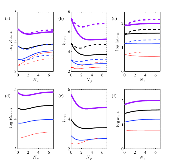
Figure 1: Critical Rayleigh number (a), (d), wavenumber (b), (e) and frequency (c), (f) against $N_{\rho}$ for NS (a)-(c) and EW (d)-(f) rolls when $Pr=0.1$, $\phi=\frac{\pi}{4}$. Solid lines represent solutions with $\omega_{\text{crit}}>0$ and dashed lines represent solutions with $\omega_{\text{crit}}<0$. In red (thinnest line) $Ta=10^{4}$, in blue (thin line) $Ta=10^{5}$, in black (thick line) $Ta=10^{6}$ and in purple (thickest line) $Ta=10^{7}$.

Figure 1 (d)-(f) show the equivalent to figure 1 (a)-(c) for EW rolls. Now, $k=0$, and there is no distinction to be made between the solutions with positive and negative frequency as they have the same critical values, hence we only plot the positive frequency solutions (we discuss this hidden symmetry in more detail in the next section). The behaviour is very similar to that in the NS case, but $Ra_{\text{crit}}$ is higher in the EW case, so that NS rolls are preferred, in agreement with Calkins et al. (2014) and also with linear Boussinesq systems, e.g., Hathaway et al. (1980).

III.2 Symmetry considerations

As highlighted in the previous section, when $\chi\neq 1$ ($N_{\rho}\neq 0$) and $l=0$ (NS rolls), there is a distinction to be made between solutions with a positive critical frequency and those with a negative critical frequency. However, when $k=0$ (EW rolls), even when $\chi\neq 1$, there is still a symmetry and the positive and negative branches have the same $|\omega_{\text{crit}}|$. We might expect that breaking the up-down symmetry of the system, via the introduction of a vertical density stratification, would cause a break in symmetry of the eigenvalue spectrum, and hence result in different frequencies for the positive and negative branches. Instead, when $k=0$, the eigenvalues remain in complex conjugate pairs. We see that in figure 2 (a) and (c), the introduction of a vertical stratification across the layer has, as expected, broken the symmetry of the eigenvalue spectrum - they no longer appear in complex conjugate pairs. However, counter-intuitively, when $k=0$ (subfigure(b)), the symmetry is not broken and the eigenvalues remain in complex conjugate pairs, in an analogous way to the Boussinesq case ($\chi=1$). Evonuk (2008) and Glatzmaier et al. (2009) describe a mechanism that is perhaps responsible for this difference between NS and EW rolls. The crux of their argument is that the vorticity equation (curl of equation (3)) contains a term proportional to $\bm{\Omega}(\nabla\cdot\mathbf{u})$, which is in general, non-zero for anelastic convection. However, in our system, the $x$-component of this term is zero and so it does not have an effect on EW rolls, whereas, the $y$-component of this term is non-zero and so it does have an effect on NS rolls.

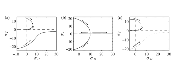
Figure 2: Real and imaginary parts of growth rate plotted against each other for different $Ra$ whilst $Ta=10^{5}$, $Pr=0.1$, $\phi=\frac{\pi}{4}$, $\chi\approx 31$. In (a) $l=0$, $k=3$, in (b) $k=0$, $l=3$ and in (c) $k=3$, $l=3$. The arrows indicate the direction of increasing $Ra$. When $k=0$ there exists an unexpected symmetry in the eigenvalue spectrum.

To investigate the symmetry of the EW solutions further, we look at the eigenfunctions, $|W(z)|$, $|Z(z)|$ and $|S(z)|$ as a function of depth as in figure 3. The eigenvalues, as explained before, are a complex conjugate pair for both $\chi$; in (a) $\sigma=8.0489\pm 11.3672\mathrm{i}$ and in (b) $\sigma=4.8626\pm 17.1070\mathrm{i}$. It is clear from the plots that, in the Boussinesq case, (a), the eigenfunctions are symmetric about $z=0.5$, whereas when a stratification is added, (b), the corresponding eigenfunctions possess no obvious symmetry, despite the fact the eigenvalues are a complex conjugate pair.

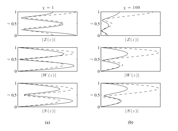
Figure 3: Eigenfunctions. The solutions $|W(z)|$, $|Z(z)|$ and $|S(z)|$ as a function of $z$ for $k=0$, $l=2$, $Ta=10^{5}$, $Pr=0.1$, $\phi=\frac{\pi}{4}$, $Ra=2\times 10^{5}$ and (a) $\chi=1$, (b) $\chi=100$. The solid line corresponds to the solutions with $\omega>0$ and the dotted lines to solutions with $\omega<0$.

This result is non-intuitive and so we give a proof of the maintenance of the symmetry when $k=0$. Essentially, the proof consists of forming the adjoint problem and then showing that the eigenvalue spectrum is symmetric; since the details are technical, they are included in the Appendix A.

IV Nonlinear results

This section extends the work of section III to the nonlinear regime, allowing us to examine the mean flows driven by the system. For these nonlinear results we restrict ourselves to the 2d system which lies in the plane of the rotation vector, the $y$-$z$ plane, i.e., $\frac{\partial}{\partial x}\equiv 0$.

We solve the nonlinear equations (3)-(7) using a streamfunction, $\psi(y,z)$, defined by

$$\rho_{\rm{ref}}\bm{u}=\rho_{\rm{ref}}u\bm{\hat{x}}+\nabla\times\psi(y,z)\bm{\hat{x}}=\left(\rho_{\rm{ref}}u,\frac{\partial\psi}{\partial z},-\frac{\partial\psi}{\partial y}\right).$$ (17)

and so $\nabla\cdot(\rho_{\rm{ref}}\mathbf{u})=0$ is automatically satisfied. We then write the equations in terms of $\psi$ and

$$\omega\equiv\nabla\times\mathbf{u}\cdot\hat{x}=-\frac{\nabla^{2}\psi}{\rho_{\rm{ref}}}-\frac{d}{dz}\left(\frac{1}{\rho_{\rm{ref}}}\right)\frac{\partial\psi}{\partial z},$$

and solve them for $\omega$, $u$, $s$ and $\psi$ using a Fourier-Chebyshev pseudospectral method with a second order, semi-implicit, Crank-Nicolson/Adams-Bashforth time-stepping scheme; for details see Currie (2014) and references within. $v$ and $w$ are then straightforward to obtain from $\psi$.

For diagnostic purposes, we decompose $\omega$, $u$, $s$ and $\psi$ into means (horizontal averages) and fluctuations; where the mean (denoted by an overbar) is defined as, for example,

$$\bar{u}(z,t)=\frac{1}{L}\int_{0}^{L}u(y,z,t)\,dy,$$ (18)

where $L$ is the length of the computational domain.

IV.1 Bifurcation structure and large-scale solutions

In the limit $\theta\rightarrow 0$ ($\chi\rightarrow 1$), our anelastic system reduces to a Boussinesq system. As is typically seen in the Boussinesq case, if $Ra$ is slowly increased from its critical value (with other parameters fixed) then the solutions in the anelastic system undergo a series of bifurcations. An example is shown in figure 4 which shows time series of the Nusselt number ($Nu$) at different $Ra$. We define $Nu$ to be the ratio of the total heat flux to the conductive heat flux in the basic state. Clearly the system undergoes a number of bifurcations via steady, oscillatory, quasiperiodic and chaotic solutions, en route to chaos (Ruelle-Takens-Newhouse route to chaos Ruelle and Takens (1971); Newhouse et al. (1978)). We note that some hysteresis of the solutions was observed, depending on the initial conditions used; however, a full investigation of the bistability is not examined here.

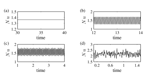
Figure 4: Time series of Nusselt number ($Nu$) for the case when $Pr=1$, $Ta=10^{5}$, $\phi=\frac{\pi}{4}$, $\chi=5$ and (a) $Ra=4\times 10^{4}$, (b) $Ra=4.2\times 10^{4}$, (c) $Ra=4.6\times 10^{4}$, (d) $Ra=7.5\times 10^{4}$.

Whilst it is typical for the system to undergo this series of bifurcations, Currie (2014) reported on a regime in which steady, large-scale solutions that are efficient at transporting heat by convection are found to exist in Boussinesq convection. Large-scale here means the largest scale possible in a box of a given size. In the Boussinesq system such solutions have also been seen in non-rotating 2d Rayleigh-Bénard convectionChini and Cox (2009); Hepworth (2014). In the anelastic system, we have found that such large-scale solutions are also able to exist even when the stratification is introduced; though interestingly, they may no longer correspond to steady (time-independent) solutions. For example, figure 5(a) shows a snapshot of the large-scale steady solution that exists when $\chi=1$, i.e., in the Boussinesq limit and 5(b) shows the equivalent large-scale solution when $\chi=10$. Whilst (a) corresponds to a steady solution, (b) is weakly time-dependent. For comparison, the dominant wavenumber of the equivalent solutions for the cases in figure 4, is about four times that of these large-scale solutions (e.g., see figure 5(c)). It is important to note that here we only consider $L=5$, but we would expect the width of the computational domain to have an effect on the emergence of the large-scale solutions. In general, a more detailed parameter study, which we do not carry out here, is required to examine more closely in which regimes such large-scale solutions exist.

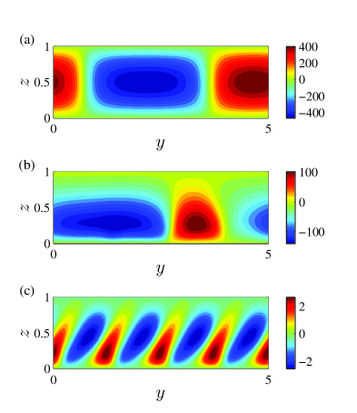
Figure 5: Contours of $\psi(y,z)$ for solutions when $L=5$, $Ra=8\times 10^{5}$, $Ta=10^{5}$, $Pr=1$, $\phi=\frac{\pi}{6}$, (a) $\chi=1$ and (b) $\chi=10$. (c) shows $\psi(y,z)$ for the parameters in figure 4 (a).

Though the existence of large-scale solutions is of interest, the primary aim of this paper is to determine the role of stratification in modifying mean flows.

IV.2 Generation of mean flows

We investigate how the strength and direction of mean flows driven in our plane layer system are affected by stratification. In all simulations presented we fix the length of our computational box to be $L=5$. To begin, we fix $Pr=1$, $Ra=2\times 10^{5}$, $Ta=10^{5}$, $\phi=\frac{\pi}{4}$ and consider $\bar{u}$ and $\bar{v}$ for three different stratifications (see figure 6). In (a), $\chi=1.5$ (close to Boussinesq) in (b), $\chi=5$ and in (c), $\chi=10$. Even though the critical Rayleigh number changes with $\chi$ and $Ra$ is fixed in these cases, the degree of supercriticality is not vastly changed - ranging from approximately 5.8 to 6.2 times the onset value. A striking feature present in all of the flows shown in figure 6 is that of strong oscillations. These oscillations are likely to be inertial oscillations that arise here because the Rossby number is of order one and so rotation and convection are of roughly equal importanceBatchelor (1967). Such oscillations were also observed in the fully compressible calculations of Brummell et al. (1998). In figure 6 (a), where $\chi$ is close to one, i.e., almost Boussinesq, we see that the flows are almost symmetric but, when the strength of stratification is increased, the extent of the asymmetry of the mean flows is also increased. For example, the positive flow of $\bar{v}$ in the upper half-plane only just penetrates down into the lower half-plane for $\chi$ close to one, but for stronger stratification it penetrates further into the layer. $\bar{u}$ is more time-dependent and harder to interpret than $\bar{v}$, but the asymmetry is still evident. The asymmetry results from the fact that, with stress free boundaries, the horizontal mass flux must be zero. From figure 6, other effects of increasing the stratification appear to be that the maximum velocity achieved by the flow decreases as $\chi$ increases, but the flows become more systematic. By systematic we mean a flow with a definite mean in the sense that the velocity fluctuations (including oscillations) produce a significant mean when averaged in both horizontal space and time.

Our results share some common features with those found in previous 3d studies. For example, we see strong systematic shear flows driven when the rotation vector is oblique to gravity as were seen in the Boussinesq calculations of Hathaway and Somerville (1983) and the fully compressible calculations of Brummell et al. (1998). Furthermore, the asymmetries introduced in the layer when stratification is added are also present in the flows of Brummell et al. (1998). We also find that $\bar{u}$ and $\bar{v}$ are comparable in size; a similar feature is also found in Hathaway and Somerville (1983) and Brummell et al. (1998). This is likely to be a result of the horizontal periodic boundary conditions artificially enhancing the meridional flow. We also note that there are some differences between the flows driven here and those in the previous work of Hathaway and Somerville (1983) and Brummell et al. (1998). The most obvious difference being that the sense of $\bar{u}$ is reversed (whilst the sense of $\bar{v}$ coincides). We also tend to find that the percentage of energy in the mean flows compared to the total energy is larger in our cases. We expect these differences result from the difference in parameter regimes considered and also the 2d nature of our system.

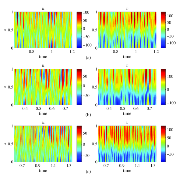
Figure 6: Contour plots of the mean flows $\bar{u}$ and $\bar{v}$. In (a) $\chi=1.5$, in (b) $\chi=5$ and in (c) $\chi=10$. In all cases $Pr=1$, $Ra=2\times 10^{5}$, $Ta=10^{5}$ and $\phi=\frac{\pi}{4}$.

To quantify the flow properties described above, we consider the mean and variation of the flows in time, and see how they vary with $\chi$ and $z$. In figure 7, we plot the time-averaged mean for $\bar{u}$ and $\bar{v}$ along with error bars corresponding to the standard deviation ($\Sigma$) from that mean. The first comment we make is that the error bars are significant and the departure of the maximum flow speed (given by the colorbars in figure 6) from the average is also significant; this is because of the oscillations present in the flows (as discussed above). Further, in (a) we see that $\Sigma(\bar{u})$ is smallest near to mid-layer and grows as we move out towards the boundaries but in (b), $\Sigma(\bar{u})$ is smallest at a deeper layer. This behaviour is also seen in $\Sigma(\bar{v})$, where for $\chi=1.5$, the standard deviation is fairly even across the layer but with its smallest value at approximately mid-layer; whereas for $\chi=10$, the smallest standard deviation is found at much smaller $z$. Note also, the mean of $\bar{u}$ and $\bar{v}$ is close to zero at $z=0.5$ in (a), but there is a significant flow at $z=0.5$ in (b). These measures characterise the behaviour we saw in the time-dependent plots in figure 6. As a percentage of its mean, $\Sigma(\bar{u})$ is larger than $\Sigma(\bar{v})$, indicative of the more time-dependent behaviour of $\bar{u}$ we also observed in figure 6 .

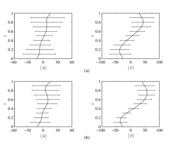
Figure 7: Mean (black curve) and standard deviation (error bars) of $\langle\bar{u}\rangle$ and $\langle\bar{v}\rangle$ for $Pr=1$, $Ra=2\times 10^{5}$, $Ta=10^{5}$, $\phi=\frac{\pi}{4}$ and (a) $\chi=1.5$, (b) $\chi=10$. As $\chi$ is increased the more systematic flow occurs at lower $z$.

Figure 8 shows how the standard deviation varies with $z$ for a number of different $\chi$. In general, we see that for stronger stratification $\Sigma$ is reduced. This behaviour is particularly evident in the lower depths of the layer (smaller z). It is also evident that for $\Sigma(\bar{v})$, the minimum of the standard deviation occurs at a deeper level in the layer as $\chi$ is increased. For $\Sigma(\bar{u})$, the trend is not so clear, however, the flows corresponding to larger $\chi$ have a minimum at a lower $z$ than the flows corresponding to smaller $\chi$. Therefore, there are fewer fluctuations at lower levels with increasing $\chi$, and it is this that results in the relatively large time-averaged mean at this level.

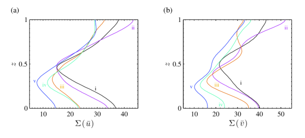
Figure 8: Standard deviation of (a) $\bar{u}$ and (b) $\bar{v}$ as a function of layer depth for different stratifications. In black (i) $\chi=1.5$, in purple (ii) $\chi=2$, in orange (iii) $\chi=5$, in turquoise (iv) $\chi=10$ and in blue (v) $\chi=100$.

Reynolds stresses are known to drive mean flows Hathaway and Somerville (1983); Brummell et al. (1998). To analyse their role in mean flow generation, we consider the mean equations obtained by horizontally averaging the $x$ and $y$ components of the momentum equation, i.e.,

$$Pr\rho_{\rm{ref}}\langle\bar{u}\rangle=\frac{Pr}{Ta^{\frac{1}{2}}\sin\phi}\frac{\partial}{\partial z}\left(\rho_{\rm{ref}}\frac{\partial\langle\bar{v}\rangle}{\partial z}\right)-\frac{1}{Ta^{\frac{1}{2}}\sin\phi}\frac{\partial(\rho_{\rm{ref}}\langle\overline{vw}\rangle)}{\partial z},$$ (19)

$$Pr\rho_{\rm{ref}}\langle\bar{v}\rangle=-\frac{Pr}{Ta^{\frac{1}{2}}\sin\phi}\frac{\partial}{\partial z}\left(\rho_{\rm{ref}}\frac{\partial\langle\bar{u}\rangle}{\partial z}\right)+\frac{1}{Ta^{\frac{1}{2}}\sin\phi}\frac{\partial(\rho_{\rm{ref}}\langle\overline{uw}\rangle)}{\partial z},$$ (20)

where we have averaged in time and assumed a statistically steady state so that $\frac{\partial}{\partial t}\langle\bar{u}\rangle=\frac{\partial}{\partial t}\langle\bar{v}\rangle=0$. The quantities $\rho_{\rm{ref}}\overline{uw}$, $\rho_{\rm{ref}}\overline{vw}$ are the Reynolds stresses terms, they measure the correlation between the horizontal and vertical velocity components. With a tilted rotation vector we might expect these correlations to be nonzeroHathaway and Somerville (1983). We note, from equations (19) and (20), that it is the $z$-derivative of $\rho_{\rm{ref}}\overline{vw}$ that drives $\bar{u}$ and the $z$-derivative of $\rho_{\rm{ref}}\overline{uw}$ that drives $\bar{v}$. In what follows, for both equations (19) and (20), we refer to the term on the LHS as the Coriolis term, the first term on the RHS as the viscous term and the second term on the RHS as the Reynolds stress (RS) term.

The factor of $\rho_{\rm{ref}}$ in the Coriolis terms of equations (19) and (20) means that, in theory, for two different $\chi$, if the driving terms on the right-hand side are of the same size, then the case with the largest $\chi$ will yield the largest $\bar{u}$ and $\bar{v}$, i.e., at any fixed $z$, if $Pr\rho_{\rm{ref}}\bar{u}$ is the same for two different $\rho_{\rm{ref}}$ (fixed $Pr$) then $\bar{u}$ will be larger for the smaller $\rho_{\rm{ref}}$. To see this, we plot each of the terms of equations (19) and (20) in figure 9; in addition, we plot $\bar{u}$ and $\bar{v}$ (without the $Pr\rho_{\rm{ref}}$ factors). For $\chi=1$, the Coriolis term is equivalent to the mean flow since $Pr=1$, therefore no additional line is visible in this case. However, for $\chi\neq 1$, there is a difference between the Coriolis term and the mean flow itself. In both (a) and (b), the strong dominance of the RS terms is clear. It is also evident that the viscous term is more important in determining $\bar{u}$ than it is $\bar{v}$, this is because the viscous term affecting each mean flow component depends on the gradient of the other mean flow component and we find that the gradient of $\bar{v}$ tends to be larger than that of $\bar{u}$. It is clear that the RS terms are larger in the $\chi=1$ case and this results in the Coriolis terms being larger for $\chi=1$. However, because for $\chi=10$, $\rho_{\rm{ref}}\leq 1$ across the layer, $\langle\bar{u}\rangle$ and $\langle\bar{v}\rangle$ are actually larger for $\chi=10$. This effect is most prominent at the top of the layer, where the fluid mass is at its lowest.

In the Boussinesq case, the RS terms are symmetric about the mid-layer depth. As a result of this symmetry, and because the RS terms are the dominant terms in equations (19) and (20), the mean flows are also symmetric about the mid-layer depth. Moreover, if $\chi$ is increased, then the RS terms become asymmetric, leading to asymmetric mean flows. We comment that the symmetry of the RS terms can change both as a result of the small-scale turbulent interactions but also through the mean flow acting back on the turbulence.

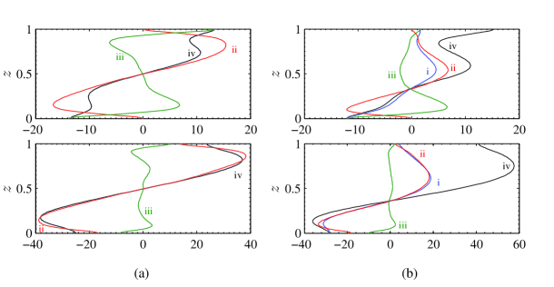
Figure 9: Terms of the mean flow equations (19) (top panels) and (20) (bottom panels) as a function of $z$ for $Pr=1$, $Ra=2\times 10^{5}$ and in (a), $\chi=1$, whilst in (b), $\chi=10$. The blue lines (i) represent the Coriolis terms, the red (ii) the RS terms, the green (iii) the viscous terms and black (iv) the mean flows $\langle\bar{u}\rangle$ and $\langle\bar{v}\rangle$. In case (a), the Coriolis terms are equivalent to the mean flows themselves.

V Conclusion

The results in this paper can be categorised into two distinct sections. The first section was concerned with linear anelastic convection. There we demonstrated and proved the existence of a previously unknown, hidden symmetry in the equations present when EW rolls are considered. We explained this by showing that the symmetry breaking term present in the vorticity evolution equation (introduced by the inclusion of a stratification) vanishes under certain circumstances.

The second part of the paper was concerned with the effect of stratification on nonlinear anelastic convection. We showed that efficient large-scale convection cells that have been shown to exist in 2d, Boussinesq Rayleigh-Bénard convection can also be found when stratification is introduced; although, unlike their Boussinesq counterparts, the anelastic solutions may not be time independent.

We went on to examine the effect of stratification on the generation of zonal and meridional mean flows. The use of an idealised 2d tilted plane layer model has allowed us to show the importance of correlations between velocity components resulting in Reynolds stresses that generate systematic flows. These flows have a strong time dependence but have a definite preferred direction on time averaging. The most striking difference between the flows driven in a stratified layer and their Boussinesq counterparts is seen in a vertical asymmetry. Although flow velocities tended to decrease with $\chi$, a statistical analysis showed that the mean flows become more systematic at lower layer depths the stronger the stratification. The asymmetry introduced by stratification is seen in the Reynolds stresses and we highlighted the role these stresses play in determining the size and vertical structure of the mean flows. In particular, even though the RS terms can be larger in the Boussinesq case, the flows are faster in the anelastic case because of the reduced fluid density in the layer. Whilst the Reynolds stresses dominated the flow size and structure, the viscous forces played a role in modifying the mean flows by opposing the Reynolds stresses (an effect that is to be expected at $Pr=1$). However, we would expect the viscous forces to be much less important in a realistic setting as the diffusivities are much smaller. In fact, Currie (2014) found small $Pr$ to play an important part in the dynamics of mean flow generation in Boussinesq convection. In particular, for the same size Reynolds stresses a larger mean flow is driven at smaller $Pr$. We would expect a similar effect to occur here as, from equations (19) and (20), the RS terms drive $Pr\rho_{\rm ref}\langle\bar{u}\rangle$ and $Pr\rho_{\rm ref}\langle\bar{v}\rangle$ and so for smaller $Pr$, $\rho_{\rm ref}\langle\bar{u}\rangle$ and $\rho_{\rm ref}\langle\bar{v}\rangle$ are indeed larger at any fixed height. The role of small $Pr$ in anelastic convection is currently under investigation.

There are some obvious shortcomings resulting from the simplicity of our model. For example, the periodic boundary conditions unrealistically enhance the meridional flow when in actuality, zonal flows are usually much larger than the meridional ones, in e.g., the Sun or on Jupiter. Despite this, our simple analysis has shown the importance of the Reynolds stresses in mean flow generation and shed some light on the role of stratification.

Owing to the existence of magnetic fields in physical systems such as stars and planets and their interaction with convection and rotation, an obvious question to ask is how such magnetic fields modify the mean flows generated. This is a question we address in a subsequent paper. We conclude by acknowledging the limitations of our simple model. Clearly in two dimensions correlations may be over-exaggerated leading to the formation of strong mean flows. We are therefore currently investigating how extending the model to three dimensions weakens correlations and affects the turbulent driving of mean flows.

*

Appendix A Proof

The following is a proof of the symmetry of the spectrum of eigenvalues that exists when $k=0$ (see section III.2). The proof not only holds for the stress free boundary conditions considered above but is a more general result and holds for all natural boundary conditions. The proof is similar in nature to that of Proctor et al. (2011) who prove a similar result. However, they consider a system with symmetric equations but break the symmetry through asymmetric boundary conditions. This is in contrast to this work, where we have asymmetric equations to begin with, and typically our boundary conditions are symmetric.

To begin the proof, we make a change of variables. Let

$$\tilde{Z} =(1+\theta z)^{\frac{m}{2}}Z,$$ (21)

$$\tilde{W} =(1+\theta z)^{\frac{m}{2}}W,$$ (22)

$$\tilde{S} =(1+\theta z)^{\frac{1}{2}}S,$$ (23)

then multiply (III) and (14) by $(1+\theta z)^{\frac{m}{2}}$, (15) by $({1+\theta z})^{m+\frac{1}{2}}RaPra^{2}$ and substitute in (21) - (23), to give

$$\sigma\tilde{Z}= Ta^{\frac{1}{2}}Pr\left[\sin\phi\left(D\tilde{W}+\frac{m\theta}{2(1+\theta z)}\tilde{W}\right)+\cos\phi\mathrm{i}l\tilde{W}\right]+$$

$$Pr(D^{2}-a^{2})\tilde{Z}-\frac{Prm\theta^{2}(\frac{m}{2}-1)}{2(1+\theta z)^{2}}\tilde{Z},$$ (24)

$$-\sigma[(D^{2}-a^{2})\tilde{W}-\frac{m\theta^{2}(1+\frac{m}{2})}{2(1+\theta z)^{2}}\tilde{W}]=RaPra^{2}(1+\theta z)^{\frac{m-1}{2}}\tilde{S}$$

$$+Ta^{\frac{1}{2}}Pr\sin\phi[D\tilde{Z}-\frac{m\theta}{2(1+\theta z)}\tilde{Z}]+Ta^{\frac{1}{2}}Pr\cos\phi\rm{i}l\tilde{Z}$$

$$-PrD^{4}\tilde{W}+2Pra^{2}D^{2}\tilde{W}-Pra^{4}\tilde{W}+\frac{Prm\theta^{2}(\frac{m}{2}+1)}{(1+\theta z)^{2}}D^{2}\tilde{W}$$

$$-\frac{Pr\theta^{3}m(m+2)}{(1+\theta z)^{3}}D\tilde{W}+\mathcal{F\tilde{W}}+Ta^{\frac{1}{2}}Pr\cos\phi\frac{m\theta}{1+\theta z}\mathrm{i}k\tilde{W},$$ (25)

where

$$\mathcal{F} =\frac{Prm\theta^{4}(3+\frac{5m}{4}-\frac{m^{2}}{4}-\frac{m^{3}}{16})}{(1+\theta z)^{4}}+\frac{Prma^{2}\theta^{2}(1+\frac{m}{6})}{(1+\theta z)^{2}},$$ (26)

and

$$\sigma RaPra^{2}(1+\theta z)^{m}\tilde{S}=RaPra^{2}(1+\theta z)^{\frac{m-1}{2}}\tilde{W}+RaPra^{2}(D^{2}-a^{2})\tilde{S}+\frac{RaPra^{2}\theta^{2}}{4(1+\theta z)^{2}}\tilde{S}.$$ (27)

When $k=0$, $a=l$ and we can write this system as

$$\sigma\mathbf{A}\mathbf{\tilde{X}}=\mathbf{B}\mathbf{\tilde{X}}$$ (28)

where $\mathbf{\tilde{X}}=\begin{bmatrix}\tilde{Z}\\ \tilde{W}\\ \tilde{S}\end{bmatrix},$ $\mathbf{A}=\begin{bmatrix}1&0&0\\ 0&-(D^{2}-l^{2})+\frac{m\theta^{2}(\frac{m}{2}+1)}{2(1+\theta z)^{2}}&0\\ 0&0&RaPrl^{2}(1+\theta z)^{m}\end{bmatrix}$ and $\mathbf{B}=$

$$\begin{bmatrix}\hbox{\multirowsetup$Pr(D^{2}-l^{2})-\frac{Prm\theta^{2}(\frac{m}{2}-1)}{2(1+\theta z)^{2}}$}&Ta^{\frac{1}{2}}Pr[\sin\phi(D+\frac{m\theta}{2(1+\theta z)})&\hbox{\multirowsetup$0$}\\ &+\cos\phi\mathrm{i}l]&\\ &&\\ Ta^{\frac{1}{2}}Pr[\sin\phi(D-\frac{m\theta}{2(1+\theta z)})&-Pr(D^{2}-l^{2})^{2}+\frac{Prm\theta^{2}(\frac{m}{2}+1)}{2(1+\theta z)^{2}}D^{2}&\hbox{\multirowsetup$RaPrl^{2}(1+\theta z)^{\frac{m-1}{2}}$}\\ +\cos\phi\mathrm{i}l]&-\frac{Pr\theta^{3}m(m+2)}{(1+\theta z)^{3}}D+\mathcal{F}&\\ &&\\ 0&RaPrl^{2}(1+\theta z)^{\frac{m-1}{2}}&RaPrl^{2}[(D^{2}-l^{2})+\frac{\theta^{2}}{4(1+\theta z)^{2}}]\end{bmatrix}.$$

Next, we define the inner product

$$\langle\mathbf{\tilde{X}_{1}},\mathbf{\tilde{X}_{2}}\rangle=\int_{0}^{1}\mathbf{\tilde{X}_{1}}^{{*}^{T}}\mathbf{\tilde{X}_{2}}\,dz=\int_{0}^{1}(\mathbf{\tilde{X}_{2}}^{{*}^{T}}\mathbf{\tilde{X}_{1}})^{*}\,dz=\langle\mathbf{\tilde{X}_{2}},\mathbf{\tilde{X}_{1}}\rangle^{*}$$ (29)

where

$$\mathbf{\tilde{X}_{1}}=\begin{bmatrix}\tilde{Z}_{1}\\ \tilde{W}_{1}\\ \tilde{S}_{1}\end{bmatrix},\hskip 14.22636pt\mathbf{\tilde{X}_{2}}=\begin{bmatrix}\tilde{Z}_{2}\\ \tilde{W}_{2}\\ \tilde{S}_{2}\end{bmatrix},$$ (30)

and $\mathbf{\tilde{X}_{1}}$ satisfies the same boundary conditions as $\mathbf{\tilde{X}_{2}}$. Then, since $\mathbf{A}$ is real and symmetric,

$$\langle\mathbf{\tilde{X}_{1}},(\sigma\mathbf{A}\mathbf{\tilde{X}_{2}}-\mathbf{B}\mathbf{\tilde{X}_{2}})\rangle =\int_{0}^{1}\mathbf{\tilde{X}_{1}}^{{*}^{T}}(\sigma\mathbf{A}\mathbf{\tilde{X}_{2}}-\mathbf{B}\mathbf{\tilde{X}_{2}})\,dz$$

$$=\int_{0}^{1}\mathbf{\tilde{X}_{2}}^{T}(\sigma^{*}\mathbf{A}\mathbf{\tilde{X}_{1}}-\mathbf{B}^{\dagger}\mathbf{\tilde{X}_{1}})^{*}\,dz=\langle(\sigma^{*}\mathbf{A}\mathbf{\tilde{X}_{1}}-\mathbf{B}^{\dagger}\mathbf{\tilde{X}_{1}}),\mathbf{\tilde{X}_{2}}\rangle.$$ (31)

Note, equation (A) only holds if the boundary conditions on $\mathbf{\tilde{X}_{i}}$ and $\mathbf{\tilde{X}_{i}}^{*}$ $(i=1,2)$ are the same. So $\mathbf{B}^{\dagger}$ is the formal adjoint of $\mathbf{B}$, i.e., $\langle\mathbf{u},\mathbf{B}\mathbf{v}\rangle=\langle\mathbf{B}^{\dagger}\mathbf{u},\mathbf{v}\rangle$ for vectors $\mathbf{u}$ and $\mathbf{v}$ and it is given by $\mathbf{B}^{\dagger}=$

$\begin{bmatrix}\hbox{\multirowsetup$Pr(D^{2}-l^{2})-\frac{Prm\theta^{2}(\frac{m}{2}-1)}{2(1+\theta z)^{2}}$}&-Ta^{\frac{1}{2}}Pr[\sin\phi(D+\frac{m\theta}{2(1+\theta z)})&\hbox{\multirowsetup$0$}\\ &+\cos\phi\mathrm{i}l]&\\ &&\\ -Ta^{\frac{1}{2}}Pr[\sin\phi(D-\frac{m\theta}{2(1+\theta z)})&-Pr(D^{2}-l^{2})^{2}+\frac{Prm\theta^{2}(\frac{m}{2}+1)}{2(1+\theta z)^{2}}D^{2}&\hbox{\multirowsetup$RaPrl^{2}(1+\theta z)^{\frac{m-1}{2}}$}\\ +\cos\phi\mathrm{i}l]&-\frac{Pr\theta^{3}m(m+2)}{(1+\theta z)^{3}}D+\mathcal{F}&\\ &&\\ 0&RaPrl^{2}(1+\theta z)^{\frac{m-1}{2}}&RaPrl^{2}[(D^{2}-l^{2})+\frac{\theta^{2}}{4(1+\theta z)^{2}}]\end{bmatrix}.$

Since $\mathbf{B}^{\dagger}$ is the formal adjoint of $\mathbf{B}$, its spectrum is the complex conjugate of the spectrum of B. Now, if we let

$$\mathbf{\tilde{Y}_{1}}=\begin{bmatrix}-\tilde{Z}_{1}\\ \tilde{W}_{1}\\ \tilde{S}_{1}\end{bmatrix},$$ (32)

then the adjoint equation

$$\sigma^{*}\mathbf{A}\mathbf{\tilde{X}_{1}} =\mathbf{B}^{\dagger}\mathbf{\tilde{X}_{1}}\quad\text{can be written as }$$ (33)

$$\sigma^{*}\mathbf{A}\mathbf{\tilde{Y}_{1}} =\mathbf{B}\mathbf{\tilde{Y}_{1}}\quad\text{ when }k=0.$$ (34)

So, if ($\sigma$, $\mathbf{\tilde{X}_{1}}$) is an eigenvalue, eigenfunction pair for the system then so is ($\sigma^{*}$, $\mathbf{\tilde{Y}_{1}}$).

Hence, we have shown that as long as the boundary conditions on $\mathbf{\tilde{X}}$ and $\mathbf{\tilde{X}}^{*}$ are the same, when $k=0$, the eigenvalue spectrum is symmetric. This is in agreement with the numerical results we found in section III.1.

If $k\neq 0$, then the final term on the right-hand-side of equation (A) is non-zero and must be added to the central entry of the matrices $\mathbf{B}$ and $\mathbf{B}^{\dagger}$; this results in a breakdown of the proof, as the last step (from equation (33) to equation (34)) can not be carried out. Therefore, when $k\neq 0$, the eigenvalue spectrum is not symmetric, again in agreement with the numerical results obtained in section III.1.

References

- Porco et al. [2003] C. C. Porco, R. A. West, A. McEwen, A. D. Del Genio, A. P. Ingersoll, P. Thomas, S. Squyres, L. Dones, C. D. Murray, T. V. Johnson, et al. Cassini imaging of jupiter’s atmosphere, satellites, and rings. Science, 299:1541, 2003.
- Vasavada and Showman [2005] A. R. Vasavada and A. P. Showman. Jovian atmospheric dynamics: An update after galileo and cassini. Rep. Prog. Phys., 68:1935, 2005.
- Vallis [2006] G. K. Vallis. Atmospheric and oceanic fluid dynamics: fundamentals and large-scale circulation. Cambridge University Press, 2006.
- Schou et al. [1998] J. Schou, H. M. Antia, S. Basu, R. S. Bogart, R. I. Bush, S. M. Chitre, J. Christensen-Dalsgaard, M. P. Di Mauro, W. A. Dziembowski, A. Eff-Darwich, et al. Helioseismic studies of differential rotation in the solar envelope by the solar oscillations investigation using the michelson doppler imager. Astrophys. J., 505:390, 1998.
- McIntyre [2003] M E. McIntyre. Solar tachocline dynamics: eddy viscosity, anti-friction, or something in between. Stellar Astrophysical Fluid Dynamics (ed. MJ Thompson & J. Christensen-Dalsgaard), page 111, 2003.
- Hathaway and Somerville [1983] D. H. Hathaway and R. C. J. Somerville. Three-dimensional simulations of convection in layers with tilted rotation vectors. J. Fluid Mech., 126:75, 1983.
- Hathaway and Somerville [1986] D. H. Hathaway and R. C. J. Somerville. Nonlinear interactions between convection, rotation and flows with vertical shear. J. Fluid Mech, 164:91, 1986.
- Hathaway and Somerville [1987] D. H. Hathaway and R. C. J. Somerville. Thermal convection in a rotating shear flow. Geophys. Astrophys. Fluid Dyn., 38:43, 1987.
- Julien and Knobloch [1998] K. Julien and E. Knobloch. Strongly nonlinear convection cells in a rapidly rotating fluid layer: the tilted f-plane. J. Fluid Mech., 360:141, 1998.
- Saito and Ishioka [2011] N. Saito and K. Ishioka. Interaction between thermal convection and mean flow in a rotating system with a tilted axis. Fluid Dyn. Res., 43:065503, 2011.
- Miesch et al. [2000] M. S. Miesch, J. R. Elliott, J. Toomre, T. L. Clune, G. A. Glatzmaier, and P. A. Gilman. Three-dimensional spherical simulations of solar convection. i. differential rotation and pattern evolution achieved with laminar and turbulent states. Astrophys. J., 532:593, 2000.
- Elliott et al. [2000] J. R. Elliott, M. S. Miesch, and J. Toomre. Turbulent solar convection and its coupling with rotation: The effect of prandtl number and thermal boundary conditions on the resulting differential rotation. Astrophys. J., 533:546, 2000.
- Christensen [2001] U. R. Christensen. Zonal flow driven by deep convection in the major planets. Geophys. Res. Lett., 28:2553, 2001.
- Christensen [2002] U. R. Christensen. Zonal flow driven by strongly supercritical convection in rotating spherical shells. J. Fluid Mech., 470:115, 2002.
- Brun and Toomre [2002] A. S. Brun and J. Toomre. Turbulent convection under the influence of rotation: sustaining a strong differential rotation. Astrophys. J., 570:865, 2002.
- Browning et al. [2004] M. K. Browning, A. S. Brun, and J. Toomre. Simulations of core convection in rotating a-type stars: differential rotation and overshooting. Astrophys. J., 601:512, 2004.
- Gastine and Wicht [2012] T. Gastine and J. Wicht. Effects of compressibility on driving zonal flow in gas giants. Icarus, 219:428–442, 2012.
- Gastine et al. [2013] T. Gastine, J. Wicht, and J. M. Aurnou. Zonal flow regimes in rotating anelastic spherical shells: An application to giant planets. Icarus, 225:156–172, 2013.
- Busse [1970] F. H. Busse. Thermal instabilities in rapidly rotating systems. J. Fluid Mech., 44:441, 1970.
- Jones et al. [2003] C. A. Jones, J. Rotvig, and A. Abdulrahman. Multiple jets and zonal flow on jupiter. Geophys. Res. Lett., 30, 2003.
- Rotvig and Jones [2006] J. Rotvig and C. A. Jones. Multiple jets and bursting in the rapidly rotating convecting two-dimensional annulus model with nearly plane-parallel boundaries. J. Fluid Mech., 567:117, 2006.
- Boussinesq [1903] J. Boussinesq. Théorie analytique de la chaleur: mise en harmonie avec la thermodynamique et avec la théorie mécanique de la lumière, volume 2. Gauthier-Villars, 1903.
- Spiegel and Veronis [1960] E. A. Spiegel and G. Veronis. On the boussinesq approximation for a compressible fluid. Astrophys. J., 131:442, 1960.
- Currie [2014] L. K. Currie. PhD thesis, University of Leeds, UK, 2014.
- Brummell et al. [1996] N. H. Brummell, N. E. Hurlburt, and J. Toomre. Turbulent compressible convection with rotation. i. flow structure and evolution. Astrophys. J., 473:494, 1996.
- Brummell et al. [1998] N. H. Brummell, N. E. Hurlburt, and J. Toomre. Turbulent compressible convection with rotation. ii. mean flows and differential rotation. Astrophys. J., 493:955, 1998.
- Chan [2001] K. L. Chan. Rotating convection in f-planes: Mean flow and reynolds stress. Astrophys. J., 548:1102, 2001.
- Gough [1969] D. O. Gough. The Anelastic Approximation for Thermal Convection. Journal of Atmospheric Sciences, 26:448, 1969.
- Lantz and Fan [1999] S. R. Lantz and Y. Fan. Anelastic Magnetohydrodynamic Equations for Modeling Solar and Stellar Convection Zones. Astrophys. J., 121:247, 1999.
- Braginsky and Roberts [1995] S. I. Braginsky and P. H. Roberts. Equations governing convection in earth’s core and the geodynamo. Geophys. Astrophys. Fluid Dyn., 79:1, 1995.
- Glatzmaier and Gilman [1981] G. A. Glatzmaier and P. A. Gilman. Compressible convection in a rotating spherical shell. iv-effects of viscosity, conductivity, boundary conditions, and zone depth. Astrophys. J., Supp. Ser., 47:103, 1981.
- Mizerski and Tobias [2011] K. A. Mizerski and S. M. Tobias. The effect of stratification and compressibility on anelastic convection in a rotating plane layer. Geophys. Astrophys. Fluid Dyn., 105:566, 2011. doi: 10.1080/03091929.2010.521748.
- Kato and Unno [1960] S. Kato and W. Unno. Convective instability in polytropic atmospheres, ii. Publ. Astron. Soc. Jpn., 12:427, 1960.
- Jones et al. [1990] C. A. Jones, P. H. Roberts, and D. J. Galloway. Compressible convection in the presence of rotation and a magnetic field. Geophys. Astrophys. Fluid Dyn., 53:145, 1990.
- Calkins et al. [2014] M. A. Calkins, K. Julien, and P. Marti. Onset of rotating and non-rotating convection in compressible and anelastic ideal gases. Geophys. Astrophys. Fluid Dyn., page 1, 2014.
- Rogers and Glatzmaier [2005] T. M. Rogers and G. A. Glatzmaier. Penetrative convection within the anelastic approximation. Astrophys. J., 620(1):432, 2005.
- Rogers et al. [2003] T. M. Rogers, G. A. Glatzmaier, and S. E. Woosley. Simulations of two-dimensional turbulent convection in a density-stratified fluid. Physical Review E, 67(2):026315, 2003.
- Verhoeven and Stellmach [2014] J. Verhoeven and S. Stellmach. The compressional beta effect: a source of zonal winds in planets? Icarus, 237:143, 2014.
- Lantz [1992] S. R. Lantz. PhD thesis, Cornell University, Ithaca, USA, 1992.
- Jones and Kuzanyan [2009] C. A. Jones and K. M Kuzanyan. Compressible convection in the deep atmospheres of giant planets. Icarus, 204:227, 2009.
- Berkoff et al. [2010] N. A. Berkoff, E. Kersalé, and S. M. Tobias. Comparison of the anelastic approximation with fully compressible equations for linear magnetoconvection and magnetic buoyancy. Geophys. Astrophys. Fluid Dyn., 104:545, 2010.
- Chandrasekhar [1961] S. Chandrasekhar. Hydrodynamic and Hydromagnetic Stability. Dover, 1961.
- Hathaway et al. [1980] D. H. Hathaway, J. Toomre, and P. A. Gilman. Convective instability when the temperature gradient and rotation vector are oblique to gravity. II - Real fluids with effects of diffusion. Geophys. Astrophys. Fluid Dyn., 15:7, 1980.
- Evonuk [2008] M. Evonuk. The role of density stratification in generating zonal flow structures in a rotating fluid. Astrophys. J., 673:1154, 2008.
- Glatzmaier et al. [2009] A. Glatzmaier, G, M. Evonuk, and T. M Rogers. Differential rotation in giant planets maintained by density-stratified turbulent convection. Geophys. Astrophys. Fluid Dyn., 103:31, 2009.
- Ruelle and Takens [1971] D. Ruelle and F. Takens. On the nature of turbulence. Commun. math. phys, 20:167–192, 1971.
- Newhouse et al. [1978] S. Newhouse, D. Ruelle, and F. Takens. Occurrence of strange axiom a attractors near quasi periodic flows on , . Commun. Math. Phys., 64:35, 1978.
- Chini and Cox [2009] G. P. Chini and S. M. Cox. Large Rayleigh number thermal convection: Heat flux predictions and strongly nonlinear solutions. Phys. Fluids, 21:083603, 2009.
- Hepworth [2014] B. J. Hepworth. PhD thesis, University of Leeds, UK, 2014.
- Batchelor [1967] G. K. Batchelor. An introduction to fluid dynamics. Cambridge university press, 1967.
- Proctor et al. [2011] M. R. E. Proctor, N. O. Weiss, S. D. Thompson, and N. T. Roxburgh. Effects of boundary conditions on the onset of convection with tilted magnetic field and rotation vectors. Geophys. Astrophys. Fluid Dyn., 105:82, 2011.