Explicit Conditions on Existence and Uniqueness of Load-Flow Solutions in Distribution Networks

Abstract

We present explicit sufficient conditions that guarantee the existence and uniqueness of the feasible load-flow solution for distribution networks with a generic topology (radial or meshed) modeled with positive sequence equivalents. In the problem, we also account for the presence of shunt elements. The conditions have low computational complexity and thus can be efficiently verified in a real system. Once the conditions are satisfied, the unique load-flow solution can be reached by a given fixed point iteration method of approximately linear complexity. Therefore, the proposed approach is of particular interest for modern active distribution network (ADN) setup in the context of real-time control. The theory has been confirmed through numerical experiments.

Nomenclature

$v=(v_{1},v_{2},...,v_{N})^{T}$	$v_{k}$ is the positive-sequence
	complex voltage at bus $k$.
$i=(i_{1},i_{2},...,i_{N})^{T}$	$i_{k}$ is the positive-sequence
	complex nodal current of bus $k$.
$s=(s_{1},s_{2},...,s_{N})^{T}$	$s_{k}$ is the complex nodal
	power injected into bus $k$.
bus $0$	Slack bus, with $v_{0}$=1 p.u.
$i_{0},s_{0}$	Slack bus complex nodal
	current and power.
$Y$	Positive-sequence nodal
	admittance matrix.
$Y_{LL}$	Square submatrix of $Y$,
	omitting the slack bus.
$w_{i}$, $i=1,...,N$	Positive-sequence complex voltage
	at node $i$ when $s$ is a zero vector.
$W=\mathop{\mathrm{diag}}(w_{i})$
$u=W^{-1}v$	Normalized node voltages.
(For any $z$ in $\mathbb{C}$) $\overline{z}$	The complex conjugate of $z$.

I Introduction

The load-flow problem, which expresses the link between complex node voltages and complex nodal power injections, is one of the main tasks in power system theory and applications. In the context of distribution networks, it is especially interesting to consider the case where non-slack buses are $PQ$ buses. In this paper we consider a network with one single slack bus, at which the complex voltage is assumed fixed and known, while the rest are $PQ$ buses. Given a vector of nodal power injections into $PQ$ buses, the problem is then to compute the vector of complex node voltages in the network that is feasible (i.e., close to $1$ p.u. in magnitude). In the rest of the manuscript, we make reference to the load-flow problem formulated for the positive sequence.

Due to the non-linearity of the equations, the existence and uniqueness of the solution to the load-flow problem is not guaranteed in general [1], [2], [3]. There is extensive literature on the subject as detailed in Section II. But for grid control, in order to maintain the system in feasible electrical states, it is essential to provide conditions guaranteeing that the implemented power setpoint leads to the unique feasible solution of the load-flow problem. Specifically, in active distribution networks (and particularly, microgrids), these conditions are further expected to be both explicitly formulated and verifiable in real-time.

There are multiple scenarios that have such expectations. One typical case is related to the islanding maneuver, namely the disconnection from the main grid due to an intentional or non-intentional decision (e.g., [4]). In particular, with respect to the non-intentional islanding, there is a need to evaluate in real-time whether a given resource can serve as a slack for the islanded microgrid [5]. This evaluation is based on verifying whether the currently implemented setpoint leads to the unique feasible solution of the corresponding load-flow problem. Another practical example is related to the recently introduced framework for performing real-time control of active distribution networks using explicit power setpoints [6]. In this framework, the knowledge of the current system state (obtained via a corresponding state estimation procedure) is assumed. A typical task in this framework is then to decide whether a given collection of power setpoints is admissible in the sense that the application of these setpoints will result in a feasible voltage profile of the grid. Hence as we can see from these situations, the research in this paper is of practical significance.

In the paper, we give explicit conditions that guarantee the existence and uniqueness of the load-flow solution for (possibly meshed) distribution networks with shunt elements. The unique solution can be reached by an iterative load-flow method given in this paper. Our conditions depend on the current state of the grid as well as on the requested power setpoints. The proposed approach is computationally efficient, with approximately linear complexity. Hence it can be applied in a real-time control framework. We also provide conditions in the “classical” setup, where the knowledge of the current grid state is absent. In this case, we show that our results are stronger than those introduced so far in the literature. Note that it is possible to extend our results to more general three-phase distribution networks, but this is the subject of ongoing work.

The paper is structured as follows. In Section II, we review the related work. In Section III, we present the load-flow problem and its useful equivalent formulation as a fixed point problem. In Section IV, we give our main result, and prove it in Section V. In Section VI, we provide numerical evaluation of our method. Finally, we conclude in Section VII.

II Related Work

In the last few decades, the existence and uniqueness of the solution to the load-flow problem have been studied from various perspectives.

In [7], conditions for the existence and uniqueness of the solution to reactive power-voltage magnitude problem are given and analyzed. Based on [7], [8] extends the result to active power-voltage angle problem. Under certain assumptions, by decoupling the active and reactive power (i.e., considering a sub-problem of active power with voltage angle, and a sub-problem of reactive power with voltage magnitude), sufficient conditions for load-flow solvability are explored. For balanced radial distribution networks, the uniqueness of a feasible load-flow solution is proved by exploiting the radial structure in [9]. In [10], the result is extended to the unbalanced radial three-phase distribution networks. However, all these results are based on certain assumptions and cannot be generically applied.

Recently, the focus has been moved to fixed point load-flow analysis since the fixed point theorem can guarantee the uniqueness of the load-flow solution. In fact, the first attempt of applying fixed point theorem to power systems dates back to [11], which focused on the study of convergence property of the Newton method. For the latest research, in [12], an efficient fixed point load-flow method is presented for radial distribution networks, but there is no further discussion about the convergence and solvability. Later, in [13], another form of fixed point load-flow method is proposed for distribution network with single slack bus. In the same paper, sufficient conditions are given to guarantee the existence and uniqueness of solution. These sufficient conditions are improved in [14].

In this paper, we use a fixed point formulation of the load-flow problem; then we specify a domain around a feasible point and provide sufficient conditions that guarantee the existence and uniqueness of load-flow solution in this domain. Under the proposed conditions, the unique solution can be reached using the fixed point iteration. It should be noticed that, by this approach, the feasibility of load-flow solution is usually preserved.

The theory proposed here shares some similarities with the fixed point load-flow methods established in [12], [13] and [14]. But, the method in [12] is a special case of this paper. Furthermore, the sufficient conditions in this paper are more general than the conditions in [13] and [14], and thus improve these results.

III The Load Flow Problem

We consider a distribution network modeled by its positive sequence equivalents with $N$ $PQ$ buses and one slack bus (in essence, a $V\theta$ bus). Without loss of generality, we assume that the complex voltage of the slack bus is $1$ p.u. Let $v=(v_{1},v_{2},...,v_{N})^{T}$ denote the vector of complex node voltages of the $PQ$ buses, $i=(i_{1},i_{2},...,i_{N})^{T}$ denote the vector of complex nodal currents into the $PQ$ buses, $i_{0}$ denote the complex nodal current into the slack bus, $s=(s_{1},s_{2},...,s_{N})^{T}$ denote the vector of complex nodal powers injected into the $PQ$ buses (negative value in real or imaginary part means consumed), and $s_{0}$ denote the complex nodal power injected into the slack bus. Also, for any complex number $z$, we denote its complex conjugate by $\overline{z}$. A similar notation holds for vectors and matrices.

As known, the nodal powers and nodal currents can be expressed in matrix form as

$$\left[\begin{array}[]{c}\overline{s}_{0}\\ \overline{s}\end{array}\right]=\left[\begin{array}[]{cc}1&\\ &\mathop{\mathrm{diag}}(\overline{v})\end{array}\right]\left[\begin{array}[]{c}i_{0}\\ i\end{array}\right],$$ (1)

$$\left[\begin{array}[]{c}i_{0}\\ i\end{array}\right]=Y\left[\begin{array}[]{c}1\\ v\end{array}\right].$$ (2)

Here, $Y$ is the $(N+1)\times(N+1)$ nodal admittance matrix of the system.

The classical load-flow problem in this setup is defined as follows: Given the nodal powers $s$, solve the set of equations (1) and (2) to obtain the nodal voltages $v$ and the power at the slack bus $s_{0}$. The nodal voltages are generally required to be feasible in the sense that all the node voltages have magnitude close to 1 p.u.

In this paper, we rely on an equivalent formulation of this problem that is known as implicit $Z_{bus}$ formulation, see e.g., [15]. First, partition the admittance matrix $Y$ as

$$Y=\left[\begin{array}[]{cc}Y_{00}&Y_{0L}\\ Y_{L0}&Y_{LL}\end{array}\right],$$ (3)

where $Y_{00}$ is a number, $Y_{0L}$ is a $1\times N$ row vector, $Y_{L0}$ is an $N\times 1$ column vector, $Y_{LL}$ is an $N\times N$ matrix. Now, we claim that $Y_{LL}$ is an invertible matrix. This fact was mentioned, e.g., in [13], without a proof; in Appendix A we give a proof that covers a broad range of distribution networks. The implicit $Z_{bus}$ formulation is then given by the following proposition; for completeness, we also provide a short proof.

Proposition 1.

The solution $v$ to the original load-flow problem can be found by solving the following fixed point equation

$$v=w+Y_{LL}^{-1}\mathop{\mathrm{diag}}(\overline{v})^{-1}\overline{s}\triangleq G(v),$$ (4)

$$\text{where}\qquad\qquad w\triangleq-Y_{LL}^{-1}Y_{L0}\hskip 85.35826pt$$ (5)

is given and is equal to the vector of complex voltages when power injections are zero (zero-load voltage of the grid).

Proof.

By (2) and (3), we have that

$$i=Y_{L0}+Y_{LL}v.$$

Thus, clearly, $w\triangleq-Y_{LL}^{-1}Y_{L0}$ is the zero-load voltage of the grid. From (1),

$$i=\mathop{\mathrm{diag}}(\overline{v})^{-1}\overline{s}$$

$$\text{and hence}\qquad\quad Y_{LL}^{-1}\mathop{\mathrm{diag}}(\overline{v})^{-1}\overline{s}=-w+v,\hskip 170.71652pt$$

which completes the proof. ∎

Remark 1.

This formulation can be viewed as a direct result of the superposition theorem: $v$ is the superposition of the voltages $w$, resulting from current injections by the slack bus when all other injections are absent ($s_{i}=0$, $i=1...N$) plus the voltages resulting from current injections due to $s$ when the slack bus injection is absent.

In the subsequent sections, we propose and prove sufficient conditions under which there exists a unique feasible solution to (4), which can be found by the iteration

$$v^{(k+1)}=w+Y_{LL}^{-1}\mathop{\mathrm{diag}}(\overline{v}^{(k)})^{-1}\overline{s}.$$ (6)

IV Main Result

In this section, we give conditions on the complex power injections $s$ which guarantee that iteration (6) converges to the unique feasible solution $v$ of the load-flow problem. We also provide computational complexity of the method.

Before presenting our method formally, we give a high-level outline. First, we assume the knowledge of a pair $(\hat{v},\hat{s})$ that satisfies the load-flow equations (4). This pair can be interpreted as the current (actual) state of the grid obtained via a measurement and state estimation process. In addition, we are given a desired “next” power setpoint $s$. Our conditions are thus formulated in terms of $(\hat{v},\hat{s})$ and $s$, and guarantee the unique feasible solution $v$ to (4) which is “close” to $\hat{v}$. Finally, we provide conditions on the starting point $v^{(0)}$ from which this solution can be computed using iteration (6).

As mentioned in the introduction, such a procedure is especially useful in the modern ADN setup, where the electrical state is continuously estimated and is varying slowly from its current value. In case there is no knowledge of the current state, a trivial choice for $(\hat{v},\hat{s})$ is $(w,\textbf{0})$, where $w$ is the zero-load voltage profile (5). For details, see Corollary 1 below.

IV-A Main Theorem

We introduce some further notation. Let $W\triangleq\mathop{\mathrm{diag}}(w)$ and set

$$\xi(s)\triangleq\|W^{-1}Y_{LL}^{-1}\overline{W}^{-1}\mathop{\mathrm{diag}}(\overline{s})\|_{\infty},$$ (7)

where, for any complex matrix $A$,

$$\|A\|_{\infty}\triangleq\max_{i}\sum_{j}|A_{ij}|$$

denotes the matrix norm induced by the $\ell_{\infty}$ norm. Let

$$u_{min}\triangleq\min_{j}\left|\hat{v}_{j}/w_{j}\right|.$$ (8)

Below is our main result. Its proof is in Section V.

Theorem 1.

Let the pair $(\hat{v},\hat{s})$ be a known solution to the load-flow problem (4). Consider some other candidate complex power injection $s$. Assume that

$$\xi(\hat{s})<u_{min}^{2}$$ (9)

$$\text{and}\qquad\Delta\triangleq\left(u_{min}-\frac{\xi(\hat{s})}{u_{min}}\right)^{2}-4\xi(s-\hat{s})>0.$$ (10)

Then there exists a unique solution $v$ to the load-flow problem, such that the pair $(v,s)$ satisfies (4) and $v$ belongs to

$$\mathcal{D}\triangleq\{v:\left|v_{i}-\hat{v}_{i}\right|\leq\rho\left|w_{i}\right|\}$$

$$\text{with}\qquad\qquad\rho\triangleq\frac{\left(u_{min}-\frac{\xi(\hat{s})}{u_{min}}\right)-\sqrt{\Delta}}{2}.\hskip 170.71652pt$$

Moreover, this solution can be reached using the iterative procedure (6) by starting with any $v^{(0)}\in\mathcal{D}$.

In case there is no knowledge of the current state $(\hat{v},\hat{s})$, the following corollary can be used.

Corollary 1.

Suppose that the complex power $s$ satisfies $\xi(s)<0.25$. Then, there exists a unique solution $v$ to the load-flow problem, such that the pair $(v,s)$ satisfies (4) and $v$ belongs to

$$\mathcal{D}^{\prime}\triangleq\left\{v:\left|v_{i}-w_{i}\right|\leq\frac{(1-\sqrt{1-4\xi(s)})\left|w_{i}\right|}{2}\right\}.$$

This solution can be reached using the iterative procedure in (6) by starting with any $v^{(0)}\in\mathcal{D}^{\prime}$.

Proof.

We use Theorem 1 with the choice $\hat{v}=w$ and $\hat{s}=\textbf{0}$. In this case, as $\xi(\textbf{0})=0$, condition (9) is always satisfied. Also, as $u_{min}=1$, condition (10) becomes $\xi(s)<0.25$ and $\rho$ is given by $(1-\sqrt{1-4\xi(s)})/2$. ∎

We demonstrate the numerical utility of choosing either the method of Theorem 1 or that of Corollary 1 in Section VI.

IV-B Comparison with Existing Results

In [13], the following sufficient condition for the unique solution of the load-flow problem was given: $\exists p\in[1,\infty]$ and $q=p/(p-1)$ such that

$$\|W^{-1}Y_{LL}^{-1}\overline{W}^{-1}\|_{p}^{*}\|s\|_{q}<0.25,$$ (11)

where, for any matrix $A$, $\|A\|^{*}_{p}\triangleq\max_{h}\|A_{h\bullet}\|_{p}$, and the notation $A_{h\bullet}$ stands for the $h$-th row of $A$. This work has been improved in [14] as follows: $\exists p\in[1,\infty]$, $q=p/(p-1)$, and a real-valued diagonal matrix $\Lambda$ such that

$$\|W^{-1}Y_{LL}^{-1}\overline{W}^{-1}\Lambda\|_{p}^{*}\|\Lambda^{-1}s\|_{q}<0.25.$$ (12)

We next show that our condition is weaker (thus the result is stronger). Since no knowledge of the current electrical state is assumed in both [13] and [14], we compare it with the condition of Corollary 1. By Holder’s inequality with $\frac{1}{p}+\frac{1}{q}=1$,

$$\begin{split}&\xi(s)=\|W^{-1}Y_{LL}^{-1}\overline{W}^{-1}\mathop{\mathrm{diag}}(\overline{s})\|_{\infty}\\ =&\max_{i}\sum_{j}\left|{\left(W^{-1}Y_{LL}^{-1}\overline{W}^{-1}\Lambda\right)}_{ij}\right|\left|{\left(\Lambda^{-1}s\right)}_{j}\right|\\ =&\sum_{j}\left|{\left(W^{-1}Y_{LL}^{-1}\overline{W}^{-1}\Lambda\right)}_{i_{max}j}\right|\left|{\left(\Lambda^{-1}s\right)}_{j}\right|\\ \leq&\|{\left(W^{-1}Y_{LL}^{-1}\overline{W}^{-1}\Lambda\right)}_{i_{max}\bullet}\|_{p}\|\Lambda^{-1}s\|_{q}\\ \leq&\|W^{-1}Y_{LL}^{-1}\overline{W}^{-1}\Lambda\|_{p}^{*}\|\Lambda^{-1}s\|_{q}.\end{split}$$ (13)

Thus, whenever (11) or (12) is satisfied, we have that $\xi(s)<0.25$, hence the hypothesis of Corollary 1 is satisfied. We complement this result in Section 4 by showing that the converse is not true.

IV-C Computational Complexity

1) The complexity of one iteration: In general, each iteration of (6) can be computed either directly or through solving linear equations. Such procedures usually require $O(N^{2})$ computational complexity for a general linear system. But our experience shows the computational complexity can approximately be $O(N)$ if using LU decomposition with complete Markowitz pivoting [16]. This is because the nodal admittance matrices are structurally sparse and symmetric in general, for which the pivoting reduces the number of fill-ins and preserve the sparsity in LU decomposition [17], [18].

For radial distribution networks, a similar decomposition is given in [12] by exploiting the grid structure from a graph-theoretic perspective. Such decomposition guarantees $O(N)$ computational complexity for these cases under proper hypothesis.

2) The complexity of checking conditions: Generally, complexity of checking conditions is mainly the complexity of computing $\xi(\hat{s})$ and $\xi(s-\hat{s})$, which is $O(N^{2})$. But for networks where the decomposition in [12] applies, this complexity can be reduced to $O(N)$ by only computing and comparing the rows that correspond to leaf nodes.

V Proof of Theorem 1

For the purpose of the proof, we find it useful to parametrize (4) in a different way. Let $u\triangleq W^{-1}v$ denote the normalized voltage with respect to an unloaded grid. Then, it is easy to see that (4) is equivalent to

$$u=\bm{1}+W^{-1}Y_{LL}^{-1}\overline{W}^{-1}\mathop{\mathrm{diag}}(\overline{u})^{-1}\overline{s}\triangleq\tilde{G}(u),$$ (14)

where $\bm{1}=(1,1,...,1)^{T}$ is the unity vector. Clearly, any conditions on $u$ provide corresponding conditions on $v$ using the invertible mapping $v=Wu$. We thus perform the analysis of (14) and the corresponding iteration

$$u^{(k+1)}=\bm{1}+W^{-1}Y_{LL}^{-1}\overline{W}^{-1}\mathop{\mathrm{diag}}(\overline{u}^{(k)})^{-1}\overline{s}.$$ (15)

From the Banach fixed point theorem [19], if the operator $\tilde{G}$ is a contraction mapping on a metric space $(\tilde{\mathcal{D}},\tilde{d})$, then there is a unique fixed point $u^{*}$ in $\tilde{\mathcal{D}}$. Moreover, $u^{*}$ can be reached by iterative update of $u^{(k+1)}=\tilde{G}(u^{(k)})$ from an arbitrary $u^{(0)}$ in $\tilde{\mathcal{D}}$. In the rest of this section, we show that under the conditions of Theorem 1, operator $\tilde{G}$ is a contraction mapping in the sense that (i) $\tilde{G}$ is a self-mapping of $u$ on a closed set $\tilde{\mathcal{D}}$ , and (ii) $\tilde{G}$ has the contraction property: $\|\tilde{G}(u^{2})-\tilde{G}(u^{1})\|_{\infty}<\|u^{2}-u^{1}\|_{\infty}$ for any $u^{1},u^{2}\in\tilde{\mathcal{D}}$.

V-A Proof of self-mapping

Lemma 1.

Suppose that the pair $(\hat{v},\hat{s})$ and the complex power $s$ satisfy (9) and (10). Then $\tilde{G}$ is a self-mapping of $u$ on

$$\tilde{\mathcal{D}}\triangleq\{u:\left|u_{i}-\hat{u}_{i}\right|\leq\rho\}$$ (16)

$$\text{with\qquad\qquad}\rho=\frac{\left(u_{min}-\frac{\xi(\hat{s})}{u_{min}}\right)-\sqrt{\Delta}}{2}\hskip 85.35826pt$$

and $\hat{u}_{i}=\hat{v}_{i}/w_{i}$.

Proof.

Since $(\hat{v},\hat{s})$ satisfies the power flow equation (4), we have that $\hat{u}=\bm{1}+W^{-1}Y_{LL}^{-1}\overline{W}^{-1}\mathop{\mathrm{diag}}(\overline{\hat{u}})^{-1}\overline{\hat{s}}$ in addition to (14). Thus,

$$\tilde{G}(u)-\hat{u}=W^{-1}Y_{LL}^{-1}\overline{W}^{-1}\left(\mathop{\mathrm{diag}}(\overline{u})^{-1}\overline{s}-\mathop{\mathrm{diag}}(\overline{\hat{u}})^{-1}\overline{\hat{s}}\right).$$

Our goal is to show that there exists a radius $r$ such that if $\left|u_{i}-\hat{u}_{i}\right|\leq r$ then $\left|\tilde{G}(u)_{i}-\hat{u}_{i}\right|\leq r$ for all $i$. We have

$$\begin{split}&\left|{\tilde{G}(u)}_{i}-\hat{u}_{i}\right|=\left|\sum_{j}{\left(W^{-1}Y_{LL}^{-1}\overline{W}^{-1}\right)}_{ij}\left(\frac{\overline{s}_{j}}{\overline{u}_{j}}-\frac{\overline{\hat{s}}_{j}}{\overline{\hat{u}}_{j}}\right)\right|\\ \leq&\sum_{j}\left|{\left(W^{-1}Y_{LL}^{-1}\overline{W}^{-1}\right)}_{ij}\frac{\overline{\hat{s}}_{j}(\overline{\hat{u}}_{j}-\overline{u}_{j})+\overline{\hat{u}}_{j}(\overline{s}_{j}-\overline{\hat{s}}_{j})}{\overline{u}_{j}\overline{\hat{u}}_{j}}\right|\\ \leq&\sum_{j}\left|{\left(W^{-1}Y_{LL}^{-1}\overline{W}^{-1}\right)}_{ij}\overline{\hat{s}}_{j}\frac{(\overline{\hat{u}}_{j}-\overline{u}_{j})}{\overline{u}_{j}\overline{\hat{u}}_{j}}\right|\\ &+\sum_{j}\left|{\left(W^{-1}Y_{LL}^{-1}\overline{W}^{-1}\right)}_{ij}\frac{(\overline{s}_{j}-\overline{\hat{s}}_{j})}{\overline{u}_{j}}\right|.\end{split}$$

Now, assume that $\left|u_{i}-\hat{u}_{i}\right|\leq r<u_{min}$, where $u_{min}$ is given in (8). Also, by the definition of $u_{min}$, we have that $\left|\hat{u}_{j}\right|\geq u_{min}$. Therefore, $\left|\overline{u}_{j}\right|\geq u_{min}-r$, and

$$\begin{split}&\sum_{j}\left|{\left(W^{-1}Y_{LL}^{-1}\overline{W}^{-1}\right)}_{ij}\overline{\hat{s}}_{j}\frac{(\overline{\hat{u}}_{j}-\overline{u}_{j})}{\overline{u}_{j}\overline{\hat{u}}_{j}}\right|\\ \leq&\sum_{j}\left|{\left(W^{-1}Y_{LL}^{-1}\overline{W}^{-1}\right)}_{ij}\overline{\hat{s}}_{j}\right|\frac{r}{(u_{min}-r)u_{min}}\leq\frac{\xi(\hat{s})r}{(u_{min}-r)u_{min}}.\end{split}$$

Similarly,

$$\begin{split}&\sum_{j}\left|{\left(W^{-1}Y_{LL}^{-1}\overline{W}^{-1}\right)}_{ij}\frac{(\overline{s}_{j}-\overline{\hat{s}}_{j})}{\overline{u}_{j}}\right|\\ \leq&\sum_{j}\left|{\left(W^{-1}Y_{LL}^{-1}\overline{W}^{-1}\right)}_{ij}(\overline{s}_{j}-\overline{\hat{s}}_{j})\right|\frac{1}{(u_{min}-r)}\leq\frac{\xi(s-\hat{s})}{(u_{min}-r)}.\end{split}$$

Combine them and obtain

$$\left|\tilde{G}(u)_{i}-\hat{u}_{i}\right|\leq\frac{\xi(\hat{s})r}{(u_{min}-r)u_{min}}+\frac{\xi(s-\hat{s})}{(u_{min}-r)}.$$ (17)

Therefore, we have a self-mapping if

$$\frac{\xi(\hat{s})r}{(u_{min}-r)u_{min}}+\frac{\xi(s-\hat{s})}{(u_{min}-r)}\leq r.$$ (18)

It can be re-organized as

$$r^{2}-\left(u_{min}-\frac{\xi(\hat{s})}{u_{min}}\right)r+\xi(s-\hat{s})\triangleq f(r)\leq 0.$$ (19)

We thus have shown that $\tilde{G}$ is a self-mapping if there exists an $r\in(0,u_{min})$ such that $f(r)\leq 0$. Since $f(r)$ is a convex polynomial of degree two and $f(0)=\xi(s-\hat{s})>0$, we know there is an interval of such $r$ if (i) the axis of symmetry $\left(u_{min}-\frac{\xi(\hat{s})}{u_{min}}\right)/2>0$ and (ii) the discriminant $\Delta=\left(u_{min}-\frac{\xi(\hat{s})}{u_{min}}\right)^{2}-4\xi(s-\hat{s})>0$. These two conditions are exactly (9) and (10).

By now, the satisfaction of (9) and (10) gives an interval of $r$. But we are interested in the smallest possible value of $r$, which is given by $\rho=\left(\left(u_{min}-\frac{\xi(\hat{s})}{u_{min}}\right)-\sqrt{\Delta}\right)/2$ since it provides a better description of locality for load-flow solution. This completes the proof of the Lemma. ∎

Remark 2.

Equivalently, $G$ is a self-mapping of $v$ on $\mathcal{D}$.

V-B Proof of contraction mapping

Lemma 2.

Suppose that the pair $(\hat{v},\hat{s})$ and the complex power $s$ satisfy (9) and (10). Then $\tilde{G}$ is a contraction mapping of $u$ on the metric space $(\tilde{\mathcal{D}},\tilde{d})$, where $\tilde{\mathcal{D}}$ is given in (16) and $\tilde{d}$ is defined by the $\ell_{\infty}$ norm.

Proof.

As $\tilde{\mathcal{D}}$ is a convex set, there exists a straight path connecting any two points $u^{1}$ and $u^{2}$ in $\tilde{\mathcal{D}}$. Parameterize the path and denote it by $b$: $b(t)=u^{1}+t(u^{2}-u^{1})$ for $t\in[0,1]$. Then, we have the relation:

$$\begin{split}\|\tilde{G}(u^{2})-\tilde{G}(u^{1})\|_{\infty}=&\|\tilde{G}(b(1))-\tilde{G}(b(0))\|_{\infty}=\|\int_{0}^{1}\frac{d\tilde{G}\left(b(t)\right)}{dt}dt\|_{\infty}.\end{split}$$

By triangular inequality, it holds that

$$\|\tilde{G}(u^{2})-\tilde{G}(u^{1})\|_{\infty}\leq\int_{0}^{1}\|\frac{d\tilde{G}\left(b(t)\right)}{dt}\|_{\infty}dt.$$ (20)

We view $\mathbb{C}^{N}$ as an abstract vector space on $\mathbb{R}$ (i.e., of dimension $2N$), equipped with the norm $\|(z_{1},...,z_{N})\|_{\infty}\triangleq\max_{i=1}^{N}\left|z_{i}\right|$. Note that this is a norm when we view $\mathbb{C}^{N}$ either as a $\mathbb{C}$-vector space or an $\mathbb{R}$-vector space. As shown in [20],

$$\tilde{G}(b+h)=\tilde{G}(b)+\tilde{G}^{\prime}(b)\cdot h+\|h\|_{\infty}\varepsilon(h)\quad\forall h\in\mathbb{C}^{N},$$

where $\tilde{G}^{\prime}(b):\mathbb{C}^{N}\rightarrow\mathbb{C}^{N}$, the differential operator of $\tilde{G}$ at $b$, is an $\mathbb{R}$-linear operator, and “$\cdot$” denotes the action of this operator. Then for the $\tilde{G}$ defined in (14), we have

$$\tilde{G}^{\prime}(b)\cdot h=-W^{-1}Y_{LL}^{-1}\overline{W}^{-1}\mathop{\mathrm{diag}}\left(\frac{\overline{s}_{1}}{\overline{b}_{1}^{2}},...,\frac{\overline{s}_{N}}{\overline{b}_{N}^{2}}\right)\overline{h}.$$

So that, we continue the derivation in (20) and obtain

$$\begin{split}&\|\tilde{G}(u^{2})-\tilde{G}(u^{1})\|_{\infty}\leq\int_{0}^{1}\|\tilde{G}^{\prime}\left(b(t)\right)\cdot\frac{db(t)}{dt}\|_{\infty}dt\\ =&{\int_{0}^{1}}\|W^{-1}Y_{LL}^{-1}\overline{W}^{-1}{\mathop{\mathrm{diag}}\left(\frac{\overline{s}_{1}}{\overline{b}_{1}^{2}(t)},...,\frac{\overline{s}_{N}}{\overline{b}_{N}^{2}(t)}\right)}\frac{d\overline{b}(t)}{dt}\|_{\infty}dt\\ \leq&\int_{0}^{1}\|W^{-1}Y_{LL}^{-1}\overline{W}^{-1}\mathop{\mathrm{diag}}\left(\frac{\overline{s}_{1}}{\overline{b}_{1}^{2}(t)},...,\frac{\overline{s}_{N}}{\overline{b}_{N}^{2}(t)}\right)\|_{\infty}\|u^{2}-u^{1}\|_{\infty}dt.\end{split}$$ (21)

Since $b(t)$ is always in $\tilde{\mathcal{D}}$, we have $\left|b_{i}(t)\right|\geq u_{min}-\rho$. Then, by sub-multiplicativity of matrix norm, there is

$$\begin{split}&\|W^{-1}Y_{LL}^{-1}\overline{W}^{-1}\mathop{\mathrm{diag}}\left(\frac{\overline{s}_{1}}{\overline{b}_{1}^{2}(t)},...,\frac{\overline{s}_{N}}{\overline{b}_{N}^{2}(t)}\right)\|_{\infty}\\ \leq&\|W^{-1}Y_{LL}^{-1}\overline{W}^{-1}\mathop{\mathrm{diag}}\left(\overline{s}_{1},...,\overline{s}_{N}\right)\|_{\infty}\|\mathop{\mathrm{diag}}\left(\overline{b}_{1}^{2}(t),...,\overline{b}_{N}^{2}(t)\right)^{-1}\|_{\infty}\\ \leq&\frac{\xi(s)}{(u_{min}-\rho)^{2}}.\end{split}$$ (22)

Further, observe that from (10),

$$\begin{split}\Delta=&(u_{min}-\frac{\xi(\hat{s})}{u_{min}})^{2}-4\xi(s-\hat{s})\\ =&(u_{min}+\frac{\xi(\hat{s})}{u_{min}})^{2}-4(\xi(\hat{s})+\xi(s-\hat{s}))>0.\end{split}$$

Hence, we have

$$\begin{split}&\xi(s)=\|W^{-1}Y_{LL}^{-1}\overline{W}^{-1}\mathop{\mathrm{diag}}\left(\overline{s}\right)\|_{\infty}\\ =&\|W^{-1}Y_{LL}^{-1}\overline{W}^{-1}\left(\mathop{\mathrm{diag}}\left(\overline{\hat{s}}\right)+\mathop{\mathrm{diag}}\left(\overline{s}-\overline{\hat{s}}\right)\right)\|_{\infty}\\ \leq&\|W^{-1}Y_{LL}^{-1}\overline{W}^{-1}\mathop{\mathrm{diag}}\left(\overline{\hat{s}}\right)\|_{\infty}+\\ &\|W^{-1}Y_{LL}^{-1}\overline{W}^{-1}\mathop{\mathrm{diag}}\left(\overline{s}-\overline{\hat{s}}\right)\|_{\infty}\\ =&\xi(\hat{s})+\xi(s-\hat{s})<\left(\frac{u_{min}+\frac{\xi(\hat{s})}{u_{min}}}{2}\right)^{2}\\ <&\left(\frac{u_{min}+\frac{\xi(\hat{s})}{u_{min}}+\sqrt{\Delta}}{2}\right)^{2}=(u_{min}-\rho)^{2}.\end{split}$$ (23)

Thus, by combining (21), (22) and (23), we obtain

$$\begin{split}&\|\tilde{G}(u^{2})-\tilde{G}(u^{1})\|_{\infty}\\ \leq&\int_{0}^{1}\|W^{-1}Y_{LL}^{-1}\overline{W}^{-1}\mathop{\mathrm{diag}}\left(\frac{\overline{s}_{1}}{\overline{b}_{1}^{2}(t)},...,\frac{\overline{s}_{N}}{\overline{b}_{N}^{2}(t)}\right)\|_{\infty}\|u^{2}-u^{1}\|_{\infty}dt\\ \leq&\frac{\xi(s)}{(u_{min}-\rho)^{2}}\|u^{2}-u^{1}\|_{\infty}<\|u^{2}-u^{1}\|_{\infty}\end{split}$$

which completes the proof of the Lemma. ∎

Remark 3.

Equivalently, $G$ is a contraction mapping of $v$ on metric space $(\mathcal{D},d)$ where $d$ is defined by weighted vector norm $\ell_{W,\infty}$ such that $\|v\|_{W,\infty}\triangleq\|W^{-1}v\|_{\infty}$.

VI Numerical Illustration

The proposed conditions have been tested through a large number of experiments on the basis of IEEE models [21]. Due to space limitations, we show the numerical result of one experiment on an IEEE 13-feeder model whose structure is illustrated as following in Fig.1. We adjust it by assuming all power lines are of same type but different length. The model parameters are taken as typical values for medium-voltage cables as in [22].

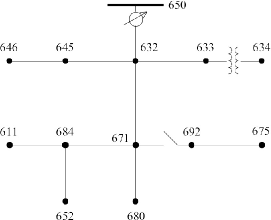
Figure 1: IEEE 13-feeder grid.

The power components of the known solution $(\hat{s},\hat{v})$ are given in Table I; voltage magnitudes are shown on Fig.3. For better expression, first re-number all the nodes. Then take the power injection $\hat{s}=\hat{p}+j\hat{q}$ with normalization base $5$MVA for Power and $4.16/\sqrt{3}=2.4$kV for Voltage (which is also the voltage of the slack bus).

TABLE I: Key Parameters

Index	$\hat{p}$(MW)	$\hat{q}$(Mvar)	$|\hat{s}|$(MVA)	e
$632\rightarrow 1$	-0.48	-0.32	0.58	1
$633\rightarrow 2$	1.28	0.96	1.60	1.05
$634\rightarrow 3$	-0.72	-0.48	0.87	0.95
$645\rightarrow 4$	0.96	0.8	1.25	1.03
$646\rightarrow 5$	-0.96	-0.8	1.25	1.01
$671\rightarrow 6$	0.64	0.48	0.80	1.05
$692\rightarrow 7$	-0.8	-0.48	0.93	0.97
$675\rightarrow 8$	0.64	0.48	0.80	1.04
$684\rightarrow 9$	-0.64	-0.48	0.80	0.99
$611\rightarrow 10$	0.32	0.24	0.4	1
$680\rightarrow 11$	-0.48	-0.32	0.58	1
$652\rightarrow 12$	0.32	0.24	0.4	1.05

VI-A Illustration of Main Theorem

Here, for illustration purpose, we apply Theorem 1 to test the candidate power injection $s$, where $s_{j}=\hat{s}_{j}e_{j}$ with $\hat{s}$ and $e$ as in Table I. The computed results are shown in Table II. It is easy to check that the conditions in Theorem 1 are satisfied. In contrast, note that $\xi(s)=0.5770>0.25$, i.e. the method and conditions given in [13] and [14] do not work in this case.

TABLE II: Computed Results

$\xi(\hat{s})$	$\xi(s-\hat{s})$	$\xi(s)$	$u_{min}$	$\rho$
0.5692	0.0164	0.5770	1.0050	0.0412

In Fig.2, the red circle is of radius $\rho=0.0412$ and represents $\mathcal{D}$ for one coordinate (here for instance, select Node 8).

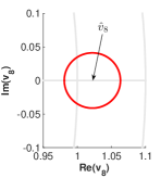
Figure 2: The domain $\mathcal{D}$ for one coordinate (Node 8).

In Fig.3, the solved voltage magnitudes are shown. In the same figure, the Newton-Raphson method is used for checking the result. It is well-observed that the method gives out the same solution as Newton-Raphson method. Actually, all the solution coordinates lie in the domain given by our theorem.

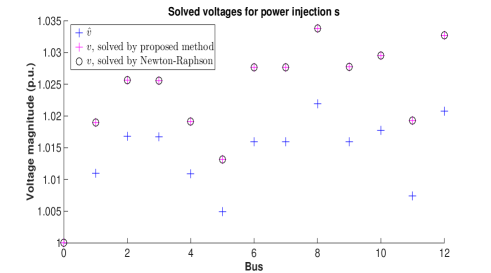
Figure 3: The voltages of power injection $\hat{s}$ and the computed voltages of power injection $s$.

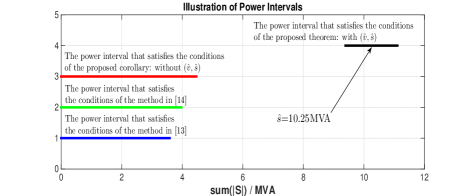
Figure 4: Intervals of power injection that satisfy the conditions of the proposed theorem, the proposed corollary, the method in [13] and the method in [14].

VI-B Continuation Power Flow analysis

In this subsection, we illustrate the range of power injections that are allowed and provided by our theorems, using “continuation power flow analysis” [23]. To this end, we do not take the candidate power injections $s$ from Table I but instead we scale them from $\hat{s}$. Specifically, let $s=\kappa\frac{\hat{s}}{{\parallel\hat{s}\parallel}_{1}}$ with $\kappa\in[0,\infty)$ MVA. In other words, the scaling factor $\kappa=\sum_{i=1}^{N}|s_{i}|$ is the sum of all apparent power injections. Then,

1) With ($\hat{v}$,$\hat{s}$): By applying the conditions of the proposed main theorem, the black interval is obtained in Fig.4. For all the summed power $\kappa$ in this interval, our conditions (9) and (10) are satisfied.

2) Without ($\hat{v}$,$\hat{s}$): Similarly, we can obtain the red interval by applying the conditions of the proposed corollary, the green interval by conditions of the method in [14], and the blue interval by conditions of the method in [13]. In this example, it is clear that the power interval provided by the proposed method (i.e., red interval) covers the power intervals provided by methods in [13] and [14] (i.e., green and blue intervals). In other words, the proposed method is (strictly) stronger than the methods in [13] and [14].

Remark 4.

Here, the $\Lambda$ for the method in [14] is chosen as suggested in [14] $\Lambda_{k}=1/\max_{h}|(W^{-1}Y_{LL}^{-1}\overline{W}^{-1})_{hk}|$.

VII Conclusion

We have provided explicit sufficient conditions that guarantee the existence and uniqueness of the feasible load-flow solution for distribution networks with generic topology modeled using their positive sequence equivalents. Our findings improve on all previously known results. The whole theory has been verified in IEEE benchmark grids.

The proposed method is of practical use, as it can easily be deployed in applications for microgrids and distribution networks that require solving load-flows in real time.

We plan to extend the results to more general three-phase networks in a subsequent paper.

Appendix A Invertibility of $Y_{LL}$

In circuit theory [24], there are already results on the invertibility of a full admittance matrix which includes the ground as one node. However, these results do not directly apply to $Y_{LL}$, which is only a sub-matrix of the nodal admittance matrix $Y$ that does not contain ground node. Having considered this fact, we give the proof of the invertibility of $Y_{LL}$ in this appendix. It is worth noticing that the proof does not require the network to be radial.

A-A Modeling and the Admittance Matrix

For the non-transformer connection (e.g., transmission lines) between node $i$ and $j$, the $2\times 2$ longitudinal admittance matrix is

$$\left[\begin{array}[]{cc}y_{ij}&-y_{ij}\\ -y_{ij}&y_{ij}\end{array}\right]$$

where $y_{ij}$ (equal to $y_{ji}$) is the summed admittance of all power lines going directly from node $i$ to node $j$.

For the transformer connection between node $i$ and $j$, without loss of generality, let node $i$ be connected to the primary side of this transformer and node $j$ be at the secondary side, the $2\times 2$ admittance matrix is given as

$$\left[\begin{array}[]{cc}y_{ij}^{t}&-y_{ij}^{t}K_{ij}^{-1}\\ -y_{ij}^{t}\overline{K_{ij}}^{-1}&y_{ij}^{t}|K_{ij}|^{-2}\end{array}\right]$$

where $y_{ij}^{t}$ is the equivalent aggregated admittance on the primary side, complex number $K_{ij}$ is the ratio. Reciprocally, we can denote $y_{ij}^{t}|K_{ij}|^{-2}$ by $y_{ji}^{t}$ which is the equivalent aggregated admittance on the secondary side, and $K_{ij}^{-1}$ by $K_{ji}$ which is the inverse ratio. Now, the terms in a general admittance matrix $Y$ including shunt elements can be explicitly written as

$$Y_{ij}=\left\{\begin{array}[]{ll}-y_{ij}&j\in\mathcal{N}(i)\\ -y_{ij}^{t}K_{ij}^{-1}&j\in\mathcal{N}^{t}(i)\\ 0&\textrm{otherwise}\end{array}\right.$$

and

$$Y_{ii}=y_{ii}^{shunt}+\sum_{j\in\mathcal{N}(i)}y_{ij}+\sum_{j\in\mathcal{N}^{t}(i)}y_{ij}^{t},$$

where $\mathcal{N}(i)$ is the set of nodes that have direct non-transformer connections with node $i$, and $\mathcal{N}^{t}(i)$ is the set of nodes that have direct transformer connections with node $i$. Here, $y_{ii}^{shunt}$ is the sum of shunt elements around node $i$.

A-B The Invertibility

If the grid is viewed as a graph where buses are vertices and power lines are edges, then a new graph can be generated by eliminating node 0. Suppose that the new graph has $c$ connected components, then by carefully re-numbering each node, $Y_{LL}$ can be written as a $c$-block diagonal matrix. In this way, $Y_{LL}$ is invertible iff all blocks are invertible. Thus, if we can show an arbitrary one of these components invertible, then the invertibility of $Y_{LL}$ is proved. Thus, without loss of generality, assume that the new graph itself be one connected component.

First, denote this undirected graph as $\mathcal{G}=(\mathcal{V},\mathcal{E})$. In addition, let $\mathcal{V}^{slack}\subseteq\mathcal{V}$ be the set of nodes that are originally connected to the slack bus; $\mathcal{G}^{t}=(\mathcal{V}^{t},\mathcal{E}^{t})$ be the subgraph that contains all the transformer edges and corresponding endpoints; $\mathcal{G}_{m}=(\mathcal{V}_{m},\mathcal{E}_{m})$, $m\in\{1,...,M\}$ be all the $M$ connected components in $(\mathcal{V},\mathcal{E}\setminus\mathcal{E}^{t})$.

Let $x$ be an N-by-1 vector such that $Y_{LL}x=0$, and for all $i\in\mathcal{V}^{slack}$ define

$$\tilde{y}_{i0}=\left\{\begin{array}[]{ll}y_{i0}&\textrm{non-transformer connection}\\ y_{i0}^{t}&\textrm{transformer connection}\end{array}\right.$$

Then, we have

$$\begin{split}&x^{H}Y_{LL}x=\sum_{i,j\in\mathcal{V}}\overline{x}_{i}(Y_{LL})_{ij}x_{j}\\ =&\sum_{i=1}^{N}\sum_{j:(i,j)\in\mathcal{E}\setminus\mathcal{E}^{t}}y_{ij}\overline{x}_{i}(x_{i}-x_{j})+\sum_{i=1}^{N}\sum_{j:(i,j)\in\mathcal{E}^{t}}y_{ij}^{t}\overline{x}_{i}(x_{i}-K_{ij}^{-1}x_{j})\\ &+\sum_{i\in\mathcal{V}^{slack}}\tilde{y}_{i0}|x_{i}|^{2}+\sum_{i\in\mathcal{V}}y_{ii}^{shunt}|x_{i}|^{2}\end{split}$$

For the first term, we have

$$\begin{split}&\sum_{i=1}^{N}\sum_{j:(i,j)\in\mathcal{E}\setminus\mathcal{E}^{t}}y_{ij}\overline{x}_{i}(x_{i}-x_{j})\\ =&\sum_{i=1}^{N}\sum_{j>i:(i,j)\in\mathcal{E}\setminus\mathcal{E}^{t}}y_{ij}\overline{x}_{i}(x_{i}-x_{j})+\sum_{i=1}^{N}\sum_{j<i:(i,j)\in\mathcal{E}\setminus\mathcal{E}^{t}}y_{ij}\overline{x}_{i}(x_{i}-x_{j})\\ =&\sum_{i=1}^{N}\sum_{j>i:(i,j)\in\mathcal{E}\setminus\mathcal{E}^{t}}y_{ij}\overline{x}_{i}(x_{i}-x_{j})+\sum_{i=1}^{N}\sum_{j>i:(i,j)\in\mathcal{E}\setminus\mathcal{E}^{t}}y_{ji}\overline{x}_{j}(x_{j}-x_{i})\\ =&\sum_{i=1}^{N}\sum_{j>i:(i,j)\in\mathcal{E}\setminus\mathcal{E}^{t}}\left(y_{ij}\overline{x}_{i}(x_{i}-x_{j})+y_{ij}\overline{x}_{j}(x_{j}-x_{i})\right)\\ =&\sum_{i<j:(i,j)\in\mathcal{E}\setminus\mathcal{E}^{t}}y_{ij}|x_{i}-x_{j}|^{2}\end{split}$$

Similarly, for the second term, we have

$$\begin{split}&\sum_{i=1}^{N}\sum_{j:(i,j)\in\mathcal{E}^{t}}y_{ij}^{t}\overline{x}_{i}(x_{i}-K_{ij}^{-1}x_{j})\\ =&\sum_{i=1}^{N}\sum_{j>i:(i,j)\in\mathcal{E}^{t}}y_{ij}^{t}\overline{x}_{i}(x_{i}-K_{ij}^{-1}x_{j})+\sum_{i=1}^{N}\sum_{j<i:(i,j)\in\mathcal{E}^{t}}y_{ij}^{t}\overline{x}_{i}(x_{i}-K_{ij}^{-1}x_{j})\\ =&\sum_{i=1}^{N}\sum_{j>i:(i,j)\in\mathcal{E}^{t}}y_{ij}^{t}\overline{x}_{i}(x_{i}-K_{ij}^{-1}x_{j})+\sum_{i=1}^{N}\sum_{j>i:(i,j)\in\mathcal{E}^{t}}y_{ji}^{t}\overline{x}_{j}(x_{j}-K_{ji}^{-1}x_{i})\\ =&\sum_{i=1}^{N}\sum_{j>i:(i,j)\in\mathcal{E}^{t}}(y_{ij}^{t}\overline{x}_{i}(x_{i}-K_{ij}^{-1}x_{j})+y_{ij}^{t}\overline{K}_{ij}^{-1}\overline{x}_{j}(K_{ij}^{-1}x_{j}-x_{i}))\\ =&\sum_{i<j:(i,j)\in\mathcal{E}^{t}}y_{ij}^{t}|x_{i}-K_{ij}^{-1}x_{j}|^{2}\end{split}$$

So that,

$$\begin{split}&x^{H}Y_{LL}x\\ =&\sum_{i<j:(i,j)\in\mathcal{E}\setminus\mathcal{E}^{t}}y_{ij}|x_{i}-x_{j}|^{2}+\sum_{i<j:(i,j)\in\mathcal{E}^{t}}y_{ij}^{t}|x_{i}-K_{ij}^{-1}x_{j}|^{2}\\ &+\sum_{i\in\mathcal{V}^{slack}}\tilde{y}_{i0}|x_{i}|^{2}+\sum_{i\in\mathcal{V}}y_{ii}^{shunt}|x_{i}|^{2}=0\end{split}$$

Since $\Re{\tilde{y}_{i0}}>0$ for all $i\in\mathcal{V}^{slack}$, $\Re{y_{ii}^{shunt}}$ non-negative for all $i\in\mathcal{V}$, and $\Re{y_{ij}},\Re{y_{ij}^{t}}>0$ for all $i,j$ s.t. $(i,j)\in\mathcal{E}$, we have

1. $x_{i}=0$ for all $i\in\mathcal{V}^{slack}$;

2. $x_{i}=x_{j}$ for all $i,j\in\mathcal{V}_{m}$ given any $m\in\{1,...,M\}$;

3. $x_{i}=K_{ij}^{-1}x_{j}$ for all $i,j$ s.t. $(i,j)\in\mathcal{E}^{t}.$

Because $\mathcal{G}$ is connected, it can be obtained that

• By above 1 and 2, there exists at least one $m$ s.t. $x_{i}=0$ for all $i\in\mathcal{V}_{m}$.

• By 2 and 3, the zero value will propagate throughout $\mathcal{G}$.

Thus, the vector $x$ must be a zero vector, which implies $Y_{LL}$ has a trivial null space and hence is invertible.

References

- [1] A. J. Korsak, “On the question of uniqueness of stable load-flow solutions,” IEEE Trans. on Power App. Syst., vol. PAS-91, pp. 1093–1100, May 1972.
- [2] B. K. Johnson, “Extraneous and false load flow solutions,” IEEE Trans. on Power App. Syst., vol. PAS-96, no. 2, pp. 524–534, Mar. 1977.
- [3] Y. Wang and W. Xu, “The existence of multiple power flow solutions in unbalanced three-phase circuits,” IEEE Trans. on Power Systems, vol. 18, no. 2, pp. 605–610, May 2003.
- [4] T. Del Carpio-Huayllas, D. Ramos, and R. Vasquez-Arnez, “Microgrid transition to islanded modes: conceptual background and simulation procedures aimed at assessing its dynamic performance,” in Proceedings of the 2012 IEEE PES Transmission and Distribution Conference and Exposition (T&D), Orlando, FL, 2012, pp. 1––6.
- [5] A. Bernstein, L. Reyes-Chamorro, J.-Y. Le Boudec, and M. Paolone, “Real-time control of microgrids with explicit power setpoints: unintentional islanding,” in PowerTech 2015, 2015.
- [6] A. Bernstein, L. Reyes-Chamorro, J.-Y. Le Boudec, and M. Paolone, “A composable method for real-time control of active distribution networks with explicit power setpoints. Part I: Framework,” Electric Power Systems Research, vol. 125, pp. 254 – 264, 2015.
- [7] J. Thorp, D. Schulz, and M. Ilic-Spong, “Reactive power-voltage problem: Conditions for the existence of solution and localized disturbance propagation,” Int. J. Electr. Power Energy Syst., vol. 8, pp. 66–76, Apr. 1986.
- [8] M. Ilic, “Network theoretic conditions for existence and uniqueness of steady state solutions to electric power circuits,” in ICSAS, San Diego, CA, 1992, pp. 2821––2828.
- [9] H.-D. Chiang and M. E. Baran, “On the existence and uniqueness of load flow solution for radial distribution power networks,” IEEE Trans. on Circuits and Systems, vol. 37, no. 3, pp. 410–416, Mar. 1990.
- [10] K. N. Miu and H.-D. Chiang, “Existence, uniqueness, and monotonic properties of the feasible power flow solution for radial three-phase distribution networks,” IEEE Trans. on Circuits and Systems, vol. 47, no. 10, pp. 1502–1514, Oct. 2000.
- [11] J. Meisel and R. D. Barnard, “Application of fixed-point techniques to load-flow studies,” IEEE Trans. on Power App. Syst., vol. PAS-89, no. 1, pp. 136–140, Jan. 1970.
- [12] A. C. Lisboa, L. S. M. Guedes, D. A. G. Vieira, and R. R. Saldanha, “A fast power flow method for radial networks with linear storage and no matrix inversions,” Int. J. Electr. Power Energy Syst., vol. 63, pp. 901–907, 2014.
- [13] S. Bolognani and S. Zampieri, “On the existence and linear approximation of the power flow solution in power distribution networks,” arXiv preprint arXiv:1403.5031, 2015.
- [14] S. Yu, H. D. Nguyen, and K. S. Turitsyn, “Simple certificate of solvability of power flow equations for distribution systems,” arXiv preprint arXiv:1503.01506, 2015.
- [15] T.-H. Chen, M.-S. Chen, K.-J. Hwang, P. Kotas, and E. A. Chebli, “Distribution system power flow analysis - a rigid approach,” IEEE Trans. on Power Deliv., vol. 6, no. 3, pp. 1146–1152, Jul. 1991.
- [16] H. M. Markowitz, “The elimination form of the inverse and its application to linear programming,” Management Sci., vol. 3, no. 3, pp. 255–269, Apr. 1957.
- [17] W. F. Tinney and J. W. Walker, “Direct solutions of sparse network equations by optimally ordered triangular factorization,” Proceedings of the IEEE, no. 55(11), pp. 1801––1809, Nov. 1967.
- [18] F. L. Alvarado, W. F. Tinney, and M. K. Enns, “Sparsity in large-scale network computation,” Advances in Electric Power and Energy Conversion System Dynamics and Control, vol. 41, pp. 207–272, 1991.
- [19] A. Quarteroni, R. Sacco, and F. Saleri, Numerical mathematics, 2nd ed., ser. 37. Springer, 2007.
- [20] A. Hjørungnes and D. Gesbert, “Complex-valued matrix differentiation: techniques and key results,” IEEE Trans. on Signal Processing, vol. 55, no. 6, pp. 2740–2746, Jun. 2007.
- [21] W. H. Kersting, “Radial distribution test feeders,” in IEEE PES Winter Meeting, vol. 2, Jan. 2001, pp. 908–912.
- [22] ——, “Radial distribution test feeders,” IEEE Trans. on Power Systems, vol. 6, no. 3, pp. 975–985, Aug. 1991.
- [23] F. Milano, Power system modelling and scripting. Springer, 2010.
- [24] C. A. Desoer and E. S. Kuh, Basic circuit theory. McGraw-Hill Education, 1969.