Quantum noise limit for force sensitivity of linear detectors

Abstract

We prove that the force sensitivity of the conventional optomechanical detector associated with the optical quadrature measurement of the output beam is lower bounded by the so-called ultimate quantum limit (UQL), i.e., the absolute value of the imaginary part of the inverse mechanical susceptibility. Through the linear response theory, we find that the force sensitivity of any linear detector is lower bounded by a generalized UQL, which might beat the usual UQL by properly tailoring the detector-oscillator interaction. We believe that our results open a new direction for improving the performance of high-sensitivity detection schemes.

Introduction.—Quantum noise is known to impose fundamental limits on high-sensitivity measurements qm ; cave . For a force measurement with an optomechanical detector cave ; clerk , the force is estimated from its effect on the position of a harmonic oscillator. The displacement of the oscillator is then read out by a probing laser beam. The force sensitivity of the measurement is limited by two types of quantum noise: the shot noise of the laser beam at the detection port and the radiation pressure backaction noise introduced by the oscillator clerk . An optimal tradeoff between these noises induces a lower bound for classical detection sensitivity, which is the so-called standard quantum limit (SQL) qm ; cave ; clerk .

However, the SQL itself is not a fundamental quantum limit. Various schemes to overcome the SQL in force measurements have been proposed, such as frequency dependent squeezing (FDS) of the input beam fds ; uql , cavity detuning (CD) cd , variational measurement (VM) vm , coherent quantum noise cancelation (CQNC) cqnc , etc. More importantly, an immediate question is to find out the fundamental quantum limit for the force sensitivity. In this letter, we aim to answer this question. For the mentioned schemes that beat the SQL, we find that the corresponding force sensitivities are lower bounded by the so-called UQL uql ; cd . It is related to the dissipation mechanism of the oscillator, via the absolute value of the imaginary part of the inverse mechanical susceptibility. Through the linear response theory, we prove that the force sensitivity of any linear detector is lower bounded by a generalized UQL, which can be achieved by properly tailoring the detector so as to overcome the usual UQL. This lower bound also holds for the cases with coherent quantum control and/or quantum feedback cqc ; qfb . The purpose of this letter is to provide a criterion for the sensitivity limit, just as the Heisenberg limit in quantum optical phase estimation hl , and stimulate some promising approaches for improving the performance of high-sensitivity detection schemes.

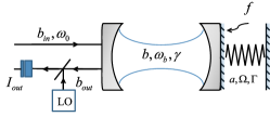
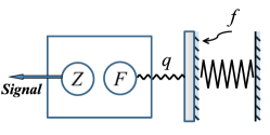
Figure 1: Schematics of the conventional optomechanical detector (a) and the generic force detector (b). (a) The output current $I_{out}$ of the photodiode is modulated by the local oscillator phase. (b) The detector’s input and output operators $F$, $Z$ are coupled to the oscillator and the readout apparatus, respectively.

Optomechanical detector.—The optomechanical detector consists of a high quality Fabry-Perot cavity, with a fixed transmissive mirror in front of the cavity, and a moveable, perfectly reflecting mirror at the back (see Fig. 1a). The cavity is in thermal equilibrium with the radiation, and is fed with a driving laser. We aim to estimate a classical force acting on the moveable mirror of cavity, for example, the passing of a gravitational wave gwave . In the rotating frame at the driving frequency $\omega_{0}$ of the input laser, the system is described by the Hamiltonian ($\hbar=1$)

$$H=H_{m}+H_{o}-g_{om}x(b^{\dagger}b-\langle b^{\dagger}b\rangle)+H_{dr},$$ (1)

where $H_{m}=\Omega a^{\dagger}a-xf(t)$ is the mechanical oscillator under the classical force $f(t)$, and $H_{o}=\Delta b^{\dagger}b$ is the cavity with the resonance frequency $\omega_{b}$ at the equilibrium position $x=0$ in the presence of the mean radiation pressure and the cavity detuning $\Delta=\omega_{b}-\omega_{0}$. The third term captures optomechanical interaction with the coupling strength $g_{om}$. The last term $H_{dr}=i\sqrt{\gamma}(\beta_{in}b^{\dagger}-h.c.)$ is the laser driving Hamiltonian. Taking into account the thermal noises, the equations of motion are given by the quantum Langevin equations qop ,

$$\dot{a} = i[H,a]-\frac{\Gamma}{2}a+\sqrt{\Gamma}a_{in},$$

$$\dot{b} = i[H,b]-\frac{\gamma}{2}b+\sqrt{\gamma}b_{in},$$ (2)

where $\Gamma(\gamma)$ and $a_{in}(b_{in})$ are the decay rate and thermal noise operator for the oscillator (cavity), respectively. The noise correlators are $\langle a_{in}(t)a_{in}^{\dagger}(t^{\prime})\rangle=(n_{th}+1)\delta(t-t^{\prime})$ and $\langle b_{in}(t)b_{in}^{\dagger}(t^{\prime})\rangle=\delta(t-t^{\prime})$, where $n_{th}$ is the thermal occupancy of the mechanical reservoir.

Under the condition of strong laser driving, we can linearize the system dynamics by splitting $a\to\langle a\rangle+a$ and $b\to\langle b\rangle+b$, where $\langle a\rangle=0$ and $\langle b\rangle=\beta$ are the mean field values. The linearized equation of motion is obtained by neglecting the nonlinear terms in Eq. (2),

$$\dot{\mathbf{x}}={\mathbf{A}\mathbf{x}}+\mathbf{w},$$ (3)

where the variables $\mathbf{x}=(x,p,b_{1},b_{2})^{T}$ with $a=(x+ip)/\sqrt{2}$ and $b=(b_{1}+ib_{2})/\sqrt{2}$, the input $\mathbf{w}=(\sqrt{\Gamma}x_{in},f+\sqrt{\Gamma}p_{in},\sqrt{\gamma}b_{1}^{in},\sqrt{\gamma}b_{2}^{in})^{T}$, and the matrix

$$\mathbf{A}=\left(\begin{matrix}-{\Gamma\over 2}&\Omega&0&0\\ -\Omega&-{\Gamma\over 2}&g&0\\ 0&0&-{\gamma\over 2}&\Delta\\ g&0&-\Delta&-{\gamma\over 2}\end{matrix}\right),$$ (4)

where $g=\sqrt{2}\beta g_{om}$ is the effective optomechanical coupling strength.

The classical force is estimated from the output current $I_{out}$ of a photodiode that is linearly proportional to a certain optical quadrature of the output field, $I_{out}\propto y\equiv b_{1}^{out}\sin\phi+b_{2}^{out}\cos\phi$, where $\phi$ is the adjustable readout quadrature angle via the local oscillator phase. The output vector $\mathbf{b}_{out}=(b_{1},b_{2})^{T}_{out}$ in the frequency domain, neglecting the intrinsic mechanical noise of the oscillator, is determined by the input-output relation:

$$\mathbf{b}_{out}={\bf M}\mathbf{b}_{in}+\mathbf{v}f,$$ (5)

where $\bf M$ is the $2\times 2$ transfer matrix, and ${\bf v}=(v_{1},v_{2})^{T}$. Putting Eq. (5) into the expression of $y$, we get $y=\mathbf{d}^{T}_{\phi}\mathbf{b}_{out}=\mathbf{d}^{T}_{\phi}{\bf M}{\bf b}_{in}+\mathbf{d}^{T}_{\phi}{\bf v}f$ with ${\bf d}=(\sin\phi,\cos\phi)^{T}$. The first term represents the quantum noise, and the second term is the output response to the classical force. The normalized quadrature gives an unbias estimator $\hat{f}$ of $f$, $\hat{f}={y}/(\mathbf{d}^{T}_{\phi}{\bf v})=f+f_{add}$, where $f_{add}=\mathbf{d}^{T}_{\phi}{\bf M}{\bf b}_{in}/(\mathbf{d}^{T}_{\phi}{\bf v})$ is the added noise. The force sensitivity is quantified by the power density of the added noise

$$S_{f}\delta(\omega-\omega^{\prime})=\langle f_{add}(\omega)f^{\dagger}_{add}(\omega^{\prime})+f^{\dagger}_{add}(\omega^{\prime})f_{add}(\omega)\rangle/2.$$ (6)

It gives $S_{f}={\mathbf{d}^{T}_{\phi}{\bf M}{\bf S}{\bf M}^{\dagger}\mathbf{d}_{\phi}}/{|\mathbf{d}^{T}_{\phi}{\bf v}|^{2}}$, where the power density matrix $\bf S$ for the quadratures $b_{1}^{in}$ and $b_{2}^{in}$ is defined by $S_{XY}(\omega)\delta(\omega-\omega^{\prime})=\langle X(\omega)Y^{\dagger}(\omega^{\prime})+Y^{\dagger}(\omega^{\prime})X(\omega)\rangle/2$.

For a resonant cavity ($\Delta=0$), the added noise is supple

$$f_{add}=\frac{\xi b_{1}^{in}+b_{2}^{in}}{g\sqrt{\gamma}\chi_{a}\chi_{b}^{*}}+g\sqrt{\gamma}\chi_{b}b_{1}^{in},$$ (7)

where $\chi_{a}={\Omega}\left[{(\Gamma/2-i\omega)^{2}+\Omega^{2}}\right]^{-1}$, $\chi_{b}=\left({\gamma/2-i\omega}\right)^{-1}$, and $\xi=\tan\phi$. Here the first term is the shot noise at the detection port, and the second term is the backaction noise from the oscillator due to radiation pressure. For non-squeezed coherent input laser, ${\bf S}={\bf I}/2$. Assuming $\phi=\xi=0$, Eq. (7) gives rise to

$$S_{f}=\frac{1}{2}\left({g^{2}\gamma}|\chi_{b}|^{2}+\frac{1}{g^{2}\gamma|\chi_{a}|^{2}|\chi_{b}|^{2}}\right)\geq\frac{1}{|\chi_{a}|},$$ (8)

where the inequality $a+b\geq 2\sqrt{|ab|}$ has been used. The minimal sensitivity is achieved when the backaction noise and shot noise are balanced, known as the SQL for the detector sensitivity qm ; cave ; clerk . However, the SQL can be overcome by several schemes.

Schemes to beat the SQL.—A simple scheme to beat the SQL is just varying the readout quadrature angle ($\phi\neq 0$) vm . It introduces an extra $\xi$-dependent shot noise to destructively interfere with the original backaction noise and to give a better sensitivity. From Eq. (7), we have in terms of $\bar{\chi}_{a}=1/{\chi}_{a}=\bar{\chi}_{a}^{R}+i\bar{\chi}_{a}^{I}$,

$$S_{f} = \xi\bar{\chi}_{a}^{R}+\frac{1}{2}\left({g^{2}\gamma}|\chi_{b}|^{2}+\frac{1+\xi^{2}}{g^{2}\gamma|\chi_{a}|^{2}|\chi_{b}|^{2}}\right)$$ (9)

$$\geq \xi\bar{\chi}_{a}^{R}+\frac{\sqrt{1+\xi^{2}}}{|\chi_{a}|}\geq|\bar{\chi}_{a}^{I}|,$$

where the inequalities $a+b\geq 2\sqrt{|ab|}$ and $ax+\sqrt{(1+x^{2})(a^{2}+b^{2})}\geq|b|$ have been used. This lower bound for force sensitivity is the known UQL in Refs. cd ; uql , which has also been discussed in the limits of weak coupling and high power gain in Ref. clerk .

Another scheme to beat the SQL in Ref. fds is to use a frequency dependent squeezed input laser with the elements, $S_{11}=u$, $S_{22}=v$, and $S_{12}=S_{21}=w$. The interference between the backaction noise and the shot noise due to the correlation between $b_{1}^{in}$ and $b_{2}^{in}$ ($w\neq 0$) could give rise to certain negative terms in the $S_{f}$, and thus surpass the SQL. For a coupled VM-FDS scheme, Eq. (7) gives

$$S_{f} = 2(\xi u+w)\bar{\chi}_{a}^{R}+{g^{2}\gamma|\chi_{b}|^{2}}u+\frac{\xi^{2}u+2\xi w+v}{g^{2}\gamma|\chi_{a}|^{2}|\chi_{b}|^{2}}$$ (10)

$$\geq 2(\xi u+w)\bar{\chi}_{a}^{R}+\frac{2}{|\chi_{a}|}\sqrt{u(\xi^{2}u+2\xi w+v)}$$

$$\geq h\bar{\chi}_{a}^{R}+\frac{\sqrt{1+h^{2}}}{|\chi_{a}|}\geq|\bar{\chi}_{a}^{I}|,\quad h=2(\xi u+w),$$

where the inequalities $a+b\geq 2\sqrt{|ab|}$, $uv-w^{2}\geq{1/4}$, and $ax+\sqrt{(1+x^{2})(a^{2}+b^{2})}\geq|b|$ have been used. In Ref. cd , a nonzero cavity detuning ($\Delta\neq 0$) is invoked, which simultaneously modifies the backaction noise and the shot noise, to beat the SQL. As shown in Fig. 2a, the UQL sets a lower bound to all the above schemes. Remarkably, the force sensitivity for a combined VM-FDS-CD scheme is also lower bounded by the UQL supple .

Finally, we show that the CQNC scheme cqnc that could beat the SQL still satisfies the UQL. In the CQNC scheme, an additional ancillary cavity of mode $c(t)=(c_{1}+ic_{2})/\sqrt{2}$ fed with the vacuum is introduced, and the following Hamiltonian is assumed:

$$H_{c}=-\Omega c^{\dagger}c-gb_{1}c_{1}.$$ (11)

The ancilla works effectively as a negative-mass oscillator, and its coupling with the main cavity can be realized via a beam-splitter and a nondegenerate optical parametric amplifier. Considering the intrinsic mechanical and cavity noises, the dynamics of the system is also governed by Eq.(3), where the variables $\mathbf{x}=(x,p,b_{1},b_{2},c_{1},c_{2})^{T}$, the input $\mathbf{w}=(\sqrt{\Gamma}x_{in},f+\sqrt{\Gamma}p_{in},\sqrt{\gamma}b_{1}^{in},\sqrt{\gamma}b_{2}^{in},\sqrt{\Gamma}c_{1}^{in},\sqrt{\Gamma}c_{2}^{in})^{T}$, and the matrix $\mathbf{A}$ is given in supple . Based on the output photoncurrent at readout angle $\phi$, the added noise takes

$$f_{add}={\xi b_{1}^{in}+b_{2}^{in}\over g\sqrt{\gamma}\chi_{a}\chi_{b}^{*}}+\mathcal{F}_{c},$$ (12)

where $\mathcal{F}_{c}={\sqrt{\Gamma}}\left[c_{1}^{in}(\Gamma/2-i\omega)/\Omega-c_{2}^{in}\right]$ is the intrinsic noise from the ancillary cavity. It can be seen that the backaction noise from the main cavity was canceled out. For sufficiently large pump $g\gg 1$, the shot noise from the main cavity can be made insignificant with respect to $\mathcal{F}_{c}$. The detector sensitivity is essentially given by the power density of $\mathcal{F}_{c}$,

$$S_{f}\approx\frac{\Gamma}{2\Omega^{2}}\bigg{(}\omega^{2}+\Omega^{2}+{\Gamma^{2}\over 4}\bigg{)}\geq{\omega\Gamma\over\Omega}=|\bar{\chi}_{a}^{I}|,$$ (13)

namely, the UQL.

Optimal force sensitivity for linear response detector.— For the conventional optomechanical detector, the above results suggest that the UQL might be true for any detection scheme, such as the cases in Ref. more ; pt . To determine this conjecture, we consider some physical system as a generic linear response detector (see Fig. 1b). The detector is described by some unspecified Hamiltonian $H_{d}$, and has both an input operator, represented by an operator $F$, and an output operator, represented by an operator $\mathcal{Z}$. The input operator $F$ is coupled with the mechanical oscillator via the interaction Hamiltonian, $H_{int}=-gFq$, where the oscillator operator $q$ is not necessarily the position operator $x$, as long as it carries the input signal. The output operator $\mathcal{Z}$ (e.g., the output optical quadrature $y$) is related to the readout quantity at the output of the detector (e.g., the output current $I_{out}$ of the photodiode), from which the classical force is estimated.

The total Hamiltonian is given by $H=H_{m}+H_{d}+H_{int}$. Treating $H_{int}$ as the perturbation, an arbitrary operator $O$ in the Heisenberg picture is obtained by

$$O(t)=\mathcal{U}^{\dagger}O_{0}(t)\mathcal{U},\quad\mathcal{U}(t)=\mathcal{T}e^{-i\int_{-\infty}^{t}H^{0}_{int}(t)dt},$$ (14)

where $O_{0}(t)$ denotes the operator in the interaction picture, and the symbol $\mathcal{T}$ means the time-ordered product. For the linear operators $q$, $F$, and $Z$ (with the c-number commutators), Eq. (14) gives supple

$$q(\omega) = q_{0}(\omega)+\chi_{qx}(\omega)f(\omega)+g\chi_{qq}(\omega)F(\omega),$$

$$F(\omega) = F_{0}(\omega)+g\chi_{F\!\!\!\ F}(\omega)q(\omega),$$

$$Z(\omega) = Z_{0}(\omega)+gq(\omega),$$ (15)

where $Z$ is the rescaled output operator via $\mathcal{Z}(\omega)=\chi_{\mathcal{Z}\!\!\!\ F}(\omega)Z(\omega)$. The susceptibility $\chi_{XY}$ is defined via the c-number commutator, $\chi_{X\!\!\!\ Y}(t)=i\theta(t)[X(t),Y(0)]$.

Solving the first two equations and substituting into the third one of Eq. (15), we have the output operator in terms of the unperturbed operators,

$$Z(\omega)=Z_{0}+g{q_{0}+\chi_{qx}f+g\chi_{qq}F_{0}\over 1-g^{2}\chi_{qq}\chi_{F\!\!\!\ F}}.$$ (16)

The normalization of $Z$ gives the estimator $\hat{f}$ of $f$,

$$\hat{f}=f+\bar{\chi}_{qx}(q_{0}+G_{F}F_{0}+G_{Z}Z_{0})=f+f_{add},$$ (17)

where $G_{F}=g\chi_{qq}$ and $G_{Z}=(1-g^{2}\chi_{qq}\chi_{F\!\!\!\ F})/g$. The $F_{0}$-term represents the backaction noise from the oscillator, while the $Z_{0}$-term is the shot noise at the output. Neglecting the intrinsic mechanical noise $\propto q_{0}$, the scaled power density $S^{\prime}_{f}=S_{f}|\chi_{qx}|^{2}$ takes $S^{\prime}_{f}=|G_{F}|^{2}S_{F\!\!\!\ F}+|G_{Z}|^{2}S_{Z\!\!\!\ Z}+(G_{F}G_{Z}^{*}S^{*}_{Z\!\!\!\ F}+G_{F}^{*}G_{Z}S_{Z\!\!\!\ F})$, where the relation $S_{F\!\!\!\ Z}=S^{*}_{Z\!\!\!\ F}$ has been used. The optimization of $S^{\prime}_{f}$ over the coupling strength $g$ gives

$$S^{\prime}_{f} \geq 2(A\chi^{R}_{qq}-B\chi^{I}_{qq})+|\chi_{qq}|\big{[}S_{Z\!\!\!\ Z}(S_{F\!\!\!\ F}+|\chi_{F\!\!\!\ F}|^{2}S_{Z\!\!\!\ Z}$$ (18)

$$-2\chi^{R}_{F\!\!\!\ F}S^{R}_{Z\!\!\!\ F}+2\chi^{I}_{F\!\!\!\ F}S^{I}_{Z\!\!\!\ F})\big{]}^{1/2},$$

where $A=-\chi^{R}_{F\!\!\!\ F}S_{Z\!\!\!\ Z}+S^{R}_{Z\!\!\!\ F}$ and $B=\chi^{I}_{F\!\!\!\ F}S_{Z\!\!\!\ Z}+S^{I}_{Z\!\!\!\ F}$.

To proceed further, we must at least require $[\mathcal{Z}(t),\mathcal{Z}(t^{\prime})]=[\mathcal{Z}_{0}(t),\mathcal{Z}_{0}(t^{\prime})]=0$ at all times, in order for $\mathcal{Z}(t)$ and $\mathcal{Z}_{0}(t)$ to represent experimental data string. It immediately implies that $\chi_{\mathcal{Z}\!\!\!\ \mathcal{Z}}(\omega)=0$. Also, the causality principle imposes that the output $\mathcal{Z}_{0}(t)$ should not depend on the input $F_{0}(t^{\prime})$ for $t<t^{\prime}$, and therefore $\chi_{F\!\!\!\ \mathcal{Z}}(\omega)=0$. Furthermore, $F$ and $Z$ should satisfy the uncertainty relation supple ,

$$S_{F\!\!\!\ F}S_{Z\!\!\!\ Z}\geq|S_{Z\!\!\!\ F}|^{2}+|B|+1/4.$$ (19)

Putting Eq. (19) into (18), we obtain

$$S^{\prime}_{f} \geq 2(A\chi^{R}_{qq}-B\chi^{I}_{qq})+2|\chi_{qq}|\sqrt{A^{2}+(|B|+1/2)^{2}}$$ (20)

$$\geq -2B\chi^{I}_{qq}+2(|B|+1/2)|\chi^{I}_{qq}|\geq|\chi^{I}_{qq}|,$$

where the inequalities $a_{1}x_{1}+\sqrt{(a_{1}^{2}+a_{2}^{2})(x_{1}^{2}+x_{2}^{2})}\geq|a_{2}x_{2}|$ and $|a|\geq a$ have been applied. The resulting force sensitivity is

$$S_{f}\geq{|\chi^{I}_{qq}|}/{|\chi_{qx}|^{2}},$$ (21)

which is the main result of this letter. It can be viewed as a generalized UQL. For the optomechanical detector, we have $q=x$, $F=b_{1}$, $\mathcal{Z}=y$, $\chi_{qx}=\chi_{qq}=\chi_{a}$, and thus the usual UQL for the detector sensitivity. As an example, we could conclude that the sensitivity with a PT-symmetric cavity near the PT-phase transition pt can not be enhanced below the usual UQL, because therein the optomechanical interaction is of the form $-gxF$.

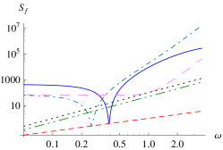
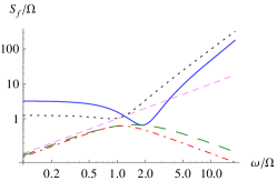
Figure 2: Plot of the force sensitivity versus the detection frequency. (a) Solid line: CD scheme ($\Delta=-7$); dot-dashed line: VM scheme ($\xi=20$); long-dashed line: the standard detection scheme; double-dot-dashed line: CQNC scheme; dotted line: the SQL; dashed line: the UQL. Here the system parameters are $\mathbf{S}=\mathbf{I}/2$, $\gamma=3$, $\Gamma=\Omega=0.01$, and $g=-10$. (b) Solid line: the toy optomechanical detector; long-dashed line: the generalized UQL ($q=x+p$); dashed line: the usual UQL ($q=x$); dotted line: the SQL; dot-dashed line: the optimal UQL. Here the system parameters are $\mathbf{S}=\mathbf{I}/2$, $\gamma=100\Omega$, $\Gamma=\Omega$, $g=5\Omega$, and $\xi=0$.

On the other hand, if the detector is coupled with the oscillator via a certain $q\neq x$, the lower bound in Eq. (21) might be achieved by tuning the detector structure and even beat the usual UQL. It can be understood that the backaction noise and the shot noise are modified with more freedoms to fulfill a destructive interference in the $S_{f}$. As an example, we devise a toy optomechanical detector. The cavity-oscillator interaction is supposed to be $H_{int}=-g(x+p)(b_{1}+b_{2})$. The matrix $\mathbf{A}$ becomes

$$\mathbf{A}=\left(\begin{matrix}-{\Gamma\over 2}&\Omega&-g&-g\\ -\Omega&-{\Gamma\over 2}&g&g\\ -g&-g&-{\gamma\over 2}&0\\ g&g&0&-{\gamma\over 2}\end{matrix}\right),$$ (22)

which satisfies the stability condition since the eigenvalues of $\mathbf{A}$ are ($-{\gamma\over 2}$, $-{\gamma\over 2}$, $-{\Gamma\over 2}+i\Omega$, $-{\Gamma\over 2}-i\Omega$). This type of coupling might be realized in one-dimensional superconducting stripline resonators bu . Based on the measurement of $y$, the power density of the added noise can be calculated. The numerical result is plotted in Fig. 2b. It shows that the generalized UQL

$$S_{f}\geq 2\left[\bigg{(}1+\frac{\Gamma}{2\Omega}\bigg{)}^{2}+\frac{\omega^{2}}{\Omega^{2}}\right]^{-1}{\omega\Gamma\over\Omega}$$ (23)

is achievable at a certain frequency and beats the usual UQL. Eq. (23) is obtained from Eq. (21) with the susceptibilities $\chi_{qq}=2\chi_{a}$ and $\chi_{qx}=\left[1+(\Gamma/2-i\omega)/\Omega\right]\chi_{a}$. Moreover, by varying over all possible linear coupling operator $q=x+\eta p$ in Eq. (21), we get the optimal UQL

$$S_{f} \geq {\Gamma\over 2\omega\Omega}\bigg{[}\frac{\Gamma^{2}}{4}+\omega^{2}+\Omega^{2}$$ (24)

$$-\sqrt{\bigg{(}\frac{\Gamma^{2}}{4}+\omega^{2}-\Omega^{2}\bigg{)}^{2}+\Gamma^{2}\Omega^{2}}\bigg{]},$$

which approaches $\Gamma\Omega/\omega$ for $\omega\gg\Omega$, and is different from the usual UQL scaling as $\omega\Gamma/\Omega$.

Obviously, the above result has incorporated the effect of coherent quantum control cqc , such as the CNQC scheme. As for the direct quantum feedback control qfb , the output signal is fed back to the system for changing the dynamical evolution. It introduces an additional term to the equation of motion for a generic operator $O$, $\dot{O}_{fb}(t)=i\lambda\mathcal{Z}(t)[\mathcal{P},O]$, where $\lambda$ is the feedback gain, $\mathcal{P}(t)$ is the control operator. Within this formalism, the generalized UQL for force sensitivity still holds supple .

Conclusion.—We have shown that the force sensitivity of the standard optomechanical detector associated with the optical quadrature measurement of the output field is lower bounded by the usual UQL. By the linear response theory, we have also found that the force sensitivity of any linear detector is lower bounded by the generalized UQL, which can beat the usual UQL by appropriately tailoring the detector. A toy optomechanical detector is devised to beat the usual UQL. We believe that this study provides a criterion for the sensitivity limit, just as the Heisenberg limit in quantum optical phase estimation, and even gives a promising approach for improving the performance of high-sensitivity detection schemes.

YG acknowledges the support from NSFC Grant No. 11304265. HH and HZ acknowledge financial support from the CRF scheme (CUHK1/CRF/12G), the ITF scheme (GHP/014/13SZ), and the AoE scheme (AoE/P-02/12) from the Research Grants Council (RGC) of Hong Kong Special Administrative Region, China.

Supplemental Materials

.1 Optomechanical detector

The equation of motion of the optomechanical system is given by Eq. (3). The explicit form takes

$$\dot{x} = -\frac{\Gamma}{2}x+\Omega p+\sqrt{\Gamma}x_{in},$$

$$\dot{p} = -\Omega x-\frac{\Gamma}{2}p+g_{om}(b^{\dagger}b-\langle b^{\dagger}b\rangle)+f+\sqrt{\Gamma}p_{in},$$

$$\dot{b} = -i\Delta b-\frac{\gamma}{2}b+ig_{om}xb+\sqrt{\gamma}(\beta_{in}+b_{in}).$$ (25)

Then we find the steady mean state to be $\langle x\rangle=\langle p\rangle=0$ and $\langle b\rangle=\beta=\sqrt{\gamma}\beta_{in}/({\gamma/2}+i\Delta)$. For convenience, we have chosen $\beta$ as real by adjusting the driving field $\beta_{in}$. The linearization of Eq. (25) around this steady state gives Eq. (3). The stability of this linearized system is guaranteed by the requirement that the real part of all the eigenvalues of $\mathbf{A}$ must be nonpositive. For the stationary state, the Fourier transform of Eq. (3)

$$-i\omega{\bf x}={\bf A}{\bf x}+{\bf w}$$ (26)

yields the solution ${\bf x}=-({\bf A}+i\omega{\bf I})^{-1}{\bf w}$. The output field is obtained by the input-output relation $b_{out}=\sqrt{\kappa}b-b_{in}$. Neglecting the intrinsic mechanical noises due to $x_{in}$ and $p_{in}$, we get Eq. (5), where ${\bf M}={\bf M}_{shot}+{\bf M}_{back}$,

$${\bf M}_{shot} = -{\bf I}+\gamma\left(\begin{matrix}\chi_{r}&\chi_{\Delta}\\ -\chi_{\Delta}&\chi_{r}\end{matrix}\right),$$

$${\bf M}_{back} = {g^{2}\gamma\chi_{a}\over 1-g^{2}\chi_{a}\chi_{\Delta}}\left(\begin{matrix}\chi_{r}\chi_{\Delta}&\chi_{\Delta}^{2}\\ \chi_{r}^{2}&\chi_{r}\chi_{\Delta}\end{matrix}\right),$$

$${\bf v} = {g\sqrt{\gamma}\chi_{a}\over 1-g^{2}\chi_{a}\chi_{\Delta}}\left(\begin{matrix}\chi_{\Delta}\\ \chi_{r}\end{matrix}\right).$$ (27)

Here we have separated the output field into the shot noise term, i.e., the output field without the interaction ($g=0$), and the backaction noise term depending on $g$. The quantities $\chi_{r(\Delta)}$ are defined by

$$\chi_{r} = \frac{r}{r^{2}+\Delta^{2}},$$

$$\chi_{\Delta} = \frac{\Delta}{r^{2}+\Delta^{2}}$$ (28)

with $r=\gamma/2-i\omega$. The added noise $f_{add}$ can then be written as

$$f_{add}=\mathbf{d}^{T}_{\phi}{\bf M}_{shot}{\bf b}_{in}/(\mathbf{d}^{T}_{\phi}{\bf v})+\mathbf{d}^{T}_{\phi}{\bf M}_{back}{\bf b}_{in}/(\mathbf{d}^{T}_{\phi}{\bf v}).$$ (29)

For a resonant cavity ($\Delta=0$), $\chi_{r}=\chi_{b}$ and $\chi_{\Delta}=0$, we get

$${\bf M}_{shot} = e^{i\theta}{\bf I},\quad e^{i\theta}=\chi_{b}/\chi_{b}^{*},$$

$${\bf M}_{back} = g^{2}\gamma\chi_{a}\chi_{b}^{2}\left(\begin{matrix}0&0\\ 1&0\end{matrix}\right),$$

$${\bf v} = g\sqrt{\gamma}\chi_{a}\chi_{b}\left(\begin{matrix}0\\ 1\end{matrix}\right).$$ (30)

Substituting them into Eq. (29) gives the added noise in Eq. (7).

To prove the UQL for the combined VM-FDS-CD scheme, we note that $f_{add}$ obtained from Eq. (29) takes the form

$$f_{add}={\bar{\chi}_{a}D+E\over C}b_{1}^{in}+{\bar{\chi}_{a}X+Y\over C}b_{2}^{in},$$ (31)

where

$$D = \xi(|r|^{2}-\Delta^{2})-\gamma\Delta,$$

$$E = g^{2}(\gamma+\xi\Delta),$$

$$X = |r|^{2}-\Delta^{2}+\xi\gamma\Delta,$$

$$Y = g^{2}\Delta,$$

$$C = g\sqrt{\gamma}(r+\xi\Delta).$$ (32)

Using the input density matrix $\bf S$ (with elements $S_{11}=u$, $S_{22}=v$, and $S_{12}=S_{21}=w$), the sensitivity is given by

$$S_{f}=2\bar{\chi}_{a}^{R}H+K+|\bar{\chi}_{a}|^{2}L$$

$$\geq 2\bar{\chi}_{a}^{R}H+2|\bar{\chi}_{a}|\sqrt{KL},$$ (33)

where

$$H = (DEu+EXw+DYw+XYv)/|C|^{2},$$

$$K = (E^{2}u+2EYw+Y^{2}v)/|C|^{2},$$

$$L = (D^{2}u+2DXw+X^{2}v)/|C|^{2}.$$ (34)

It is simple to check the identities

$$KL-H^{2} = (uv-w^{2})(EX-DY)^{2}/|C|^{2},$$

$$(EX-DY)^{2} = |C|^{2}.$$ (35)

Noting the inequality $uv-w^{2}\geq 1/4$, we finally have

$$S_{f}\geq 2\bar{\chi}_{a}^{R}H+2|\bar{\chi}_{a}|\sqrt{H^{2}+1/4}\geq|\bar{\chi}_{a}^{I}|,$$ (36)

which is the UQL for the optomechanical detector. For a pure squeezed input driving, we have

$$u = \cosh 2s-\sinh 2s\cos 2\varphi,$$

$$v = \cosh 2s+\sinh 2s\cos 2\varphi,$$

$$w = -\sinh 2s\sin 2\varphi,$$ (37)

and $uv-w^{2}=1/4$, where $s$ is called the squeezing factor and $\varphi$ is the squeezing angle.

For the CQNC scheme, the ancillary Hamiltonian can be realized by a beam splitter described by the interaction form $-g(bc^{\dagger}+b^{\dagger}c)/\sqrt{2}$ plus a non degenerate optical parameter amplifier described by the interaction term $-g(e^{-2i\omega_{0}t}b^{\dagger}c^{\dagger}+e^{2i\omega_{0}t}bc)/\sqrt{2}$. In the rotating frame at frequency $\omega_{0}$ ($b\to e^{-i\omega_{0}t}b$ and $c\to e^{-i\omega_{0}t}c$), the relevant Hamiltonian becomes $H_{c}=(\omega_{c}-\omega_{0})c^{\dagger}c-gb_{1}c_{1}$. Choosing the detuning $\omega_{c}-\omega_{0}=-\Omega$, we get the Hamiltonian in Eq. (11). So the ancilla works as a negative mass oscillator in order to cancel the backaction noise from the main cavity. The resulting matrix for the resonant case ($\Delta=0$) is

$$\mathbf{A}=\left(\begin{matrix}-{\Gamma\over 2}&\Omega&0&0&0&0\\ -\Omega&-{\Gamma\over 2}&g&0&0&0\\ 0&0&-{\gamma\over 2}&0&0&0\\ g&0&0&-{\gamma\over 2}&g&0\\ 0&0&0&0&-{\Gamma\over 2}&-\Omega\\ 0&0&g&0&\Omega&-{\Gamma\over 2}\end{matrix}\right),$$ (38)

where the decay rate of the ancilla is assumed to be the same as the mechanical oscillator. The final output field is given by

$${\bf b}_{out}=e^{i\theta}{\bf b}_{in}+g\sqrt{\gamma}\chi_{a}\chi_{b}\left(\begin{matrix}0\\ 1\end{matrix}\right)(f+\mathcal{F}_{c}),$$ (39)

where the backaction noise from the main cavity vanishes, due to the coherent cancelation, at the cost of an extra noise $\mathcal{F}_{c}$ from the ancillary cavity.

.2 Linear system and spectral uncertainty relations

The general linear system we described in the main text is $H=H_{m}+H_{d}+H_{int}$ with $H_{int}=-gFq$. The operator in the Heisenberg picture is given by Eq. (14), where $H_{int}^{0}=-gF_{0}q_{0}$. Expanding the time-ordered exponential $\mathcal{U}(t)$, we have

$$\mathcal{U}(t) = \mathbf{I}+{1\over i}\int_{-\infty}^{t}dt_{1}H_{int}^{0}(t_{1})+{1\over i^{2}}\int_{-\infty}^{t}dt_{1}H_{int}^{0}(t_{1})$$ (40)

$$\times\int_{-\infty}^{t_{1}}dt_{2}H_{int}^{0}(t_{2})+\cdots$$

$$= \mathbf{I}+{1\over i}\int_{-\infty}^{t}dt_{1}H_{int}^{0}(t_{1})\mathcal{U}(t_{1}),$$

and thus

$$O(t) = \mathcal{U}^{\dagger}(t)O_{0}(t)\mathcal{U}(t)$$

$$= O_{0}(t)+{1\over i}\int_{-\infty}^{t}dt_{1}\mathcal{U}^{\dagger}(t_{1})[O_{0}(t),H_{int}^{0}(t_{1})]\mathcal{U}(t_{1}).$$

For $O=q$, we note that $[q_{0}(t),F_{0}(t^{\prime})]=0$ since $q_{0}$ and $F_{0}$ are independent variables, and $[q_{0}(t),q_{0}(t^{\prime})]$ is a c-number for the linear operator $q_{0}$. So Eq. (.2) gives

$$q(t) = q_{0}(t)+i\int_{-\infty}^{t}dt_{1}[q_{0}(t),x_{0}(t_{1})]f(t_{1})$$ (42)

$$+ig\int_{-\infty}^{t}dt_{1}[q_{0}(t),q_{0}(t_{1})]F(t_{1}),$$

where the second term comes from the action of the external force, and the relation $F(t_{1})=\mathcal{U}^{\dagger}(t_{1})F_{0}(t_{1})\mathcal{U}(t_{1})$ has been used. For a stationary system, we introduce the susceptibility

$$\chi_{XY}(t-t^{\prime})=i\theta(t-t^{\prime})[X(t),Y(t^{\prime})].$$ (43)

The Fourier transform of Eq. (42) immediately gives the first line of Eq. (15). Similarly, the equations for $F$ and $Z$ can be obtained.

Now we outline the proof of the spectral uncertainty relations for arbitrary two linear Hermitian operators $O_{1}^{0}$ and $O_{2}^{0}$. Let us consider an operator of the form

$$P=\sum_{j=1}^{2}\int_{-\infty}^{\infty}dt\zeta_{j}(t)O_{j}^{0}(t),$$ (44)

where $\zeta_{j}$ are arbitrary complex functions. The positivity of the Hermitian operator $\langle O^{\dagger}O\rangle$ implies that

$$\sum_{j,k}\int_{-\infty}^{\infty}dt\int_{-\infty}^{\infty}dt^{\prime}\zeta^{*}_{j}(t)\zeta_{k}(t^{\prime})\langle O_{j}^{0}(t)O_{k}^{0}(t^{\prime})\rangle\geq 0.$$ (45)

We note the identity

$$\langle O_{j}^{0}(t)O_{k}^{0}(t^{\prime})\rangle=S_{jk}(t-t^{\prime})+[O_{j}^{0}(t),O_{k}^{0}(t^{\prime})]/2$$

$$=S_{jk}(t-t^{\prime})-i[\chi_{jk}(t-t^{\prime})-\chi_{kj}(t^{\prime}-t)]/2,$$ (46)

where the symmetrized correlator

$$S_{jk}(t-t^{\prime})=\langle O_{j}^{0}(t)O_{k}^{0}(t^{\prime})+O_{k}^{0}(t^{\prime})O_{j}^{0}(t)\rangle/2$$ (47)

is related to the power density $S_{jk}(\omega)$ via the Fourier transform $S_{jk}(t)=\int_{-\infty}^{\infty}S_{jk}(\omega)e^{-i\omega t}d\omega$. In the frequency domain, Eq. (45) becomes

$$\sum_{j,k}\int_{-\infty}^{\infty}d\omega\zeta^{*}_{j}(\omega)M_{jk}(\omega)\zeta_{k}(\omega)\geq 0$$ (48)

with the notation

$$M_{jk}(\omega)=S_{jk}(\omega)-i[\chi_{jk}(\omega)-\chi_{kj}^{*}(\omega)]/2.$$ (49)

It implies that the $2\times 2$ the Hermitian matrix $M_{jk}$ is positive. This is equivalent to the following three spectral uncertainty relations $S_{11}(\omega)\geq-\chi_{11}^{I}(\omega)$, $S_{22}(\omega)\geq-\chi_{22}^{I}(\omega)$, and

$$[S_{11}(\omega)+\chi_{11}^{I}(\omega)][S_{22}(\omega)+\chi_{22}^{I}(\omega)]$$

$$\geq|S_{21}-i[\chi_{21}(\omega)-\chi_{12}^{*}(\omega)]/2|^{2}.$$ (50)

Following the similar arguments for the positivity of $\langle OO^{\dagger}\rangle$, we obtain $S_{11}(\omega)\geq\chi_{11}^{I}(\omega)$, $S_{22}(\omega)\geq\chi_{22}^{I}(\omega)$, and

$$[S_{11}(\omega)-\chi_{11}^{I}(\omega)][S_{22}(\omega)-\chi_{22}^{I}(\omega)]$$

$$\geq|S_{21}+i[\chi_{21}(\omega)-\chi_{12}^{*}(\omega)]/2|^{2}.$$ (51)

For the case of $O_{1}=F$, $O_{2}=Z$, since $\chi_{\mathcal{ZZ}}=\chi_{F\mathcal{Z}}=0$ and $[\mathcal{Z}(\omega),F(\omega^{\prime})]=i\delta(\omega+\omega^{\prime})[\chi_{\mathcal{Z}F}(\omega)-\chi_{F\mathcal{Z}}^{*}(\omega)]$ imply $\chi_{ZZ}=\chi_{FZ}=0$ and $\chi_{ZF}-\chi_{FZ}^{*}=1$. The above spectral uncertainty relations lead to $S_{FF}\geq|\chi_{FF}^{I}|$, $S_{ZZ}\geq 0$, and

$$(S_{FF}\pm\chi_{FF}^{I})S_{ZZ}\geq|S_{ZF}\mp i/2|^{2}.$$ (52)

They can be put into a more succinct form

$$S_{FF}S_{ZZ}\geq|S_{ZF}|^{2}+|B|+1/4$$ (53)

with $B=\chi_{FF}^{I}S_{ZZ}+S^{I}_{ZF}$, which is just Eq. (19) in the main text.

.3 Optimal UQL

In order to optimize the generalized UQL,

$$S_{f}\geq|\chi_{qq}^{I}|/|\chi_{qx}|^{2},$$ (54)

over all possible $q=x+\eta p$, we need the expressions for $\chi_{qq}$ and $\chi_{qx}$. They can be derived through $H_{m}\to H_{m}-f_{q}q-f_{x}x$ and the relation $q=\chi_{qq}f_{q}+\chi_{qx}f_{x}$. The equation of motion gives

$$\left(\begin{matrix}{\Gamma\over 2}-i\omega&-\Omega\\ \Omega&{\Gamma\over 2}-i\omega\end{matrix}\right)\left(\begin{matrix}x\\ p\end{matrix}\right)=\left(\begin{matrix}-\eta f_{q}\\ f_{q}+f_{x}\end{matrix}\right),$$ (55)

and thus

$$q=x+\eta p=(1+\eta^{2})\chi_{a}f_{q}+\left(1+\eta{\Gamma/2-i\omega\over\Omega}\right)\chi_{a}f_{x}.$$

So we read

$$\chi_{qq} = (1+\eta^{2})\chi_{a},$$

$$\chi_{qx} = \left(1+\eta{\Gamma/2-i\omega\over\Omega}\right)\chi_{a}.$$ (56)

Substituting them into Eq. (21), we get

$$S_{f}\geq\frac{(1+\eta^{2})\omega\Gamma/\Omega}{[1+\eta\Gamma/(2\Omega)]^{2}+(\eta\omega/\Omega)^{2}}.$$ (57)

The optimization over $\eta$ gives Eq. (24), i.e., the optimal UQL.

.4 Direct quantum feedback control

The direct quantum feedback control feeds the output signal back to the original system for changing the dynamical evolution. It can be represented by an additional term for the equation of motion of a generic operator,

$$\dot{\mathcal{O}}_{fb}(t)=i\lambda\mathcal{Z}(t)[\mathcal{P},\mathcal{O}].$$ (58)

If the linear control operator $\mathcal{P}$ comes from the mechanical oscillator, we have $i[\mathcal{P},q]=const.$ and $[\mathcal{P},F]=0$. In the frequency domain, Eq. (58) gives

$$q_{fb}(\omega) = i\lambda^{\prime}\mathcal{Z}(\omega)/\omega,$$

$$F_{fb}(\omega) = 0,\quad\lambda^{\prime}=i[\mathcal{P},q]\lambda.$$ (59)

Combing Eqs. (15) and (59), the final equation of motion is obtained,

$$q(\omega) = q_{0}(\omega)+\chi_{qx}(\omega)f(\omega)$$

$$+g\chi_{qq}(\omega)F(\omega)+i\lambda^{\prime}\mathcal{Z}(\omega)/\omega,$$

$$F(\omega) = F_{0}(\omega)+g\chi_{F\!\!\!\ F}(\omega)q(\omega),$$

$$\mathcal{Z}(\omega) = \mathcal{Z}_{0}(\omega)+g\chi_{\mathcal{Z}F}q(\omega).$$ (60)

It is checked that the force estimator $\hat{f}$ deduced from the above equation is identical with Eq. (17). Similar result can be obtained if the control operator $\mathcal{P}$ is from the detector. Therefore, the generalized UQL is valid in the presence of the direct quantum feedback control.

References

• (1) V.B. Braginsky and F.Y. Khalili, Quantum Measurement (Cambridge University Press, Cambridge, 1992).
• (2) C.M. Caves, et al., Rev. Mod. Phys. 52, 341 (1980); C.M. Caves, Phys. Rev. D 23, 1693 (1981).
• (3) A.A. Clerk, et al., Rev. Mod. Phys. 82, 1155 (2010).
• (4) R. Bondurant and J. Shapiro, Phys. Rev. D 30, 2548 (1984).
• (5) M.T. Jaekel and S. Reynaud, Europhys. Lett. 13, 301 (1990).
• (6) O. Arcizet, T. Briant, A. Heidmann, and M. Pinard, Phys. Rev. A 73, 033819 (2006).
• (7) H. Kimble, et al., Phys. Rev. D 65, 022002 (2001).
• (8) M. Tsang and C.M. Caves, Phys. Rev. Lett. 105, 123601 (2010); M.H. Wimmer, D. Steinmeyer, K. Hammerer, and M. Heurs, Phys. Rev. A 89, 053836 (2014).
• (9) N. Yamamoto, Phys. Rev. X 4, 041029 (2014).
• (10) H.M. Wiseman and G.J. Milburn, Quantum Measurement and Control (Cambridge University Press, Cambridge, 2014).
• (11) V. Giovannetti, S. Lloyd, and L. Maccone, Phys. Rev. Lett. 96, 010401 (2006).
• (12) The LIGO Scientific Collaboration and the Virgo Collaboration, Phys. Rev. Lett. 116, 061102 (2016).
• (13) D.F. Walls and G.J. Milburn, Quantum Optics (Springer, Berlin, 1994).
• (14) See the Supplemental materials for more details.
• (15) J. M. Dobrindt and T. J. Kippenberg, Phys. Rev. Lett. 104, 033901 (2010); F. Elste, S. M. Girvin, and A. A. Clerk, Phys. Rev. Lett. 102, 207209 (2009).
• (16) Z.-P. Liu, et al., arXiv:1510.05249.
• (17) S.M. Girvin, M.H. Devoret, and R.J. Schoelkopf, Phys. Scr. 2009, 014012 (2009); G. Rastelli, arXiv:1602.0045v1.