Effective Implementation of the Weak Galerkin Finite Element Methods for the Biharmonic Equation

Abstract

The weak Galerkin (WG) methods have been introduced in [11, 16] for solving the biharmonic equation. The purpose of this paper is to develop an algorithm to implement the WG methods effectively. This can be achieved by eliminating local unknowns to obtain a global system with significant reduction of size. In fact this reduced global system is equivalent to the Schur complements of the WG methods. The unknowns of the Schur complement of the WG method are those defined on the element boundaries. The equivalence of the WG method and its Schur complement is established. The numerical results demonstrate the effectiveness of this new implementation technique.

1 Introduction

We consider the biharmonic equation of the form

(1) $$\Delta^{2}u = f,\quad\mbox{in}\;\Omega,$$

(2) $$u = g,\quad\mbox{on}\;\partial\Omega,$$

(3) $$\frac{\partial u}{\partial n} = g_{n}\quad\mbox{on}\;\partial\Omega.$$

For the biharmonic problem (1) with Dirichlet and Neumann boundary conditions (2) and (3), the corresponding variational form is given by seeking $u\in H^{2}(\Omega)$ satisfying $u|_{\partial\Omega}=g$ and $\frac{\partial u}{\partial n}|_{\partial\Omega}=\phi$ such that

(4) $$(\Delta u,\Delta v)=(f,v),\qquad\forall v\in H_{0}^{2}(\Omega),$$

where $H_{0}^{2}(\Omega)$ is the subspace of $H^{2}(\Omega)$ consisting of functions with vanishing value and normal derivative on $\partial\Omega$.

Conforming finite element methods for this fourth order equation require finite element spaces to be subspaces of $H^{2}(\Omega)$ or $C^{1}(\Omega)$. Due to the complexity of construction of $C^{1}$ elements, $H^{2}$ conforming methods are rarely used in practice for solving the biharmonic equation. Due to this reason, many nonconforming or discontinuous finite element methods have been developed for solving the biharmonic equation. Morley element [7] is a well known nonconforming element for the biharmonic equation for its simplicity. $C^{0}$ interior penalty methods were studied in [2, 3]. In [9], a $hp$-version interior penalty discontinuous Galerkin (DG) methods were developed for the biharmonic equation.

Weak Galerkin methods refer to general finite element techniques for partial differential equations and were first introduced in [13] for second order elliptic equations. They are by designing using discontinuous approximating functions on general meshes to avoid construction of complicated elements such as $C^{1}$ conforming elements. In general, weak Galerkin finite element formulation can be derived directly from the variational form of the PDE by replacing the corresponding derivatives by the weak derivatives and adding a parameter independent stabilizer. Obviously, the WG method for the biharmonic equation should have the form

(5) $$(\Delta_{w}u_{h},\Delta_{w}v)+s(u_{h},v)=(f,v),$$

where $s(\cdot,\cdot)$ is a parameter independent stabilizer. The WG formulation (5) in its primary form is symmetric and positive definite.

The main idea of weak Galerkin finite element methods is the use of weak functions and their corresponding weak derivatives in algorithm design. For the biharmonic equations, weak function has the form $v=\{v_{0},v_{b},v_{n}\}$ with $v=v_{0}$ inside of each element and $v=v_{b}$, $\nabla v\cdot{\bf n}=v_{n}$ on the boundary of the element. In the weak Galerkin method introduced in [11], $v_{0}$ and $v_{b}$ are approximated by $k$th order polynomials and $v_{n}$ is approximated by the polynomial of order $k-1$. This method has been improved in [16] through polynomial order reduction where $v_{b}$ and $v_{n}$ are both approximated by the polynomials of degree $k-1$.

Introductions of weak functions and weak derivatives make the WG methods highly flexible. It also creates additional degrees of freedom associated with $v_{b}$ and $v_{n}$. The purpose of this paper is to develop an algorithm to implement the WG methods introduced in [11, 16] effectively. This can be achieved by deriving the Schur complements of the WG methods and eliminating the unknown $u_{0}$ from the globally coupled systems. Variables $u_{b}$ and $u_{n}$ defined on the element boundaries are the only unknowns of the Schur complements which significantly reduce globally coupled unknowns. We prove that the reduced system is symmetric and positive definite. The equivalence of the WG method and its Schur complement is also established. The results of this paper is based on the weak Galerkin method developed in [16]. The theory can also be applied to the WG method introduced in [11] directly.

The paper is organized as follows. A weak Laplacian operator is introduced in Section 2. In Section 3, we provide a description for the WG finite element scheme for the biharmonic equation introduced in [16]. In Section 4, a Schur complement formulation of the WG method is derived to reduce the cost in the implementation. Numerical experiments are conducted in Section 5.

2 Weak Laplacian and discrete weak Laplacian

Let $T$ be any polygonal or polyhedral domain with boundary $\partial T$. A weak function on the region $T$ refers to a function $v=\{v_{0},v_{b},v_{n}\}$ such that $v_{0}\in L^{2}(T)$, $v_{b}\in H^{\frac{1}{2}}(\partial T)$, and $v_{n}\in H^{-\frac{1}{2}}(\partial T)$. The first component $v_{0}$ can be understood as the value of $v$ in $T$ and the second and the third components $v_{b}$ and $v_{n}$ represent $v$ on ${\partial T}$ and $\nabla v\cdot{\bf n}$ on ${\partial T}$, where ${\bf n}$ is the outward normal direction of $T$ on its boundary. Note that $v_{b}$ and $v_{n}$ may not necessarily be related to the trace of $v_{0}$ and $\nabla v_{0}\cdot{\bf n}$ on $\partial K$ should traces be well-defined.

Denote by ${\mathcal{W}}(T)$ the space of all weak functions on $T$; i.e.,

(6) $${\mathcal{W}}(T)=\{v=\{v_{0},v_{b},v_{n}\}:\ v_{0}\in L^{2}(T),\;v_{b}\in H^{\frac{1}{2}}(\partial T),\ v_{n}\in H^{-\frac{1}{2}}(\partial T)\}.$$

Let $(\cdot,\cdot)_{T}$ stand for the $L^{2}$-inner product in $L^{2}(T)$, $\langle\cdot,\cdot\rangle_{\partial T}$ be the inner product in $L^{2}({\partial T})$. For convenience, define $G^{2}(T)$ as follows

$$G^{2}(T)=\{\varphi:\ \varphi\in H^{1}(T),\Delta\varphi\in L^{2}(T)\}.$$

It is clear that, for any $\varphi\in G^{2}(T)$, we have $\nabla\varphi\in H(div,T)$. It follows that $\nabla\varphi\cdot{\bf n}\in H^{-\frac{1}{2}}(\partial T)$ for any $\varphi\in G^{2}(T)$.

Definition 2.1.

(Weak Laplacian) The dual of $L^{2}(T)$ can be identified with itself by using the standard $L^{2}$ inner product as the action of linear functionals. With a similar interpretation, for any $v\in{\mathcal{W}}(T)$, the weak Laplacian of $v=\{v_{0},v_{b},v_{n}\}$ is defined as a linear functional $\Delta_{w}v$ in the dual space of $G^{2}(T)$ whose action on each $\varphi\in G^{2}(T)$ is given by

(7) $$(\Delta_{w}v,\ \varphi)_{T}=(v_{0},\ \Delta\varphi)_{T}-{\langle}v_{b},\ \nabla\varphi\cdot{\bf n}{\rangle}_{\partial T}+{\langle}v_{n},\ \varphi{\rangle}_{\partial T},$$

where ${\bf n}$ is the outward normal direction to $\partial T$.

The Sobolev space $H^{2}(T)$ can be embedded into the space ${\mathcal{W}}(T)$ by an inclusion map $i_{\mathcal{W}}:\ H^{2}(T)\to{\mathcal{W}}(T)$ defined as follows

$$i_{\mathcal{W}}(\phi)=\{\phi|_{T},\phi|_{\partial T},\nabla\phi|\cdot{\bf n}_{\partial T}\},\qquad\phi\in H^{2}(T).$$

With the help of the inclusion map $i_{\mathcal{W}}$, the Sobolev space $H^{2}(T)$ can be viewed as a subspace of ${\mathcal{W}}(T)$ by identifying each $\phi\in H^{2}(T)$ with $i_{\mathcal{W}}(\phi)$. Analogously, a weak function $v=\{v_{0},v_{b},v_{n}\}\in{\mathcal{W}}(T)$ is said to be in $H^{2}(T)$ if it can be identified with a function $\phi\in H^{2}(T)$ through the above inclusion map. It is not hard to see that the weak Laplacian is identical with the strong Laplacian (i.e., $\Delta_{w}v=\Delta v$) for smooth functions $v\in H^{2}(T)$.

Next, we introduce a discrete weak Laplacian operator by approximating $\Delta_{w}$ in a polynomial subspace of the dual of $G^{2}(T)$. To this end, for any non-negative integer $r\geq 0$, denote by $P_{r}(T)$ the set of polynomials on $T$ with degree no more than $r$.

Definition 2.2.

(Discrete Weak Laplacian) A discrete weak Laplacian operator, denoted by $\Delta_{w,r,T}$, is defined as the unique polynomial $\Delta_{w,r,T}v\in P_{r}(T)$ that satisfies the following equation

(8) $$(\Delta_{w,r,T}v,\ \varphi)_{T}=(v_{0},\ \Delta\varphi)_{T}-{\langle}v_{b},\ \nabla\varphi\cdot{\bf n}{\rangle}_{\partial T}+{\langle}v_{n},\ \varphi{\rangle}_{\partial T},\quad\forall\varphi\in P_{r}(T).$$

3 Weak Galerkin Finite Element Methods

Let ${\cal T}_{h}$ be a partition of the domain $\Omega$ consisting of polygons in 2D or polyhedra in 3D. Assume that ${\cal T}_{h}$ is shape regular in the sense that a set of conditions defined in [14] are satisfied. Denote by ${\cal E}_{h}$ the set of all edges or flat faces in ${\cal T}_{h}$, and let ${\cal E}_{h}^{0}={\cal E}_{h}\backslash\partial\Omega$ be the set of all interior edges or flat faces.

Since $v_{n}$ represents $\nabla v\cdot{\bf n}$, obviously, $v_{n}$ is dependent on ${\bf n}$. To ensure $v_{n}$ a single value function on $e\in{\mathcal{E}}_{h}$, we introduce a set of normal directions on ${\cal E}_{h}$ as follows

(9) $${\cal D}_{h}=\{{\bf n}_{e}:\mbox{ ${\bf n}_{e}$ is unit and normal to $e$},\ e\in{\cal E}_{h}\}.$$

For a given integer $k\geq 2$, let $V_{h}$ be the weak Galerkin finite element space associated with ${\mathcal{T}}_{h}$ defined as follows

$$V_{h}=\{v=\{v_{0},v_{b},v_{n}\}:\ v_{0}|_{T}\in P_{k}(T),v_{b}|_{e}\in P_{k-1}(e),v_{n}|_{e}\in P_{k-1}(e),e\subset\partial T\},$$

where $v_{n}$ can be viewed as an approximation of $\nabla v\cdot{\bf n}_{e}$. Denote by $V_{h}^{0}$ a subspace of $V_{h}$ with vanishing traces; i.e.,

$$V_{h}^{0}=\{v=\{v_{0},v_{b},v_{n}\}\in V_{h},{v_{b}}|_{e}=0,\ {v_{n}}|_{e}=0,\ e\subset\partial T\cap\partial\Omega\}.$$

Denote by $\Delta_{w,k-2}$ the discrete weak Laplacian operator on the finite element space $V_{h}$ computed by using (8) on each element $T$ for $k\geq 2$; i.e.,

$$(\Delta_{w,k-2}v)|_{T}=\Delta_{w,k-2,T}(v|_{T}),\qquad\forall v\in V_{h}.$$

For simplicity of notation, from now on we shall drop the subscript $k-2$ in the notation $\Delta_{w,k-2}$ for the discrete weak Laplacian.

For each element $T\in{\mathcal{T}}_{h}$, denote by $Q_{0}$ the $L^{2}$ projection from $L^{2}(T)$ to $P_{k}(T)$ and by $Q_{b}$ the $L^{2}$ projection from $L^{2}(e)$ to $P_{k-1}(e)$. Denote by $\mathbb{Q}_{h}$ the $L^{2}$ projection onto the local discrete gradient space $P_{k-2}(T)$. Now for any $u\in H^{2}(\Omega)$, we can define a projection into the finite element space $V_{h}$ such that on the element $T$, we have

$$Q_{h}u=\{Q_{0}u,\;Q_{b}u,\;Q_{b}(\nabla u\cdot{\bf n}_{e})\}.$$

We also introduce the following notation

$$(\Delta_{w}v,\;\Delta_{w}w)_{h}=\sum_{T\in{\cal T}_{h}}(\Delta_{w}v,\;\Delta_{w}w)_{T}.$$

For any $u_{h}=\{u_{0},u_{b},u_{n}\}$ and $v=\{v_{0},v_{b},v_{n}\}$ in $V_{h}$, we introduce a stabilizer as follows

$$s(u_{h},v)=\sum_{T\in{\mathcal{T}}_{h}}h_{T}^{-1}\langle\nabla u_{0}\cdot{\bf n}_{e}-u_{n},\ \nabla v_{0}\cdot{\bf n}_{e}-v_{n}\rangle_{\partial T}+\sum_{T\in{\mathcal{T}}_{h}}h_{T}^{-3}\langle Q_{b}u_{0}-u_{b},Q_{b}v_{0}-v_{b}\rangle_{\partial T}.$$

In the definition above, the first term is to enforce the connections between normal derivatives of $u_{0}$ along ${\bf n}_{e}$ and its approximation $u_{n}$. Now we can define the bilinear form for the weak Galerkin formulation,

(10) $$a(v,w)=(\Delta_{w}v,\ \Delta_{w}w)_{h}+s(v,\ w).$$

Algorithm 1.

(WG method) A numerical approximation for (1)-(3) can be obtained by seeking $u_{h}=\{u_{0},\;u_{b},\ u_{n}\}\in V_{h}$ satisfying $u_{b}=Q_{b}g$ and $u_{n}=Q_{b}g_{n}({\bf n}\cdot{\bf n}_{e})$ on $\partial\Omega$ and the following equation:

(11) $$a(u_{h},\ v)=(f,\;v_{0}),\quad\forall\ v=\{v_{0},\;v_{b},\ v_{n}\}\in V_{h}^{0}.$$

Define a mesh-dependent semi norm ${|||}\cdot{|||}$ in the finite element space $V_{h}$ as follows

(12) $${|||}v{|||}^{2}=a(v,\ v)=(\Delta_{w}v,\ \Delta_{w}v)_{h}+s(v,\;v),\qquad v\in V_{h}.$$

It has been proved in [16] that ${|||}\cdot{|||}$ is a norm in $V_{h}^{0}$ and therefore the weak Galerkin Algorithm 1 has a unique solution.

Theorem 1.

Let $u_{h}\in V_{h}$ be the weak Galerkin finite element solution arising from (11) with finite element functions of order $k\geq 2$. Assume that the exact solution of (1)-(3 ) is sufficient regular such that $u\in H^{\max\{k+1,4\}}(\Omega)$. Then, there exists a constant $C$ such that

(13) $${|||}u_{h}-Q_{h}u{|||}\leq Ch^{k-1}\left(\|u\|_{k+1}+h\delta_{k-2,0}\|u\|_{4}\right).$$

Theorem 2.

Let $u_{h}\in V_{h}$ be the weak Galerkin finite element solution arising from (11) with finite element functions of order $k\geq 3$. Assume that the exact solution of (1)-(3 ) is sufficient regular such that $u\in H^{k+1}(\Omega)$ with $k\geq 3$. Then, there exists a constant $C$ such that

(14) $$\|Q_{0}u-u_{0}\|\leq Ch^{k+1}\|u\|_{k+1}.$$

4 The Schur Complement of the WG Method

To reduce the number of globally coupled unknowns of the WG method (11), its Schur complement will be derived by eliminating $u_{0}$. To start the local elimination procedure, denote by $V_{h}(T)$ the restriction of $V_{h}$ on $T$, i.e.

$$V_{h}(T)=\{v=\{v_{0},v_{b},v_{n}\}\in V_{h}^{0},v({\bf x})=0,\;\mbox{for}\;{\bf x}\notin T\}.$$

Algorithm 2.

(The Schur Complement of the WG Method) An approximation for (1)-(3) is given by seeking $w_{h}=\{w_{0},\;w_{b},\ w_{n}\}\in V_{h}$ satisfying $w_{b}=Q_{b}g$ and $w_{n}=Q_{b}g_{n}({\bf n}\cdot{\bf n}_{e})$ on $\partial\Omega$ and a global equation

(15) $$a(w_{h},\ v)=0,\quad\forall\ v=\{0,\;v_{b},\ v_{n}\}\in V_{h}^{0},$$

and a local system on each element $T\in{\mathcal{T}}_{h}$,

(16) $$a(w_{h},\ v)=(f,\;v_{0}),\quad\forall\ v=\{v_{0},\;0,\ 0\}\in V_{h}(T).$$

Remark 3.

Algorithm 2 consists two parts: a local system (16) solved on each element $T\in{\mathcal{T}}_{h}$ for eliminating $w_{0}$ and a global system (15). The global system (15) has $w_{b}$ and $w_{n}$ as its only unknowns that will reduces the number of the unknowns from the WG system (11) by half.

Theorem 4.

Let $w_{h}=\{w_{0},w_{b},w_{n}\}\in V_{h}$ and $u_{h}=\{u_{0},u_{b},u_{n}\}\in V_{h}$ be the solutions of Algorithm 2 and Algorithm 1 respectively. Then we have

(17) $$w_{h}=u_{h}.$$

Proof.

For any $v=\{v_{0},v_{b},v_{n}\}\in V_{h}^{0}$, we have $v=\{v_{0},0,0\}+\{0,v_{b},v_{n}\}$. Therefore it is easy to see that $w_{h}$ is a solution of WG method (11). The uniqueness of the WG method proved in [16] implies $w_{h}=u_{h}$ which proved the theorem. ∎

For given $w_{b}$, $w_{n}$ and $f$, let $w_{h}$ be the unique solution of the local system (16) which is a function of $w_{b}$, $w_{n}$ and $f$,

(18) $$w=w(w_{b},w_{n},f)=\{w_{0}(w_{b},w_{n},f),w_{b},w_{n}\}\in V_{h}(T).$$

Superposition implies

(19) $$w(w_{b},w_{n},f)=w(w_{b},w_{n},0)+w(0,0,f).$$

Using the equation (19), (15) becomes

(20) $$a(w(w_{b},w_{n},0),v)=-a(w(0,0,f),v),\quad\forall v=\{0,v_{b},v_{n}\}\in V_{h}^{0}.$$

Lemma 5.

System (15) is symmetric and positive definite.

Proof.

Since the system (15) is equivalent to (20), we will prove that the system (20) is symmetric and positive definite. It follows from the definition of $w(w_{b},w_{n},0)$ and (16) that

(21) $$a(w(w_{b},w_{n},0),v)=0,\quad\forall v=\{v_{0},0,0\}\in V_{h}(T).$$

Combining the equation (18) with $f=0$ and (21) implies that for all $v=\{0,v_{b},v_{n}\}\in V_{h}^{0}$

$$a(w(w_{b},w_{n},0),v)=a(w(w_{b},w_{n},0),v(v_{b},v_{n},0)),$$

which implies that the system (20) is symmetric. Next we will prove that $v_{b}=v_{n}=0$ for any $v\in V_{h}^{0}$ if

$$a(v(v_{b},v_{n},0),v(v_{b},v_{n},0))=0.$$

It has been proved in [16, 15] that ${|||}v{|||}^{2}=a(v,v)=0$ implies $v=0$ if $v\in V_{h}^{0}$. Thus we have $v=0$. The uniqueness of the system (16) implies $v_{b}=v_{n}=0$. We have proved the lemma. ∎

5 Numerical Experiments

This section shall present several numerical experiments to illustrate the HWG algorithm devised in this article.

The numerical experiments are conducted in the weak Galerkin finite element space:

$$V_{h}=\{v=\{v_{0},v_{b},v_{n}{\bf n}_{e}\},\ v_{0}\in P_{k}(T),\ v_{b}\in P_{k-1}(e),\ v_{n}\in P_{k-1}(e),T\in\mathcal{T}_{h},e\in\mathcal{E}_{h}\}.$$

For any given $v=\{v_{0},v_{b},v_{n}{\bf n}_{e}\}\in V_{h}$, its discrete weak Laplacian, $\Delta_{w}v\in P_{k-2}(T)$, is computed locally by the following equation

$$(\Delta_{w}v,\psi)_{T}=(v_{0},\Delta\psi)_{T}+\langle v_{n}{\bf n}_{e}\cdot{\bf n},\psi\rangle_{\partial T}-\langle v_{b},\nabla\psi\cdot{\bf n}\rangle_{\partial T},\ \forall\psi\in P_{k-2}(T).$$

The error for the WG solution will be measured in two norms defined as follows:

$$|||v_{h}|||^{2}: = \sum_{T\in\mathcal{T}_{h}}\bigg{(}\int_{T}|\Delta_{w}v_{h}|^{2}dx+h_{T}^{-1}\int_{\partial T}|(\nabla v_{0}-v_{n}{\bf n}_{e})\cdot{\bf n}|^{2}ds$$

$$+h_{T}^{-3}\int_{\partial T}(Q_{b}v_{0}-v_{b})^{2}ds\bigg{)},\qquad\qquad\ (\mbox{A discrete $H^{2}$-norm}),$$

(23) $$\|v_{h}\|^{2}: = \sum_{T\in\mathcal{T}_{h}}\int_{T}|v_{0}|^{2}dx,\qquad\qquad\qquad\qquad(\mbox{Element-based $L^{2}$-norm}).$$

In the following setting, we will choose $k=2$ and $k=3$ for testing.

Table 1: Example 1. Convergence rate with $k=2$.

$h$	${|||}u_{h}-Q_{h}u{|||}$	order	$\|u_{0}-Q_{0}u\|$	order
1/4	2.4942e-01		3.3400e-02
1/8	1.3440e-01	8.9202e-01	9.1244e-03	1.8720
1/16	7.2244e-02	8.9562e-01	2.6093e-03	1.8061
1/32	3.8252e-02	9.1734e-01	7.3363e-04	1.8305
1/64	1.9681e-02	9.5877e-01	1.9488e-04	1.9125
1/128	9.9257e-03	9.8753e-01	4.6501e-05	2.0673

Table 2: Example 1. Convergence rate with $k=3$.

$h$	$|||u_{h}-Q_{h}u|||$	order	$\|u_{0}-Q_{0}u\|$	order
1/4	6.2092e-02		4.9565e-03
1/8	2.2944e-02	1.4363	4.6283e-04	3.4208
1/16	6.8389e-03	1.7463	3.7550e-05	3.6236
1/32	1.7486e-03	1.9676	2.4198e-06	3.9559
1/64	4.3878e-04	1.9946	1.5181e-07	3.9946
1/128	1.0983e-04	1.9982	8.9374e-09	4.0862

5.1 Example 1

Consider the forth order problem that seeks an unknown function $u=u(x,y)$ satisfying

$$-\Delta^{2}u=f$$

in the square domain $\Omega=(0,1)^{2}$ with homogeneous Dirichlet boundary condition. The exact solution is given by $u(x,y)=x^{2}(1-x)^{2}y^{2}(1-y^{2})$, and the function $f=f(x,y)$ is given to match the exact solution.

The HWG algorithm is performed on a sequence of uniform triangular meshes. The mesh is constructed as follows: 1) partition the domain $\Omega$ into $n\times n$ sub-rectangles; 2) divide each square element into two triangles by the diagonal line with a negative slope. We denote the mesh size as $h=1/n.$

Table 1 present the error profiles with the mesh size $h$ for $k=2.$ Here, it is observed that ${|||}u_{h}-Q_{h}u{|||}$ converges to zero at the optimal rate $O(h)$ as the mesh is refined. The third column in Table 1 shows the convergence rate of $\|u_{0}-Q_{0}u\|$ is at sub-optimal rate $O(h^{2}).$ Secondly, in Table 2 we investigate the same problem for $k=3.$ It shows that the ${|||}u_{h}-Q_{h}u{|||}$ and $\|u_{h}-Q_{0}u\|$ are converged at the rate of $O(h^{2})$ and $O(h^{4})$, which validate the theoretical conclusion in (13)-(14).

Table 3: Example 2. Convergence rate with $k=2$.

$h$	${|||}u_{h}-Q_{h}u{|||}$	order	$\|u_{0}-Q_{0}u\|$	order
1/4	1.1977e+01		1.5977
1/8	6.3606	9.1305e-01	4.2748e-01	1.9020
1/16	3.3570	9.2199e-01	1.1740e-01	1.8644
1/32	1.7395	9.4854e-01	3.1336e-02	1.9056
1/64	8.8243e-01	9.7910e-01	8.0433e-03	1.9620
1/128	4.4185e-01	9.9793e-01	2.0110e-03	1.9999

Table 4: Example 2. Convergence rate with $k=3$.

$h$	${|||}u_{h}-Q_{h}u{|||}$	order	$\|u_{0}-Q_{0}u\|$	order
1/4	3.9757		3.7061e-01
1/8	1.2465	1.6734	3.0620e-02	3.5973
1/16	3.5336e-01	1.8186	2.2781e-03	3.7486
1/32	9.1275e-02	1.9528	1.4426e-04	3.9811
1/64	2.3058e-02	1.9849	8.9582e-06	4.0093
1/128	5.7870e-03	1.9944	5.5593e-07	4.0102

5.2 Example 2

Let $\Omega=(0,1)^{2}$ and exact solution $u(x,y)=\sin(\pi x)\sin(\pi y)$. The boundary conditions $g$, $g_{n}$, and $f$ are given to match the exact solution.

Similarly, the uniform triangular mesh is used for testing. Table 3-Table 4 present the error for $k=2$ and $k=3$ respectively. We can observe the convergence rates measured in ${|||}u_{h}-Q_{h}u{|||}$ and $\|u_{0}-Q_{0}u\|$ are $O(h)$, $O(h^{2})$ for $k=2$, and $O(h^{2})$, $O(h^{4})$ for $k=3$.

Table 5: Example 3. Convergence rate with $k=2$.

Mesh	${|||}u_{h}-Q_{h}u{|||}$	order	$\|u_{0}-Q_{0}u\|$	order
Level 1	1.1606e-01		8.7536e-03
Level 2	7.3245e-02	6.6404e-01	1.9367e-03	2.1763
Level 3	4.5864e-02	6.7538e-01	4.8418e-04	2.0000
Level 4	2.8804e-02	6.7108e-01	1.8253e-04	1.4074
Level 5	1.8143e-02	6.6684e-01	7.0204e-05	1.3785
Level 6	1.1453e-02	6.6372e-01	2.7002e-05	1.3785

Table 6: Example 3. Convergence rate with $k=3$.

Mesh	$|||u_{h}-Q_{h}u|||$	order	$\|u_{0}-Q_{0}u\|$	order
Level 1	3.8466e-02		3.2977e-03
Level 2	2.4167e-02	6.7053e-01	6.4411e-04	2.3561
Level 3	1.5215e-02	6.6757e-01	1.4313e-04	2.1699
Level 4	9.5852e-03	6.6659e-01	5.3960e-05	1.4074
Level 5	6.0386e-03	6.6659e-01	2.0596e-05	1.3896
Level 6	3.8042e-03	6.6662e-01	7.8013e-06	1.4005

5.3 Example 3

In this example, we investigate the performance of the HWG method for a problem with a corner singularity. Let $\Omega$ be the L-shaped domain $(-1,1)^{2}\backslash[0,1)\times(-1,0]$ and impose an appropriate inhomogeneous boundary condition for $u$ so that

$$u=r^{5/3}\sin(5\theta/3),$$

where $(r,\theta)$ denote the system of polar coordinates. In this test, the exact solution $u$ has a singularity at the origin; here, we only have $u\in H^{8/3-\epsilon}(\Omega),$ $\epsilon>0.$

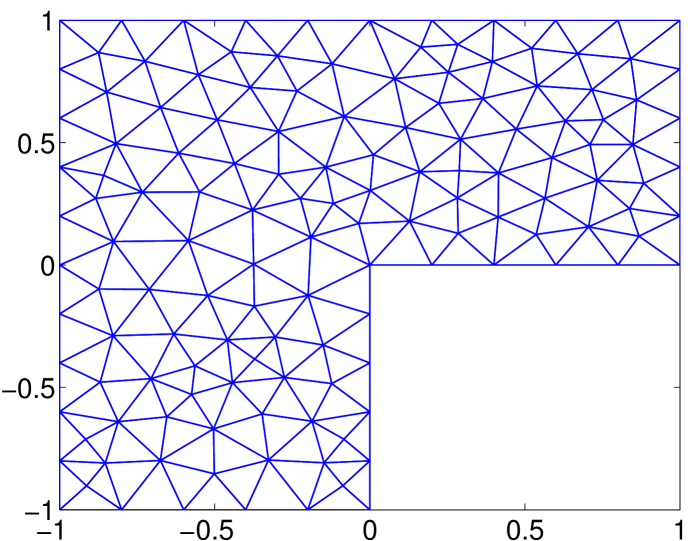
Fig. 1: Initial mesh of Example 3

The initial mesh is shown in Figure 1. The next level of mesh is derived by connecting middle point of each edge for the previous level of mesh. The error of numerical solution is shown in Table 5-6 for $k=2$ and $k=3.$ Here we can observe that ${|||}u_{h}-Q_{h}u{|||}$ approaches to zero at the rate $O(h^{2/3})$ as $h\to 0.$ However, the convergence rate of error in $L^{2}-norm$ is observed as $O(h^{1.4})$.

References

[1]D. N. Arnold and F. Brezzi, Mixed and nonconforming
finite element methods: implementation, postprocessing and error
estimates, RAIRO Mod l. Math. Anal. Num r., 19 (1985), 7-32.
[2]S, Brenner and L. Sung,
interior penalty methods for fourth order elliptic boundary value problems
on polygonal domains, J. Sci. Comput., 22 (2005), 83-118.
[3]G. Engel, K. Garikipati, T. Hughes, M.G. Larson, L. Mazzei, and R. Taylor, Con-
tinuous/discontinuous finite element approximations of fourth order elliptic problems in
structural and continuum mechanics with applications to thin beams and plates, and strain
gradient elasticity, Comput. Meth. Appl. Mech. Eng., 191 (2002), 3669-3750.
[4]R. FalkApproximation of the biharmonic equation by a mixed finite element method, SIAM J. Numer.
Anal., 15 (1978), 556-567.
[5]T. Gudi, N. Nataraj, A. K. Pani,
Mixed Discontinuous Galerkin Finite Element Method
for the Biharmonic Equation, J Sci Comput, 37 (2008), 139-161.
[6]A. Khamayseh1 and V. Almeida, Adaptive Hybrid Mesh Refinement for Multiphysics Applications,
Journal of Physics: Conference Series, 78 (2007) 12-39.
[7]L.S.D. Morley, The triangular equilibrium element in the solution of plate bending problems,
Aero. Quart., 19 (1968), 149-169.
[8]P. Monk, A mixed finite element methods for the biharmonic equation, SIAM J. Numer. Anal., 24 (1987), 737-749.
[9]I. Mozolevski and E. S li, B sing, P.R.: hp-Version a priori error analysis of interior penalty discontinuous
Galerkin finite element approximations to the biharmonic equation, J. Sci. Comput. 30 (2007), 46-71.
[10]L. Mu, Y. Wang, J. Wang and X. Ye,Weak Galerkin mixed finite element method for the biharmonic equation, Numerical Solution of Partial Differential Equations: Theory, Algorithms, and Their Applications, 45 (2013), 247-277.
[11]L. Mu, J. Wang, and X. Ye, A weak Galerkin finite element method for biharmonic equations on polytopal meshes, Numer. Meth. PDE, 30 (2014), 1003-1029.
[12]C. Wang and J. Wang, A hybridized weak Galerkin finite element method for the biharmonic equation, Int. J. Numer. Anal. Mod., 12 (2015), 302-317.
[13]J. Wang and X. Ye, A weak Galerkin finite element method
for second-order elliptic problems, J. Comp. and Appl. Math, 241 (2013), 103-115.
[14]J. Wang and X. Ye, A Weak Galerkin mixed finite element method for second-order elliptic problems, Math. Comp., 83 (2014),2101-2126.
[15]Q. Zhai, R. Zhang, and X. Wang, A hybridized weak Galerkin finite element scheme for the Stokes equations, Science China Mathematics, 58 (2015), 2455-2472.
[16]R. Zhang and Q. Zhai, A New Weak Galerkin Finite Element Scheme for Biharmonic Equations by Using Polynomials of Reduced Order, J. Sci. Comput., 64 (2015), 559-585.