Compressing Graphs and Indexes with Recursive Graph Bisection

Abstract

Graph reordering is a powerful technique to increase the locality of the representations of graphs, which can be helpful in several applications. We study how the technique can be used to improve compression of graphs and inverted indexes.

We extend the recent theoretical model of Chierichetti et al. (KDD 2009) for graph compression, and show how it can be employed for compression-friendly reordering of social networks and web graphs and for assigning document identifiers in inverted indexes. We design and implement a novel theoretically sound reordering algorithm that is based on recursive graph bisection.

Our experiments show a significant improvement of the compression rate of graph and indexes over existing heuristics. The new method is relatively simple and allows efficient parallel and distributed implementations, which is demonstrated on graphs with billions of vertices and hundreds of billions of edges.

1 Introduction

Many real-world systems and applications use in-memory representation of indexes for serving adjacency information in a graph. A popular example is social networks in which the list of friends is stored for every user. Another example is an inverted index for a collection of documents that stores, for every term, the list of documents where the term occurs. Maintaining these indexes requires a compact, yet efficient, representation of graphs.

How to represent and compress such information? Many techniques for graph and index compression have been studied in the literature [37, 24]. Most techniques first sort vertex identifiers in an adjacency list, and then replace the identifiers (except the first) with differences between consecutive ones. The resulting gaps are encoded using some integer compression algorithm. Note that using gaps instead of original identifiers decreases the values needed to be compressed and results in a higher compression ratio. We stress that the success of applying a particular encoding algorithm strongly depends on the distribution of gaps in an adjacency list: a sequence of small and regular gaps is more compressible than a sequence of large and random ones.

This observation has motivated the approach of assigning identifiers in a way that optimizes compression. Graph reordering has been successfully applied for social networks [13, 8]. In that scenario, placing similar social actors nearby in the resulting order yields a significant compression improvement. Similarly, lexicographic locality is utilized for compressing the Web graph: when pages are ordered by URL, proximal pages have similar sets of neighbors, which results in an increased compression ratio of the graph, when compared with the compression obtained using the original graph [29, 9]. In the context of index compression, the corresponding approach is called the document identifier assignment problem. Prior work shows that for many collections, index compression can be significantly improved by assigning close identifiers to similar documents [32, 34, 15, 6, 7].

In this paper, we study the problem of finding the best “compression-friendly” order for a graph or an inverted index. While graph reordering and document identifier assignment are often studied independently, we propose a unified model that generalizes both of the problems. Although a number of heuristics for the problems exists, none of them provides any guarantees on the resulting quality. In contrast, our algorithm is inspired by a theoretical approach with provable guarantees on the final quality, and it is designed to directly optimize the resulting compression ratio. Our main contributions are the following.

• We analyze and extend the formal model of graph compression suggested in [13]; the new model is suitable for both graph reordering and document identifier assignment problems. We show that the underlying optimization problem is NP-hard (thus, resolving an open question stated in [13]), and suggest an efficient approach for solving the problem, which is based on approximation algorithms for graph reordering.

• Based on the theoretical result, we develop a practical algorithm for constructing compression-friendly vertex orders. The algorithm uses recursive graph bisection as a subroutine and tries to optimize a desired objective at every recursion step. Our objective corresponds to the size of the graph compressed using delta-encoding. The algorithm is surprisingly simple, which allows for efficient parallel and distributed implementations.

• Finally, we perform an extensive set of experiments on a collection of large real-world graphs, including social networks, web graphs, and search indexes. The experiments indicate that our new method outperforms the state-of-the-art graph reordering techniques, improving the resulting compression ratio. Our implementation is highly scalable and is able to process a billion-vertex graph in a few hours.

The paper is organized as follows. We first discuss existing approaches for graph reordering, assigning document identifiers, and the most popular encoding schemes for graph and index representation (Section 2). Then we consider algorithmic aspects of the underlying optimization problem. We analyze the models for graph compression suggested by Chierichetti et al. [13] and suggest our generalization in Section 3.1. Next, in Section 3.2, we examine existing theoretical techniques for the graph reordering problem and use the ideas to design a practical algorithm. A detailed description of the algorithm along with the implementation details is presented in Section 4, which is followed by experimental Section 5. We conclude the paper with the most promising future directions in Section 6.

2 Related Work

There exists a rich literature on graph and index compression, that can be roughly divided into three categories: (1) structural approaches that find and merge repeating graph patterns (e.g., cliques), (2) encoding adjacency data represented by a list of integers given some vertex/document order, and (3) finding a suitable order of graph vertices. Our focus is on the ordering techniques. We discuss the existing approaches for graph reordering, followed by an overview of techniques for document identifier assignment. Since many integer encoding algorithms can benefit from such a reordering, we also outline the most popular encoding schemes.

Graph Reordering

Among the first approaches for compressing large-scale graphs is a work by Boldi and Vigna [9], who compress web graphs using a lexicographical order of the URLs. Their compression method relies on two properties: locality (most links lead to pages within the same host) and similarity (pages on the same host often share the same links). Later Apostolico and Drovandi [2] suggest one of the first ways to compress a graph assuming no a priori knowledge of the graph. The technique is based on a breadth-first traversal of the graph vertices and achieves a better compression rate using an entropy-based encoding.

Chierichetti et al. [13] consider the theoretical aspect of the reordering problem motivated by compressing social networks. They develop a simple but practical heuristic for the problem, called shingle ordering. The heuristic is based on obtaining a fingerprint of the neighbors of a vertex and positioning vertices with identical fingerprints close to each other. If the fingerprint can capture locality and similarity of the vertices, then it can be effective for compression. This approach is also called minwise hashing and was originally applied by Broder [10] for finding duplicate web pages.

Boldi et al. [8] suggest a reordering algorithm, called Layered Label Propagation, to compress social networks. The algorithm is built on a scalable graph clustering technique by label propagation [28]. The idea is to assign a label for every vertex of a graph based on the labels of its neighbors. The process is executed in rounds until no more updates take place. Since the standard label propagation described in [28] tends to produce a giant cluster, the authors of [8] construct a hierarchy of clusters. The vertices of the same cluster are then placed together in the final order.

The three-step multiscale paradigm is often employed for the graph ordering problems. First, a sequence of coarsened graphs, each approximating the original graph but having a smaller size, is created. Then the problem is solved on the coarsest level by an exhaustive search. Finally, the process is reverted by an uncoarsening procedure so that a solution for every graph in the sequence is based on the solution for a previous smaller graph. Safro and Temkin [31] employ the algebraic multigrid methodology in which the sequence of coarsened graphs is constructed using a projection of graph Laplacians into a lower-dimensional space.

Spectral methods have also been successfully applied to graph ordering problems [20]. Sequencing the vertices is done by sorting them according to corresponding elements of the second smallest eigenvector of graph Laplacian (also called the Fiedler vector). It is known that the order yields the best non-trivial solution to a relaxation of the quadratic graph ordering problem, and hence, it is a good heuristic for computing linear arrangements.

Recently Kang and Faloutsos [23] present another technique, called SlashBurn. Their method constructs a permutation of graph vertices so that its adjacency matrix is comprised of a few nonzero blocks. Such dense blocks are easier to encode, which is beneficial for compression.

In our experiments, we compare our new algorithm with all of the methods, which are either easy to implement, or come with the source code provided by the authors.

Document Identifier Assignment

Several papers study how to assign document identifiers in a document collection for better compression of an inverted index. A popular idea is to perform a clustering on the collection and assign close identifiers to similar documents. Shieh et al. [32] propose a reassignment heuristic motivated by the maximum travelling salesman problem (TSP). The heuristic computes a pairwise similarity between every pairs of documents (proportional to the number of shared terms), and then finds the longest path traversing the documents in the graph. An alternative algorithm calculating cosine similarities between documents is suggested by Blandford and Blelloch [7]. Both methods are computationally expensive and are limited to fairly small datasets. The similarity-based approach is later improved by Blanco and Barreiro [6] and by Ding et al. [15], who make it scalable by reducing the size of the similarity graph, respectively through dimensionality reduction and locality sensitive hashing.

The approach by Silvestri [34] simply sorts the collection of web pages by their URLs and then assigns document identifiers according to the order. The method performs very well in practice and is highly scalable. This technique however does not generalize to document collections that do not have URL-like identifiers.

Encoding Schemes

Our algorithm is not tailored specifically for an encoding scheme; any method that can take advantage of lists with higher local density (clustering) should benefit from the reordering. For our experiment we choose a few encoding schemes that should be representative of the state-of-the-art.

Most graph compression schemes build on delta-encoding, that is, sorting the adjacency lists (posting lists in the inverted indexes case) so that the gaps between consecutive elements are positive, and then encoding these gaps using a variable-length integer code. The WebGraph framework adds the ability to copy portions of the adjacency lists from other vertices, and has special cases for runs of consecutive integers. Introduced in 2004 by Boldi and Vigna [9], it is still widely used to compress web graphs and social networks.

Inverted indexes are usually compressed with more specialized techniques in order to enable fast skipping, which enables efficient list intersection. We perform our experiments with Partitioned Elias-Fano and Binary Interpolative Coding. The former, introduced by Ottaviano and Venturini [26], provides one of the best compromise between decoding speed and compression ratio. The latter, introduced by Moffat and Stuiver [25], has the highest compression ratio in the literature, with the trade-off of slower decoding by several times. Both techniques directly encode monotone lists, without going through delta-encoding.

3 Algorithmic Aspects

Graph reordering is a combinatorial optimization problem with a goal to find a linear layout of an input graph so that a certain objective function (referred to as a cost function or just cost) is optimized. A linear layout of a graph $G=(V,E)$ with $n=|V|$ vertices is a bijection $\pi:V\rightarrow\{1,\dots,n\}$. A layout is also called an order, an arrangement, or a numbering of the vertices. In practice it is desirable that “similar” vertices of the graph are “close” in $\pi$. This leads to a number of problems that we define next.

The minimum linear arrangement (MLA) problem is to find a layout $\pi$ so that

$$\sum_{(u,v)\in E}|\pi(u)-\pi(v)|$$

is minimized. This is a classical NP-hard problem [18], even when restricted to certain graph classes. The problem is APX-hard under Unique Games Conjecture [14], that is, it is unlikely that an efficient approximation algorithm exists. Charikar et al. [11] suggested the best currently known algorithm with approximation factor ${\mathcal{O}}(\sqrt{\log n}\log\log n)$; see [27] for a survey of results on MLA.

A closely related problem is minimum logarithmic arrangement (MLogA) in which the goal is to minimize

$$\sum_{(u,v)\in E}\log|\pi(u)-\pi(v)|.$$

Here and in the following we denote $\log(x)=1+\lfloor\log_{2}(x)\rfloor$, that is, the number of bits needed to represent an integer $x$. The problem is also NP-hard, and one can show that the optimal solutions of MLA and MLogA are quite different on some graphs [13]. In practice a graph is represented in memory as an adjacency list using an encoding scheme; hence, the gaps induced by consecutive neighbors of a vertex are important for compression. For this reason, the minimum logarithmic gap arrangement (MLogGapA) problem is introduced. For a vertex $v\in V$ of degree $k$ and an order $\pi$, consider the neighbors $out(v)=(v_{1},\dots,v_{k})$ of $v$ such that $\pi(v_{1})<\dots<\pi(v_{k})$. Then the cost compressing the list $out(v)$ under $\pi$ is related to $f_{\pi}(v,out(v))=\sum_{i=1}^{k-1}\log|\pi(v_{i+1})-\pi(v_{i})|$. MLogGapA consists in finding an order $\pi$, which minimizes

$$\sum_{v\in V}f_{\pi}(v,out(v)).$$

To the best of our knowledge, MLogA and MLogGapA are introduced quite recently by Chierichetti et al. [13]. They show that MLogA is NP-hard but left the computational complexity of MLogGapA open. Since the latter problem is arguably more important for applications, we address the open question of complexity of the problem.

Theorem 1.

MLogGapA is NP-hard.

Proof.

We prove the theorem by using the hardness of MLogA, which is known to be NP-hard [13]. Let $G=(V,E)$ be an instance of MLogA. We build a bipartite graph $G^{\prime}=(V^{\prime},E^{\prime})$ by splitting every edge of $E$ by a degree-2 vertex. Formally, we add $|E|$ new vertices so that $V^{\prime}=V\cup U$, where $V=\{v_{1},\dots,v_{n}\}$ and $U=\{u_{1},\dots,u_{m}\}$. For every edge $(a,b)\in E$, we have two edges in $E^{\prime}$, that is, $(a,u_{i})$ and $(b,u_{i})$ for some $1\leq i\leq m$. Next we show that an optimal solution for MLogGapA on $G^{\prime}$ yields an optimal solution for MLogA on $G$, which proves the claim of the theorem.

Let $R$ be an optimal order of $V^{\prime}$ for MLogGapA. Observe that without loss of generality, the vertices of $V$ and $U$ are separated in $R$, that is, $R=(v_{i_{1}},\dots,v_{i_{n}},u_{j_{1}},\dots,u_{j_{m}})$. Otherwise, the vertices can be reordered so that the total objective is not increased. To this end, we “move” all the vertices of $V$ to the left of $R$ by preserving their relative order. It is easy to see that the gaps between vertices of $V$ and the gaps between vertices of $U$ can only decrease.

Now the cost of MLogGapA is

$$\sum_{v\in V}f_{\pi_{u}}(v,out(v))+\sum_{u\in U}f_{\pi_{v}}(u,out(u)),$$

where $\pi_{u}=(u_{j_{1}},\dots,u_{j_{m}})$ and $\pi_{v}=(v_{i_{1}},\dots,v_{i_{n}})$. Notice that the second term of the sum depends only on the order $\pi_{v}$ of the vertices in $V$, and it equals to the cost of MLogA for graph $G$. Since $R$ is optimal for MLogGapA, the order $\pi_{v}=(v_{i_{1}},\dots,v_{i_{n}})$ is also optimal for MLogA. ∎

Most of the previous works consider the MLogA problem for graph compression, and the algorithms are not directly suitable for index compression. Contrarily, an inverted index is generally represented by a directed graph (with edges from terms to documents), which is not captured by the MLogGapA problem. In the following, we suggest a model, which generalizes both MLogA and MLogGapA and better expresses graph and index compression.

3.1 Model for Graph and Index Compression

Intuitively, our new model is a bipartite graph comprising of query and data vertices. A query vertex might correspond to an actor in a social network or to a term in an inverted index. Data vertices are an actor’s friends or documents containing the term, respectively. The goal is to find a layout of data vertices.

Formally, let $G=(\mathcal{Q}\cup\mathcal{D},E)$ be an undirected unweighted bipartite graph with disjoint sets of vertices $\mathcal{Q}$ and $\mathcal{D}$. We denote $|\mathcal{D}|=n$ and $|E|=m$. The goal is to find a permutation, $\pi$, of data vertices, $\mathcal{D}$, so that the following objective is minimized:

$$\sum_{q\in\mathcal{Q}}\sum_{i=1}^{\deg_{q}-1}\log(\pi(u_{i+1})-\pi(u_{i})),$$

where $\deg_{q}$ is the degree of query vertex $q\in\mathcal{Q}$, and $q$’s neighbors are $\{u_{1},\dots,u_{deg_{q}}\}$ with $\pi(u_{1})<\dots<\pi(u_{deg_{q}})$. Note that the objective is closely related to minimizing the number of bits needed to store a graph or an index represented using the delta-encoding scheme. We call the optimization problem bipartite minimum logarithmic arrangement (BiMLogA), and the corresponding cost averaged over the number of gaps $\operatorname{LogGap}$.

Note that BiMLogA is different from MLogGapA in that the latter does not differentiate between data and query vertices (that is, every vertex is query and data in MLogGapA), which is unrealistic in some applications. It is easy to see that the new problem generalizes both MLogA and MLogGapA: to model MLogA, we add a query vertex for every edge of the input graph, as in the proof of Theorem 1; to model MLogGapA, we add a query for every vertex of the input graph; see Figure 1. Moreover, the new approach can be naturally applied for compressing directed graphs; to this end, we only consider gaps induced by outgoing edges of a vertex. Clearly, given an algorithm for BiMLogA, we can easily solve both MLogA and MLogGapA. Therefore, we focus on this new problem in the next sections.

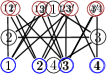
(a) Original graph

(b) MLogA

(c) MLogGapA

Figure 1: Modeling of MLogA and MLogGapA with a bipartite graph with query (red) and data (blue) vertices.

How can one solve the above ordering problems? Next we discuss the existing theoretical approaches for solving graph ordering problems. We focus on approximation algorithms, that is, efficient algorithms for NP-hard problems that produce sub-optimal solutions with provable quality.

3.2 Approximation Algorithms

To the best of our knowledge, no approximation algorithms exist for the new variants of the graph ordering problem. However, a simple observation shows that every algorithm has approximation factor ${\mathcal{O}}(\log n)$. Note that the cost of a gap between $u\in\mathcal{D}$ and $v\in\mathcal{D}$ in BiMLogA cannot exceed $\log n$, as $|\pi(v)-\pi(u)|\leq n$ for every permutation $\pi$. On the other hand, the cost of a gap is at least $1$. Therefore, an arbitrary order of vertices yields a solution with the cost, which is at most $\log n$ times greater than the optimum.

In contrast, the well-studied MLA does not admit such a simple approximation and requires more involved algorithms. We observe that most of the existing algorithms for MLA and related ordering problems employ the divide-and-conquer approach; see Algorithm 1. Such algorithms partition the vertex set into two sets of roughly equal size, compute recursively an order of each part, and “glue” the orderings of the parts together. The crucial part is graph bisection or more generally balanced graph partitioning, if the graph is split into more than two parts.

Input : graph $G$

1. Find a bisection $(G_{1},G_{2})$ of $G$;

2. Recursively find linear arrangements for $G_{1}$ and $G_{2}$;

3. Concatenate the resulting orderings;

Algorithm 1 Graph Reordering using Graph Bisection

The first non-trivial approximation algorithm for MLA follows the above approach. Hancen [19] proves that Algorithm 1 yields an ${\mathcal{O}}(\alpha\log n)$-approximation for MLA, where $\alpha$ indicates how close is the solution of the first step (bisection of $G$) to the optimum. Later, Charikar et al. [12] shows that a tighter analysis is possible, and the algorithm is in fact ${\mathcal{O}}(\alpha)$-approximation for $d$-dimensional MLA. Currently, $\alpha={\mathcal{O}}(\sqrt{\log n})$ is the best known bound [3]. Subsequently, the idea of Algorithm 1 was employed by Even et al. [16], Rao and Richa [30], and Charikar et al. [11] for composing approximation algorithms for MLA. The techniques use the recursive divide-and-conquer approach and utilize a spreading metric by solving a linear program with an exponential number of constraints.

Inspired by the algorithms, we design a practical approach for the BiMLogA problem. While solving a linear program is not feasible for large graphs, we utilize recursive graph partitioning in designing the algorithm. Next we describe all the steps and provide implementation-specific details.

4 Compression-Friendly Graph Reordering

Assume that the input is an undirected bipartite graph $G=(\mathcal{Q}\cup\mathcal{D},E)$, and the goal is to compute an order of $\mathcal{D}$. On a high level, our algorithm is quite simple; see Algorithm 1.

The reordering method is based on the graph bisection problem, which asks for a partition of graph vertices into two sets of equal cardinality so as to minimize an objective function. Given an input graph $G$ with $|\mathcal{D}|=n$, we apply the bisection algorithm to obtain two disjoint sets $V_{1},V_{2}\subseteq\mathcal{D}$ with $|V_{1}|=\lfloor n/2\rfloor$ and $|V_{2}|=\lceil n/2\rceil$. We shall lay out $V_{1}$ on the set $\{1,\dots,\lfloor n/2\rfloor\}$ and lay out $V_{2}$ on the set $\{\lceil n/2\rceil,\dots,n\}$. Thus, we have divided the problem into two problems of half the size, and we recursively compute good layouts for the graphs induced by $V_{1}$ and $V_{2}$, which we call $G_{1}$ and $G_{2}$, respectively. Of course, when there is only one vertex in $G$, the order is trivial.

How to bisect the vertices of the graph? We use a graph bisection method, similar to the popular Kernighan-Lin heuristic [21]; see Algorithm 2. Initially we split $\mathcal{D}$ into two sets, $V_{1}$ and $V_{2}$, and define a computational cost of the partition, which indicates how “compression-friendly” the partition is. Next we exchange pairs of vertices in $V_{1}$ and $V_{2}$ trying to improve the cost. To this end we compute, for every vertex $v\in\mathcal{D}$, the move gain, that is, the difference of the cost after moving $v$ from its current set to another one. Then the vertices of $V_{1}$ ($V_{2}$) are sorted in the decreasing order of the gains to produce list $S_{1}$ ($S_{2}$). Finally, we traverse the lists $S_{1}$ and $S_{2}$ in the order and exchange the pairs of vertices, if the sum of their move gains is positive. Note that unlike classical graph bisection heuristics [21, 17], we do not update move gains after every swap. The process is repeated until the convergence criterion is met (no swapped vertices) or the maximum number of iterations is reached.

Input : graph $G=(\mathcal{Q}\cup\mathcal{D},E)$

Output : graphs $G_{1}=(\mathcal{Q}\cup V_{1},E_{1}),G_{2}=(\mathcal{Q}\cup V_{2},E_{2})$

determine an initial partition of $\mathcal{D}$ into $V_{1}$ and $V_{2}$;

repeat

       for $v\in\mathcal{D}$ do

            $gains[v]\leftarrow ComputeMoveGain(v)$

      $S_{1}\leftarrow$ sorted $V_{1}$ in descending order of $gains$;

       $S_{2}\leftarrow$ sorted $V_{2}$ in descending order of $gains$;

       for $v\in S_{1}$, $u\in S_{2}$ do

             if $gains[v]+gains[u]>0$ then

                   exchange $v$ and $u$ in the sets;

            else break;

            

      

until converged or iteration limit exceeded;

return graphs induced by $\mathcal{Q}\cup V_{1}$ and $\mathcal{Q}\cup V_{2}$

Algorithm 2 Graph Bisection

To initialize the bisection, we consider the following two alternatives. A simpler one is to arbitrarily split $\mathcal{D}$ into two equal-sized sets. Another approach is based on shingle ordering (minwise hashing) suggested in [13]. To this end, we order the vertices as described in [13] and assign the first $\lfloor n/2\rfloor$ vertices to $V_{1}$ and the last $\lceil n/2\rceil$ to $V_{2}$.

Algorithm 2 tries to minimize the following objective function of the sets $V_{1}$ and $V_{2}$, which is motivated by BiMLogA. For every vertex $q\in\mathcal{Q}$, let $\deg_{1}(q)=|\{(q,v):v\in V_{1}\}|$, that is, the number of adjacent vertices in set $V_{1}$; define $\deg_{2}(q)$ similarly. Then the cost of the partition is

$$\sum_{q\in\mathcal{Q}}\left(\deg_{1}(q)\log(\frac{n_{1}}{\deg_{1}(q)+1})+\deg_{2}(q)\log(\frac{n_{2}}{\deg_{2}(q)+1})\right),$$

where $n_{1}=|V_{1}|$ and $n_{2}=|V_{2}|$. The cost estimates the required number of bits needed to represent $G$ using delta-encoding. If the neighbors of $q\in\mathcal{Q}$ are uniformly distributed in the final arrangement of $V_{1}$ and $V_{2}$, then the the average gap between consecutive numbers in the $q$’s adjacency list is $\operatorname{gap}_{1}\coloneqq n_{1}/(\deg_{1}(q)+1)$ and $\operatorname{gap}_{2}\coloneqq n_{2}/(\deg_{2}(q)+1)$ for $V_{1}$ and $V_{2}$, respectively; see Figure 2. There are $(\deg_{1}(q)-1)$ gaps between vertices in $V_{1}$ and $(\deg_{2}(q)-1)$ gaps between vertices in $V_{2}$. Hence, we need approximately $(\deg_{1}(q)-1)\log(\operatorname{gap}_{1})+(\deg_{2}(q)-1)\log(\operatorname{gap}_{2})$ bits to compress the within-group gaps. In addition, we have to account for the average gap between the last vertex of $V_{1}$ and the first vertex of $V_{2}$, which is $(\operatorname{gap}_{1}+\operatorname{gap}_{2})$. Assuming that $n_{1}=n_{2}$, we have $\log(\operatorname{gap}_{1}+\operatorname{gap}_{2})=\log(\operatorname{gap}_{1})+\log(\operatorname{gap}_{2})+C$, where $C$ is a constant with respect to the data vertex assignment, and hence, it can be ignored in the optimization. Adding this between-group contribution to the within-group contributions gives the above expression.

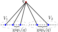
Figure 2: Partitioning $\mathcal{D}$ into $V_{1}$ and $V_{2}$ for a query $q\in\mathcal{Q}$ with $\deg_{1}(q)=3$ and $\deg_{2}(q)=2$.

Note that using the cost function, it is straightforward to implement $ComputeMoveGain(v)$ function from Algorithm 2 by traversing all the edges $(q,v)\in E$ for $v\in\mathcal{D}$ and summing up the cost differences of moving $v$ to another set.

Combining all the steps of Algorithm 1 and Algorithm 2, we have the following claim.

Theorem 2.

The algorithm produces a vertex order in ${\mathcal{O}}(m\log n+n\log^{2}n)$ time.

Proof.

There are $\lceil\log n\rceil$ levels of recursion. Each call of graph bisection requires computing move gains and sorting of $n$ elements. The former can be done in ${\mathcal{O}}(m)$ steps, while the latter requires ${\mathcal{O}}(n\log n)$ steps. Summing over all subproblems, we get the claim of the theorem. ∎

4.1 Implementation

Due to the simplicity of the algorithm, it can be efficiently implemented in parallel or distributed manner. For the former, we notice that two different recursive calls of Algorithm 1 are independent, and thus, can be executed in parallel. Analogously, a single bisection procedure can easily be parallelized, as each of its steps computes independent values for every vertex, and a parallel implementation of sorting can be used. In our implementation, we employ the fork-join computation model in which small enough graphs are processed sequentially, while larger graphs which occur on the first few levels of recursion are solved in parallel manner.

Our distributed implementation relies on the vertex-centric programming model and runs in the Giraph framework. In Giraph, a computation is split into supersteps that consists of processing steps: (i) a vertex executes a user-defined function based on local vertex data and on data from adjacent vertices, (ii) the resulting output is sent along outgoing edges. Supersteps end with a synchronization barrier, which guarantees that messages sent in a given superstep are received at the beginning of the next superstep. The whole computation is executed iteratively for a certain number of rounds, or until a convergence property is met.

Algorithm 2 is implemented in the vertex-centric model with a simple modification. The first two supersteps compute move gains for all data vertices. To this end, every query vertex calculates the differences of the cost function when its neighbor moves from a set to another one. Then, every data vertex sums up the differences over its query neighbors. Given the move gains, we exchange the vertices as follows. Instead of sorting the move gains, we construct, for both sets, an approximate histogram (e.g., as described in [5]) of the gain values. Since the size of the histograms is small enough, we collect the data on a dedicated host, and decide how many vertices from each bin should exchange its set. On the last superstep, this information is propagated over all data vertices and the corresponding swaps take effect.

5 Experiments

We design our experiments to answer two primary questions: (i) How well does our algorithm compress graphs and indexes in comparison with existing techniques? (ii) How do various parameters of the algorithm contribute to the solution, and what are the best parameters?

5.1 Dataset

For our experiments, we use several publicly available web graphs, social networks, and inverted document indexes; see Table 1. In addition, we run evaluation on two large subgraphs of the Facebook friendship graph and a sample of the Facebook search index. These private datasets serve to demonstrate scalability of our approach. We do not release the datasets and our source code due to corporate restrictions. Before running the tests, all the graphs are made unweighted and converted to bipartite graphs as described in Section 3.1. Our dataset is as follows.

• Enron represents an email communication network; data is available at https://snap.stanford.edu/data.

• AS-Oregon is an Autonomous Systems peering information inferred from Oregon route-views in 2001; data is available at https://snap.stanford.edu/data.

• FB-NewOrlean contains a list of all of the user-to-user links from the Facebook New Orleans network; the data was crawled and anonymized in 2009 [36].

• web-Google represents web pages with hyperlinks between them. The data was released in 2002 by Google; data is available at https://snap.stanford.edu/data.

• LiveJournal is an undirected version of the public social graph (snapshot from 2006) containing $4.8$ million vertices and $42.9$ million edges [35].

• Twitter is a public graph of tweets, with about $41$ million vertices (twitter accounts) and $2.4$ billion edges (denoting followership) [22].

• Gov2 is an inverted index built on the TREC 2004 Terabyte Track test collection, consisting of 25 million .gov sites crawled in early 2004.

• ClueWeb09 is an inverted index built on the ClueWeb 2009 TREC Category B test collection, consisting of 50 million English web pages crawled in 2009.

• FB-Posts-1B is an inverted index built on a sample of one billion Facebook posts, containing the longest posting lists. Since the posts have no hierarchical URLs, the Natural order for this index is random.

• FB-300M and FB-1B are two subgraphs of the Facebook friendship graph; the data was anonymized before processing.

To build the inverted indexes for Gov2 and ClueWeb09 the body text was extracted using Apache Tika and the words were lowercased and stemmed using the Porter2 stemmer; no stopwords were removed. We consider only long posting lists containing more than $4096$ elements.

Graph	$|\mathcal{Q}|$	$|\mathcal{D}|$	$|E|$
Enron	$9,\!660$	$9,\!660$	$224,\!896$
AS-Oregon	$13,\!579$	$13,\!579$	$74,\!896$
FB-NewOrlean	$63,\!392$	$63,\!392$	$1,\!633,\!662$
web-Google	$356,\!648$	$356,\!648$	$5,\!186,\!648$
LiveJournal	$4,\!847,\!571$	$4,\!847,\!571$	$85,\!702,\!474$
Twitter	$41,\!652,\!230$	$41,\!652,\!230$	$2,\!405,\!026,\!092$
Gov2	$39,\!187$	$24,\!618,\!755$	$5,\!322,\!924,\!226$
ClueWeb09	$96,\!741$	$50,\!130,\!884$	$14,\!858,\!911,\!083$
FB-Posts-1B	$60\times 10^{3}$	$1\times 10^{9}$	$20\times 10^{9}$
FB-300M	$300\times 10^{6}$	$300\times 10^{6}$	$90\times 10^{9}$
FB-1B	$1\times 10^{9}$	$1\times 10^{9}$	$300\times 10^{9}$

Table 1: Basic properties of our dataset.

5.2 Techniques

We compare our new algorithm (referred to as BP) with the following competitors.

• Natural is the most basic order defined for a graph. For web graphs and document indexes, the order is the URL lexicographic ordering used in [29, 9]. For social networks, the order is induced by the original adjacency matrix.

• BFS is given by the bread-first search graph traversal algorithm as utilized in [2].

• Minhash is the lexicographic order of $10$ minwise hashes of the adjacency sets. The same approach with only $2$ hashes is called double shingle in [13].

• TSP is a heuristic for document reordering suggested by Shieh et al. [32], which is based on solving the maximum travelling salesman problem. We implemented the variant of the algorithm that performs best in the authors’ experiments. Since the algorithm is computationally expensive, we run it on small instances only. The sparsification techniques presented in [6, 15] would allow us to scale to the larger graphs, but they are too complex to re-implement faithfully.

• LLP represents an order computed by the Layered Label Propagation algorithm [8].

• Spectral order is given by the second smallest eigenvector of the Laplacian matrix of the graph [20].

• Multiscale is an algorithm based on the multi-level algebraic methodology suggested for solving MLogA [31].

• SlashBurn is a method for matrix reordering [23].

5.3 Effect of BP parameters

BP has a number of parameters that can affect its quality and performance. In the following we discuss some of the parameters and explain our choice of their default values.

An important aspect of BP is how two sets, $V_{1}$ and $V_{2}$, are initialized in Algorithm 2. Arguably the initialization procedure might affect the quality of the final vertex order. To verify the hypothesis, we implemented four initialization techniques that bisect a given graph: Random, Natural, BFS, and Minhash. The techniques order the data vertices, $\mathcal{D}$, using the corresponding algorithm, and then split the order into two sets of equal size. In the experiment, we intentionally consider only the simplest and most efficient bisection techniques so as to keep the complexity of the BP algorithm low. Figure 4 illustrates the effect of the initialization methods for graph bisection. Note that initialization plays a role to some extent, and there is no consistent winner. BFS is the best initialization for three of the graphs but does not produce an improvement on the indexes. One explanation is that the indexes contain high-degree query vertices, that make the BFS order essentially random. Overall, the difference between the final results is not substantial, and even the worst initialization yields better orders than the alternative algorithms do. Therefore, we utilize the simplest approach, Random, for graphs and Minhash for indexes as the default technique for bisection initialization.

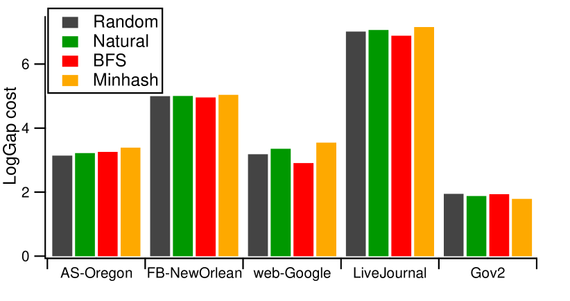
Figure 3: $\operatorname{LogGap}$ cost of the resulting order produced with different initialization approaches for graph bisection.

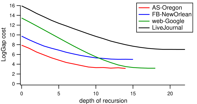
Figure 4: $\operatorname{LogGap}$ cost of the resulting order produced with a fixed depth of recursion. Note that the last few splits make insignificant contributions to the final quality.

Is it always necessary to perform $\log n$ levels of recursion to get a reasonable solution? Figure 4 shows the quality of the resulting vertex order after a fixed number, $i$, of recursion splits. For every $i$ (that is, when there are $2^{i}$ disjoint sets), we stop the algorithm and measure the quality of the order induced by the random assignment of vertices respecting the partition. It turns out that graph bisection is beneficial only when $\mathcal{D}$ contains more than a few tens of vertices. In our implementation, we set $(\log n-5)$ for the depth of recursion, which slightly reduces the overall running time. It might be possible to improve the final quality by finding an optimal solution (e.g., using an exhaustive search or a linear program) for small subgraphs on the lowest levels of the recursion. We leave the investigation for future research.

Figure 5 illustrates the speed of convergence of our optimization procedure utilized for improving graph partitioning in Algorithm 2. The two sets approach a locally optimal state within a few iterations. The number of required iterations increases, as the depth of recursion gets larger. Generally, the number of moved vertices per iteration does not exceed $1\%$ after $20$ iterations, even for the deepest recursion levels. Therefore, we use $20$ as the default number of iterations in all our experiments.

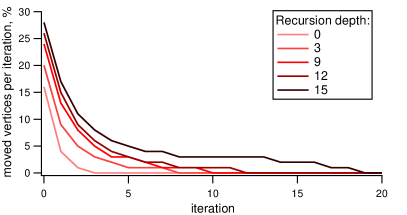
Figure 5: The average percentage of moved vertices on an iteration of Algorithm 2 for various levels of recursion. The data is computed for LiveJournal.

(a) Natural

(b) BFS

(c) Minhash

(d) TSP

(e) LLP

(f) Spectral

(g) Multiscale

(h) SlashBurn

(i) BP

Figure 6: Adjacency matrices of FB-NewOrlean after applying various reordering algorithms; nonzero elements are blue.

5.4 Compression ratio

Table 2 presents a comparison of various reordering methods on social networks and web graphs. We evaluate the following measures: (i) the cost of the BiMLogA problem ($\operatorname{LogGap}$), (ii) the cost of the MLogA problem (the logarithmic difference averaged over the edges, $\operatorname{Log}$), (iii) the average number of bits per edge needed to encode the graph with WebGraph [9] (referred to as BV). The results suggest that BP yields the best compression on all but one instance, providing an $5-20\%$ improvement over the best alternative. An average gain over a non-reordered solution reaches impressive $50\%$. The runner-up approaches, TSP, LLP, and Multiscale, also significantly outperform the natural order. However, their straightforward implementations are not scalable for large graphs (none of them is able to process Twitter within a few hours), while efficient implementations are arguably more complicated than BP.

The computed results for FB-300M and FB-1B demonstrate that the new reordering technique is beneficial for very large graphs, too. Unfortunately, we were not able to calculate the compression rate for the graphs, as WebGraph [9] does not provide distributed implementation. However, the experiment indicates that BP outperforms Natural by around $50\%$ and outperforms Minhash by around $30\%$.

Graph	Algorithm	$\operatorname{LogGap}$	$\operatorname{Log}$	BV
Enron	Natural	$5.01$	$9.82$	$7.80$
	BFS	$4.86$	$9.97$	$7.70$
	Minhash	$4.91$	$10.12$	$7.68$
	TSP	$3.95$	$9.46$	$6.58$
	LLP	$3.96$	$8.55$	$6.51$
	Spectral	$5.43$	$9.41$	$8.60$
	Multiscale	$4.23$	$\boldsymbol{8.00}$	$6.90$
	SlashBurn	$5.11$	$10.18$	$8.05$
	BP	$\boldsymbol{3.69}$	$8.26$	$\boldsymbol{6.24}$
AS-Oregon	Natural	$7.88$	$12.06$	$13.34$
	BFS	$4.71$	$11.06$	$7.97$
	Minhash	$4.47$	$11.17$	$7.56$
	TSP	$3.59$	$10.39$	$6.66$
	LLP	$4.42$	$8.32$	$7.47$
	Spectral	$5.64$	$9.53$	$8.76$
	Multiscale	$4.53$	$\boldsymbol{7.23}$	$7.31$
	SlashBurn	$4.50$	$10.66$	$8.74$
	BP	$\boldsymbol{3.15}$	$9.21$	$\boldsymbol{6.25}$
FB-NewOrlean	Natural	$9.74$	$14.29$	$14.64$
	BFS	$7.16$	$12.63$	$10.79$
	Minhash	$7.06$	$12.57$	$10.62$
	TSP	$5.62$	$11.61$	$8.96$
	LLP	$5.37$	$\boldsymbol{9.41}$	$8.54$
	Spectral	$7.64$	$11.49$	$11.79$
	Multiscale	$5.90$	$9.58$	$9.25$
	SlashBurn	$8.37$	$13.06$	$12.65$
	BP	$\boldsymbol{4.99}$	$9.45$	$\boldsymbol{8.16}$
web-Google	Natural	$13.39$	$16.74$	$20.08$
	BFS	$5.57$	$11.21$	$7.69$
	Minhash	$5.65$	$13.14$	$6.87$
	TSP	$3.28$	$7.99$	$4.77$
	LLP	$3.75$	$6.70$	$5.13$
	Spectral	$6.68$	$10.25$	$9.16$
	Multiscale	$\boldsymbol{2.72}$	$\boldsymbol{4.82}$	$\boldsymbol{4.10}$
	SlashBurn	$8.02$	$14.46$	$10.29$
	BP	$3.17$	$7.74$	$4.68$
LiveJournal	Natural	$10.43$	$17.44$	$14.61$
	BFS	$10.52$	$17.59$	$14.69$
	Minhash	$10.79$	$17.76$	$15.07$
	LLP	$7.46$	$\boldsymbol{12.25}$	$11.12$
	BP	$\boldsymbol{7.03}$	$12.79$	$\boldsymbol{10.73}$
Twitter	Natural	$15.23$	$23.65$	$21.56$
	BFS	$12.87$	$22.69$	$17.99$
	Minhash	$10.43$	$21.98$	$14.76$
	BP	$\boldsymbol{7.91}$	$\boldsymbol{20.50}$	$\boldsymbol{11.62}$
FB-300M	Natural	$17.65$	$25.34$
	Minhash	$13.06$	$24.9$
	BP	$\boldsymbol{8.39}$	$\boldsymbol{18.13}$
FB-1B	Natural	$19.63$	$27.22$
	Minhash	$14.60$	$26.89$
	BP	$\boldsymbol{8.66}$	$\boldsymbol{18.36}$

Table 2: Reordering results of various algorithms on graphs: the costs of MLogA, BiMLogA, and the number of bits per edge required by BV. The best results in every column are highlighted. We present the results that completed the computation within a few hours.

Index	Algorithm	$\operatorname{LogGap}$	PEF	BIC
Gov2	Natural	$2.12$	$3.12$	$2.52$
	BFS	$2.07$	$3.00$	$2.44$
	Minhash	$2.12$	$3.12$	$2.52$
	BP	$\boldsymbol{1.81}$	$\boldsymbol{2.44}$	$\boldsymbol{1.95}$
ClueWeb09	Natural	$2.91$	$4.99$	$4.05$
	BFS	$2.91$	$4.99$	$4.06$
	Minhash	$2.91$	$4.99$	$4.05$
	BP	$\boldsymbol{2.55}$	$\boldsymbol{4.34}$	$\boldsymbol{3.50}$
FB-Posts-1B	Natural	$8.03$	$10.19$	$9.95$
	Minhash	$3.41$	$4.96$	$4.24$
	BP	$\boldsymbol{2.95}$	$\boldsymbol{4.18}$	$\boldsymbol{3.61}$

Table 3: Reordering results of various algorithms on inverted indexes with highlighted best results.

The compression ratio of inverted indexes is illustrated in Table 3, where we evaluate the Partitioned Elias-Fano [26] encoding and Binary Interpolative Coding [25] (respectively PEF and BIC). Here the results are reported in average bits per edge. Again, our new algorithm largely outperforms existing approaches in terms of both $\operatorname{LogGap}$ cost and compression rate. BP has a large impact on the indexes, achieving a $22\%$ and a $15\%$ compression improvement over alternatives; these gains are almost identical for PEF and BIC.

An interesting question is why does the new algorithm perform best on most of the tested graphs. In Figure 7 we analyze the number of gaps between consecutive numbers of graph adjacency lists. It turns out that BP and LLP have quite similar gap distributions, having notably more shorter gaps than the alternative methods. Note that the number of edges that the BV encoding is able to copy is related to the number of consecutive integers in the adjacency lists; hence short gaps strongly influences its performance. At the same time, BP is slightly better at longer gaps, which is a reason why the new algorithm yields a higher compression ratio.

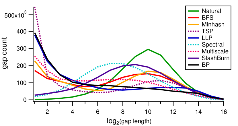
(a) FB-NewOrlean

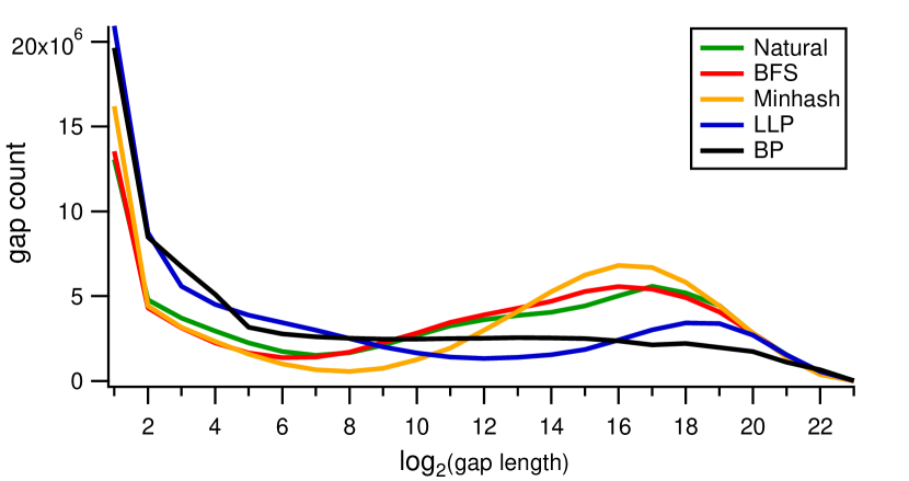
(b) LiveJournal

Figure 7: Distribution of gaps between consecutive elements of graph adjacency lists induced by various algorithms.

We point out that the cost of BiMLogA, $\operatorname{LogGap}$, is more relevant for the compression rate than the cost of MLogA; see Figure 8. The observation agrees with the previous evaluation of Boldi et al. [8] and motivates our research on the former problem. The Pearson correlation coefficients between the $\operatorname{LogGap}$ cost and the average number of bit per edge using BV, PEF, and BIC encoding schemes are $0.9853$, $0.8487$, and $0.8436$, respectively. While the high correlation between $\operatorname{LogGap}$ and BV is observed earlier [9, 13], the relation between $\operatorname{LogGap}$ and PEF or BIC is a new phenomenon. A possible explanation is that the schemes encode a sequence of $k$ integers in the range $[1..n]$ using close to the information-theoretic minimum of $k(1+\lfloor\log_{2}(n/k)\rfloor)$ bits [26], which is equivalent to our optimization function utilized in Algorithm 2. It might be possible to construct a better model for the two encoding schemes, where the cost of the optimization problem has a higher correlation with the final compression ratio. For example, this can be achieved by increasing the weights of “short” gaps that are generally require more than $\log(\operatorname{gap})$ bits. We leave the question for future investigation.

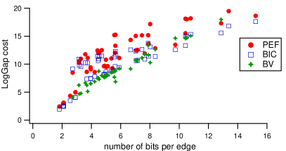
Figure 8: $\operatorname{LogGap}$ cost against the average number of bits per edge using various encoding schemes.

Figure 6 presents an alternative comparison of the impact of the reordering algorithms on the FB-NewOrlean graph. Note that only BP and LLP are able to find communities in the graph (dense subgraphs), that can be compressed efficiently. The recursive nature of BP is also clearly visible.

5.5 Running time

We created and tested two implementations of our algorithm, parallel and distributed. The parallel version is implemented in C++11 and compiled with the highest optimization settings. The tests are performed on a machine with Intel(R) Xeon(R) CPU E5-2660 @ 2.20GHz (32 cores) with 128GB RAM. Our algorithm is highly scalable; the largest instances of our dataset, Gov2, ClueWeb09 and FB-Posts-1B, are processed with BP within $29$, $129$, and $163$ minutes, respectively. In contrast, even the simplest Minhash takes $14$, $42$, and $70$ minutes for the indexes. Natural and BFS also have comparable running times on the graphs. Our largest graphs, Twitter and LiveJournal, require $149$ and $3$ minutes; all the smaller graphs are processed within a few seconds. In comparison, the author’s implementation of LLP with the default settings takes $23$ minutes on LiveJournal and is not able to process Twitter within a reasonable time. The other alternative methods are less efficient; for instance, Multiscale runs $12$ minutes and TSP runs $3$ minutes on web-Google. The single-machine implementation of BP is also memory-efficient, utilizing less than twice the space required to store the graph edges.

The distributed version of BP is implemented in Java. We run experiments using the distributed implementation only on FB-300M and FB-1B graphs, using a cluster of a few tens of machines. FB-300M is processed within $350$ machine-hours, while the computation on FB-1B takes around $2800$ machine-hours. In comparison, the running time of the Minhash algorithm is $20$ and $60$ machine-hours on the same cluster configuration, respectively. Despite the fact that our implementation is a part of a general graph partitioning framework [1], which is not specifically optimized for the problem, BP scales almost linearly with the size of the utilized cluster and processes huge graphs within a few hours.

6 Conclusions and Future Work

We presented a new theoretically sound algorithm for graph reordering problem and experimentally proved that the resulting vertex orders allow to compress graphs and indexes more efficiently than the existing approaches. The method is highly scalable, which is demonstrated via evaluation on several graphs with billions of vertices and edges. While we see impressive gains in the compression ratio, we believe there is still much room for further improvement. In particular, our graph bisection technique ignore the freedom of orienting the decomposition tree. An interesting question is whether a postprocessing step that “flips” left and right children of tree nodes can be helpful. It is shown in [4] that there is an ${\mathcal{O}}(n^{2.2})$-time algorithm that computes an optimal tree orientation for the MLA problem. Whether there exists a similar algorithm for MLogA or BiMLogA, is open.

While our primary motivation is compression, graph reordering plays an important role in a number of applications. In particular, various graph traversal algorithms can be accelerated if the in-memory graph layout takes advantage of the cache architecture. Improving vertex and edge locality is important for fast node/link access operations, and thus can be beneficial for generic graph algorithms and applications [33]. We are currently working on exploring this area and investigating how reordering of graph vertices can improve cache and memory utilization.

From the theoretical point of view, it is interesting to devise better approximation algorithms for the MLogA and BiMLogA problems.

7 Acknowledgments

We thank Yaroslav Akhremtsev, Mayank Pundir, and Arun Sharma for fruitful discussions of the problem. We thank Ilya Safro for the help with running experiments with the Multiscale method.

References

- [1] A, B. Shalita, I. K. Karrer, A. Sharma, A. Presta, A. Adcock, H. Kllapi, and M. Stumm. Social hash: An assignment framework for optimizing distributed systems operations on social networks. In Networked Systems Design and Implementation, 2016.
- [2] A. Apostolico and G. Drovandi. Graph compression by BFS. Algorithms, 2(3):1031–1044, 2009.
- [3] S. Arora, S. Rao, and U. Vazirani. Expander flows, geometric embeddings and graph partitioning. Journal of the ACM, 56(2):5, 2009.
- [4] R. Bar-Yehuda, G. Even, J. Feldman, and J. Naor. Computing an optimal orientation of a balanced decomposition tree for linear arrangement problems. JGAA, 5(4):1–27, 2001.
- [5] Y. Ben-Haim and E. Tom-Tov. A streaming parallel decision tree algorithm. The Journal of Machine Learning Research, 11:849–872, 2010.
- [6] R. Blanco and Á. Barreiro. Document identifier reassignment through dimensionality reduction. In Adv. Inf. Retr., pages 375–387. 2005.
- [7] D. Blandford and G. Blelloch. Index compression through document reordering. In Data Compression Conference, pages 342–351, 2002.
- [8] P. Boldi, M. Rosa, M. Santini, and S. Vigna. Layered label propagation: A multiresolution coordinate-free ordering for compressing social networks. In World Wide Web, pages 587–596, 2011.
- [9] P. Boldi and S. Vigna. The WebGraph framework I: Compression techniques. In World Wide Web, pages 595–602, 2004.
- [10] A. Z. Broder. On the resemblance and containment of documents. In Compression and Complexity of Sequences, pages 21–29, 1997.
- [11] M. Charikar, M. T. Hajiaghayi, H. Karloff, and S. Rao. spreading metrics for vertex ordering problems. Algorithmica, 56(4):577–604, 2010.
- [12] M. Charikar, K. Makarychev, and Y. Makarychev. A divide and conquer algorithm for d-dimensional arrangement. In Symposium on Discrete Algorithms, pages 541–546, 2007.
- [13] F. Chierichetti, R. Kumar, S. Lattanzi, M. Mitzenmacher, A. Panconesi, and P. Raghavan. On compressing social networks. In Knowledge Discovery and Data Mining, pages 219–228, 2009.
- [14] N. R. Devanur, S. A. Khot, R. Saket, and N. K. Vishnoi. Integrality gaps for sparsest cut and minimum linear arrangement problems. In Symposium on Theory of Computing, pages 537–546, 2006.
- [15] S. Ding, J. Attenberg, and T. Suel. Scalable techniques for document identifier assignment in inverted indexes. In World Wide Web, pages 311–320, 2010.
- [16] G. Even, J. S. Naor, S. Rao, and B. Schieber. Divide-and-conquer approximation algorithms via spreading metrics. Journal of the ACM, 47(4):585–616, 2000.
- [17] C. M. Fiduccia and R. M. Mattheyses. A linear-time heuristic for improving network partitions. In Design Automation, pages 175–181, 1982.
- [18] M. R. Garey and D. S. Johnson. Computers and Intractability: A Guide to the Theory of NP-Completeness. W. H. Freeman & Co., 1979.
- [19] M. D. Hansen. Approximation algorithms for geometric embeddings in the plane with applications to parallel processing problems. In Foundations of Computer Science, pages 604–609, 1989.
- [20] M. Juvan and B. Mohar. Optimal linear labelings and eigenvalues of graphs. Discrete Applied Mathematics, 36(2):153–168, 1992.
- [21] B. W. Kernighan and S. Lin. An efficient heuristic procedure for partitioning graphs. Bell System Technical Journal, 49(2):291–307, 1970.
- [22] H. Kwak, C. Lee, H. Park, and S. Moon. What is Twitter, a social network or a news media? In World Wide Web, pages 591–600, 2010.
- [23] Y. Lim, U. Kang, and C. Faloutsos. SlashBurn: Graph compression and mining beyond caveman communities. IEEE Transactions on Knowledge and Data Engineering, 26(12):3077–3089, 2014.
- [24] S. Maneth and F. Peternek. A survey on methods and systems for graph compression. arXiv preprint arXiv:1504.00616, 2015.
- [25] A. Moffat and L. Stuiver. Binary interpolative coding for effective index compression. Information Retrieval, 3(1), 2000.
- [26] G. Ottaviano and R. Venturini. Partitioned Elias-Fano indexes. In SIGIR, pages 273–282, 2014.
- [27] J. Petit. Addenda to the survey of layout problems. Bulletin of EATCS, 3(105), 2013.
- [28] U. N. Raghavan, R. Albert, and S. Kumara. Near linear time algorithm to detect community structures in large-scale networks. Physical Review E, 76(3):036106, 2007.
- [29] K. H. Randall, R. Stata, R. G. Wickremesinghe, and J. L. Wiener. The link database: Fast access to graphs of the web. In Data Compression Conference, pages 122–131, 2002.
- [30] S. Rao and A. W. Richa. New approximation techniques for some ordering problems. In Symposium on Discrete Algorithms, pages 211–219, 1998.
- [31] I. Safro and B. Temkin. Multiscale approach for the network compression-friendly ordering. Journal of Discrete Algorithms, 9(2):190–202, 2011.
- [32] W.-Y. Shieh, T.-F. Chen, J. J.-J. Shann, and C.-P. Chung. Inverted file compression through document identifier reassignment. Information Processing & Management, 39(1):117–131, 2003.
- [33] J. Shun, L. Dhulipala, and G. E. Blelloch. Smaller and faster: Parallel processing of compressed graphs with Ligra+. In Data Compression Conference, pages 403–412, 2015.
- [34] F. Silvestri. Sorting out the document identifier assignment problem. In European Conference on IR Research, pages 101–112. Springer, 2007.
- [35] J. Ugander and L. Backstrom. Balanced label propagation for partitioning massive graphs. In Web Search and Data Mining, pages 507–516, 2013.
- [36] B. Viswanath, A. Mislove, M. Cha, and K. P. Gummadi. On the evolution of user interaction in Facebook. In Workshop on Social Networks, 2009.
- [37] I. H. Witten, A. Moffat, and T. C. Bell. Managing gigabytes: compressing and indexing documents and images. Morgan Kaufmann, 1999.