A Transiting Jupiter Analog

Abstract

Decadal-long radial velocity surveys have recently started to discover analogs to the most influential planet of our solar system, Jupiter. Detecting and characterizing these worlds is expected to shape our understanding of our uniqueness in the cosmos. Despite the great successes of recent transit surveys, Jupiter analogs represent a terra incognita, owing to the strong intrinsic bias of this method against long orbital periods. We here report on the first validated transiting Jupiter analog, Kepler-167e (KOI-490.02), discovered using Kepler archival photometry orbiting the K4-dwarf KIC-3239945. With a radius of $(0.91\pm 0.02)$ $R_{\mathrm{J}}$, a low orbital eccentricity ($0.06_{-0.04}^{+0.10}$) and an equilibrium temperature of $(131\pm 3)$ K, Kepler-167e bears many of the basic hallmarks of Jupiter. Kepler-167e is accompanied by three Super-Earths on compact orbits, which we also validate, leaving a large cavity of transiting worlds around the habitable-zone. With two transits and continuous photometric coverage, we are able to uniquely and precisely measure the orbital period of this post snow-line planet ($1071.2323\pm 0.0006$ d), paving the way for follow-up of this $K=11.8$ mag target.

1. INTRODUCTION

Jupiter is the dominant member of our planetary system with a mass exceeding twice that of all the other planets combined. Theories of the formation and evolution of our neighboring planets are usually conditioned upon the properties and location of our system’s gargantuan world (see, e.g. Walsh et al. 2011), yet exoplanetary surveys have only recently begun to assess the prevalence of such objects (see, e.g. Gould et al. 2010).

Jupiter’s presiding mass led to it playing a critical role in the dynamical evolution of the early Solar System (Morbidelli, et al., 2007). The final architecture of our solar system, including the Earth, is thus intimately connected to the existence and dynamical history of Jupiter (Batygin & Laughlin, 2015). The mass, location and existence of Jupiter also likely affect the impact rate of minor bodies onto the Earth (Horner et al., 2010), thereby influencing the evolution of terrestrial life. The search for Jupiter analogs has therefore emerged as a scientific priority, linked to the fundamental goal of understanding our uniqueness in the cosmos.

Around 20 extrasolar Jupiter analogs have been discovered with the radial velocity method (see Table 4 of Rowan et al. 2015), indicating that these cool worlds are not unique to the Solar System. Occurrence rate estimates, including constraints from microlensing surveys, typically converge at $\eta_{\jupiter}\simeq 3$% (Cumming et al., 2008; Gould et al., 2010; Wittenmyer et al., 2011; Rowan et al., 2015) (depending upon the definition of an “analog”), although recently Wittenmyer et al. (2016) argued for $6.1_{-1.6}^{+2.8}$%. It is interesting to note that $\eta_{\jupiter}$ is approximately equal to the prevalance of Earth analogs orbiting FGK stars as measured using the Kepler transit survey, specifically $\eta_{\oplus}=1.7_{-1.0}^{+2.6}$% (Petigura et al., 2013; Foreman-Mackey et al., 2014) (periods of 200–400 days; 0.5–1.5 $R_{\oplus}$), although again with the caveat depending upon how one defines “analogous”.

The transit method has dominated the exoplanet detection game over the last decade. This technique has demonstrated a sensitivity to planets ranging from sub-Earths (Barclay et al., 2013) to super-Jupiters (Fortney et al., 2011) orbiting a diverse array of stars, such as M-dwarfs (Dressing & Charbonneau, 2015), giants (Quinn et al., 2015) and even binaries (Doyle et al., 2011). From 2010-2015, the number of confirmed/validated exoplanets discovered via the transit method is seven-fold that of all other exoplanet hunting methods combined. One of the last regions of parameter-space which has been stubbornly resistant to the reign of transits are those planets found beyond the snow-line, owing to their long orbital periods. Indeed, whilst $\sim 20$ Jupiter analogs have been found with radial velocities (Rowan et al., 2015), no transiting examples have been previously announced.

Jupiter analogs have both a reduced geometric transit probability and a lower chance of being observed to transit within a fixed observing window less than twice the planet’s orbital period (which is usually the case). In general, one expects the planey yield of a transit survey to scale as $P^{-5/3}$ (Beatty & Gaudi, 2008), implying that a 3 day period Jupiter is $\sim$16,000 times easier to find than the same planet at 1000 days. Nevertheless, in a large transit survey spanning multiple years, such as Kepler ($\sim$200,000 stars over $\sim$4 years), these obstacles are expected to yield and Kepler should expect detections if the occurrence rate is $\gtrsim\mathcal{O}[10^{-2}]$.

Pursuing this possibility, we here report the discovery of a 1071 day period transiting planet, Kepler-167e (formeley KOI-490.02), orbiting the K-dwarf KIC-3239945 (see Table 1) with a size and insolation comparable to Jupiter. This planet, which lies comfortably beyond the snow-line, is found to transit twice over the duration of the Kepler mission allowing for a precise determination of the orbital period and making it schedulable for future follow-up work. The data processing and follow-up observations required for this discovery are discussed in § 2 & § 3 respectively. In § 4, we discuss how we are able to validate Kepler-167e and the other three transiting candidates (KOI-490.01, .03 & .04; $P\sim 4.4$, $7.4$ & $21.8$ d) within the system using BLENDER. Light curve fits, leveraging asterodensity profiling, are discussed in § 5, allowing us to infer the radius and even eccentricity of Kepler-167e. Finally, we place this discovery in context in § 6, discussing the system architecture and prospects for follow-up.

2. KEPLER PHOTOMETRY

2.1. Data Acquisition

We downloaded the publicly available Kepler data for KOI-490 from the Mikulski Archive for Space Telescopes (MAST). The downloaded data were released as part of Data Release 24 and were processed using Science Operations Center (SOC) Pipeline version 9.2.24. All quarters from 1-17 were available in long-cadence (LC) and from 9-17 there was also short-cadence (SC), which was used preferentially over LC.

2.2. Data Selection

To fit light curve models to the Kepler data, it is necessary to first remove instrumental and stellar photometric variability which can distort the transit light curve shape. We break this process up into two stages: (i) pre-detrending cleaning (ii) long-term detrending. In what follows, each quarter is detrended independently.

2.3. Pre-detrending Cleaning

The first step is to visually inspect each quarter and remove any exponential ramps, flare-like behaviors and instrumental discontinuities in the data. We make no attempt to correct these artifacts and simply exclude them from the photometry manually.

We inspect all points occurring outside of a transit for outliers. In-transit points are defined as those occurring within $\pm 0.6$ transit durations of the nominal linear ephemeris for each KOI. For these durations and ephemerides, we adopt the NASA Exoplanet Archive Akeson et al. (2013) parameters. We then clean the out-of-transit Simple Aperture Photometry (SAP) light curve of 3 $\sigma$ outliers, identified using a moving median smoothing curve with a 20-point window.

2.4. Detrending with CoFiAM

For the data used in the transit light curve fits in §5, it is also necessary to remove the remaining long-term trends in the time series. These trends can be due to instrumental effects, such as focus drift, or stellar effects, such as rotational modulations. For this task, data are detrended using the Cosine Filtering with Autocorrelation Minimization (CoFiAM) algorithm. CoFiAM was specifically developed to protect the shape of a transit light curve and we direct the reader to our previous work (Kipping et al., 2013) for a detailed description.

Each transit of each KOI is detrended independently using CoFiAM, setting the protected timescale to twice the associated transit duration. After detrending, the light curves were fitted with the same light curve model and algorithm described later in §5. The maximum likelihood duration and ephemeris were saved from these fits. We then used these values to go back to §2.3 and repeat the entire detrending process, to ensure we used accurate estimates of these terms.

3. FOLLOW-UP OBSERVATIONS

3.1. Spectroscopy

KOI-490 was observed on 2011 October 16 at the Keck I telescope on Mauna Kea (HI) with the HIRES spectrometer (Vogt et al., 1994), in order to help characterize the star as described below in § 3.4. The exposure time was 30 minutes and the spectrograph slit was set using the C2 decker ($0\farcs 86\times 14\arcsec$). Reductions were performed with the standard procedures employed by the California Planet Search (Howard et al., 2010; Johnson et al., 2010). This resulted in an extracted spectrum with $R\sim 60,000$ covering the approximate wavelength range 360–800 nm, with a signal-to-noise ratio of 90 per resolution element in the region of the Mg I b triplet (519 nm).

We examined the spectrum for signs of absorption lines from another star that might be causing the transit signal, if located within the slit. This was done by first subtracting a spectrum closely matching that of the target star (after proper wavelength shifting and continuum normalization), and then inspecting the residuals (see Kolbl et al., 2015). We saw no evidence of secondary spectral lines. In order to quantify our sensitivity to such companions we performed numerical simulations in which we subjected the residuals to a similar fitting process by injecting mock companions over a range of temperatures from 3500 to 6000 K, and with a broad range in relative velocities. We then attempted to recover them, and this allowed us to estimate that we are sensitive to companions down to about 1% of the flux of the primary star, with velocity separations greater than 10 km s^-1. For smaller relative velocities the secondary lines would be blended with those of the primary and would not be detected. This spectroscopic constraint is used below for the validation of the candidates in § 4.

3.2. High-resolution Imaging

Images from the $J$-band UK Infrared Telescope survey (UKIRT; Lawrence et al., 2007) available on the Kepler Community Follow-up Observing Program (CFOP) Web site show a nearby companion about five magnitudes fainter than KOI-490 at an angular separation of 2$\farcs$1 in position angle 62$\fdg$7, which falls within the photometric aperture of Kepler. Ancillary information for this source based on automatic image classification indicates a probability of 99.4% that it is a galaxy, 0.3% that it is a star, and 0.3% that it is noise, though it is unclear how robust these assessments are. The UKIRT images have a typical seeing-limited resolution of about 0$\farcs$8 or 0$\farcs$9. Additional imaging efforts reported on CFOP include speckle interferometry observations on the WIYN 3.5m telescope at 692 nm and 880 nm (see Horch et al., 2014; Everett et al., 2015), lucky imaging observations on the Calar Alto 2m telescope at 766 nm (Lillo-Box et al., 2012), and imaging with the Robo-AO system on the Palomar 1.5m telescope approximately in the $R$ band (Law et al., 2014), none of which detected this companion likely due to its faintness at the optical wavelengths probed by these observations.

To investigate this detection further and to explore the inner regions around the target, we observed KOI-490 with near-infrared adaptive optics (AO) using the $1024\times 1024$ NIRC2 imager (Wizinowich et al., 2004; Johansson et al., 2008) on the Keck II, 10m telescope on the night of 2014 June 12. We used the natural guide star system, as the target star was bright enough to be used as the guide star. The data were acquired using the narrow-band Br-$\gamma$ filter and the narrow camera field of view with a pixel scale of 9.942 mas pixel^-1. The Br-$\gamma$ filter has a narrower bandwidth (2.13–2.18 $\micron$), but a similar central wavelength (2.15 $\micron$) compared the 2MASS $K_{s}$ filter (1.95–2.34 $\micron$; 2.15 $\micron$) and allows for longer integration times before saturation. A 3-point dither pattern was utilized to avoid the noisier lower left quadrant of the NIRC2 array. The 3-point dither pattern was observed three times with two coadds per dither position for a total of 18 frames; each frame had an exposure time of 30 s, yielding a total on-source exposure time of $3\times 3\times 2\times 30~{}{\rm s}=540$ s. The target star was measured with a resolution of 0$\farcs$051 (FWHM).

The object 2″ to the NE of KOI-490 seen in the UKIRT images was clearly detected in the NIRC2 data (see Figure 1), and no other stars were detected within 10″. The image of the companion appears stellar, so we consider it a star in the following. In the Br-$\gamma$ passband the data are sensitive to companions that have a $K$-band contrast of $\Delta K=3.8$ mag at a separation of 0$\farcs$1 and $\Delta K=8.8$ mag at 0$\farcs$5 from the central star. We estimated the sensitivities by injecting fake sources with a signal-to-noise ratio of 5 into the final combined images at distances of $N\times{\rm FWHM}$ from the central source, where $N$ is an integer.

We also observed KOI-490 in the $J$-band (1.248 $\micron$) with NIRC2 in order to obtain the $J-K$ color of the companion star. The $J$-band observations employed the same 3-point dither pattern with an integration time of 10 s per coadd for a total on-source integration time of 180 s. These data had slightly better resolution (0$\farcs$046) and a sensitivity of $\Delta J=4.4$ mag at 0$\farcs$1 and $\Delta J=7.4$ mag at 0$\farcs$5. Full sensitivity curves in both $J$ and Br-$\gamma$ are shown in Figure 1. The companion star was found to be fainter than the primary star by $\Delta J=3.84\pm 0.03$ mag and $\Delta K=3.51\pm 0.01$ mag, and separated from the primary by $\Delta\alpha=1\farcs 97\pm 0\farcs 01$ and $\Delta\delta=1\farcs 00\pm 0\farcs 01$ in right ascension and declination (corresponding to an angular separation of 2$\farcs$21 in position angle 63$\fdg$1). After deblending the 2MASS photometry we find that the primary has $J$- and $K$-band magnitudes of $J_{1}=12.47\pm 0.02$ mag and $K_{1}=11.87\pm 0.02$ mag, and the secondary has $J_{2}=16.32\pm 0.04$ mag and $K_{2}=15.38\pm 0.02$ mag. The companion is a redder star than the primary: the individual colors are $(J-K)_{1}=0.60\pm 0.03$ and $(J-K)_{2}=0.94\pm 0.04$.

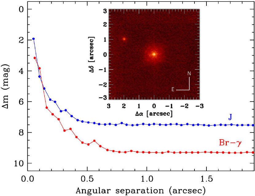
Figure 1.— Br-$\gamma$ Keck/NIRC2 AO image of KOI-490 shown along with the sensitivity curves in the $J$ (1.248 $\micron$) and Br-$\gamma$ (2.15 $\micron$) bands.

3.3. Centroid motion analysis

The very precise astrometry that can be obtained from the Kepler images enables a search for false positives that may be causing one or more of the signals in KOI-490, such as a background eclipsing binary. This can be done by measuring the location of the transit signals relative to the target by means of difference images, formed by subtracting an average of in-transit pixel values from out-of-transit pixel values. If a transit signal is caused by a stellar source, then the difference image will show that stellar source, and its location can be determined by pixel response function centroiding (Bryson et al., 2013). The centroid of an average out-of-transit image provides the location of KOI-490 because the object is well isolated. The centroid of the difference image is then compared to that of the out-of-transit image, which provides the location of the transit source relative to KOI-490.

The automatic pipeline processing of Kepler provides these offsets for each quarter in the Data Validation Reports, which are available through the CFOP Web site. For KOI-490.01 and KOI-490.03 the multi-quarter averages of the offsets indicate a position for the source of the transits that is consistent with the location of target. Based on the 1$\sigma$ uncertainties associated with those multi-quarter average offsets we adopted 3$\sigma$ radii of confusion for these two candidates of 0$\farcs$396 and 0$\farcs$603, respectively, within which the centroid motion analysis is insensitive to the presence of contaminating stars. As these limits are smaller than the separation of the 2$\farcs$2 companion reported earlier, that star cannot be the source of these transits.

For KOI-490.02 and KOI-490.04 the automatic fits performed by the Kepler pipeline failed, as indicated in the Data Validation Reports, so no centroid information is available for these candidates.

3.4. Stellar properties

The spectroscopic properties of KOI-490 were determined from an analysis of our Keck/HIRES spectrum. Our analysis was performed using the Stellar Parameter Classification (SPC) pipeline (Buchhave et al., 2012), which cross-correlates the observed spectrum against a large library of calculated spectra based on model atmospheres by R. L. Kurucz, and assigns stellar properties interpolating amongst those of the synthetic spectra providing the best match. This analysis gave $T_{\mathrm{eff}}=(4890\pm 50)$ K, $\log g=(4.61\pm 0.10)$, ${\rm[Fe/H]}=(-0.03\pm 0.08)$, and $v\sin i<2$ km s^-1. The measured radial velocity is $(-29.3\pm 1.0)$ km s^-1, and the effective temperature corresponds to a spectral type of K3 or K4.

The mass and radius of the star, along with other properties, were estimated by comparing the SPC parameters against a grid of Dartmouth isochrones (Dotter et al., 2008) with a $\chi^{2}$ procedure similar to that described by Torres et al. (2008). Because the stellar radius and age are largely determined by the surface gravity, and our $\log g$ determination provides a relatively weak constraint for KOI-490 given its uncertainty, we supplemented it with an estimate of the mean stellar density obtained by fitting the Kepler light curves of KOI-490.01, KOI-490.03, and KOI-490.04, on the assumption that they are true planets (justified below) and that they orbit the same star. The stellar parameters derived in this way are listed in Table 1, along with the inputs from SPC and the photometric mean density (posteriors shown in Figure 13). The inferred distance is based on the apparent $K_{s}$-band magnitude from 2MASS and a reddening estimate of $E(B-V)=(0.075\pm 0.030)$ from the Kepler Input Catalog (KIC; Brown et al., 2011).

Table 1Stellar properties of KOI-490.

Property	Value
$T_{\mathrm{eff}}$ (K)	$4890\pm 50$
$\log g$ (dex)	$4.61\pm 0.10$
${\rm[Fe/H]}$ (dex)	$-0.03\pm 0.08$
$v\sin i$ (km s-1)	$<2$
$\log_{10}[\rho_{\star}/($kg m${}^{-3})]$	$3.460_{-0.065}^{+0.031}$
$M_{\star}$ ($M_{\odot}$)	$0.770_{-0.028}^{+0.024}$
$R_{\star}$ ($R_{\odot}$)	$0.726_{-0.015}^{+0.018}$
$\log_{10}[L_{\star}/L_{\odot}]$	$-0.570_{-0.034}^{+0.036}$
$M_{V}$ (mag)	$6.53\pm 0.12$
$M_{K_{s}}$ (mag)	$4.21\pm 0.06$
Distance (pc)	$330\pm 10$
Age (Gyr)	$3.3_{-0.8}^{+5.8}$

Given these properties for KOI-490, we investigated whether the measured brightness and color of the 2$\farcs$2 neighbor reported earlier are consistent with those expected for a physically associated main-sequence star of later spectral type, i.e., one falling on the same Dartmouth isochrone as the primary. We find that an M4 or M5 dwarf with a mass around 0.20–0.21 $M_{\odot}$ would have approximately the right brightness compared to the primary, though its $J-K$ color would be about 0.16 mag bluer than we measure. However, given the uncertainties that may be expected in the theoretical flux predictions for cool stars (based here on PHOENIX model atmospheres implemented in the Dartmouth models), as well as variations in color that may occur in real stars due, e.g., to chromospheric activity, we consider the measured properties to be still consistent with a bound companion, although a chance alignment cannot be ruled out.

4. STATISTICAL VALIDATION

Transiting planet candidates require extra care to show that the periodic dips in stellar brightness are not astrophysical false positives, caused by other phenomena such as an eclipsing binary blended with the target (a “blend”). Because KOI-490 is a faint star ($V\approx 14.3$), it is challenging to confirm the planetary nature any of the candidates in this system dynamically, by measuring the Doppler shifts they induce on the host star. The alternative is to validate them statistically, showing that the likelihood of a true planet is far greater than that of a false positive. Rowe et al. (2014) followed this approach and reported the validation of two of the candidates, KOI-490.01 and KOI-490.03, based on the argument that most candidates in multiple systems can be shown statistically to have a very high chance of being true planets (Lissauer et al., 2012, 2014). These two planets received the official designations Kepler-167b and Kepler-167c. The validations relied in part on an examination of existing follow-up observations including spectroscopy and high-resolution imaging, and on an analysis of the flux centroids. The other two candidates in the system, KOI-490.02 and KOI-490.04, were not considered validated by Rowe et al. (2014) because the centroid information available was insufficient to determine whether the source of the photometric signals coincided with the location of the target, within errors. Additionally, the period of KOI-490.02 was not precisely known, since only one transit had occurred in the data at their disposal (Q1–Q10).

After the publication of the Rowe et al. (2014) work, AO imaging of KOI-490 was obtained that showed the presence of a 2$\farcs$2 companion that was unknown at the time (see § 3.2), and could possibly be the source of one of the signals. However, as pointed out earlier, the refined centroid information now available that includes Kepler observations from Q1–Q17 firmly rules out that the companion is causing the transits in KOI-490.01 and KOI-490.03, as it is well beyond the 3 $\sigma$ exclusion regions for these candidates (0$\farcs$396 and 0$\farcs$603, respectively; § 3.3). Thus, the validations of Rowe et al. (2014) stand.

We describe below our efforts to validate the other two candidates, KOI-490.02 (the snow-line candidate) and KOI-490.04, using the BLENDER technique (Torres et al., 2004, 2011; Fressin et al., 2012). This procedure has been applied successfully to the validation of many other transit candidates from Kepler (for recent examples see, e.g., Meibom et al., 2013; Ballard et al., 2013; Kipping et al., 2014; Torres et al., 2015; Jenkins et al., 2015). BLENDER addresses the possibility that the signals originate in an unseen background/foreground eclipsing binary (BEB) along the line of sight, a background or foreground star transited by a larger planet (BP scenario), or a stellar companion physically associated with the target that is in turn transited by another star or by a planet. These types of blends are usually the most difficult to rule out. The companions in the last two cases are usually close enough to the target as to be spatially unresolved. We refer to those hierarchical triple configurations as HTS or HTP, respectively, depending on the nature of the eclipsing object (star or planet). Other types of false positives that do not involve contamination by another object along the line of sight include grazing eclipsing binaries, and transits of a small star in front of a giant star. However, these cases can be easily ruled out as their signals would be inconsistent with the observed durations of transit ingress and egress for the two candidates.

Our validations with BLENDER follow closely the procedure described by Kipping et al. (2014) or Torres et al. (2015); the reader is referred to these sources for details of the methodology. In essence, BLENDER uses the shape of a transit light curve to rule out blend scenarios that would lead to the wrong shape for a transit. Large numbers of false positives of different kinds are simulated, and the synthetic light curves are then compared with the Kepler observations in a $\chi^{2}$ sense. Blends giving poor fits to the real data are considered to be excluded, and the ensemble of results places tight constraints on the detailed properties of viable blends including the sizes or masses of the objects involved, their brightness and colors, the linear distance between the background/foreground eclipsing pair and the KOI, and even the eccentricities of the orbits.

4.1. KOI-490.02, a Snow-line Candidate

Our simulations with BLENDER rule out background eclipsing binaries as the source of the signal. This is illustrated in Figure 2 (left panel), where we show the $\chi^{2}$ landscape in a representative cross-section of parameter space. The diagram shows the linear separation between the BEB and the target as a function of the mass of the primary star in the BEB. The only scenarios of this kind that provide acceptable fits to the Kepler light curve are those in which the main star of the binary is about twice as massive as KOI-490 (i.e., $M\sim 1.4~{}M_{\odot}$). These false positives occupy a narrow vertical strip on the lower right corner of the first panel in the figure (darker region contained within the white, 3$\sigma$ contour). However, all of these configurations result in a combined $r-K_{s}$ color index for the blend that is much bluer than the measured value for KOI-490 ($r-K_{s}=2.095\pm 0.027$), as indicated by the hatched blue region in the figure within which all blends have the wrong color. Furthermore, in these false positive configurations with F-type primaries the BEB is brighter than the target itself (see dashed green line). This conflicts with our spectroscopic classification of KOI-490 as an early K dwarf. We conclude that BEBs cannot mimic the transits of KOI-490.02 and simultaneously satisfy all observational constraints. This also rules out the 2$\farcs$2 companion as the source of the transits.

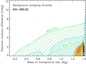
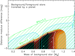
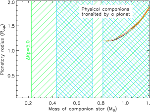
Figure 2.— Map of the $\chi^{2}$ surface (goodness of fit) for KOI-490.02 for three different blend scenarios, as labeled. Only blends within the solid white contours (darker shading) provide fits to the Kepler light curves that are within acceptable limits (3$\sigma$, where $\sigma$ is the significance level of the $\chi^{2}$ difference compared to a transiting planet model fit; see Fressin et al., 2012). Other concentric colored areas (lighter colors) represent fits that are increasingly worse (4 $\sigma$, 5 $\sigma$, etc.), which we consider to be ruled out. The hatched green areas indicate regions of parameter space where blended stars can be excluded if they are within 0$\farcs$43 of the target (half-width of the spectrometer slit), within five magnitudes in brightness (1% relative flux), and have a radial velocity differing from the target by 10 km s^-1 or more. In all of the above cases they would have been detected spectroscopically. Blends in the hatched blue areas can also be ruled out because they would be either too red (left) or too blue (right) compared to the measured $r-K_{s}$ color of KOI-490, by more than three times the measurement uncertainty. Left: BEB scenario. The vertical axis represents the linear distance between the eclipsing binary and the target ($D_{\rm BEB}-D_{\rm targ}$), cast for convenience in terms of the distance modulus difference $\Delta\delta=5\log(D_{\rm BEB}/D_{\rm targ})$. The dashed green line shown for reference is the locus of blends of equal apparent $K\!p$ brightness as the target. Middle: BP scenarios. As before, only blends that are brighter than the target (below the dashed green line) are able to mimic the light curve. The $r-K_{s}$ color constraint rules out most of those. Right: HTP scenario. The vertical axis now shows the size of the planet transiting the companion star, in units of Jupiter’s radius. All blends of this kind that provide acceptable fits to the light curve are too blue, and are therefore ruled out.

Blends involving background or foreground stars transited by a larger planet (BP scenario) are more easily able to match the transit shape and depth. This is shown in the middle panel of Figure 2, in which the permitted region is larger and accommodates chance alignments with stars between about 0.25 $M_{\odot}$ and 1.0 $M_{\odot}$. The spectroscopic constraint represented by the hatched green area excludes all such blends if the intruding stars have $\Delta K\!p<5$ mag and fall within the spectrometer slit (unless their spectral lines are blended with those of the target), as we would have detected them in our Keck/HIRES observation. Most other scenarios are also ruled out by the color constraint, but there is a narrow strip of viable blends in which the contaminating star has the same color (mass) as the target (see figure) so that it does not alter the combined $r-K_{s}$ index. These would then be near twin stars of our target, and they would have to be brighter than our nominal target because they are in the foreground. However, a star so similar to our target that is transited by a planet and is along the same line of sight but is brighter would effectively be our target, so we do not consider this as a false positive.

BLENDER indicates that physical companions eclipsed by another star (HTS scenario) invariably have the wrong shape for the transit, or produce secondary eclipses that are not seen in the Kepler data for KOI-490.02. Even in cases that show only a single eclipse due to a high eccentricity and a special orientation (Santerne et al., 2013) the properties of the primary of the eclipsing binary would be such that the overall brightness would make the binary detectable and/or make its color inconsistent with the measured color index of the target. These configurations are therefore easily ruled out. Physically associated stars transited by a larger planet (HTP scenario) can mimic the light curve only for a very narrow range of parameters, as illustrated in Figure 2, but those blends are all too blue because the companion needs to be even more massive than the target in order to produce the right shape for the transit, after accounting for dilution. We can thus exclude this category of blends completely.

In summary, our BLENDER simulations for KOI-490.02 combined with the observational constraints allow us to easily validate the candidate as a bona fide planet, ruling out as the source of the transits not only unseen background stars but also the known 2$\farcs$2 companion. A significant factor aiding in this process is the very high signal-to-noise ratio of the deep transits, thanks to which the shape is so well defined (particularly the ingress/egress phases) that very few configurations involving another star along the line of sight can match the Kepler photometry as well as a true transiting planet fit.

4.2. KOI-490.04

The transits of this candidate are much shallower than those of KOI-490.02, and as a result the constraint on the detailed shape of the light curve provided by the Kepler data is considerably weaker. Our BLENDER simulations indicate that false positives involving a bound companion eclipsed by a smaller star (HTS scenario) do not provide acceptable fits to the light curve, as in the previous case. However, not all blends corresponding to the BEB, BP, and HTP configurations can be ruled out. We illustrate this in Figure 3. For example, background eclipsing binaries that are more than five magnitudes fainter than the target in the Kepler band can match the shape of the light curve just as well as a model of a planet transiting the target, for a wide range of masses of the primary star of the binary between 0.6 $M_{\odot}$ and 1.4 $M_{\odot}$ (left panel). An even wider range of masses is permitted for background stars transited by a larger planet (BP, middle panel). Similarly, small stars physically bound to the target can mimic the light curve closely if transited by a planet of suitable size (right panel, HTP). Our follow-up observations may rule out some fraction of these blends, but not all of them.

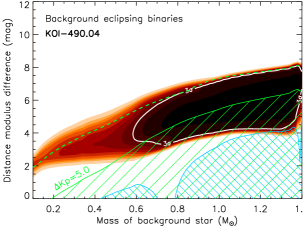
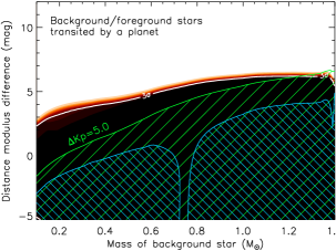
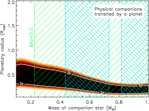
Figure 3.— Similar to Figure 2 for KOI-490.04, using the same color scheme. For this candidate all three scenarios feature blends that cannot be ruled out from the shape of the transits or constraints from our follow-up observations (darker areas not overlapping the hatched regions). The expected frequencies of each of these types of blends are estimated in the text.

To compute the expected rates of occurrence of each of these scenarios we followed the Monte Carlo procedure described by Torres et al. (2015), in which we simulated large numbers of blends and counted those that satisfy the constraints from BLENDER and the follow-up observations. The technique relies on the number densities of stars in the vicinity of KOI-490 (at Galactic latitude +9$\fdg$4), the estimated rates of occurrence of eclipsing binaries and transiting planets of various sizes and orbital periods, and other known properties of binary stars such as the distributions of their periods, eccentricities, mass ratios, etc. Details of these calculations may be found in the work cited above. We obtained estimated frequencies of $4.17\times 10^{-8}$ for the BEB scenario, $1.09\times 10^{-7}$ for BP, and $4.10\times 10^{-6}$ for HTP configurations. The total blend frequency is the sum of these, or $4.25\times 10^{-6}$. While this value may seem small in absolute terms, the a priori rate of occurrence of transiting planets of a given period and size (“planet prior”, PL) is also expected to be small. For a secure validation we require here that the “odds ratio” ${\rm PL}/(\rm{BEB}+\rm{BP}+\rm{HTP})$ be large enough so that the planet hypothesis is clearly favored over a false positive. Our estimate of the planet prior is $2.02\times 10^{-3}$, based on the number of known KOIs of similar size and period as the candidate. The resulting odds ratio is then 475, which corresponds to a confidence level of 99.79% that the signal is due to a bona fide planet. As this exceeds the 3$\sigma$ significance threshold typically adopted in BLENDER applications, it formally validates KOI-490.04 as a planet. There is, however, an important caveat to make: an implicit assumption for BLENDER is that there is no visible sign of a blend, whereas we know of the presence of the 2$\farcs$2 companion. Our BLENDER simulations in fact show (Figure 3) that a faint star such as this could well be causing the signal if transited by a larger planet, both as a physical companion to KOI-490 or as a background/foreground interloper. Under these circumstances the validation with BLENDER is not sufficient as it applies only to unseen sources, and we must seek alternate ways of ruling out the 2$\farcs$2 companion as the cause of the transit signals. This is successfully achieved through the use of asterodensity profiling, as described in §5.2.

5. LIGHT CURVE FITS

5.1. Joint fit to Kepler-167b and Kepler-167c

Planets Kepler-167b and Kepler-167c were both validated by Rowe et al. (2014) and new centroid information since that time excludes the possibility of these two objects orbiting the 2$\farcs$2 companion. This therefore establishes that Kepler-167b and Kepler-167c orbit the same star, namely the target star Kepler-167, to high confidence.

Fitting the transit light curve of a planet includes multiple parameters pertaining to the star itself, which may be described by the vector $\boldsymbol{\theta_{\star}}$. The vector $\boldsymbol{\theta_{\star}}$ contains the limb darkening coefficients describing the stellar intensity profile and the mean stellar density, $\rho_{\star}$. Since Kepler-167b and Kepler-167c orbit the same star, we can fit the transit lightcurves of both simultaneously, adopting a global $\boldsymbol{\theta_{\star}}$. By conditioning $\boldsymbol{\theta_{\star}}$ on the data describing both planets, we obtain a higher signal-to-noise measurement of these terms, which in turn leads to somewhat better precision on the local parameters, $\boldsymbol{\theta_{\mathrm{P}}}$, describing each planet (due to the inter-parameter covariances Carter et al. 2008).

In this work, we use the quadratic limb darkening law with the optimal parameterization ($q_{1}$ & $q_{2}$) described by Kipping (2013b). The light curves are generated with the Mandel & Agol (2002) algorithm using 30-point resampling to account for those point which are long-cadence, as described in Kipping (2010). Quarter-to-quarter contamination factors are accounted for, using the “CROWDSAP” header information in the raw fits files via the method described by Kipping & Tinetti (2009). A blending factor affecting all quarters due to the 2$\farcs$2 companion is also accounted for via this method.

For the global blending factor, we convert the $J$ and $K_{s}$ colors observed in the NIRC2 AO images to a Kepler bandpass magnitude using the fifth-order polynomial relation in Appendix A of Howell et al. (2012). Assuming either a dwarf or a giant leads to the same result (within the estimated uncertainty) of $K\!p=19.0\pm 0.1$. Assuming Gaussian errors on the $J$ and $K_{s}$ colors from AO and adding in quadrature an extra Gaussian uncertainty reflecting the 0.05 magnitude error in the Howell et al. (2012) relation, we estimate a blending factor of $\log\beta=(-1.976\pm 0.036)$, where $\beta$ is the flux ratio between the target and the companion in the Kepler bandpass. This is treated as a normal prior in our fits and added to the $\boldsymbol{\theta_{\star}}$ vector, since it is a term affecting all of the planets. The parameters and priors used are listed in Table 2, with the $\boldsymbol{\theta_{\star}}$ plus two sets of $\boldsymbol{\theta_{\mathrm{P}}}$ parameters giving a total of 12 free parameters in our model.

Table 2 Priors for the joint fit to KOI-490.01 & KOI-490.03. $\mathcal{J}$ is a Jeffreys prior, $\mathcal{N}$ is a normal and $\mathcal{U}$ is uniform.

Description	Symbol	Prior
Global parameters	$\boldsymbol{\theta_{\star}}$
Mean stellar density [kg m-3]	$\rho_{\star}$	$\mathcal{J}[10,10^{6}]$
Limb darkening coefficient 1	$q_{1}$	$\mathcal{U}[0,1]$
Limb darkening coefficient 2	$q_{2}$	$\mathcal{U}[0,1]$
Log of the blending flux ratio	$\log_{10}\beta$	$\mathcal{N}(-1.976,0.036)$
Local parameters	$\boldsymbol{\theta_{\mathrm{P}}}$
Ratio-of-radii	$(R_{P}/R_{\star})$	$\mathcal{U}[0,1]$
Impact parameter	$b$	$\mathcal{U}[0,2]$
Orbital period [d]	$P$	$\mathcal{U}[\bar{P}-0.1,\bar{P}+0.1]$
Time of transit minimum [d]	$\tau$	$\mathcal{U}[\bar{\tau}-0.1,\bar{\tau}+0.1]$

Fits were achieved using the multimodal nested sampling algorithm MultiNest (Feroz & Hobson, 2008; Feroz et al., 2009) with 4000 live points and a target efficiency set to 0.1. The eccentricities of Kepler-167b and Kepler-167c are assumed to be zero in the fits. Multi-planet Kepler systems are known to have low eccentricities, with Van Eylen & Albrecht (2015) finding a Rayleigh distribution with $\sigma_{e}=0.049\pm 0.013$ describes the overall population. Moreover, Kepler-167b and Kepler-167c orbit the same star with orbital periods of 4.4 d and 7.4 d, placing them in close proximity to both the star and each other. We therefore expect these planets to be particularly likely to have near-zero eccentricity, from a dynamical perspective.

Rather than describe the posteriors found for each parameter, we focus here on the term $\rho_{\star}$, since the others will be superseded by the global fits performed later. The posterior distribution for $\log_{10}(\rho_{\star})$ (it is more appropriate to discuss the log since we invoked a Jeffreys prior) yields $\log_{10}[\rho_{\star}($kg m${}^{-3})]=3.446_{-0.098}^{+0.034}$ and is plotted in Figure 4. This may be compared to the density expected by iscohrone-matching using the effective temperature, metallicity and surface gravity found using SPC. Drawing random samples from three normal distributions describing each and finding the nearest Dartmouth isochrone each time, we derive a wholly independent stellar density for Kepler-167 of $\log_{10}[\rho_{\star}($kg m${}^{-3})]=3.455_{-0.016}^{+0.015}$. The close agreement between the two is further evidence that Kepler-167b and Kepler-167c orbit the target star, although their validation (Rowe et al., 2014) was performed independent of this fact.

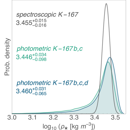
Figure 4.— Posterior distribution of the mean stellar density of Kepler-167 conditioned on the transits of Kepler-167b & c (green) and Kepler-167b, c & d (blue). We only assume that the planets orbit the same star and have circular orbits. For comparison, the posterior derived using isochrone matching of the SPC stellar atmosphere constraints is shown in black.

5.2. Two Fits for KOI-490.04

From the validation discussion in § 4, it was established that KOI-490.04 does not orbit an unseen companion to 3 $\sigma$ confidence, but may still orbit the seen 2$\farcs$2 companion. Here, we perform two fits to explore these two hypotheses.

In hypothesis A ($\mathcal{H}_{A}$), we assume that KOI-490.04 orbits the target star, which we have established also hosts Kepler-167b and Kepler-167c. The posterior distribution of the light curve derived stellar density from the fit in § 5.1 becomes the prior for the same term in this hypothesis. Note that this distribution does not invoke any information from the spectroscopic analysis. All of the other parameters retain the same priors listed in Table 2. Specifically, the limb darkening parameters are treated as free again, since these were poorly constrained from the previous fit.

For $\mathcal{H}_{A}$, we relax the assumption of a circular orbit. Since KOI-490.04 is further from both the star and the other two planets ($P\sim 21.8$ d), higher eccentricities are possible. In this hypothesis though, KOI-490.04 belongs to a typical Kepler multi-planet system and thus we adopt the eccentricity distribution derived by Van Eylen & Albrecht (2015); a Rayleigh distribution with $\sigma_{e}=0.049$. The prior for the argument of periapsis becomes increasingly non-uniform as eccentricity diverges from zero, due to a geometric effect (see Kipping 2014a). Nevertheless, a uniform prior is reasonable in this case given the low-eccentricity nature of the Van Eylen & Albrecht (2015) distribution.

In hypothesis B ($\mathcal{H}_{B}$), we assume that KOI-490.04 orbits the 2$\farcs$2 companion. Here, the object can no longer be considered to belong to a multi-planet system, since Kepler-167b and Kepler-167c orbit a different star now. Therefore, the potential for high eccentricities becomes even greater and we consider the object to follow a Beta distribution calibrated to the population of radial velocity planets with orbital periods less than one year, as described by Kipping (2013a) ($\sim\mathrm{Beta}[0.694,3.252]$). In this case, the geometric bias due to the transit probability is more significant and requires accounting for. We therefore use the ECCSAMPLES code described by Kipping (2014a) to modify the Beta prior to a prior conditioned on the fact we know this object is transiting. However, rather than directly sampling from the prior, we penalized the likelihood function appropriately to improve computational efficiency. Additionally, since the star is different to Kepler-167, the mean stellar density follows an uninformative Jeffreys prior, $\mathcal{J}[1,10^{9}]$ kg m^-3. Finally, the blending prior is flipped to consider the blend source being Kepler-167.

We fitted both models using MultiNest, which returns the Bayesian evidence, $\mathcal{Z}$, enabling Bayesian model selection between the two. Note that this is essentially a more advanced treatment of using the photo-blend effect (Kipping, 2014b) employed in validating several candidates by Torres et al. (2015). Bayesian model selection favors hypothesis A with $\Delta(\log\mathcal{Z})=(5.57\pm 0.10)$. Given that only two hypothesis exist, the statistical significance of hypothesis A being the preferred model is 2.9 $\sigma$. We therefore use the photo-blend effect to show that KOI-490.04 orbits the target star to 99.6% confidence.

However, in hypothesis B, the mean stellar density required to explain the data is $\log_{10}[\rho_{\star}($kg m${}^{-3})]=3.49_{-0.28}^{+0.16}$. This would make the companion star of similar spectral type to that of Kepler-167. This essentially excludes the possibility of a bound binary, since the AO companion could not be 5 magnitudes fainter in this case. If this were a chance alignment of a background star, we would still expect the host star to have a similar color to the primary. However, $J-K_{s}$ of Kepler-167 is $(0.60\pm 0.03)$ whereas the AO companion has $J-K_{s}=(0.94\pm 0.05)$. Reddening can not explain such a large difference either and thus we conclude that hypothesis B is even less likely than indicated by the formal Bayesian evidence comparison. We therefore conclude that KOI-490.04 orbits Kepler-167 to a confidence exceeding 3 $\sigma$ and thus may be considered a “validated” planet, designated Kepler-167d.

Since hypothesis A invokes the posterior of $\rho_{\star}$ from the earlier joint fit of Kepler-167b & c as a prior, the eccentricity of Kepler-167d is constrained without any use of stellar evolution or atmosphere models. This demonstrates perhaps the first applied example of Multibody Asterodensity Profiling (MAP), proposed by Kipping et al. (2012). However, we find that the light curve of Kepler-167d is of insufficient data quality to provide a meaningful improvement on the eccentricity constraint over the prior. Specifically, in hypothesis A, the eccentricity posterior closely resembles the prior (see Figure 5) and the credible intervals on $e$ change from $0.058_{-0.029}^{+0.036}$ (the prior) to $0.055_{-0.027}^{+0.035}$ (the posterior).

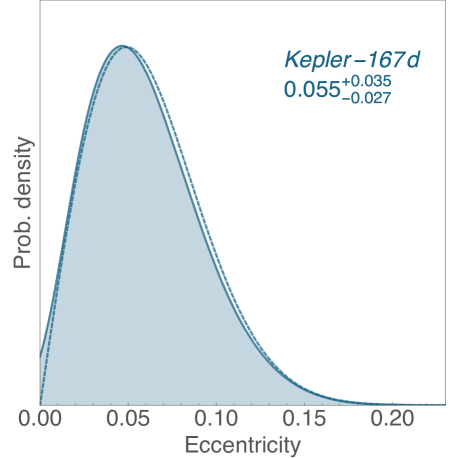
Figure 5.— Posterior distribution (solid) of the orbital eccentricity of Kepler-167d, with comparison to the prior (dashed) describing Kepler multis (Van Eylen & Albrecht, 2015). The eccentricity is constrained by the comparison of the transit light curve shape of Kepler-167d to the $\rho_{\star}$ constraint from the earlier joint fit of Kepler-167b & c.

5.3. Parameters and Eccentricity of Kepler-167e

Having established that Kepler-167b, Kepler-167c and Kepler-167d orbit the same star, we perform a new global fit adopting a common $\boldsymbol{\theta_{\star}}$ for the parent star. Since the eccentricity of Kepler-167d is inferred to be consistent with a low eccentricity prior, we assume the orbit is nearly circular in this global fit. Including the third planet provides a modest improvement in the constraint on the mean stellar density, as expected. This may be seen in Figure 4 where the constraint tightens up to $\log_{10}[\rho_{\star}($kg m${}^{-3})]=3.460_{-0.065}^{+0.031}$. We use this posterior on the mean density as an additional constraint for the fundamental stellar parameters through isochrone matching, as described earlier in § 3.4. The full set of posteriors from this fit are shown in Figure 11 and are available for download at this URL.

Using the new revised isochrone modeling and the ratio-of-radii posteriors from this three-planet joint fit, we infer our best-estimate of the radii of planets Kepler-167b, c & d to be $R_{b}=1.615_{-0.043}^{+0.047}$ $R_{\oplus}$, $R_{c}=1.548_{-0.048}^{+0.050}$ $R_{\oplus}$ and $R_{d}=1.194_{-0.048}^{+0.049}$ $R_{\oplus}$. The maximum likelihood light curve models for the planets in the Kepler-167 system are shown in Figure 6.

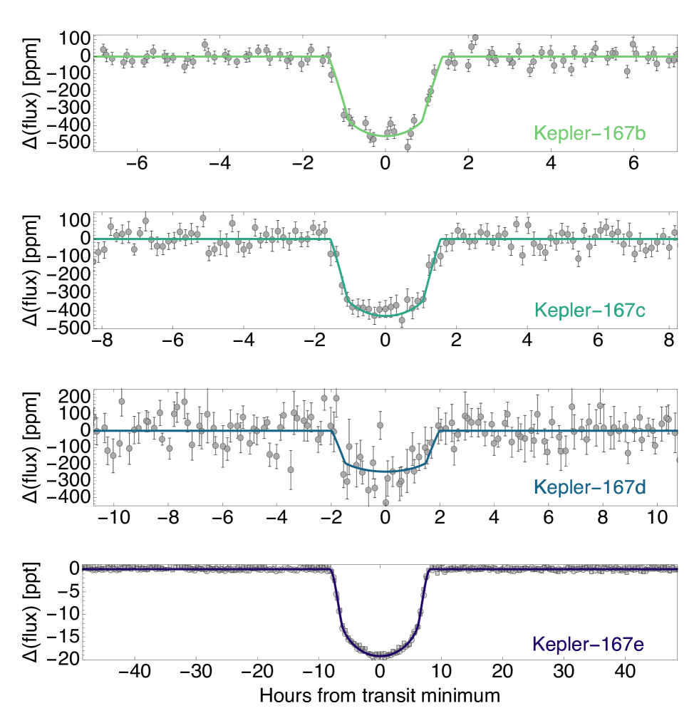
Figure 6.— Folded transit light curves of Kepler-167b, Kepler-167c, Kepler-167d and Kepler-167e. For the upper three, data (gray points) are binned to a 10 minute cadence. Light curve of Kepler-167e uses 30 minute binning and uses circles to denote the first transit (Q4) and squares to denote the second transit (Q16). Note that all of the transits were fitted using the original unbinned data.

Note that despite using three transiting planets, the limb darkening coefficients are poorly constrained returning only marginally different posteriors from the priors. Specifically, we measure $q_{1}=0.63_{-0.30}^{+0.26}$ and $q_{2}=0.17_{-0.10}^{+0.18}$.

We now turn our attention to the outer planet, Kepler-167e, which was validated earlier to orbit the target star (see § 4.1). We first verified that the period of 1071 d is the correct one, by inspecting the raw light curve around integer ratios of the candidate period. Given the depth of 1.6%, even a simple visual inspection excludes this possibility. As was done by Kipping et al. (2014), we also verified that the shape of the two transit events observed are consistent which is also visually evident in Figure 6. Basic parameters derived from two independent fits of each event reveal that the events are consistent, as shown in Table 3 (note that the first transit is long-cadence and the second, short).

Table 3 Comparison of the basic transit parameters of Kepler-167e when epochs 1 & 2 are fitted independently. The last three differ by 0.9, 1.2 & 1.2 $\sigma$ respectively.

Parameter	Epoch 1	Epoch 2
$\tau$ [BKJDUTC-2,455,000]	$253.28698_{-0.00043}^{+0.00042}$	$1324.51928_{-0.00045}^{+0.00044}$
$(R_{P}/R_{\star})$	$0.1265_{-0.0011}^{+0.0014}$	$0.1284_{-0.0016}^{+0.0015}$
$T_{14}$ [hours]	$16.241_{-0.079}^{+0.090}$	$16.114_{-0.071}^{+0.070}$
$T_{23}$ [hours]	$12.48_{-0.18}^{+0.14}$	$12.15_{-0.20}^{+0.20}$

Given that Kepler-167e is a much longer orbital period planet than the other three, the potential for an eccentric orbit is much higher both a-priori as a member of the long-period planet sample (Kipping, 2013a) and dynamically since it is essentially decoupled from the other three.

We treat the posterior distribution for the mean stellar density of the Kepler-167b, c & d joint fit as a prior in the fits of planet e. Although there is a weak constraint on the limb darkening coefficients, we consider the information too weak to be worth including and thus treat the limb darkening coefficients as independent and free. Therefore the priors largely follow those listed in Table 2, except for $\rho_{\star}$.

It is also crucial to include the orbital eccentricity and argument of periapsis. Given the potential for a large eccentricity, the geometric bias effect described by Kipping (2014a) becomes pronounced and must be accounted for. As was done in hypothesis B of the KOI-490.04 fits, we use the geometry-corrected Beta prior from Kipping (2014a) via a likelihood penalization implementation, adopting Beta shape parameters calibrated to the long-period ($>1$ year) radial velocity exoplanet catalog (Kipping, 2013a) (specifically $\sim\mathrm{Beta}[1.12,3.09]$).

Unlike the case of Kepler-167d, the light curve plus stellar density prior does provide a more constraining posterior on the derived eccentricity than the prior. As shown in Figure 7, the orbit is measured to be close to circular, with $e=0.062_{-0.043}^{+0.104}$. Using the posteriors for the fundamental stellar parameters derived using SPC along with the Kepler-167b, c & d $\rho_{\star}$ constraint plus isochrone matching, we estimate that Kepler-167e is $\sim 10$% smaller than Jupiter at $10.15_{-0.23}^{+0.24}$ $R_{\oplus}$.

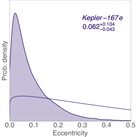
Figure 7.— Posterior distribution (solid) of the orbital eccentricity of Kepler-167e, with comparison to the prior (dashed) describing long-period transiting planets (Kipping, 2014a). The eccentricity is constrained by the comparison of the transit light curve shape of Kepler-167e to the $\rho_{\star}$ constraint from the earlier joint fit of Kepler-167b, c & d.

The posteriors from the fit of Kepler-167e are shown in Figure 12 and are available at this URL. The median and 68.3% credible intervals for the basic parameters of Kepler-167b, c, d & e are shown in Table 4.

Table 4Final parameter estimates for the planets orbiting Kepler-167. ^‡ = fixed; ^† = assuming a Bond albedo similar to Jupiter of 0.34 (whereas we simply adopt 0 for the other cases due to the uncertainty in what kind of planet they are, as shown in Figure 10). ^∗ = equivalent semi-major axis of the planet if it orbited the Sun with $e=0$ and insolation level $S_{\mathrm{eff}}$.

Parameter	Kepler-167b	Kepler-167c	Kepler-167d	Kepler-167e
Fitted parameters
$\log_{10}[\rho_{\star}$ (kg m-3)]	$3.460_{-0.065}^{+0.031}$	$3.460_{-0.065}^{+0.031}$	$3.460_{-0.065}^{+0.031}$	$3.460_{-0.065}^{+0.031}$
$q_{1}$	$0.63_{-0.30}^{+0.26}$	$0.63_{-0.30}^{+0.26}$	$0.63_{-0.30}^{+0.26}$	$0.452_{-0.063}^{+0.072}$
$q_{2}$	$0.17_{-0.10}^{+0.18}$	$0.17_{-0.10}^{+0.18}$	$0.17_{-0.10}^{+0.18}$	$0.463_{-0.053}^{+0.062}$
$\log_{10}\beta$	$-1.976\pm 0.036$	$-1.976\pm 0.036$	$-1.976\pm 0.036$	$-1.976\pm 0.036$
$(R_{P}/R_{\star})$	$0.02036_{-0.00032}^{+0.00034}$	$0.01952_{-0.00044}^{+0.00042}$	$0.01507_{-0.00052}^{+0.00050}$	$0.12810_{-0.00093}^{+0.00091}$
$b$	$0.17_{-0.12}^{+0.18}$	$0.25_{-0.13}^{+0.13}$	$0.474_{-0.063}^{+0.076}$	$0.233_{-0.068}^{+0.049}$
$P$ [days]	$4.3931632_{-0.0000045}^{+0.0000046}$	$7.406114_{-0.000011}^{+0.000012}$	$21.803855_{-0.000119}^{+0.000078}$	$1071.23228_{-0.00056}^{+0.00056}$
$\tau$ [BKJDUTC-2,455,000]	$831.78317_{-0.00036}^{+0.00034}$	$552.15774_{-0.00084}^{+0.00129}$	$669.7934_{-0.0018}^{+0.0015}$	$253.28699_{-0.00040}^{+0.00039}$
$e$	$0^{\ddagger}$	$0^{\ddagger}$	$<0.12$	$0.062_{-0.043}^{+0.104}$
$\omega$ [rads]	-	-	-	$3.5_{-2.9}^{+2.6}$
Other transit parameters
$(a/R_{\star})$	$14.33_{-0.69}^{+0.35}$	$20.30_{-0.98}^{+0.49}$	$41.7_{-2.0}^{+1.0}$	$560_{-15}^{+11}$
$u_{1}$	$0.63_{-0.20}^{+0.15}$	$0.63_{-0.20}^{+0.15}$	$0.63_{-0.20}^{+0.15}$	$0.915_{-0.019}^{+0.020}$
$u_{2}$	$0.14_{-0.25}^{+0.28}$	$0.14_{-0.25}^{+0.28}$	$0.14_{-0.25}^{+0.28}$	$-0.243_{-0.038}^{+0.040}$
$i$ [∘]	$89.33_{-0.80}^{+0.47}$	$89.30_{-0.43}^{+0.36}$	$89.352_{-0.140}^{+0.090}$	$89.9760_{-0.0052}^{+0.0070}$
$T_{14}$ [hours]	$2.350_{-0.035}^{+0.035}$	$2.746_{-0.061}^{+0.096}$	$3.582_{-0.073}^{+0.131}$	$16.13_{-0.34}^{+0.44}$
$T_{23}$ [hours]	$2.249_{-0.033}^{+0.035}$	$2.630_{-0.064}^{+0.098}$	$3.440_{-0.077}^{+0.137}$	$12.29_{-0.33}^{+0.38}$
$T_{12}\simeq T_{34}$ [mins]	$2.89_{-0.086}^{+0.342}$	$3.36_{-0.14}^{+0.37}$	$4.09_{-0.27}^{+0.49}$	$115.9_{-3.7}^{+3.7}$
Physical parameters
$R_{P}$ [$R_{\oplus}$]	$1.615_{-0.043}^{+0.047}$	$1.548_{-0.048}^{+0.050}$	$1.194_{-0.048}^{+0.049}$	$10.15_{-0.23}^{+0.24}$
$a$ [AU]	$0.0483_{-0.0025}^{+0.0017}$	$0.0684_{-0.0035}^{+0.024}$	$0.1405_{-0.0071}^{+0.0050}$	$1.890_{-0.067}^{+0.058}$
$T_{\mathrm{eq}}$ [K]	$914_{-16}^{+26}$	$768_{-14}^{+21}$	$536.0_{-9.6}^{+14.4}$	$130.9_{-3.0}^{+2.0}$ †
$S_{\mathrm{eff}}$ [$S_{\oplus}$]	$115.8_{-8.0}^{+13.0}$	$57.7_{-4.0}^{+6.5}$	$13.68_{-0.95}^{+1.54}$	$0.0739_{-0.0091}^{+0.0047}$
$a_{\mathrm{eff}}^{*}$ [AU]	$0.0929_{-0.0048}^{+0.0034}$	$0.1316_{-0.0068}^{+0.0048}$	$0.270_{-0.014}^{+0.010}$	$3.64_{-0.13}^{+0.12}$
$M_{\mathrm{forecast}}$ (1 $\sigma$ interval)	$2.4M_{\oplus}$–$6.3M_{\oplus}$	$2.2M_{\oplus}$–$5.8M_{\oplus}$	$1.2M_{\oplus}$–$2.9M_{\oplus}$	$0.3M_{\mathrm{J}}$–$50M_{\mathrm{J}}$

6. DISCUSSION

6.1. A Transiting Jupiter Analog

Kepler-167e appears to be the first example of a transiting Jupiter analog, as defined by its size ($0.91$ $R_{\mathrm{J}}$), low eccentricity ($e=0.06_{-0.04}^{+0.10}$) and location beyond the snow-line (see Figure 8). Although Jupiter analogs have been found via other methods (e.g. see Rowan et al. 2015), the geometric biases affecting the transit method make it highly unfavorable for discovering such worlds.

Kepler-167e has an a priori transit probability of $\simeq 0.18$%. Combined with the $\eta_{\jupiter}\simeq 3$% occurrence rate of Jupiter analogs (Rowan et al., 2015), one should expect $\mathcal{O}[10]$ transiting examples to exist amongst the $\sim 200,000$ stars observed by Kepler. However, only those objects just beyond the snow-line and orbiting later than Solar-type stars will have a chance to produce the two transits needed to resolve the orbital period. Consequently, it is possible that Kepler-167e could be the only transiting Jupiter analog for which we can precisely measure the period until the next generation of surveys.

The fact that Kepler-167e is transiting offers the opportunity to probe the atmosphere of a genuine Jupiter analog (Dalba et al., 2015), which has thus far been impossible. Whilst Kepler-167 is relatively faint in the $V$ band at 14.3, the fact that this is a late-type star means the planet may be characterizable toward the near- and mid-infrared bandpasses, where the $K$-band magnitude is 11.8. This fact, combined with the very deep transit depth of 1.6%, makes atmospheric characterization a challenging, but not impossible, task.

As was done by Kipping et al. (2014), we used the Kennedy & Kenyon (2008) predictions for the time-evolving snow-line of a $\sim 0.8$ $M_{\odot}$ star to estimate that Kepler-167e’s present location corresponds to the snow-line after $\sim 800,000$ years. This time is less than the median lifetimes of protoplanetary disks of Solar-type stars (e.g., Strom et al., 1993; Haisch et al., 2001) and since disk lifetimes scale as $M_{\star}^{-1/2}$ (Yasui et al., 2012), Kepler-167e could have formed at its present location. Unlike Kepler-421b (Kipping et al., 2014), which was “near” the snow-line, Kepler-167e is comfortably beyond it for the majority of the disk lifetime.

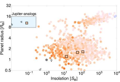
Figure 8.— Catalog of known transiting exoplanets with the color depicting the peak wavelength color of the parent star. Solar System worlds are shown with black symbols and the Kepler-167 planets with squares. The blue-box depicts Jovian-sized planets beyond the snow-line ($\sim 0.25$ $S_{\oplus}$), with Kepler-167e being the first transiting exoplanet to fill this space. Data comes from the Exoplanet Orbit Database (Wright et al., 2011).

6.2. Could Kepler-167e be a brown dwarf?

With a radius close to that of Jupiter, Kepler-167e is a member of the so-called “degenerate worlds” class, where the mass-radius relation is nearly flat (Chen & Kipping, 2016). This class encompasses a diverse range of masses, from that of Saturn to the most massive brown dwarfs. On this basis, Kepler-167e’s radius is consistent with being either a brown dwarf or a Jovian-like planet. As argued by Chen & Kipping (2016), the division between brown dwarfs and gas giants is somewhat contrived, with both belonging to a continuum. Nevertheless, we evaluate the possibility that Kepler-167e’s mass is greater than the 13 $M_{\mathrm{J}}$ canonical threshold (Spiegel et al., 2011) here.

Using the radius-to-mass probabilistic forecasting code of Chen & Kipping (2016), our radius samples can be converted to predicted masses. Being a degenerate world, this unsurprisingly returns a very broad distribution, with the 68.3% credible interval spanning 0.3 $M_{\mathrm{J}}$ to 50 $M_{\mathrm{J}}$. We find that the probability of the mass being less than the hydrogen-burning limit to be 97.4%, indicating that Kepler-167e is very unlikely to be a star. Moreover, we find 1.33 times more samples below the 13 $M_{\mathrm{J}}$ threshold than above it, implying a slight preference for a Jupiter-like object.

This estimate can be improved by including a suitable occurrence rate prior, for which we here use Cumming et al. (2008) power-law of occurrence rate $\sim M^{-0.31}$. This adds further weight to the Jupiter-like scenario with an odds ratio of 4.28. We therefore estimate that Kepler-167e is four times more likely to be a Jupiter-like planet than a brown dwarf.

It may be possible for observers exclude the brown dwarf hypothesis using radial velocities. If Kepler-167e is a brown dwarf, then the radial velocity amplitude would be $K\geq 316_{-11}^{19}$ m s^-1. In contrast, the (broad) forecasted radial velocity amplitude is $\log_{10}[K\,(\mathrm{m}\,\mathrm{s}^{-1})]=2.32_{-1.47}^{+0.75}$ (i.e. $\sim 211$ m s^-1).

6.3. Multibody Asterodensity Profiling

The eccentricity of Kepler-167e is measured purely using the transit shapes of the orbiting planets, representing a first for the field. In all previous cases, independent information constraining the mean stellar density was used, such as spectroscopic + isochrone analysis (Dawson & Johnson, 2012), asteroseismology (Sliski & Kipping, 2014) or flicker (Kipping et al., 2014).

The eccentricity of a transiting planet can be measured using asterodensity profiling (Kipping, 2014b), specifically via the photo-eccentric effect (Dawson & Johnson, 2012). This essentially compares the light curve derived stellar density (related to the $T_{14}$ and $T_{23}$ transit durations) to that derived via some independent method. Although eccentricity is the dominant effect, for Kepler-167 the photo-blend effect is in play too, due to the AO detected companion.

Whilst the most common and accessible method to get an independent mean stellar density is spectroscopy combined with isochrone modeling, this approach essentially makes the unrealistic assumption of zero-model error. Multibody Asterodensity Profiling (Kipping et al., 2012) was conceived with the idea of comparing the light curves of planets orbiting the same star against one another, to obviate the need to ever go through evolutionary models. In the case of multiple eccentric planets, the inverse problem is quite challenging but the compact, inner three planets of Kepler-167 are likely on near-circular orbits, providing a so-called “stellar anchor” we can use to characterize the star. This inference is then used to measure the eccentricity of the outer planet, which a priori could be much more eccentric.

We are able to measure the eccentricity to be $e=0.06_{-0.04}^{+0.10}$, which further supports the case that Kepler-167e is a Jupiter analog. Critically, we emphasize that this measurement used nothing more than the Kepler photometric time series of a $14^{\mathrm{th}}$ magnitude star and a single night of AO imaging on a 10 m telescope. As a comparison, HD 32963b is a recently discovered Jupiter analog found using radial velocities (Rowan et al., 2015) for which 199 nights of precise radial velocities on a 10 m class telescope led to the comparable constraint of $e=(0.07\pm 0.04)$, in spite of the fact that HD 32963 is six and a half magnitudes brighter than Kepler-167. However, the transit method does have the major drawback that transiting Jupiter analogs are far less numerous than their non-transiting counterparts.

6.4. System Architecture

All three inner planets orbit interior to the inner edge of the habitable-zone (Kopparapu et al., 2013) and are unlikely to be interesting from an astrobiological perspective. The architecture of the Kepler-167 system is curious, with a compact multi followed by a large cavity of transiting planets and then an outer Jupiter analog (see Figure 9). Thus, Kepler-167 resembles a fusion of the compact Kepler multis and the classic Solar System. Since transit surveys have a very poor sensitivity to long-period planets like Kepler-167e (planet yield $\sim P^{-5/3}$; Beatty & Gaudi 2008), it is plausible that Kepler-167e-like planets are found frequently in the Kepler compact multis. A radial velocity survey targeting the bright Kepler multis would be able to resolve this question.

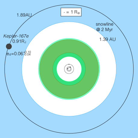
Figure 9.— Schematic illustrating the scale of the Kepler-167 system. Planet sizes are scaled relative to the key, rather than the orbital distances in order to make them visible. The four known planets display remarkable coplanarity and near-circular orbits with the habitable-zone (Kopparapu et al., 2013) notably devoid of transiting planets.

Additional non-transiting planets could reside in the Kepler-167 cavity, although the known four planets display remarkable coplanarity and low eccentricities, suggestive of a dynamically cold system. Amongst the inner planets, the planet sizes increase as one approaches the parent star. Using the Chen & Kipping (2016) mass-radius model, we estimate that the inner two planets are most likely gaseous worlds whilst the outer planet is most likely rocky (see Figure 10). Whilst this pattern ostensibly jars our anthropocentric prior, as well as the expected outcome of photo-evaporation (Lopez & Fortney, 2013), Ciardi et al. (2013) find that there is no preferential ordering of compact Kepler multis for planets $R\lesssim 3R_{\oplus}$.

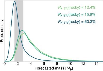
Figure 10.— Forecasted masses for the planets Kepler-167b (green), Kepler-167c (turquoise) and Kepler-167d (blue) using our radii posterior samples and the radius-to-mass forecasting model of Chen & Kipping (2016). Gray region denotes the 1 $\sigma$ confidence interval of the transition from rocky to gaseous worlds found by Chen & Kipping (2016).

The Kepler-167 system teases the possibility that compact multis may plausibly harbor distant Jupiter analogs, inviting the community to pursue this question with current and future facilities. Moreover, whilst Kepler-167 is not a bright star, transiting Jupiter analogs represent an important new class of targets in the on-going campaigns to characterize the atmospheres of alien worlds. Discovering members of this population around brighter stars is a challenging but likely rewarding task for future missions.

Appendix:Posterior Distributions

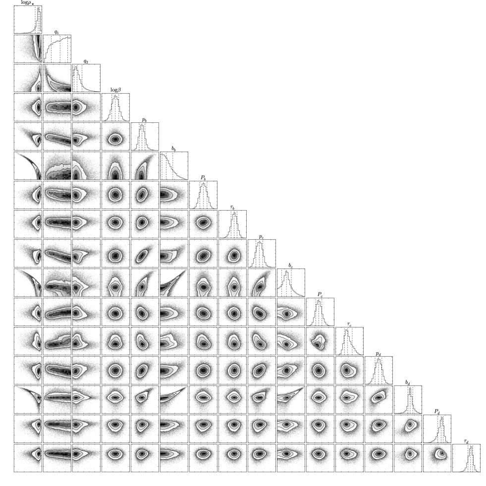
Figure 11.— Triangle plot of the posterior distributions of the 16 parameters explored in the joint fit of Kepler-167b, c & d. Contours mark the 0.5, 1.0, 1.5 & 2.0 $\sigma$ confidence intervals and dashed lines on the histograms mark the median and surrounding 1 $\sigma$ confidence interval. Posteriors may be downloaded at this URL.

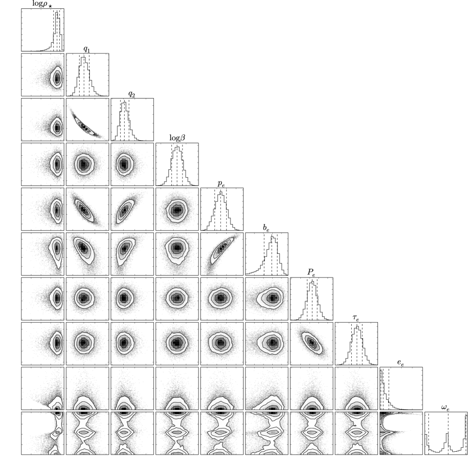
Figure 12.— Triangle plot of the posterior distributions of the 10 parameters explored in the fit of Kepler-167e. Contours mark the 0.5, 1.0, 1.5 & 2.0 $\sigma$ confidence intervals and dashed lines on the histograms mark the median and surrounding 1 $\sigma$ confidence interval. Posteriors may be downloaded at this URL.

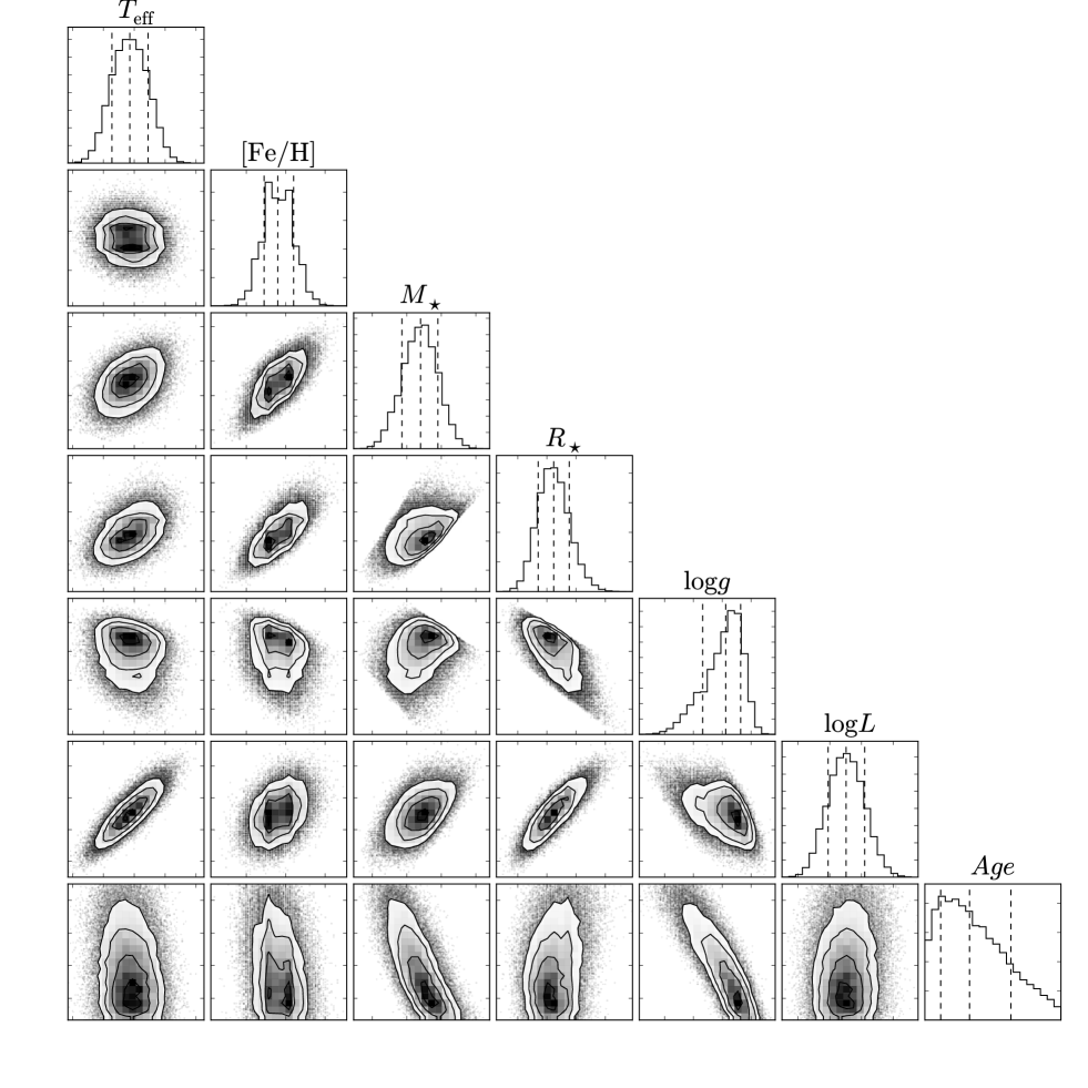
Figure 13.— Triangle plot of the posterior distributions of fundamental stellar parameters using SPC plus Dartmouth isochrones. Contours mark the 0.5, 1.0, 1.5 & 2.0 $\sigma$ confidence intervals and dashed lines on the histograms mark the median and surrounding 1 $\sigma$ confidence interval. Posteriors may be downloaded at this URL.

References

- Akeson et al. (2013) Akeson, R. L., Chen, X., Ciardi, D. et al. 2013, PASP, 125, 989
- Ballard et al. (2013) Ballard, S., Charbonneau, D., Fressin, F. et al. 2013, ApJ, 773, 98
- Barclay et al. (2013) Barclay, T., Rowe, J. F., Lissauer, J. J. et al. 2014, Nature, 494, 452
- Batygin & Laughlin (2015) Batygin, K. & Laughlin, G. 2015, PNAS, 112, 4214
- Beatty & Gaudi (2008) Beatty, T. G. & Gaudi, S. B., 2008, ApJ, 686, 1302
- Brown et al. (2011) Brown, T. M., Latham, D. W., Everett, M. E., & Esquerdo, G. A., AJ, 142, 112
- Bryson et al. (2013) Bryson, S. T., Jenkins, J. M., Gilliland, R. L., et al. 2013, PASP, 125, 889
- Buchhave et al. (2012) Buchhave, L. A., Latham, D. W., Anders, J. et al. 2012, Nature, 486, 375
- Carter et al. (2008) Carter, J. A., Yee, J. C., Eastman, J. et al., 2008, ApJ, 689, 499
- Chen & Kipping (2016) Chen, J. & Kipping, D. M., 2016, submitted
- Ciardi et al. (2013) Ciardi, D. R., Fabrycky, D. C., Ford, E. B., Gautier, T. N., Howell, S. B., Lissauer, J. J., Ragozzine, D. & Rowe, J. F. 2013, ApJ, 763, 41
- Cumming et al. (2008) Cumming, A., Butler, R. P., Marcy, G. W., Vogt, S. S., Wright, J. T. & Fischer, D. A. 2008, PASP, 120, 531
- Dalba et al. (2015) Dalba, P. A., Muirhead, P. S., Fortney, J. J., Hedman, M. M., Nicholson, P. D., Veyette, M. J. 2015, ApJ, 814, 152
- Dawson & Johnson (2012) Dawson, R. I. & Johnson J. A. 2012, ApJ, 756, 122
- Dotter et al. (2008) Dotter, A., Chaboyer, B., Darko, J., Veselin, K., Baron, E. & Ferguson, J. W. 2008, ApJS, 178, 89
- Doyle et al. (2011) Doyle, L. R., Carter, J. A., Fabrycky, D. C. et al. 2011, Science, 333, 1602
- Dressing & Charbonneau (2015) Dressing, C. D. & Charbonneau, D. 2015, ApJ, 807, 45
- Everett et al. (2015) Everett, M. E., Barclay, T., Ciardi, D. R., et al. 2015, AJ, 149, 55
- Feroz & Hobson (2008) Feroz, F. & Hobson, M. P., 2008, MNRAS, 384, 449
- Feroz et al. (2009) Feroz, F., Hobson, M. P. & Bridges, M., 2009, MNRAS, 398, 1601
- Foreman-Mackey et al. (2014) Foreman-Mackey, D., Hogg, D. W.; Morton, T. D. 2014, ApJ, 795, 64
- Fortney et al. (2011) Fortney, J. J., Demory, B.-O., Désert, J.-M. et al. 2011, ApJS, 197, 9
- Fressin et al. (2012) Fressin, F., Torres, G., Rowe, J. F. et al. 2012, Nature, 482, 195
- Gould et al. (2010) Gould, A., Dong, S., Gaudi, S. B. et al. 2010, ApJ, 720, 1073
- Haisch et al. (2001) Haisch, Jr., K. E., Lada, E. A. & Lada, C. J., 2001, ApJ, 553, L153
- Horch et al. (2014) Horch, E. P., Howell, S. B., Everett, M. E. & Ciardi, D. R. 2014, ApJ, 795, 60
- Horner et al. (2010) Horner, J., Jones, B. W. & Chambers, J. 2010, International Journal of Astrobiology, 9, 1
- Howard et al. (2010) Howard, A. W., Johnson, J. A., Marcy, G. W. et al. 2010, ApJ, 721, 1467
- Howell et al. (2012) Howell, S. B., Rowe, J. F., Bryson, S. T. et al., 2012, ApJ, 746, 123
- Jenkins et al. (2015) Jenkins, J. M., Twicken, J. D., Batalha, N. M., et al. 2015, AJ, 150, 56
- Johansson et al. (2008) Johansson, E. M., van Dam, M. A., Stomski, P. J. et al. 2008, Proc. SPIE, 7015, 91
- Johnson et al. (2010) Johnson, J. A., Howard, A. W., Bowler, B. P. et al. 2010, PASP, 122, 701
- Kennedy & Kenyon (2008) Kennedy, G. M. & Kenyon, S. J., 2008, ApJ, 673, 502
- Kipping (2010) Kipping, D. M., 2010, MNRAS, 408, 1758
- Kipping (2013a) Kipping, D. M., 2013a, MNRAS, 434, L51
- Kipping (2013b) Kipping, D. M. 2013b, MNRAS, 435, 2152
- Kipping (2014a) Kipping, D. M. 2014a, MNRAS, 444, 2263
- Kipping (2014b) Kipping, D. M., 2014b, MNRAS, 440, 2164
- Kipping & Tinetti (2009) Kipping, D. M. & Tinetti, G. 2013, MNRAS, 407, 2589
- Kipping et al. (2012) Kipping, D. M., Dunn, W. R., Jasinski, J. M. & Manthri, V. P. 2012, MNRAS, 421, 1166
- Kipping et al. (2013) Kipping, D. M., Hartman, J., Buchhave, L. A., Schmitt, A., Nesvorný, D. & Bakos, G. Á., 2013, ApJ, 770, 101
- Kipping et al. (2014) Kipping, D. M., Torres, G., Buchhave, L. A., et al. 2014, ApJ, 795, 25
- Kolbl et al. (2015) Kolbl, R., Marcy, G. W., Isaacson, H. & Howard, A. W. 2015, AJ, 149, 18
- Kopparapu et al. (2013) Kopparapu, R. K., Ramirez, R., Kasting, J. F. et al., 2013, ApJ, 765, 131
- Law et al. (2014) Law, N. M., Morton, T., Baranec, C., et al. 2014, ApJ, 791, 35
- Lawrence et al. (2007) Lawrence, A., Warren, S. J., Almaini, O. et al. 2007, MNRAS, 379, 1599
- Lillo-Box et al. (2012) Lillo-Box, J., Barrado, D. & Bouy, H. 2012, A&A, 546, A10
- Lissauer et al. (2012) Lissauer, J. J., Marcy, G. W., Rowe, J. F., et al. 2012, ApJ, 750, 112
- Lissauer et al. (2014) Lissauer, J. J., Marcy, G. W., Bryson, S. T., et al. 2014, ApJ, 784, 44
- Lopez & Fortney (2013) Lopez, E. D. & Fortney, J. J. 2013, ApJ, 776, 2
- Mandel & Agol (2002) Mandel, K. & Agol, E., 2002, ApJ, 580, 171
- Meibom et al. (2013) Meibom, S., Torres, G., Fressin, F. et al. 2013, Nature, 499, 55
- Morbidelli, et al. (2007) Morbidelli, A., Tsiganis, K., Crida, A., Levison, H. F. & Gomes, R. 2007, AJ, 134, 1790
- Petigura et al. (2013) Petigura, E. A., Howard, A. W. & Marcy, G. W. 2013, PNAS, 110, 19273
- Pinsonneault et al. (2012) Pinsonneault, M. H., An, D., Molenda-Żakowicz, J., et al. 2012, ApJS, 199, 30
- Quinn et al. (2015) Quinn, S. N., White, T. R., Latham, D. W. et al. 2015, ApJ, 803, 49
- Rowan et al. (2015) Rowan, D., Meschiari, S., Laughlin, G. et al., 2015, ApJ, 817, 104
- Rowe et al. (2014) Rowe, J. F., Bryson, S. T., Marcy, G. W., et al. 2014, ApJ, 784, 45
- Santerne et al. (2013) Santerne, A., Fressin, F., Díaz, R. F., et al. 2013, A&A, 557, A139
- Sliski & Kipping (2014) Sliski, D. H. & Kipping, D. M. 2014, ApJ, 788, 148
- Spiegel et al. (2011) Spiegel, D. S., Burrows, A. & Milsom, J. A. 2011, ApJ, 727, 57
- Strom et al. (1993) Strom, S. E., Edwards, S. & Skrutskie, M. F., 1993, in Protostars and Planets III, ed. E. H. Levy & J. I. Lunine, University of Arizona Press, Tucson, 837–866
- Torres et al. (2004) Torres, G., Konacki, M., Sasselov, D. D. & Jha, S. 2004, ApJ, 614, 979
- Torres et al. (2008) Torres, G., Winn, J. N. & Holman, M. J. 2008, ApJ, 677, 1324
- Torres et al. (2011) Torres, G., Fressin, F., Batalha, N. M. et al. 2011, ApJ, 727, 24
- Torres et al. (2015) Torres, G., Kipping, D. M., Fressin, F., et al. 2015, ApJ, 800, 99
- Van Eylen & Albrecht (2015) Van Eylen, V. & Albrecht, S. 2015, ApJ, 808, 126
- Vogt et al. (1994) Vogt, S. S., Allen, S. L., Bigelow, B. C. et al. 1994, Proc. SPIE, 2198, 362
- Walsh et al. (2011) Walsh, K. J., Morbidelli, A., Raymond, S. N., O’Brien, D. P. & Mandel, A. M. 2011, Nature, 475, 206
- Wittenmyer et al. (2011) Wittenmyer, R. A., Tinney, C. G., O’Toole, S. J. et al. 2011, ApJ, 727, 102
- Wittenmyer et al. (2016) Wittenmyer, R. A., Butler, R. P., Tinney, C. G. et al., ApJ, accepted (arXiv e-print:1601.054657)
- Wizinowich et al. (2004) Wizinowich, P. L., Le Mignant, D., Bouchez, A. et al. 2004, Proc. SPIE, 5490, 1
- Wright et al. (2011) Wright, J. T., Fakhouri, O., Marcy, G. W. et al., 2011, PASP, 123, 412
- Yasui et al. (2012) Yasui, C., Kobayashi, N., Tokunaga, A. T. & Saito, M., 2012, AAS Meeting #219, #439.06