Learning, Visualizing, and Exploiting a Model for the Intrinsic Value of a Batted Ball

Abstract

We present an algorithm for learning the intrinsic value of a batted ball in baseball. This work addresses the fundamental problem of separating the value of a batted ball at contact from factors such as the defense, weather, and ballpark that can affect its observed outcome. The algorithm uses a Bayesian model to construct a continuous mapping from a vector of batted ball parameters to an intrinsic measure defined as the expected value of a linear weights representation for run value. A kernel method is used to build nonparametric estimates for the component probability density functions in Bayes theorem from a set of over one hundred thousand batted ball measurements recorded by the HITf/x system during the 2014 major league baseball (MLB) season. Cross-validation is used to determine the optimal vector of smoothing parameters for the density estimates. Properties of the mapping are visualized by considering reduced-dimension subsets of the batted ball parameter space. We use the mapping to derive statistics for intrinsic quality of contact for batters and pitchers which have the potential to improve the accuracy of player models and forecasting systems. We also show that the new approach leads to a simple automated measure of contact-adjusted defense and provides insight into the impact of environmental variables on batted balls.

1 Introduction

The success of a major league baseball team depends on its ability to predict the future performance of players. This has led to the development of forecasting systems that can inform personnel decisions which routinely result in player contracts worth tens of millions of dollars. Most forecasting systems are based on a process that estimates a player’s current talent level and another process that predicts how that talent level will change in the future [33]. The first process generates a set of statistics that represent various player attributes using weighted averages of past observations. Each statistic is then regressed to the mean by an amount that depends on the reliability of the statistic and the sample size [14] [36]. The second process utilizes a model for how each statistic changes as a player ages. While most statistics tend to improve for young players and decline for older players there are significant differences in the aging curves for different skills [6]. Forecasting systems may also account for contextual variables such as a player’s home ballpark during generation of the current talent estimate and the future projections [19].

Statistics for batters and pitchers that depend on the fate of batted balls tend to have a lower reliability than statistics that do not [7] [8]. This occurs because a number of variables such as the response time of fielders, the texture of the infield grass, and the ambient weather conditions contribute variation to statistics like batting average that depend on the outcome of batted balls. Other statistics such as strikeout rate are less sensitive to these sources of variability and, as a result, provide a higher reliability. Unsurprisingly, the prediction of a player’s future results on batted balls is often cited as the most challenging problem for a forecasting system [2][13]. Since about 70 percent of major league plate appearances result in a batted ball, an effective approach for addressing this challenge is of critical importance to a system’s utility.

In this paper we develop a method for assigning an intrinsic value to batted balls at contact. This approach separates the intrinsic value of a batted ball from its outcome and, in the process, removes the confounding effects of factors such as the defense, the weather, the ballpark, and random luck. As a result, we are able to define batted ball statistics for batters and pitchers that are less subject to random variation than statistics that are based on batted ball outcomes. The new statistics have the additional advantage of separating components of a player’s value that are intermingled using traditional statistics. Hitter descriptors such as batting average and slugging percentage, for example, are influenced by a player’s running speed in addition to his batting ability since faster runners are more likely to beat out infield hits or stretch singles into doubles. With the new approach, a model for a player’s offensive value can include a statistic that captures the intrinsic value of his batted balls and another statistic that captures his running speed. Similarly, a model for a pitcher’s value can include a statistic for the intrinsic value of opponent batted balls and another statistic for the pitcher’s fielding ability. The generation of separate statistics to measure distinct skills benefits a forecasting system because these statistics may be regressed and projected individually using their specific reliability values and aging curves.

The model for the intrinsic value of a batted ball is derived from HITf/x data [22] provided by Sportvision. The HITf/x system uses multicamera video data to estimate the three-dimensional speed and direction of batted balls after contact. Using HITf/x measurements for more than one hundred thousand batted balls from the 2014 season, we construct a continuous mapping from the batted ball parameters to intrinsic value as defined by the expected weighted on base average (wOBA) [36]. The mapping is learned using a Bayesian model that employs a kernel method to generate nonparametric estimates for the component probability density functions. A cross-validation scheme is used to learn the optimal vector of smoothing bandwidths for the batted ball parameters. We show that the mapping has a significant dependence on the handedness of the batter which leads to the generation of separate functions for left-handed and right-handed batters. We use the mapping to define statistics that measure intrinsic contact quality for batters and pitchers. We also show that the mapping leads to a simple automated technique for measuring contact-adjusted team defense which could serve as a starting point for a HITf/x-based defensive metric. The analysis also provides insight into the impact of environmental factors on the outcome of a batted ball.

2 HITf/x Data

HITf/x is a system developed by Sportvision that uses image sequences acquired by two cameras to estimate the initial trajectory of a batted ball in three dimensions. The system uses the estimated trajectory to derive several batted ball descriptors. The speed $s$ is an estimate of the ball’s initial speed in three dimensions. The vertical launch angle $v$ is the angle that the batted ball’s initial velocity vector makes with the plane of the playing field where a vertical angle of $-90^{\circ}$ is straight down and a vertical angle of $+90^{\circ}$ is straight up. The horizontal angle $h$ specifies the direction of the projection of the batted ball’s initial velocity vector onto the plane of the playing field where the direction toward first base has a horizontal angle of $45^{\circ}$ and the direction toward third base has a horizontal angle of $135^{\circ}.$ The speed $s$ is reported in miles per hour and the angles $v$ and $h$ are reported in degrees.

Figures 1 and 2 plot the distribution for $s,v,$ and $h$ for batted balls hit during the 2014 MLB regular season having horizontal angles in fair territory $(h\in[45^{\circ},135^{\circ}])$ after excluding bunts. We see that the peak of the speed distribution occurs at about 93 mph and that the peaks of the vertical and horizontal angle distributions occur at about zero and ninety degrees respectively. The result of a batted ball has a strong dependence on the $(s,v,h)$ parameter vector. For example, a vector of $(75,70,55)$ is typically a pop up to the first baseman, a vector of $(60,-10,105)$ is typically a ground ball to shortstop, and a vector of $(100,25,125)$ usually results in a home run to left field. HITf/x data was quickly shown to provide significant advantages for analysis over previous data that included only a ground ball, line drive, or fly ball descriptor for each batted ball [9]. Early HITf/x studies [15] [16] also demonstrated that both batters and pitchers have some control over their average batted ball speed in the plane of the playing field and that this speed is correlated with the batted ball outcome.

Figure 1: Distribution of initial speeds (mph) for batted balls in 2014

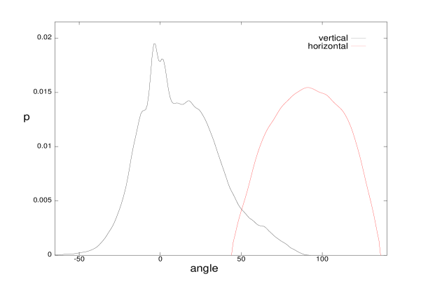
Figure 2: Distribution of vertical and horizontal angles (degrees)

3 Learning the Value of a Batted Ball

3.1 Bayesian Foundation

Given a set of observed batted balls and their outcomes, we will develop a method for learning the dependence of a batted ball’s value on its measured parameters. Let $x_{i}=(s_{i},v_{i},h_{i})$ for $i=1,2,\dots,n$ be a set of $n$ observed batted ball vectors where each vector has an associated outcome such as a single, a double, or an out. Using Bayes theorem, the probability of an outcome $R_{j}$ given a measured vector $x=(s,v,h)$ is given by

$$P(R_{j}|x)={{p(x|R_{j})P(R_{j})}\over{p(x)}}$$ (1)

where $p(x|R_{j})$ is the conditional probability density function for $x$ given outcome $R_{j},$ $P(R_{j})$ is the prior probability of outcome $R_{j},$ and $p(x)$ is the probability density function for $x.$ Linear combinations of the $P(R_{j}|x)$ probabilities for different outcomes can be used to model the expected value of statistics such as batting average, wOBA, and slugging percentage as a function of the batted ball vector $x.$ For a given batted ball, therefore, these statistics provide a measure of value that is separate from the batted ball’s particular outcome.

3.2 Kernel Density Estimation

The goal of density estimation for our application is to recover the underlying probability density functions $p(x|R_{j})$ and $p(x)$ in equation (1) from the set of observed batted ball vectors $x_{i}=(s_{i},v_{i},h_{i})$ and their outcomes. Given the typical positioning of defenders on a baseball field and the various ways that an outcome such as a single can occur, we expect a conditional density $p(x|R_{j})$ to have a complicated multimodal structure. Thus, we use a nonparametric technique for density estimation.

We first consider the task of estimating $p(x)$ from the $n$ batted ball vectors $x_{i}.$ Kernel methods [32] which are also known as Parzen-Rosenblatt [30] [31] window methods are widely used for nonparametric density estimation. A kernel density estimate for $p(x)$ is given by

$$\widehat{p}(x)={{1}\over{n}}\sum_{i=1}^{n}K(x-x_{i})$$ (2)

where $K(\cdot)$ is a kernel probability density function that is typically unimodal and centered at zero. A standard kernel for approximating a $d-$dimensional density is the zero-mean Gaussian

$$K(x)={{1}\over{(2\pi)^{d/2}|\Sigma|^{1/2}}}\exp\left[{-{{1}\over{2}}x^{T}\Sigma^{-1}x}\right]$$ (3)

where $\Sigma$ is the $d\times d$ covariance matrix. For this kernel, $\widehat{p}(x)$ at any $x$ is the average of a sum of Gaussians centered at the sample points $x_{i}$ and the covariance matrix $\Sigma$ determines the amount and orientation of the smoothing. $\Sigma$ is often chosen to be the product of a scalar and an identity matrix which results in equal smoothing in every direction. However, we see from figures 1 and 2 that the distribution for $v$ has detailed structure while the distributions for $s$ and $h$ are significantly smoother. Thus, to recover an accurate approximation $\widehat{p}(x)$ the covariance matrix should allow different amounts of smoothing in different directions. We enable this goal while also reducing the number of unknown parameters by adopting a diagonal model for $\Sigma$ with variance elements $(\sigma_{s}^{2},\sigma_{v}^{2},\sigma_{h}^{2}).$ For our three-dimensional data, this allows $K(x)$ to be written as a product of three one-dimensional Gaussians

$$K(x)={{1}\over{(2\pi)^{3/2}\sigma_{s}\sigma_{v}\sigma_{h}}}\exp\left[{-{{1}\over{2}}}\left({{s^{2}}\over{\sigma_{s}^{2}}}+{{v^{2}}\over{\sigma_{v}^{2}}}+{{h^{2}}\over{\sigma_{h}^{2}}}\right)\right]$$ (4)

which depends on the three unknown bandwidth parameters $\sigma_{s},\sigma_{v},$ and $\sigma_{h}.$

3.3 Bandwidth Selection

The accuracy of the kernel density estimate $\widehat{p}(x)$ is highly dependent on the choice of the bandwidth vector $\sigma=(\sigma_{s},\sigma_{v},\sigma_{h})$ [11]. The recovered $\widehat{p}(x)$ will be spiky for small values of the parameters and, in the limit, will tend to a sum of Dirac delta functions centered at the $x_{i}$ data points as the bandwidths approach zero. Large bandwidths, on the other hand, can induce excessive smoothing which causes the loss of important structure in the estimate of $p(x).$ A number of bandwidth selection techniques have been proposed and a recent survey of methods and software is given in [20]. Many of these techniques are based on maximum likelihood estimates for $p(x)$ which select $\sigma$ so that $\widehat{p}(x)$ maximizes the likelihood of the observed $x_{i}$ data samples. Applying these techniques to the full set of observed data, however, yields a maximum at $\sigma=(0,0,0)$ which corresponds to the sum of delta functions result. To avoid this difficulty, maximum likelihood methods for bandwidth selection have been developed that are based on leave-one-out cross-validation [32].

The computational demands of leave-one-out cross-validation techniques are excessive for our HITf/x data set. Therefore, we have adopted a cross-validation method which requires less computation. From the full set of $n$ observed $x_{i}$ vectors, we generate $M$ disjoint subsets $S_{j}$ of fixed size $n_{v}$ to be used for validation. For each validation set $S_{j},$ we construct the estimate $\widehat{p}(x)$ using the $n-n_{v}$ vectors that are not in $S_{j}$ as a function of the bandwidth vector $\sigma=(\sigma_{s},\sigma_{v},\sigma_{h}).$ The optimal bandwidth vector $\sigma_{j}^{*}=(\sigma_{sj}^{*},\sigma_{vj}^{*},\sigma_{hj}^{*})$ for $S_{j}$ is the choice that maximizes the pseudolikelihood [12] [20] according to

$$\sigma_{j}^{*}=\arg\max_{{}_{\vspace{1cm}{\textstyle\sigma}}}\prod_{x_{i}\in S_{j}}\widehat{p}(x_{i})$$ (5)

where the product is over the $n_{v}$ vectors in the validation set $S_{j}.$ The overall optimized bandwidth vector $\sigma^{*}$ is obtained by averaging the $M$ vectors $\sigma_{j}^{*}.$ We will present specific details of our implementation of this cross-validation method in section 4.2.

3.4 Constructing the Estimate for $P(R_{j}|x)$

An estimate for $P(R_{j}|x)$ can be derived from estimates of the quantities on the right side of equation (1). The density estimate $\widehat{p}(x)$ for $p(x)$ is obtained using the kernel method defined by equations (2) and (4) with the optimized bandwidth vector $\sigma^{*}$ learned using the process described in section 3.3. Each conditional probability density function $p(x|R_{j})$ is estimated in the same way except that the training set is defined by the subset of the $x_{i}$ vectors with outcome $R_{j}.$ Since reduced sample sizes for specific outcomes $R_{j}$ preclude the learning of individual bandwidth vectors for each $p(x|R_{j}),$ we use the $\sigma^{*}$ derived for $p(x)$ for each case. This approach also has the desirable effect of providing the same smoothing to a batted ball vector in the numerator and denominator of (1) which prevents a probability $P(R_{j}|x)$ from exceeding one. Each prior probability $P(R_{j})$ is estimated by the fraction of the $n$ batted balls in the full training set with outcome $R_{j}.$ The estimate for $P(R_{j}|x)$ is then constructed by combining the estimates for $p(x|R_{j}),P(R_{j}),$ and $p(x)$ according to Bayes theorem.

3.5 Intrinsic Value using wOBA

Our goal is to combine the posterior probabilities $P(R_{j}|x)$ into a measure of the intrinsic value of a batted ball as a function of $x.$ If we ignore bunts and treat sacrifice flies as ordinary outs, then the expected value of the traditional baseball statistics batting average and slugging percentage for a batted ball with parameter vector $x$ can be obtained from a linear combination of the $P(R_{j}|x)$ probabilities. These statistics, however, are deficient for describing the value of a batted ball. Batting average, for example, gives a home run and a single the same value while slugging percentage overvalues a home run at four times the value of a single. In 2007, Tango and his collaborators [36] defined wOBA as a linear combination of the probabilities of events in a baseball game. The wOBA coefficients that define the linear combination are derived from the average run value of each event. The original wOBA formulation includes events such as strikeouts and walks, but for our purposes we restrict the analysis to batted balls. The resulting formula is

$${\rm wOBA}(x)=\sum_{j=0}^{5}w_{j}P(R_{j}|x)$$ (6)

where the $w_{j}$ are the coefficients for the six batted ball outcomes $R_{0}=$ out, $R_{1}=$ single, $R_{2}=$ double, $R_{3}=$ triple, $R_{4}=$ home run, and $R_{5}=$ batter reaches on error.

4 Data Analysis

4.1 Batted Ball Data and wOBA Coefficients

The HITf/x data used for this study was provided by SportVision and includes measurements from every regular-season MLB game during 2014. The data set used for estimating wOBA$(x)$ consists of all balls in play with a horizontal angle in fair territory $(h\in[45^{\circ},135^{\circ}])$ that were tracked by the system where bunts are excluded. This results in a set of $n=124364$ batted balls which represents more than ninety-seven percent of the MLB total for 2014. The weights $w_{j}$ in equation (6) depend on the run environment and can change from year-to-year. Thus, for this 2014 batted ball data we use the coefficients $w_{0}=0.000,w_{1}=0.892,w_{2}=1.283,w_{3}=1.635,w_{4}=2.135,$ and $w_{5}=0.920$ where $w_{0},w_{1},w_{2},w_{3},$ and $w_{4}$ for 2014 were obtained from [40] and $w_{5}$ was obtained from [36]. In the following subsections we present details of the algorithm described in section 3 for learning wOBA$(x)$ from this data .

4.2 Cross-Validation for Density Estimation

The Bayesian method described in section 3.1 uses probability density estimates to compute the posterior probabilities $P(R_{j}|x).$ We use the model described in section 3.2 with the cross-validation method described in section 3.3 to estimate the densities. Five validation sets $S_{1},S_{2},S_{3},S_{4},$ and $S_{5}$ were used to select the optimized bandwidth vector $\sigma^{*}$ for the $p(x)$ estimate. Set $S_{i}$ includes $n_{v}$ batted balls that were hit on day $6i-5$ of a calendar month. Set $S_{2}$, for example, includes only batted balls hit on the 7th day of a month. The size $n_{v}=3820$ was taken to be the largest value so that each set $S_{i}$ includes the same number of elements. The decision to use six days of separation for the validation sets was made with the goal of maximizing the independence of the sets. A regular-season series of consecutive games between the same pair of teams always lasts less than six days. In addition, major league teams in 2014 tended to use a rotation of starting pitchers that repeats every five days so that, if this tendency is followed, each starting pitcher will occur once per calendar month in each of the five validation sets.

For each validation set $S_{j},$ a three-dimensional search was conducted with a step size of 0.1 in $\sigma_{s},\sigma_{v},$ and $\sigma_{h}$ to find the optimized $\sigma_{j}^{*}$ in equation (5). For each $S_{j}$ and $\sigma$ vector under consideration, we removed the twenty $x_{i}$ batted ball vectors with the smallest value of $\widehat{p}(x_{i})$ to prevent outliers from influencing the optimization. The vectors $\sigma_{j}^{*}$ for each $S_{j}$ are given in Table I and after averaging yielded an optimized $\sigma^{*}=(\sigma_{s}^{*},\sigma_{v}^{*},\sigma_{h}^{*})$ of $(2.02,1.50,2.20).$ We see that vertical angle has the smallest smoothing parameter $(\sigma_{v}^{*}=1.50)$ which is consistent with the observation from figures 1 and 2 that vertical angle has more detailed structure in its density than batted ball speed or horizontal angle.

TABLE I: Optimal bandwidths $\sigma_{j}^{*}$ for validation sets $S_{j}$

$S_{1}$	$S_{2}$	$S_{3}$	$S_{4}$	$S_{5}$
(2.0,1.5,2.2)	(1.9,1.5,2.3)	(2.0,1.6,2.0)	(2.0,1.6,2.3)	(2.2,1.3,2.2)

4.3 Visualizing the wOBA$(x)$ Function

We constructed the function wOBA$(x)$ for 2014 HITf/x data using the methods described in the previous sections. Figure 3 displays wOBA$(x)$ on the plane corresponding to a fixed initial speed $s$ of ninety-three miles per hour. For this value of $s,$ the best results for batters occur for balls hit with vertical angles between twenty-five and forty degrees that are near the right field foul line $(h\in[45^{\circ},55^{\circ}])$ or the left field foul line $(h\in[125^{\circ},135^{\circ}])$ where ballpark dimensions are typically the shortest. These batted balls often result in home runs. Batted balls hit at the same speed with the same vertical angle are less valuable at horizontal angles near ninety degrees which correspond to larger ballpark dimensions in center field. For this initial speed, batted balls with vertical angles near twelve degrees tend to carry over the infielders and land in front of the outfielders and have a high value for all horizontal angles. Typical horizontal angle positions for the three outfielders are evident from the three cold zones for balls hit in the air with $(v\in[15^{\circ},20^{\circ}])$ and typical horizontal positions for the four infielders are evident from the four cold zones for ground balls ($v<0).$

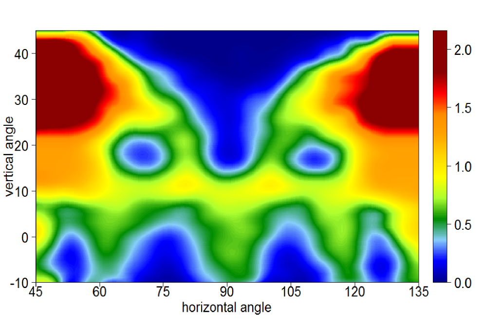
Figure 3: wOBA for an initial speed of 93 mph

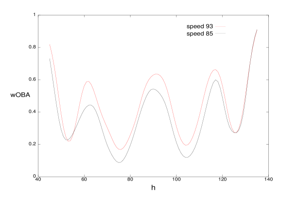
Figure 4: wOBA for a vertical angle $v$ of $-2^{\circ}$

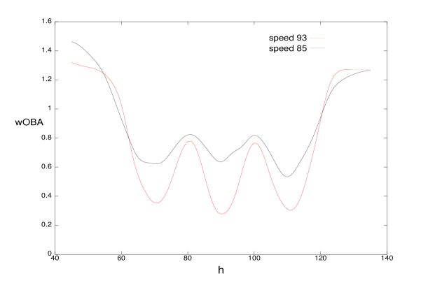
Figure 5: wOBA for a vertical angle $v$ of $+15^{\circ}$

Figures 4 and 5 examine properties of the wOBA$(x)$ function in more detail. Figure 4 plots wOBA as a function of the horizontal angle $h$ for $s=85$ mph and $s=93$ mph with the vertical angle fixed at $v=-2^{\circ}$. Since this negative value of $v$ corresponds to ground balls, minima in the two curves correspond to the typical position of infielders with the minima near $53^{\circ},76^{\circ},104^{\circ},$ and $126^{\circ}$ corresponding to the first baseman, second baseman, shortstop, and third baseman respectively. Over most horizontal angles, balls hit at 93 mph have a higher value than balls hit at 85 mph since ground balls hit at a higher speed have a higher probability of eluding a defender. Figure 5 plots wOBA as a function of the horizontal angle $h$ for $s=85$ and $s=93$ with the vertical angle fixed at $v=+15^{\circ}$. Since this positive value of $v$ corresponds to balls hit in the air, minima in the two curves correspond to the typical position of outfielders with the minima near $70^{\circ},90^{\circ},$ and $110^{\circ}$ corresponding to the right fielder, center fielder, and left fielder respectively. For this vertical angle, balls hit in the direction of an outfielder have a higher value for a speed of 85 mph because these balls often fall in front of the outfielder for hits while balls hit at 93 mph more frequently carry to the outfielder for outs. In both figures, the largest wOBA values occur for balls hit near the foul lines ($h=45^{\circ}$ or $h=135^{\circ}$) which often result in extra-base hits instead of singles.

4.4 Dependence of wOBA$(x)$ on Batter Handedness

Significant wOBA$(x)$ differences between left-handed and right-handed batters occur due to differences in the positioning of defenders. Thus, we repeated the process described in the previous sections to obtain wOBA$l(x)$ for left-handed batters and wOBA$r(x)$ for right-handed batters. The $n=124364$ batted balls described in section 4.1 were first partitioned into the 54948 for left-handed batters and 69416 for right-handed batters. The method described in section 4.2 was then used to build five validation sets for each case which resulted in a validation set size $n_{v}$ of 1680 for wOBA$l(x)$ and 2190 for wOBA$r(x).$ The optimal bandwidth vectors $\sigma_{j}^{*}$ for each validation set and batter handedness are given in Table II. After averaging, we arrive at an optimized $\sigma^{*}=(\sigma_{s}^{*},\sigma_{v}^{*},\sigma_{h}^{*})$ of $(2.18,1.72,2.50)$ for wOBA$l(x)$ and $(2.16,1.56,2.30)$ for wOBA$r(x).$ We note that, as seen in section 4.2, $\sigma_{v}^{*}$ is the smallest for each case while $\sigma_{h}^{*}$ is the largest. In addition, the bandwidth increases for each variable to provide more smoothing as the number of samples decreases.

TABLE II: Optimal bandwidths $\sigma_{j}^{*}$ for validation sets $S_{j}$ by batter handedness

	$S_{1}$	$S_{2}$	$S_{3}$	$S_{4}$	$S_{5}$
L	(2.0,1.5,3.1)	(2.2,2.1,2.2)	(2.3,1.6,2.1)	(2.4,1.9,2.3)	(2.0,1.5,2.8)
R	(1.9,1.8,2.1)	(2.1,1.7,2.2)	(2.4,1.4,2.2)	(2.2,1.5,2.6)	(2.2,1.4,2.4)

Figures 6 and 7 examine differences between wOBA$l(x)$ and wOBA$r(x).$ These figures consider specifically batted balls hit at 93 miles per hour at the vertical angles shown in figure 4 and figure 5. Figure 6 considers ground balls hit with a vertical angle of $-2^{\circ}.$ As in figure 4, we observe four minima in each curve that correspond to the typical position of the four infielders. We see, however, that the minima for left-handed batters are shifted several degrees toward the first base line $(h=45^{\circ})$ compared to the corresponding minima for right-handed batters. This shift corresponds to the difference in fielder positioning as a function of batter handedness. We also see that ground balls near the first base line $(h=45^{\circ})$ have a higher value for right-handed batters since there is a lower probability of a defender in that region and that ground balls near the third base line $(h=135^{\circ})$ have a higher value for left-handed batters. Figure 7 examines the impact of batter handedness on balls hit at 93 miles per hour with a vertical angle of $+15^{\circ}.$ The three minima in each curve correspond to the typical positions of outfielders. We see that the minima are shifted several degrees toward the right field line $(h=45^{\circ})$ for left-handed batters. We also see that left-handed batters have an advantage for batted balls hit in the direction of the right fielder ($h\approx 70^{\circ}$) since the right fielder is typically playing deeper for left-handed batters which allows additional batted balls to fall safely for hits. We observe the opposite effect for batted balls hit in the direction of the left fielder ($h\approx 110^{\circ}$) since the left fielder is typically playing deeper for right handed batters.

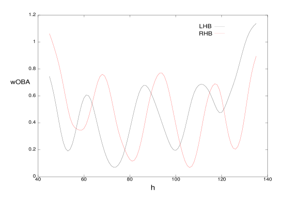
Figure 6: wOBA for speed 93 mph and vertical angle $-2^{\circ}$

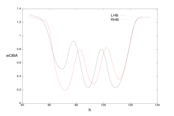
Figure 7: wOBA for speed 93 mph and vertical angle $+15^{\circ}$

5 Exploiting the Model

5.1 Intrinsic Value versus Observed Outcome

Using the model developed in sections 3 and 4, a batted ball $b$ with parameter vector $x$ can be assigned the intrinsic value $I(b)$ given by either wOBA$l(x)$ or wOBA$r(x)$ depending on the handedness of the batter. Batted balls may also be assigned an observed value $O(b)$ given by the wOBA coefficient for the result of the batted ball so that, for example, $O(b)=1.283$ for a batted ball that results in a double. The observed value $O(b)$ depends on several factors that are beyond the control of the batter and the pitcher such as the defense, the weather, and the ballpark. In early May 2014, for example, batter Evan Longoria hit a high fly ball with an $I(b)$ of $0.040$ that is usually an easy out, but the center fielder lost the ball in the lights and the result was a triple with an $O(b)$ of 1.635. In this section, we describe several statistics that can be generated using the intrinsic $I(b)$ value for a batted ball.

5.2 Intrinsic Contact Measure for Batters

Analysts sometimes attempt to quantify the value of a hitter’s batted balls using the average $\overline{O}$ of his observed $O(b)$ over a period of time. This statistic $\overline{O}$ is referred to as wOBA on contact or wOBAcon [23]. As we pointed out in section 5.1, however, $\overline{O}$ depends on a number of variables that are independent of the batter’s quality of contact. Thus, we propose the average $\overline{I}$ of the intrinsic values $I(b)$ as a more accurate valuation of a hitter’s collection of batted balls. Table III presents the batters with the highest $\overline{I}$ in 2014 among players who hit at least 300 batted balls that were tracked by HITf/x. These players are known for their ability to generate hard-hit balls.

TABLE III: Batters with the highest $\overline{I}$ in 2014 over at least 300 batted balls

Batter	$\overline{I}$
Giancarlo Stanton	0.526
Mike Trout	0.498
Miguel Cabrera	0.488
J.D. Martinez	0.482
Matt Kemp	0.477
Brandon Moss	0.476
Jose Abreu	0.469
Michael Morse	0.468
Corey Dickerson	0.465
Edwin Encarnacion	0.461

For an individual batter, several factors can contribute to differences between the average observed outcome $\overline{O}$ and the intrinsic value $\overline{I}$ of his batted balls. Batters who are fast runners, for example, force infielders to play shallower which compromises range and leads to additional hits. Fast runners also tend to beat out more infield hits and garner additional bases on hits to the outfield. Thus, a faster runner will tend to achieve a higher $\overline{O}$ for a given $\overline{I}.$ Batters with a high degree of predictability in their batted balls, such as left-handed batters who hit a large majority of their ground balls to the right of second base, are easier to defend than batters who produce a more uniform distribution of batted balls. Batters with a higher degree of predictability, therefore, will tend to have a lower $\overline{O}$ for a given $\overline{I}.$ Random noise, which is often referred to as luck in this context, can also play a role in creating differences between $\overline{O}$ and $\overline{I}.$ Thus, our model for $\overline{I}$ is a useful starting point for separating the contribution of factors such as intrinsic contact ability, running speed, batted ball distribution, and luck on the observed $\overline{O}.$ Since noise contributions will tend to be independent from year-to-year and the other factors will be represented by statistics with different reliabilities and aging curves, the ability to separate these factors has value for projection systems.

Table IV presents batters with the largest values of $\overline{O}-\overline{I}$ during the 2014 season where both $\overline{O}$ and $\overline{I}$ are computed using the batted balls tracked by HITf/x. Most of the players in the table have above average running speed with Hamilton and Cain having exceptional speed. The top two players on the list also benefited from good luck. Starling Marte led major league baseball by reaching base on an error fourteen times in 2014 which contributed to his MLB leading $\overline{O}-\overline{I}.$ Jose Abreu also experienced significant good fortune as many of his 36 home runs just barely cleared the fence causing his home runs to have an average intrinsic value $I(b)$ of 1.461 which is significantly less than the corresponding $O(b)$ of 2.135. Abreu’s $\overline{O}-\overline{I}$ difference on home runs explains nearly all of his total $\overline{O}-\overline{I}$ difference in the table and his luck on home runs even attracted the attention of the mainstream media during the 2014 season [3].

TABLE IV: Batters with the highest $\overline{O}-\overline{I}$ in 2014 over at least 300 batted balls

Batter	$\overline{O}-\overline{I}$
Starling Marte	0.072
Jose Abreu	0.063
Yasiel Puig	0.060
Adam Eaton	0.060
Billy Hamilton	0.060
Lorenzo Cain	0.059
J.D. Martinez	0.053
Josh Harrison	0.052
Andrew McCutchen	0.051
Hunter Pence	0.049

Table V presents batters with the lowest values of $\overline{O}-\overline{I}$ during the 2014 season using the batted balls tracked by HITf/x. All of the batters in this table have below average running speed and several (Moss, Teixeira, Santana) also had sufficiently predictable batted ball distributions that opposing teams were able to employ extreme defensive shifts. These factors contributed to the small $\overline{O}-\overline{I}$ values shown in Table V.

TABLE V: Batters with the Lowest $\overline{O}-\overline{I}$ in 2014 over at least 300 batted balls

Batter	$\overline{O}-\overline{I}$
Billy Butler	-0.055
Brandon Moss	-0.043
Yadier Molina	-0.042
Miguel Cabrera	-0.042
Matt Dominguez	-0.041
Alberto Callaspo	-0.039
Mark Teixeira	-0.038
Albert Pujols	-0.038
Carlos Santana	-0.036
Buster Posey	-0.032

5.3 Intrinsic Opponent Contact Measure for Pitchers

In 2001, McCracken [26] suggested that pitchers have little control over the result of opponent batted balls that are not home runs. Since then, however, a number of researchers [5] [15] [16] [24] [34] [35] [37] have presented evidence that pitchers can affect the expected outcome of balls in play. Despite this progress, however, models that isolate the impact of the pitcher on the fate of batted balls have been elusive due to the confounding effects of the defense, ballpark, weather, and luck on a batted ball’s outcome. Since the HITf/x system characterizes a batted ball at contact, the influence of these confounding factors can be removed. As proposed in section 5.2 for batters, we can assign the intrinsic value $\overline{I}$ to the collection of batted balls allowed by a pitcher. The statistic $\overline{I}$ provides a context-invariant measure of a pitcher’s opponent contact which allows this aspect of his performance to be accurately quantified.

Table VI presents the pitchers with the lowest $\overline{I}$ values in 2014 among those who allowed at least 300 batted balls that were tracked by HITf/x. Eight of the ten pitchers in the table had an average fastball speed in 2014 that was above the league average and Garrett Richards, who earned the top spot in Table VI, enjoyed one of the highest average fastball speeds in MLB. The success of the two softer tossing pitchers on the list was due in part to an exceptional sinker for Dallas Keuchel and an exceptional split-finger fastball for Alex Cobb. An interesting topic for future research will be to study pitcher characteristics that lead to low values of $\overline{I}.$

TABLE VI: Pitchers with the lowest opponent $\overline{I}$ over at least 300 batted balls, 2014

Pitcher	$\overline{I}$
Garrett Richards	0.304
Anibal Sanchez	0.309
Danny Duffy	0.314
Chris Sale	0.319
Matt Garza	0.328
Dallas Keuchel	0.329
Jarred Cosart	0.329
Clayton Kershaw	0.332
Alex Cobb	0.336
Johnny Cueto	0.337

5.4 Defense and Environmental Effects

5.4.1 Contact-Adjusted Defense

Many statistics have been designed to measure team defense. Defensive efficiency ratio (DER) [21], for example, measures the fraction of the time that a team’s defense records an out on a batted ball that is not a home run. While DER is a useful measure of defense that is easy to compute, the statistic does not account for the difficulty of fielding a batted ball or distinguish between different results such as a single or a double. These deficiencies have led to the development of the advanced fielding metrics defensive runs saved (DRS) [10] and ultimate zone rating (UZR) [25]. These metrics use data from Baseball Info Solutions (BIS) that partition batted balls into types such as bunts, ground balls, line drives, and fly balls and the speed categories of soft, medium, and hard. In addition, the DRS system uses video scouts and timer data to further partition batted balls into speed bins that have a width of 10 mph so that, for example, batted balls hit between 65 and 75 mph are sorted into the same bin. DRS and UZR generate measures of player and team defense in units of runs above average.

The use of HITf/x data has the potential to improve on the accuracy of defensive metrics by exploiting higher resolution measurements of batted ball speed and direction than are available with BIS data. Using the difference between the intrinsic $I(b)$ and observed $O(b)$ value of a batted ball as defined in section 5.1, we obtain a simple automated technique for measuring contact-adjusted team defense that can serve as the basis for a HITf/x-based defensive metric. For this application, we build the underlying wOBA$l(x)$ and wOBA$r(x)$ models using the subset of batted balls that are not home runs. For the 2014 HITf/x data this results in 120231 batted balls. Each team’s contact-adjusted defense is defined as $D=\overline{I}-\overline{O}$ where the averages $\overline{I}$ and $\overline{O}$ are computed over the batted balls tracked by HITf/x that are not home runs while the team is in the field. Thus $D$ will be positive for teams that are above average and negative for teams that are below average. Table VII presents the teams with the top five and the bottom five values of $D$ among the 30 major league teams in 2014. We also include each team’s corresponding rank according to the DRS and UZR systems. We note that DRS and UZR include a number of additional factors which are not included in $D$ such as bunt defense, the quality of outfield throwing arms, and the ability of infielders to turn double plays. Nevertheless, we see that the best defensive teams according to $D$ tend to have high ratings according to DRS and UZR and that the worst defensive teams according to $D$ tend to have low ratings according to DRS and UZR. We note that Seattle receives a significantly more favorable rating using $D$ relative to the other systems but this this can be explained by environmental factors that will be discussed in section 5.4.2.

TABLE VII: Teams with the highest and lowest Contact-Adjusted Defense $D,$ 2014

Team	$D$	$D$ Rank	DRS Rank	UZR Rank
Oakland Athletics	0.018	1	7	8
Baltimore Orioles	0.013	2	3	2
Seattle Mariners	0.011	3	19	10
Cincinnati Reds	0.010	4	1	4
San Diego Padres	0.009	5	5	9
Toronto Blue Jays	-0.013	26	23	21
Chicago White Sox	-0.017	27	27	26
Detroit Tigers	-0.018	28	28	28
Minnesota Twins	-0.018	29	29	25
Cleveland Indians	-0.018	30	30	30

5.4.2 Environmental Effects

We can examine the impact of the environment on batted balls by comparing a team’s contact-adjusted defense for home and away games. For each team we define the difference

$$D_{HA}=D_{H}-D_{A}$$ (7)

where $D_{H}$ denotes $D$ for the team in home games and $D_{A}$ denotes $D$ for the team in away games. Thus, large positive values of $D_{HA}$ suggest that a team’s home ballpark benefits the defense while negative values suggest an environment that is less favorable for defenders. Several factors can contribute to a team’s observed $D_{HA}.$ For a batted ball hit with a given parameter vector $x$ at contact, for example, the ambient wind and air density will have a significant effect on the speed of the ball as it travels which affects the ability of defenders to make a play [1][28]. In addition, ballparks with slower infields or smaller outfield areas will tend to be easier to defend. Locations with high outfield walls lead to smaller values of $D$ due to uncatchable balls that hit high on a wall but which are either easy outs or home runs in other parks. We note that the DRS and UZR systems make adjustments for several of these environmental factors.

Table VIII presents the major league teams with the five highest and five lowest values of $D_{HA}$ during 2014. We see that the environmental effects can be quite substantial especially for teams with positive values of $D_{HA}.$ San Diego and Seattle have the largest values of $D_{HA}$ which is consistent with observations of high air density in these locations. In addition, Seattle, Philadelphia, Milwaukee, and Baltimore play in home parks with smaller than average areas in the outfield [18] which contributes to high values of $D_{HA}.$ There is also evidence that Philadelphia, Milwaukee, and Baltimore had home parks with slow infields in 2014. For games involving the Orioles in 2014, there was a twenty-eight point higher batting average on ground balls in road games than in home games and the corresponding differences were fifteen points for Milwaukee and ten points for Philadelphia. Among teams with the smallest $D_{HA},$ Boston and Minnesota have home ballparks with high walls that lead to uncatchable balls in play. The Rockies, Angels, and Mets play in home ballparks with above average outfield areas which makes batted balls more difficult to defend in these locations. In particular, the Rockies have the ballpark with the largest outfield area while the Mets stadium is the third largest. In addition, games in Colorado are characterized by a low air density [28] which also tends to make defense more difficult.

TABLE VIII: Teams with the highest and lowest $D_{HA}$ in 2014

Team	$D_{HA}$	Rank
San Diego Padres	0.043	1
Seattle Mariners	0.031	2
Philadelphia Phillies	0.026	3
Milwaukee Brewers	0.024	4
Baltimore Orioles	0.021	5
New York Mets	-0.006	26
Los Angeles Angels	-0.009	27
Colorado Rockies	-0.014	28
Minnesota Twins	-0.017	29
Boston Red Sox	-0.018	30

6 Conclusion

The amount of sensor data that is available to support sports analytics is rapidly increasing [4] [17] [22] [39]. This data has created unprecedented opportunities to exploit machine learning techniques to model players and strategies [27] [38] [41]. In this work we have used HITf/x sensor data for more than one hundred thousand batted balls hit during the 2014 MLB season to learn a model for a batted ball’s intrinsic value which is invariant to contextual factors that can impact its outcome. The model is constructed using a Bayesian framework that includes kernel density estimates that are learned using cross-validation. The intrinsic measure for contact quality is derived from the wOBA linear weights model for run value. The new approach successfully separates factors that are under the control of the batter and pitcher from contextual factors that are characteristic of the environment.

We have used the model developed in this paper to define statistics that measure the intrinsic quality of contact for batters and pitchers. These statistics are influenced less by random variation from contextual variables than traditional statistics that depend on batted ball outcomes. In addition, the new statistics can be used to separate the various skill components that contribute to a player’s performance on batted balls. A batter’s performance, for example, can be partitioned into statistics that measure his intrinsic contact, running speed, and batted ball distribution which determines susceptibility to defensive shifts. A pitcher’s performance can be divided into statistics that measure his opponent intrinsic contact and fielding ability. An important advantage of generating separate statistics to represent distinct skills is that each statistic can be regressed and projected using its individual reliability and aging curve during forecasting. The new statistics also allow us to investigate how players control quality of contact. In section 5.3, for example, we observed that many of the pitchers who were the most effective at controlling contact also exhibited an above-average fastball velocity. Given the wealth of descriptors measured by the PITCHf/x system [17], we have the opportunity to characterize the relationship between the quality of a pitcher’s opponent contact and his distribution and sequencing of pitches. Similarly, we can study the relationship between a batter’s intrinsic contact and his swing parameters [29].

We have also examined the role of contextual factors that are beyond the control of the batter and pitcher on the result of a batted ball. In section 5.4.1 we used the intrinsic contact model developed in this paper to derive a simple automated measure of contact-adjusted defense. We showed that this measure is reasonably consistent with advanced defensive metrics and that there are significant differences in defensive capability across teams. In section 5.4.2 we showed that environmental factors such as ballpark dimensions and weather conditions also have a significant effect on the outcome of a batted ball. Given the granularity of HITf/x data and the capability of density estimation techniques, the methods used in this paper could be adopted to design defensive metrics and ballpark models that are a function of the batted ball vector $x=(s,v,h).$ This would allow a player’s collection of batted balls to be translated to a new environment. A forecasting system equipped with these models could accurately predict, for example, how a given batter might perform in a new ballpark or how a given pitcher might benefit from an improved infield defense.

Glenn Healey is Professor of Electrical Engineering and Computer Science at the University of California, Irvine. Before joining UC Irvine, he worked at IBM Research. Dr. Healey received the B.S.E. degree in Computer Engineering from the University of Michigan and the M.S. degree in computer science, the M.S. degree in mathematics, and the Ph.D. degree in computer science from Stanford University. He is director of the Computer Vision Laboratory at UC Irvine. Dr. Healey has served on the editorial boards of IEEE Transactions on Pattern Analysis and Machine Intelligence, IEEE Transactions on Image Processing, and the Journal of the Optical Society of America A. He has been elected a Fellow of IEEE and SPIE. Dr. Healey has received several awards for outstanding teaching and research.

References

- [1] R. Adair. The Physics of Baseball. Perennial, New York, 3rd edition, 2002.
- [2] B. Baumer and A. Zimbalist. The Sabermetric Revolution: Assessing the growth of analytics in baseball. University of Pennsylvania Press, Philadelphia, 2014.
- [3] A. Beaton. (July 27, 2014). Jose Abreu: the champion of the cheap home run [Online]. Available: www.wsj.com/articles/jose-abreu-the-champion-of-the-cheap-home-run-1406514931.
- [4] B. Bowman and J. Inzerillo. MLBAM: putting the D in data. In Sloan Sports Analytics Conference, Boston, 2014.
- [5] J.C. Bradbury. (May 24, 2005). Another look at DIPS [Online]. Available: www.hardballtimes.com/another-look-at-dips1.
- [6] J.C. Bradbury. Peak athletic performance and ageing: evidence from baseball. Journal of Sports Sciences, 27(6):599–610, 2009.
- [7] R. Carleton. (Jul. 16, 2012). It’s a small sample size after all [Online]. Available: www.baseball.prospectus.com/ article.php?articleid=17659.
- [8] R. Carleton. (May 9, 2013). Should I worry about my favorite pitcher? [Online]. Available: www.baseballprospectus. com/article.php?articleid=20516.
- [9] B. Cartwright. What ground balls can tell us about fly balls. In J. Distelheim, G. Simons, and C. Hale, editors, The Hardball Times Baseball Annual, 2012, pages 249–254. ACTA Sports, Chicago, 2011.
- [10] J. Dewan. Defensive runs saved [Online]. Available: fieldingbible.com/summary.asp.
- [11] R. Duda, P. Hart, and D. Stork. Pattern Classification. Wiley-Interscience, New York, 2001.
- [12] R. Duin. On the choice of smoothing parameters for Parzen estimators of probability density functions. IEEE Transactions on Computers, C-25(11):1175–1179, 1976.
- [13] G. DuPaul. (Jan. 4, 2013). Projecting BABIP and regression toward the mean [Online]. Available: www.beyondtheboxscore. com/2013/1/4/3827868/projecting-babip-regression-toward-the-mean-baseball-math-sabermetrics.
- [14] B. Efron and C. Morris. Stein’s paradox in statistics. Scientific American, 236(5):119–127, 1977.
- [15] M. Fast. (Nov. 16, 2011). Who controls how hard the ball is hit? [Online]. Available: www.baseballprospectus.com/article. php?articleid=15532.
- [16] M. Fast. (Nov. 22, 2011). How does quality of contact relate to BABIP? [Online]. Available: www.baseballprospectus. com/article.php?articleid=15562.
- [17] M. Fast. What the heck is PITCHf/x? In J. Distelheim, B. Tsao, J. Oshan, C. Bolado, and B. Jacobs, editors, The Hardball Times Baseball Annual, 2010, pages 153–158. The Hardball Times, 2010.
- [18] C. Gaines. (Mar. 26, 2014). MLB ballpark sizes show the immense difference between Fenway Park and Coors Field [Online]. Available: www.businessinsider.com/chart-major-league-baseball-ballpark-sizes-2014-3.
- [19] S. Goldman and C. Kahrl, editors. Baseball Prospectus 2008. Penguin Group, New York, 2008.
- [20] A.C. Guidoum. Kernel estimator and bandwidth selection for density and its derivatives. The kedd package, version 1.03, October 2015.
- [21] B. James. 1978 Baseball Abstract. Self-published, Lawrence, Kansas, 1978.
- [22] P. Jensen. (Jun. 30, 2009). Using HITf/x to measure skill [Online]. Available: www.hardballtimes.com/using-hitf-x-to-measure-skill.
- [23] J. Judge. (Aug. 13, 2014). Scapegoating the shift for the decline in offense [Online]. Available: www.hardballtimes.com/ scapegoating-the-shift-for-the-decline-in-offense.
- [24] M. Lichtman. (Feb. 29, 2004). DIPS revisited [Online]. Available: www.baseballthinkfactory.org/primate_studies/discussion/ lichtman_2004-02-29_0.
- [25] M. Lichtman. (May 19, 2010). The FanGraphs UZR primer [Online]. Available: www.fangraphs.com/blogs/the-fangraphs-uzr-primer.
- [26] V. McCracken. (Jan. 23, 2001). Pitching and defense: How much control do hurlers have? [Online]. Available: www.baseball-prospectus.com/article.php?articleid=878.
- [27] A. Miller, L. Bornn, R. Adams, and K. Goldsberry. Factorized point process intensities: A spatial analysis of professional basketball. In International Conference on Machine Learning, pages 235–243, 2014.
- [28] A. Nathan. Baseball at high altitude [Online]. Available: baseball.physics.illinois.edu/Denver.html.
- [29] A. Nathan. (Dec. 24, 2015). Optimizing the swing, part deux: Paying homage to Teddy Ballgame [Online]. Available: www.hardballtimes.com/optimizing-the-swing-part-deux-paying-homage-to-teddy-ballgame.
- [30] E. Parzen. On estimation of a probability density function and mode. Annals of Mathematical Statistics, 33(3):1065–1076, 1962.
- [31] M. Rosenblatt. Remarks on some nonparametric estimates of a density function. Annals of Mathematical Statistics, 27(3):832–837, 1956.
- [32] S. Sheather. Density estimation. Statistical Science, 19(4):588–597, 2004.
- [33] N. Silver. Why was Kevin Maas a bust? In J. Keri, editor, Baseball between the numbers, pages 253–271. Basic Books, New York, 2006.
- [34] M. Swartz. (Dec. 15, 2010). Ground-ballers: better than you think [Online]. Available: www.baseballprospectus.com/arti-cle.php?articleid=12581.
- [35] M. Swartz. (Mar. 17, 2010). Why SIERA doesn’t throw BABIP out with the bath water [Online]. Available: www.baseballprospectus. com/article.php?articleid=10281.
- [36] T. Tango, M. Lichtman, and A. Dolphin. The Book: Playing the Percentages in Baseball. Potomac Books, Dulles, Virgina, 2007.
- [37] T. Tippett. (Jul. 21, 2003). Can pitchers prevent hits on balls in play? [Online]. Available: 207.56.97.150/articles/ipavg2.htm.
- [38] X. Wei, P. Lucey, S. Morgan, P. Carr, M. Reid, and S. Sridharan. Predicting serves in tennis using style priors. In ACM SIGKDD International Conference on Knowledge Discovery and Data Mining, pages 2207–2215, Sydney, 2015.
- [39] M. Wilson. (June 20, 2012). Moneyball 2.0: How missile tracking cameras are remaking the NBA [Online]. Available: www.fastcodesign.com/1670059/moneyball-20-how-missile-tracking-cameras-are-remaking-the-nba.
- [40] wOBA and FIP constants [Online]. Available: www.fangraphs. com/guts.aspx?type=cn.
- [41] Y. Yue, P. Lucey, P. Carr, A. Bialkowski, and I. Matthews. Learning fine-grained spatial models for dynamic sports play prediction. In IEEE International Conference on Data Mining, 2014.