Low-mass Active Galactic Nuclei with Rapid X-ray Variability

Abstract

We present a detailed study of the optical spectroscopic properties of 12 active galactic nuclei (AGNs) with candidate low-mass black holes (BHs) selected by Kamizasa et al. through rapid X-ray variability. The high-quality, echellette Magellan spectra reveal broad H$\alpha$ emission in all the sources, allowing us to estimate robust viral BH masses and Eddington ratios for this unique sample. We confirm that the sample contains low-mass BHs accreting at high rates: the median $M_{\rm BH}=1.2\times 10^{6}$ $M_{\odot}$ and median $L_{\rm bol}/L_{\rm Edd}=0.44$. The sample follows the $M_{\rm BH}-\sigma_{*}$ relation, within the considerable scatter typical of pseudobulges, the probable hosts of these low-mass AGNs. Various lines of evidence suggest that ongoing star formation is prevalent in these systems. We propose a new strategy to estimate star formation rates in AGNs hosted by low-mass, low-metallicity galaxies, based on modification of an existing method using the strength of [O II] $\lambda$3727, [O III] $\lambda$5007, and X-rays.

1 Introduction

Central black holes (BHs) constitute an integral component of the nuclear regions of galaxies. Much progress has been made in the detection and characterization of the statistical properties of supermassive BHs in nearby galaxies, over the mass range $M_{\rm BH}$ $\approx 10^{6}-10^{10}$ $M_{\odot}$ (e.g., Gültekin et al. 2009; McConnell & Ma 2013; Kormendy & Ho 2013). During the last 10 years, there has also been a number of successful attempts to identify the rarer population of lower mass central BHs, with $M_{\rm BH}$ $\mathrel{\hbox{\hbox to0.0pt{\hbox{\lower 4.0pt\hbox{$\sim$}}\hss}\hbox{$<$}}}$ $10^{6}$ $M_{\odot}$, in bands ranging from the optical (e.g., Greene & Ho 2004, 2007c; Barth et al. 2008; Seth et al. 2010; Dong et al. 2012b; Reines et al. 2013; Moran et al. 2014; Baldassare et al. 2015), to the radio (Reines et al. 2011, 2014), and the mid-infrared (Satyapal et al. 2008, 2009, 2014; Goulding & Alexander 2009). X-ray images, particularly at high angular resolution, can effectively identify candidate active galactic nuclei (AGNs) as compact nuclear cores in low-mass, late-type—even dwarf—galaxies (Desroches & Ho 2009; Zhang et al. 2009; Reines et al. 2011, 2014; Araya Salvo et al. 2012; Schramm et al. 2013; Lemons et al. 2015).

Exploiting the fact that the amplitude of X-ray variability in AGNs scales inversely with BH mass (e.g., Lu & Yu 2001; Papadakis 2004; McHardy et al. 2006), Kamizasa et al. (2012) used the Second XMM-Newton Serendipitous Source Catalogue (Watson et al. 2009) to select a sample of 16 AGNs with candidate low-mass BHs, based on the presence of rapid variability in their X-ray light curve. For the 15 sources for which they could compute the “normalized excess variance” in the 0.5–10 keV band, they estimate that their sample contains $M_{\rm BH}$ $\approx(1.1-6.6)\times 10^{6}$ $M_{\odot}$. The subset with available redshift estimates has an inferred median Eddington ratio of $\lambda_{\rm E}\equiv L_{\rm bol}/L_{\rm Edd}=0.24$, where $L_{\rm bol}$ is the bolometric luminosity and $L_{\rm Edd}$ is the Eddington luminosity. The remaining object, 2XMM J123103.2+110648, has an exceptionally prominent soft X-ray excess, which Terashima et al. (2012) model with a multicolor disk blackbody with an inner disk temperature of $kT=0.16-0.21$ keV. In a follow-up optical study, Ho et al. (2012) confirm the AGN nature of the source but find that it emits only narrow emission lines, an unexpected result given the lack of significant intrinsic X-ray absorption and the high Eddington ratio ($\lambda_{\rm E}$ $\mathrel{\hbox{\hbox to0.0pt{\hbox{\lower 4.0pt\hbox{$\sim$}}\hss}\hbox{$>$}}}$ 0.5) derived from its estimated BH mass of $\sim 10^{5}$ $M_{\odot}$.

The majority of Kamizasa et al.’s sample has no previous optical spectroscopic data, not even basic information such as spectroscopic redshifts, making it impossible to derive many fundamental parameters for this unique sample. Moreover, in light of the intriguing properties of 2XMM J123103.2+110648, it would be of interest to investigate the optical spectral properties of these objects more systematically. This paper reports detailed high-resolution , high–signal-to-noise ratio (S/N) optical spectra for 12 of the 15 sources from the sample of Kamizasa et al. (2012) with BH masses previously estimated through X-ray variability. As the sample was initially designed to select low-mass objects, we anticipate the emission lines, both broad and narrow, to have small velocity widths; moderately high dispersion would be required to measure useful kinematics.

2 Observations, Data Reduction, and Spectral Fits

The observations, summarized in Table 1, were obtained with the Magellan 6.5m Clay telescope at Las Campanas Observatory, during the course of two observing runs in 2013, using the Magellan Echellette (MagE) spectrograph (Marshall et al. 2008). The spectra cover $\sim$3100 Å to 1 $\mu$m in 15 spectral orders at a resolving power for a 1^′′ slit, as determined from the sky emission lines, of $\lambda/\Delta\lambda=4627$, which corresponds to an instrumental velocity dispersion of $\sigma_{i}=27.6$ km s^-1. The brightnesses of the sources range from $g\approx 18$ to 21 mag. We observed featureless standard stars for flux calibration and telluric correction, as well as late-type stellar templates for velocity dispersion measurement. The observing conditions were mostly photometric, but the observations were occasionally carried out under thin cirrus. The seeing varied from 0$\farcs$6 to 1$\farcs$2.

The slit was aligned along the parallactic angle to minimize slit losses due to differential atmospheric refraction.

The data were reduced using the IDL routine mage_reduce developed and kindly provided by George Becker. We performed flat-fielding correction using twilight flats and contemporaneous dome flats taken just after each science exposure. Wavelength calibration was done using ThAr arc spectra. After extracting 1-D spectra, we apply flux calibration and telluric correction. We correct for Galactic extinction using the extinction values of Schlafly & Finkbeiner (2011) and the reddening curve of Cardelli et al. (1989).

Figure 1 shows the final spectra for the sample. Strong emission lines, and in some cases a featureless continuum, are present in all the sources, superposed on a weak stellar continuum characteristic of intermediate-age stars. The strong emission lines, particularly [O III] $\lambda$5007, allow us to determine— accurately and for the first time in most cases—the redshifts of the sample (Table 1). We decompose the spectra into host galaxy starlight, a featureless AGN power-law continuum, Fe II pseudocontinuum, and a residual, pure emission-line spectrum, closely following the treatment described in Ho & Kim (2009). We perform a multi-component Gaussian fit of the continuum-subtracted spectrum to derive fluxes, widths, and radial velocities of the major broad and narrow emission lines (see bottom panels of each object in Figure 1). To isolate the broad H$\alpha$ line, we follow previous practice (e.g., Ho et al. 1997) and constrain the profile of [N II] $\lambda$$\lambda$6548, 6583 and the narrow component of H$\alpha$ to that of [S II] $\lambda$$\lambda$6716, 6731. Likewise, we tie the narrow component of H$\beta$ to [O III] $\lambda$5007. Each of the lines of the [S II] doublet usually can be fit adequately with a single Gaussian, whereas [O III] requires an extended, often blueshifted, wing component in addition to a Gaussian core. The final,

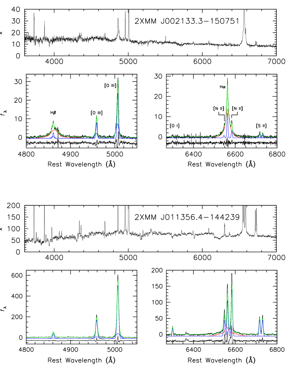
Figure 1: Magellan/MagE spectra of the sample, shifted to the rest-frame and corrected for Galactic extinction. The top panel focuses on the broad-band continuum features; the spectra have been slightly binned for the purposes of the display. The bottom panels highlight the major emission lines of interest. The black histogram is the observed emission-line spectrum, after subtraction of a featureless AGN continuum, Fe II emission, and host galaxy starlight. Multi-component decomposition of the emission lines are shown in blue for the narrow lines and in red for broad H$\alpha$ and H$\beta$ (offset vertically by an arbitrary constant for clarity); the final model is plotted in green. The bottom spectrum shows the residuals of the fit, also offset slightly vertically for clarity.

Figure 1: Figure 1, continued.

Figure 1: Figure 1, continued.

Figure 1: Figure 1, continued.

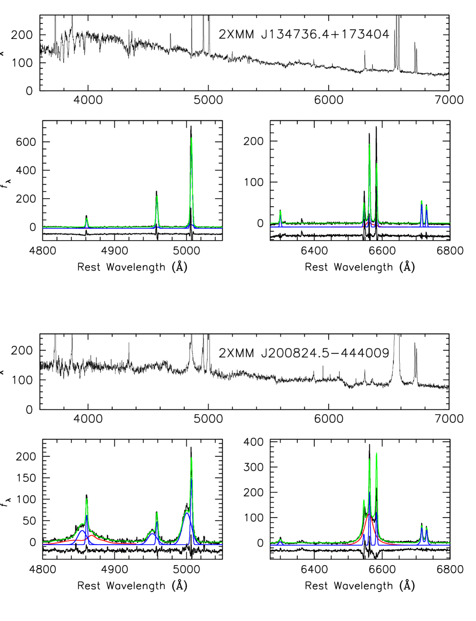
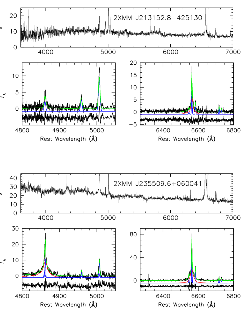
Figure 1: Figure 1, continued.

Figure 1: Figure 1, continued.

Detection of the Ca II IR triplets in 2XMMi J032459.9$-$025612, 2XMM J134736.4+173404, and 2XMM J200824.5$-$444009. The black histograms plot the original data, and the red line is the best-fit spectrum of a broadened K0 III template star, which is shown on the bottom. The spectra have been normalized to unity and shifted vertically for the purposes of the display. Blue vertical tickmarks identify the Ca II IR triplets.

fitted parameters for the broad and narrow emission lines are listed in Tables 2 and 3, respectively.

The Ca II infrared (IR) triplets ($\lambda$$\lambda$$\lambda$8498, 8542, 8662) are ideal features for deriving stellar velocity dispersions, especially for composite stellar populations and AGN host galaxies, because of their relative insensitivity to template mismatch (Dressler 1984) and reduced contamination from nonstellar emission (Barth et al. 2002; Greene & Ho 2006a). The three sources with the lowest redshifts cover the Ca II IR triplets in

Comparison of the new virial BH masses derived from our new detections of broad H$\alpha$ emission with the BH masses estimated by Kamizasa et al. (2012) based on X-ray variability. The solid line denotes the 1:1 relation. The virial BH masses are assumed to have uncertainties of 0.5 dex.

The $M_{\rm BH}-\sigma_{*}$ relation (solid line with shaded 1$\sigma$ scatter) of inactive BHs detected via spatially resolved dynamics (black symbols; Kormendy & Ho 2013), of AGNs with BH masses measured through reverberation mapping (blue symbols; Ho & Kim 2014), and of the low-mass active BHs (red symbols; this paper). For the sake of clarity, error bars are not shown for the inactive sample. Classical bulges and ellipticals are plotted in dark color; pseudobulges are plotted in a lighter shade. We assume that the low-mass objects are hosted by pseudobulges. Their bulge $\sigma_{*}$ are mostly estimated through the width of the core of [O III] $\lambda$5007; the three objects with $\sigma_{*}$ directly measured using the Ca II IR triplets are highlighted with a solid red point.

their bandpass, and these features are detected clearly in all of them (Figure 2). We use the direct pixel-fitting method, as implemented in Ho et al. (2009), in conjunction with a K0 III velocity template star observed during the same observing run, to derive $\sigma_{*}=43.9\pm 4.3$ km s^-1 for 2XMMi J032459.9$-$025612, $\sigma_{*}=88.1\pm 5.7$ km s^-1 for 2XMM J134736.4+173404, and $\sigma_{*}=76.3\pm 7.9$ km s^-1 for 2XMM J200824.5$-$444009. The errors account for fitting uncertainties but not for uncertainties due to choice of velocity templates, as we did not observe a large number of stars. However, comparison with the previous work of Xiao et al. (2011), who studied similar objects using MagE in exactly the same instrumental setup, verifies that our error estimates ($\sim 10\%$) are realistic.

3 Broad H$\alpha$, Black Hole Masses, and Eddington Ratios

We detect unambiguous broad H$\alpha$ emission in all 12 sources and broad H$\beta$ emission in 8 out of 12, confirming that all are genuine type 1 AGNs. 2XMM J123103.2+110648 remains the only example of a pure type 2 source (Ho et al. 2012) in the sample of Kamizasa et al. (2012). The broad H$\alpha$ luminosities range from $\sim 10^{40}$ to $10^{42}$ erg s^-1, with a median value of $2.5\times 10^{41}$ erg s^-1, close to 1 order of magnitude less luminous than the peak of distribution of optically selected $z$ $\mathrel{\hbox{\hbox to0.0pt{\hbox{\lower 4.0pt\hbox{$\sim$}}\hss}\hbox{$<$}}}$ 0.35 type 1 AGNs (Greene & Ho 2007b), but similar to the subsample of type 1 AGNs with $M_{\rm BH}<2\times 10^{6}$ $M_{\odot}$ (Greene & Ho 2007c). Given the low-mass selection of our sample, it is not surprising that the widths of broad H$\alpha$ are low (median FWHM = 934 km s^-1), well below the fiducial threshold of 2000 km s^-1 for narrow-line Seyfert 1 galaxies (Osterbrock & Pogge 1985).

The broad H$\alpha$ measurements afford us the opportunity to reevaluate the BH masses and Eddington ratios of the sample.

We estimate virial BH masses using the formalism for single-epoch spectra, recently recalibrated for the H$\beta$ line by Ho & Kim (2015), which takes into consideration the dependence of the virial coefficient (so-called $f$-factor) on bulge type (Ho & Kim 2014), as well as the latest updates to the $M_{\rm BH}-\sigma_{*}$ relation of inactive galaxies (Kormendy & Ho 2013), on which the calibration of the $f$-factor is based. As our sample specifically targets low-mass BHs, we expect, from experience with other similar samples (Greene et al. 2008; Jiang et al. 2011b), that the host galaxies contain pseudobulges. The BH mass estimator of Ho & Kim (2015) is based on the FWHM of broad H$\beta$ and the AGN continuum luminosity at 5100 Å, whereas the primary measurements in this study come from the FWHM and luminosity of broad H$\alpha$. Greene & Ho (2005b) show that the

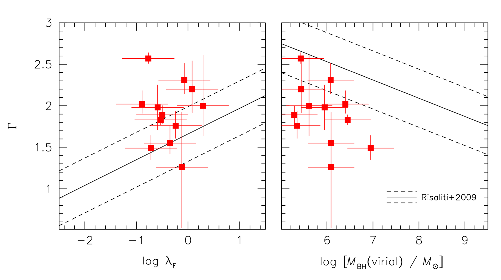
Figure 5: Variation of X-ray photon index, $\Gamma$, calculated over the 2–10 keV band (Kamizasa et al. 2012), with (left) Eddington ratio and (right) BH mass. The solid line is the best-fitting relation from Risaliti et al. (2009), with the 1 $\sigma$ scatter denoted by the two dashed lines.

line widths of broad H$\alpha$ and H$\beta$ scale closely with each other, as do the luminosities of the optical continuum and broad H$\alpha$. Adopting the empirical correlations of Greene & Ho (2005b, their equations 1 and 3), equation 4 of Ho & Kim (2015) becomes

$$\log\left(\frac{M_{\rm BH}}{M_{\odot}}\right)=2.06\log\left(\frac{{\rm FWHM_{{\rm H}\alpha}}}{1000\,{\rm km\,s^{-1}}}\right)+$$ (1)

$$0.46\log\left(\frac{L_{{\rm H}\alpha,b}}{10^{42}\,{\rm erg\,s^{-1}}}\right)+k,$$

where $k=6.76$ for classical bulges and $k=6.35$ for pseudobulges. In this paper, we adopt the zero point for pseudobulges. The uncertainty on the masses is $\sim 0.5$ dex, based on the intrinsic scatter of the empirical calibrations (Ho & Kim 2014, 2015).

The new masses range from $M_{\rm BH}\approx 1.9\times 10^{5}$ to $8.3\times 10^{6}$ $M_{\odot}$, with a median value of $1.2\times 10^{6}$ $M_{\odot}$. This confirms that the selection method of Kamizasa et al. (2012), based on X-ray variability, indeed does isolate low-mass BHs effectively. However, a direct comparison between their X-ray–based masses and ours (Figure 3) reveals large discrepancies. Whereas the virial masses span nearly 2 dex, most of the X-ray–based masses are confined to a very narrow range of only $\sim 0.3$ dex. Moreover, the scatter is not random: the X-ray–based masses are systematically higher than the virial masses, on average by $\sim 0.4$ dex. While large uncertainties no doubt enter into the virial mass estimates, especially in the low-mass regime where the empirical calibrations remain poorly tested, we have reasonable confidence that our derived masses are not affected by large, systematic biases because they more-or-less follow the $M_{\rm BH}-\sigma_{*}$ relation, at least within the relatively large scatter in the pseudobulge regime of the correlation (Figure 4). This has been established for other samples of low-mass type 1 AGNs (Barth et al. 2005; Greene & Ho 2006b; Xiao et al. 2011; see also Jiang et al. 2011a). For the present analysis, we only have direct stellar velocity dispersions for three sources (Section 2); as for the rest, we assume $\sigma_{*}={\rm FWHM_{[O~{}III]}/2.35}$ (appropriate for a Gaussian profile), where ${\rm FWHM_{[O~{}III]}}$ pertains to the core of the line. This approximation has been shown to be valid (Nelson & Whittle 1996; Greene & Ho 2005a), especially for lower-ionization lines such as [S II] or [N II] (Ho 2009). The [S II] and [O III] lines of our sample have very similar FWHM values, and so we choose the measurements based on the stronger [O III] line.

The offset between the virial and X-ray–based BH masses can be compensated by adopting in equation 1 the zero point for classical bulges instead of pseudobulges, which differs by precisely this amount ($\sim 0.4$ dex). However, as discussed above, we have strong reason to believe that these low-mass AGNs are hosted by pseudobulges.

Next, we convert the broad H$\alpha$ luminosities to bolometric luminosities, using the $L_{{\rm H}\alpha,b}-L_{\rm 5100~{}\AA}$ relation of Greene & Ho (2007c) and a canonical bolometric correction of $L_{\rm bol}=9.8L_{\rm 5100~{}\AA}$ (McLure & Dunlop 2004). The resulting Eddington ratios are surprisingly high ($\lambda_{\rm E}\approx 0.1-2$; median $\lambda_{\rm E}=0.44$), not dissimilar from the optically selected sample of Greene & Ho (2007c). The bolometric luminosity can be estimated alternatively from the available X-ray luminosity, using a luminosity-dependent X-ray bolometric correction factor (Ho 2008). Adopting $L_{\rm bol}=20L_{\rm X}$ for the 2–10 keV band (Vasudevan & Fabian 2007), we find consistent values of $\lambda_{\rm E}\approx 0.1-1$, with a median value of $\lambda_{\rm E}=0.38$.

We note, in agreement with Kamizasa et al. (2012), that the hard X-ray (2–10 keV) photon index does not correlate with BH mass or Eddington ratio in the manner predicted from extrapolation of AGN samples of higher mass and luminosity (Fig. 5).

Line-ratio diagnostic diagram of [O III] $\lambda$5007/H$\beta$ versus [N II] $\lambda$6583/H$\alpha$. The small black points are Sloan Digital Sky Survey measurements from Kauffmann et al. (2003) with S/N larger than 6. The new sample of 12 objects studied in this paper are plotted as large red squares; J1231+1106, from Ho et al. (2012), is marked with an additional cross. Conservative errors of $\sim 20\%$ are assigned to our line ratio measurements. Small open red squares are low-mass type 2 Seyferts from Barth et al. (2008), while the type 1 sample of Greene & Ho (2007c) is shown as open blue circles. NGC 4395 and POX 52 (Barth et al. 2004) are plotted as a filled green triangle and circle, respectively. Star-forming galaxies are located to the left of the dashed line, AGNs are found to the right of the solid line, and composite sources lie in between (Kewley et al. 2006).

4 Constraints on Star Formation Rate

The spectra exhibit a rich set of narrow emission lines generally consistent with AGN photoionization. On the [O III] $\lambda$5007/H$\beta$ versus [N II] $\lambda$6583/H$\alpha$ diagnostic diagram (Figure 6), most of the objects lie in the region intermediate between high-excitation star-forming galaxies and classical Seyferts, a manifestation of the relatively low metallicity associated with the lower-mass host galaxies in our study (Ludwig et al. 2012). Our sources overlap well with other samples of type 1 (Barth et al. 2004; Greene & Ho 2004, 2007c) and type 2 (Barth et al. 2008) low-mass AGNs. As was found for the Greene & Ho (2007c) sample, some of the sources in our sample (5/13) have narrow-line intensity ratios that formally place them in the territory of star-forming galaxies. We suspect that star formation contaminates the integrated spectra of these objects, and possibly others in our sample.

Can the star formation rate (SFR) be constrained in these systems? Ho (2005) proposed that the strength of [O II] $\lambda$3727, normally a widely used SFR indicator in star-forming galaxies at intermediate redshifts, can also be utilized for this purpose in AGNs. The fundamental premise behind this idea is that, while the narrow-line regions of AGNs certainly also emit [O II], the level of [O II] emission in high-excitation sources (i.e. Seyferts and quasars) is well-constrained by the level of [O III] $\lambda$5007, which can be directly observed. The intensity ratio [O II]/[O III], which varies strongly with the ionization parameter, decreases with increasing [O III] luminosity (Kim et al. 2006). To zeroth order, all of the [O III] emission in luminous AGNs comes from nonstellar photoionization. Star

Correlation between intrinsic soft X-ray luminosity in the 0.5–2 keV band and extinction-corrected [O III] $\lambda$5007 luminosity for the 12 objects in this paper (filled red squares), 2XMM J123103.2+110648 (filled red square with cross; Ho et al. 2012), low-mass type 2 AGNs (open red squares; Thornton et al. 2009); low-mass type 1 AGNs (open blue circles; Greene & Ho 2007a; Desroches et al. 2009; Dong et al. 2012a), NGC 4395 (filled green triangle; Panessa et al. 2006, adjusted to a distance of 4.3 Mpc), and POX 52 (solid green circle; Thornton et al. 2008). The solid line is the best-fitting relation from Panessa et al. (2006), with the 1 $\sigma$ scatter denoted by the two dashed lines; their X-ray luminosities were transformed from the 2–10 keV band to the 0.5–2 keV band assuming a photon index of $\Gamma=1.8$. For the objects studied in this paper and in Ho et al. (2012), we conservatively assign a uncertainty of 0.3 dex for the $L_{\rm[O~{}III]}$. The five objects with “excess [O III] emission are highlighted with a cyan center.

formation, if present, contributes negligibly to [O III] because the host galaxies, being massive in general for luminous Seyferts and quasars, should have high metallicity (Tremonti et al. 2004). Thus, given an observed strength of [O III] in an AGN, its associated level of [O II] emission can be predicted, and any “excess” beyond that can be attributed to star formation (Ho 2005; Kim et al. 2006).

The [O II]-based technique to measure SFRs in AGNs depends on a critical condition: that the host galaxy has high metallicity. Unfortunately, this requirement breaks down for low-mass galaxies, and, at sufficiently high redshifts, even for high-mass galaxies. O-star photoionization of low-metallicity gas produces high-excitation H II regions, which, like AGNs, emit strong [O III] $\lambda$5007 (Osterbrock 1989). Here, we suggest that this difficulty can be circumvented with the help of an additional constraint from X-ray observations. The extinction-corrected [O III] luminosity of Compton-thin AGNs correlates well with the intrinsic X-ray luminosity (Bassani et al. 1999), over a wide range of luminosities and masses (Panessa et al. 2006; Stern & Laor 2012), including optically selected low-mass AGNs (Dong et al. 2009; Ho et al. 2012). Hence, provided that a robust X-ray detection is available, we can deduce roughly the corresponding [O III] luminosity that should be associated with the AGN, and thereby also its fractional contribution to the [O II] emission.

Figure 7 confirms that some of the objects in the current sample of AGNs selected by X-ray variability indeed do depart systematically from the canonical $L_{\rm X}-L_{\rm[O~{}III]}$ correlation. For

Dependence of [O II]/[O III] ratio on extincton-corrected [O III] luminosity. The solid line is the empirical relation derived from a large sample of type 1 AGNs selected from the Sloan Digital Sky Survey (Kim et al. 2006). Most of the sample lies systematically above the relation, expecially the five sources that deviate the most from the $L_{\rm X}-L_{\rm[O~{}III]}$ correlation (Figure 7), in the sense that at a given [O III] luminosity there is “extra” [O II] emission, which we argue originates from and hence traces star formation in the host galaxy.

illustrative purposes, we highlight (red squares with cyan centers) the five objects that formally lie outside the 1$\sigma$ scatter of the $L_{\rm X}-L_{\rm[O~{}III]}$ relation of Panessa et al. (2006), in the sense that at a given X-ray luminosity they are overluminous in [O III] by a factor of $\sim 3$. This is to be expected, if, as we suspect, high-excitation H II regions contribute to the integrated [O III] emission in our sample of low-mass AGNs, which most likely live in low-mass, low-metallicity host galaxies. These very same five objects stand out as having systematically higher [O II]/[O III] ratios for their [O III] luminosities (Figure 8), indicating that star formation contributes to their [O II] emission. (Interestingly, however, they do not stand out in any obvious way in the traditional dignostic diagram in Figure 6.)

We apply the above procedure to derive “AGN-decontaminated” [O II] luminosities for our objects. As in Ho (2005), we use the empirical calibration of Kewley et al. (2004) to derive SFRs from $L_{\rm[O~{}II]}$, adopting, for concreteness, a metallicity of 0.5 solar. Most objects have rather modest SFRs ($\mathrel{\hbox{\hbox to0.0pt{\hbox{\lower 4.0pt\hbox{$\sim$}}\hss}\hbox{$<$}}}$ 1 $M_{\odot}$ yr^-1; Table 4).

5 The Peculiar Narrow-line Kinematics of 2XMM J200824.5$-$444009

We draw attention to the highly unusual kinematics of the narrow emission lines in 2XMM J200824.5$-$444009 (Figure 1). The profile of [O III] $\lambda$$\lambda$4959, 5007 qualifies the source as “double-peaked”, but in other objects of this class the two components typically have comparable widths (e.g., Liu et al. 2010; Smith et al. 2010; Shen et al. 2011; Comerford et al. 2012; Ge et al. 2012). Here, the two components have very different profiles: a sharp, core with FWHM = 175 km s^-1 plus an extremely broad component with FWHM = 870 km s^-1 blueshifted by 381 km s^-1. This characteristic double-component structure is clearly present in H$\beta$, and, although less obvious visually, also in [S II]. It is crucial to properly account for this complex narrow-line profle to deblend narrow H$\alpha$ and [N II], in order to obtain an accurate measurement of broad H$\alpha$.

6 Summary

AGNs with $M_{\rm BH}$ $\mathrel{\hbox{\hbox to0.0pt{\hbox{\lower 4.0pt\hbox{$\sim$}}\hss}\hbox{$<$}}}$ $10^{6}$ $M_{\odot}$ are an important constituent for understanding the full demography of central BHs. The vast majority of currently known low-mass AGNs derive from optical selection. In a recent study, Kamizasa et al. (2012) presented a sample of candidate low-mass BHs based on X-ray variability characteristics. We used the Magellan 6.5m Clay telescope to obtain high-quality, optical echellette spectra of 12 out of the 15 sources from Kamizasa’s sample. Broad H$\alpha$ emission is unambiguously detected in all the objects, permitting us to calculate robust virial BH masses and Eddington ratios. We confirm that the sample contains low-mass BHs accreting at a high fraction of their Eddington rate: median $M_{\rm BH}$ $\approx$ $1.2\times 10^{6}$ $M_{\odot}$; median $\lambda_{\rm E}=0.44$. Assuming the AGNs to be hosted by pseudobulges, our BH masses are significantly and systematically larger than those estimated from X-ray variability. The moderately high resolution of our spectra allow us to measure the central velocity dispersion of the host galaxies, either directly from stars or indirectly from ionized gas. We show that the virial BH masses follow the $M_{\rm BH}-\sigma_{*}$ relation of pseudobulges. Lastly, we argue that at least some of the objects have ongoing star formation, and we introduce a method to estimate the SFRs of low-metallicity AGN host galaxies based on measurements of X-rays and optical emission lines.

References

- (1) Araya Salvo, C., Mathur, S., Ghosh, H., Fiore, F., & Ferrarese, L. 2012, ApJ, 757, 179
- (2) Baldassare, V. F., Reines, A., Gallo, E., & Greene, J. 2015, ApJ, 809, L14
- (3) Barth, A. J., Greene, J. E., & Ho, L. C. 2005, ApJ, 619, L151
- (4) Barth, A. J., Greene, J. E., & Ho, L. C. 2008, AJ, 136, 1179
- (5) Barth, A. J., Ho, L. C., Rutledge, R. E., & Sargent, W. L. W. 2004, ApJ, 607, 90
- (6) Barth, A. J., Ho, L. C., & Sargent, W. L. W. 2002, AJ, 124, 2607
- (7) Bassani, L., Dadina, M., Maiolino, R., et al. 1999, ApJS, 121, 473
- (8) Cardelli, J. A., Clayton, G. C., & Mathis, J. S. 1989, ApJ, 345, 245
- (9) Comerford, J. M., Gerke, B. F., Stern, D., et al. 2012, ApJ, 753, 42
- (10) Desroches, L.-B., Greene, J. E., & Ho, L. C. 2009, ApJ, 698, 1515
- (11) Desroches, L.-B., & Ho, L. C. 2009, ApJ, 690, 267
- (12) Dong, R., Greene, J. E., & Ho, L. C. 2012a, ApJ, 761, 73
- (13) Dong, X.-B., Ho, L. C., Yuan, W., et al. 2012b, ApJ, 755, 167
- (14) Dressler, A. 1984, ApJ, 286, 97
- (15) Filippenko, A. V., & Ho, L. C. 2003, ApJ, 588, L13
- (16) Ge, J.-Q., Hu, C., Wang, J.-M., Bai, J.-M., & Zhang, S. 2012, ApJS, 201, 32
- (17) Goulding, A., & Alexander, D. 2009, MNRAS, 398, 1165
- (18) Greene, J. E., & Ho, L. C. 2004, ApJ, 610, 722
- (19) Greene, J. E., & Ho, L. C. 2005a, ApJ, 627, 721
- (20) Greene, J. E., & Ho, L. C. 2005b, ApJ, 630, 122
- (21) Greene, J. E., & Ho, L. C. 2006a, ApJ, 641, 117
- (22) Greene, J. E., & Ho, L. C. 2006b, ApJ, 641, L21
- (23) Greene, J. E., & Ho, L. C. 2007a, ApJ, 656, 84
- (24) Greene, J. E., & Ho, L. C. 2007b, ApJ, 667, 131
- (25) Greene, J. E., & Ho, L. C. 2007c, ApJ, 670, 92
- (26) Greene, J. E., Ho, L. C., & Barth, A. J. 2008, ApJ, 688, 159
- (27) Gültekin, K., Richstone, D. O., Gebhardt, K., et al. 2009, ApJ, 698, 198
- (28) Halpern, J. P., & Steiner, J. E. 1983, ApJ, 269, L37
- (29) Ho, L. C. 2005, ApJ, 629, 680
- (30) Ho, L. C. 2008, ARA&A, 46, 475
- (31) Ho, L. C. 2009, ApJ, 699, 638
- (32) Ho, L. C., Filippenko, A. V., Sargent, W. L. W., & Peng, C. Y. 1997, ApJS, 112, 391
- (33) Ho, L. C., Greene, J. E., Filippenko, A. V., & Sargent, W. L. W. 2009, ApJS, 183, 1
- (34) Ho, L. C., & Kim, M. 2009, ApJS, 184, 398
- (35) Ho, L. C., & Kim, M. 2014, ApJ, 789, 17
- (36) Ho, L. C., & Kim, M. 2015, ApJ, 809, 123
- (37) Ho, L. C., Kim, M., & Terashima, Y. 2012, ApJ, 759, L16
- (38) Jiang, Y.-F., Greene, J. E., & Ho, L. C. 2011a, ApJ, 737, L45
- (39) Jiang, Y.-F., Greene, J. E., Ho, L. C., Xiao, T., & Barth, A. J. 2011b, ApJ, 742, 68
- (40) Kamizasa, N., Terashima, Y., & Awaki, H. 2012, ApJ, 751, 39
- (41) Kauffmann, G., Heckman, T. M., Tremonti, C., et al. 2003, MNRAS, 346, 1055
- (42) Kewley, L. J., Geller, M. J., & Jansen, R. A. 2004, AJ, 127, 2002
- (43) Kewley, L. J., Groves, B., Kauffmann, G., & Heckman, T. 2006, MNRAS, 372, 961
- (44) Kim, M., Ho, L. C., & Im, M. 2006, ApJ, 642, 702
- (45) Kormendy, J., & Ho, L. C. 2013, ARA&A, 51, 511
- (46) Lemons, S., Reines, A., Plotkin, R., Gallo, E., & Greene, J. 2015, ApJ, 805, 12
- (47) Liu, X., Shen, Y., Strauss, M. A., & Greene, J. E. 2010, ApJ, 708, 427
- (48) Lu, Y., & Yu, Q. 2001, MNRAS, 324, 653
- (49) Ludwig, R. R., Greene, J. E., Barth, A. J., & Ho, L. C. 2012, ApJ, 756, 51
- (50) Marshall, J. L., Burles, S., Thompson, I. B., et al. 2008, Proc. SPIE, 7014
- (51) McConnell, N. J., & Ma, C.-P. 2013, ApJ, 764, 184
- (52) McHardy, I. M., Körding, E., Knigge, C., Uttley, P., & Fender, R. P. 2006, Nature, 444, 730
- (53) McLure, R. J., & Dunlop, J. S. 2004, MNRAS, 352, 1390
- (54) Moran, E. C., Shahinyan, K., Sugarman, H. R., Velez, D. O., & Eracleous, M. 2014, AJ, 148, 136
- (55) Nelson, C. H., & Whittle, M. 1996, ApJ, 465, 96
- (56) Osterbrock, D. E. 1989, Astrophysics of Gaseous Nebulae and Active Galactic Nuclei (Mill Valley: Univ. Science Books)
- (57) Osterbrock, D. E., & Pogge, R. W. 1985, ApJ, 297, 166
- (58) Panessa, F., Bassani, L., Cappi, M., et al. 2006, A&A, 455, 173
- (59) Papadakis, I. E. 2004, MNRAS, 348, 207
- (60) Reines, A. E., Greene, J. E., & Geha, M. 2013, ApJ, 775, 116
- (61) Reines, A. E., Plotkin, R., Russell, T., et al. 2014, ApJ, 787, L30
- (62) Reines, A. E., Sivakoff, G. R., Johnson, K. E., & Brogan, C. L. 2011, Nature, 470, 66
- (63) Satyapal, S., Böker, T., Mcalpine, W., et al. 2009, ApJ, 704, 439
- (64) Satyapal, S., Secrest, N. J., McAlpine, W., et al. 2014, ApJ, 784, 113
- (65) Satyapal, S., Vega, D., Dudik, R. P., Abel, N. P., & Heckman, T. 2008, ApJ, 677, 926
- (66) Schlafly, E. F., & Finkbeiner, D. P. 2011, ApJ, 737, 103
- (67) Schramm, M., Silverman, J. D., Greene, J. E., et al. 2013, ApJ, 773, 150
- (68) Seth, A. C., Cappellari, M., Neumayer, N., et al. 2010, ApJ, 714, 71
- (69) Shen, Y., Liu, X., Greene, J. E., & Strauss, M. 2011, ApJ, 735, 48
- (70) Smith, K. L., Shields, G. A., Bonning, E. W., et al. 2010, ApJ, 716, 866
- (71) Stern, J., & Laor, A. 2012, MNRAS, 426, 2703
- (72) Terashima, Y., Kamizasa, N., Awaki, H., Kubota, A., & Ueda, Y. 2012, ApJ, 752, 154
- (73) Thornton, C. E., Barth, A. J., Ho, L. C., Rutledge, R. E., & Greene, J. E. 2008, ApJ, 686, 892
- (74) Thornton, C. E., Barth, A. J., Ho, L. C., & Greene, J. E. 2009, ApJ, 705, 1196
- (75) Tremonti, C. A., Heckman, T. M., Kauffmann, G., et al. 2004, ApJ, 613, 898
- (76) Vasudevan, R. V., & Fabian, A. C. 2007, MNRAS, 381, 1235
- (77) Watson, M. G., Schröder, A. C., Fyfe, D., et al. 2009, A&A, 493, 339
- (78) Xiao, T., Barth, A. J., Greene, J. E., et al. 2011, ApJ, 739, 28
- (79) Zhang, W. M., Soria, R., Zhang, S. N., Swartz, D. A., & Liu, J. F. 2009, ApJ, 699, 281