Abundance analysis of SDSS J134338.67+484426.6; an extremely metal-poor star from the SDSS-MARVELS pre-survey

Abundance analysis of SDSS J134338.67+484426.6; an extremely metal-poor star from the MARVELS pre-survey

Abstract

We present an elemental-abundance analysis of an extremely metal-poor (EMP; [Fe/H] $<-3.0$) star, SDSS J134338.67+484426.6, identified during the course of the MARVELS spectroscopic pre-survey of some 20000 stars to identify suitable candidates for exoplanet searches. This star, with an apparent magnitude $V=12.14$, is the lowest metallicity star found in the pre-survey, and is one of only $\sim$20 known EMP stars that are this bright or brighter. Our high-resolution spectroscopic analysis shows that this star is a subgiant with [Fe/H] = $-3.42$, having ”normal” carbon and no enhancement of neutron-capture abundances. Strontium is under-abundant, [Sr/Fe] $=-0.47$, but the derived lower limit on [Sr/Ba] indicates that Sr is likely enhanced relative to Ba. This star belongs to the sparsely populated class of $\alpha$-poor EMP stars that exhibit low ratios of [Mg/Fe], [Si/Fe], and [Ca/Fe] compared to typical halo stars at similar metallicity. The observed variations in radial velocity from several epochs of (low- and high-resolution) spectroscopic follow-up indicate that SDSS J134338.67+484426.6 is a possible long-period binary. We also discuss the abundance trends in EMP stars for $r$-process elements, and compare with other magnesium-poor stars.

1 Introduction

Extremely metal-poor (EMP; [Fe/H] $<-3.0$) stars were formed during the very early phases of our Galaxy’s evolution, and thus carry the chemical imprints of the first generations of supernovae that exploded in the Galaxy (Bromm, Yoshida & Hernquist, 2003; Kobayashi et al., 2006). Detailed abundance analysis of such stars constrain the nuclear processes and nucleosynthesis sites which were prevalent during early galaxy evolution, and can be used to explore predictions of Galactic chemical-evolution models (Hansen, Montes & Arcones, 2014).

EMP stars exhibit a variety of distinct abundance patterns (for detailed reviews see Beers & Christlieb 2005; Frebel & Norris 2015). High-resolution spectroscopic surveys using 8-10 m class telescopes have revealed a number of interesting trends in the abundance ratios of these stars (Cayrel et al., 2004; Barklem et al., 2005; Lai et al., 2008; Yong et al., 2013; Roederer et al., 2014). For example, François et al. (2007) showed that there exists a large scatter in the [n-capture/Fe] ratios for stars with [Fe/H] $<-2.5$, while the $\alpha$-elements and iron-peak elements exhibit a surprisingly uniform behaviour. These authors also showed that the light n-capture element abundances (e.g., Sr) are anti-correlated with the abundances of heavier species such as Ba, suggesting the operation of the so-called Light Element Primary Process (LEPP) among some stars of extremely low metallicity (Montes et al., 2007). As these trends were derived from samples of stars that did not exhibit other anomalies in their abundance ratios, they may be representative of the well-mixed ISM abundance at these metallicities. Similar results have been observed in other well-mixed environments, such as globular-cluster stars (Otsuki et al., 2006).

The majority of EMP stars in the halo and nearby dwarf galaxies exhibit low scatter in their $\alpha$-elements, although a few exhibit abnormally low values compared to the the mean halo $\alpha$-element abundance (Carney et al., 1997; King, 1997; Lai et al., 2009; Aoki et al., 2009; Tafelmeyer et al., 2010; Kirby & Cohen, 2012; Cohen et al., 2013). Recently, Caffau et al. (2013) identified a class of $\alpha$-poor EMP stars, several of which exhibit low carbon abundances as well (see also Cohen et al. 2013, and references therein).

Kobayashi et al. (2014) showed that $\alpha$-poor EMP stars can be naturally explained by the nucleosynthesis yields of core-collapse supernovae, i.e., 13 - 25 M_⊙ supernovae or hypernovae, but pointed out that detailed abundances of additional iron-peak elements, which are not available for most of this subset of EMP stars, are required to better constrain the models.

According to Ivans et al. (2003), the low $\alpha$-element abundances exhibited by stars in their sample are due to the the larger contribution of SNIa yields over the pre-existing SNeII ejecta. However, EMP stars might have formed much earlier than the onset of SNIa. So it is less likely that the EMP stars are affected by the SNe Ia yields unless they belong to a system where the star formation rate is very low (and mixing is highly inhomogenous), so as to keep the gas cloud low in metallicity until further star formation has taken place (after the onset of SNe Ia).

In this paper we report low- and high-resolution spectroscopic follow-up observations of a newly identified EMP star, SDSS J134338.67+484426.6 (hereafter, SDSS J1343+4844) that may shed additional light on the nature of early nucleosynthesis in the Galaxy, in particular for stars that do not exhibit other abundance anomalies (such as carbon over-abundances) that are commonly found for EMP stars. Since SDSS J1343+4844 is bright compared to many of the known EMP stars, particularly among the rare $\alpha$-poor sub-class, it also presents an ideal target for future high-resolution studies capable of deriving detailed isotopic ratios, which can be used to better constrain the SNe models.

2 Observation and data reduction

SDSS J1343+4844 was identified as a likely metal-poor star from SDSS-III-MARVELS (Multi-object APO Radial Velocity Exoplanet Large-area Survey; Ge et al. 2008) pre-survey spectroscopy using the SDSS legacy spectrographs (Gunn et al., 2006). The pre-survey was used for selecting suitable bright dwarfs for planet searches, in the magnitude range 9 $<$ V $<$ 13 and with spectral types from late F to K. MARVELS pre-survey plates were reduced using a slightly modified version (NOCVS:v5_3_23) of the IDLSPEC2D pipeline. Stellar atmospheric parameters were estimated using the n-SSPP pipeline, a modified version of the SEGUE Stellar Parameter Pipeline (SSPP; Lee et al. 2008, see also Beers et al. 2014 for a description of the use of the n-SSPP). Based on the pipeline procedures and visual inspection, SDSS J1343+4844 was identified as a carbon-normal EMP star.

Figure 1 shows the metallicity distribution of the complete set of MARVELS pre-survey stars; these stars clearly exhibit peak metallicities arising from the thin-disk and thick-disk components of the Galaxy. As is clear from inspection of this figure, metal-poor stars are quite rare in the sample, due to the low Galactic latitude of the pre-survey area. Among the MARVELS pre-survey spectroscopic spectra (N $\sim$ 20000), SDSS J1343+4844 was the only star found with metallicity [Fe/H] $<-3.0$.

Follow up high-resolution ($R\sim 30000$) spectroscopic observations of SDSS J1343+4844 were obtained with the ARC Echelle Spectrograph on the 3.5-m telescope at Apache Point Observatory (APO) and the High resolution Spectrograph (HRS) on the Hobby-Eberly 9.2-m telescope (HET). We also obtained multi-epoch low-resoluion ($R\sim 1300$) spectra using the Hanle Faint Object Spectrograph Camera (HFOSC) at the 2-m Himalayan Chandra Telescope (HCT). The spectral resolution, wavelength coverage, and the signal-to-noise ratios of the available spectra are listed in Table 1.

The APO pipeline-reduced high-resolution spectrum exhibited slightly lower equivalent widths compared to the HET data. Thus, we manually re-reduced the data using IRAF, in order to ensure proper background subtraction, and found a better match between the equivalent widths of the APO and HET datasets in the overlapping wavelength regions (see Figure 2). The equivalent widths for individual species are listed in the table in the appendix.

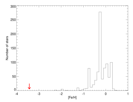
Figure 1: Metallicity distribution of the MARVELS pre-survey stars. The two strong peaks correspond to the expected metallicities of the Galactic thin and thick disks. The arrow indicates the position of SDSS J1343+4844.

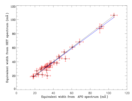
Figure 2: Comparison of measured equivalent widths of the spectral lines from the high-resolution APO and HET spectra. The solid line is a fit to these measurements; the dashed line is the one-to-one line.

Table 1: Details of observations and heliocentric radial velocities of SDSS J1343+4844 using various telescope/spectrograph combinations

Date	MJD	Telescope-Spectrograph	Resolving Power	$\lambda$ coverage (Å)	SNR∗	RV (km/s)
2009-01-14	54845.48138	SDSS-premarvels	2000	3800 - 9200	58	$-$114.7 $\pm$ 3.8
2009-03-20	54910.23972	APO-ARCES	31500	3373 - 10240	60	$-$123.2 $\pm$ 9.2
2012-04-23	56040.15483	HET-HRS	30000	4376 - 7838	58	$-$106.1 $\pm$ 4.0
2013-06-05	56448.84183	HCT-HFOSC	1330	3800 - 6840	133	$-$248.6 $\pm$ 10.4
2014-05-28	56805.84180	HCT-HFOSC	1330	3800 - 6840	156	$-$219.3 $\pm$ 10.9
2014-06-25	56833.91528	HCT-HFOSC	1330	3800 - 6840	141	$-$241.0 $\pm$ 10.9
2014-07-31	56869.67394	HCT-HFOSC	1330	3800 - 6840	136	$-$269.7 $\pm$ 10.9

^∗ SNR is calculated at 5000 Å.

3 Radial velocities

Radial velocities were calculated based on six epochs of high- and low-resolution data taken over a span of five years. A cross-correlation analysis was performed, using the best-matching synthetic template that represents the stellar parameters and the chemical abundances of SDSS J1343+4844, as derived below, and degraded to match the spectral resolution of each observation. These observed velocities were then corrected for Earth’s motion; the resultant heliocentric radial velocities are presented in Table 1.

A stability analysis of the HCT-HFOSC spectrograph was performed in order to estimate realistic errors for the derived radial velocities of this star. For this purpose, calibration exposures of FeAr, taken during the course of an entire night, were used. One of the lamp exposures was taken as a reference and relative radial velocities were derived. Although drifts in the calibration spectra for which the telescope position did not change are less than 2 km/sec, a large systematic shift of the spectra was noticed for a number of different telescope pointings; ranging from $-$30 km/s to $+$30 km/s. The systemic shift in the spectra due to the changing telescope position has been corrected using the prominent [OI] skylines at 5577.34, 6300.3, 6363.8 Å . We took the median of the shifts calculated from these lines and corrected all the spectra observed with HCT accordingly.

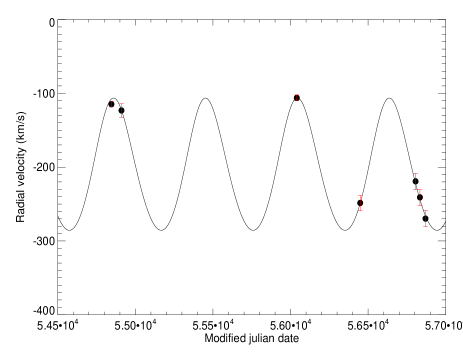
Figure 3: Variation of radial velocity with MJD. The black dots represent the observed points; the black line indicates the best-fit orbit, corresponding to a period of 592 days.

We made use of the software package RVLIN, provided by Wright & Howard (2009), which is a set of IDL routines to fit Keplerian orbits to the radial velocity data, and find the period of the radial-velocity variation. The radial-velocity measurements exhibit a variation with a period of 592 days; the best fit for is shown in Figure 3. Although the data are insufficient to derive the mass ratio of the binary system, the binary nature appears to be clear. Additional radial-velocity monitoring of this system would be useful to check on the derived period, given the sparse coverage of the proposed orbit at present.

4 Stellar parameters

Low- and high-resolution spectroscopic data were both used for deriving estimates of the effective temperature, log g, and metallicity, [Fe/H], for SDSS J1343+4844, as described below, so that these determinations might be compared with one another.

Stellar temperature estimates were derived making use, in part, of various available photometric datasets. The photometric colours and errors are listed in Table 3. A reddening estimation (E(B-V) = 0.009) from the Schlegel et al. dust maps (Schlegel, Finkbeiner & Davis, 1998) was used. Optical (APASS; Henden et al. 2015) and NIR (2MASS; Cutri et al. 2003) photometric data were used to derive effective temperature estimates, based on the Alonso relations (Alonso, Arribas & Martinez-Roger, 1996; Alonso, Arribas & Martínez-Roger, 1999) assuming a dwarf classification for a metallicity [Fe/H] = $-3.0$ (Table 2).

We also used VOSA (http://svo2.cab.inta-csic.es/), the online SED fitter to derive the temperature, using all of the available photometry (optical, 2MASS, and WISE, Wright et al. 2010). A Bayesian fit using the ATLAS-NOVER-NEWODF model yielded a best-fit value of T_eff = 5750 K.

We also fit the H_β line wings of the APO and HET spectra for various temperatures. The red wing of H_β in the APO spectrum lies close to the edge of an echelle order, so it was not considered in the fitting. The best-fit synthetic spectrum in this region, along with the observed spectra from APO and HET, are shown in Figure 4.

The derived temperature from the n-SSPP pipeline is 6161 K, which clearly deviates from the rest of the estimates. This is due, in part, to the fact that the flux calibration of the MARVELS pre-selection spectrum is not accurate, as these plug-plates were observed during twilight at high airmass. So, we re-derived T_eff using only the normalized SDSS spectrum, obtaining T_eff = 5832 K. An effective temperature of 5620 K was derived using the high-resolution spectra, employing the excitation equilibrium for the derived abundances using Fe I lines.

Finally, T_eff is also derived from the V-K colour, where the K_s magnitude is used instead of the K magnitude (the difference between the two magnitudes is K${}_{s}-$ K = $-0.0003$, which yields no difference in the derived temperature); we obtained T_eff = 5671 K. This estimate differs from the temperature obtained based on the excitation equillibrium approach by only 50 K, which we adopt for our subsequent analysis.

Table 2: Photometric data for SDSS J1343+4844

	B	V	J	H	Ks	W1	W2	W3	W4
Magnitude	12.685	12.147	11.031	10.675	10.609	10.566	10.563	10.56	8.808
error	0.041	0.039	0.022	0.028	0.022	0.023	0.020	0.081	$\dots$ ∗

^∗ The error is not available in the catalog.

Table 3: The temperature derived from various methods

Colour/Technique	$T_{eff}$ (K)
	(for Dwarf)
B$-$V = 0.538 $\pm$ 0.057	5618 $\pm$ 130
V$-$K = 1.538 $\pm$ 0.044	5671 $\pm$ 37
J$-$H = 0.356 $\pm$ 0.036	5444 $\pm$ 144
J$-$K = 0.422 $\pm$ 0.031	5394 $\pm$ 144
SED fitting	5750
SSPP	6161
SDSS normalized spectra	5832
High resolution spectra - Excitation equilibrium	5620

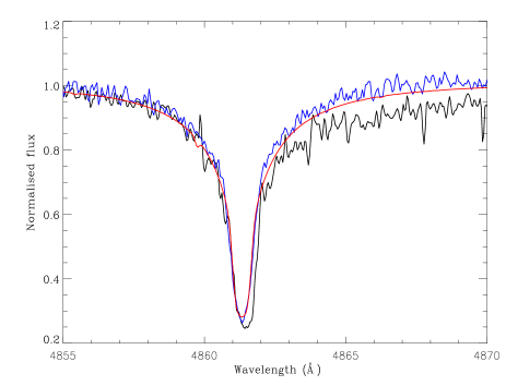
Figure 4: The H_β region from the APO spectrum (black), the HET spectrum (violet), and the synthesized spectrum (red) are shown. The best fit corresponds to $T_{eff}$ = 5620 K. The red wing of the APO spectrum falls at the edge of the echelle orders, so only the blue wing is considered for the fit.

We employ several different methods for the estimation of surface gravity of SDSS J1343+4844, including the ionization equilibrium of Fe I and Fe II lines, isochrone fitting, and the best-fit of the Mg I wings. We detected only four Fe II lines in the spectra, and derived log g = 3.44. Theoretical isochrones (Demarque et al., 2004) for an age range of 11-13 Gyr have been fitted by assuming a temperature of 5620 K, [Fe/H] = $-3.5$ and [$\alpha$/Fe] = 0. The log g values are taken where the temperature lines intersects the isochrones. There are two possibilities – the star could be a dwarf (log g $\sim$ 4.7) or a subgiant (log g $\sim$ 3.4). We also fit the Mg I lines for both the APO and HET spectra at $\lambda$5167 Å, $\lambda$5172 Å, and $\lambda$5183 Å for various values of log g, and obtained a value of log g = 3.4 (Figure 5). We adopt a value of log g = 3.4, a value that is consistent with all three methods.

The microturbulent velocity ($\xi$) of the star is derived using 60 Fe I lines, by adjusting the input microturbulence value in such a way that the weak and strong Fe I lines give the same abundances. The adopted stellar atmospheric parameters are listed in Table 4.

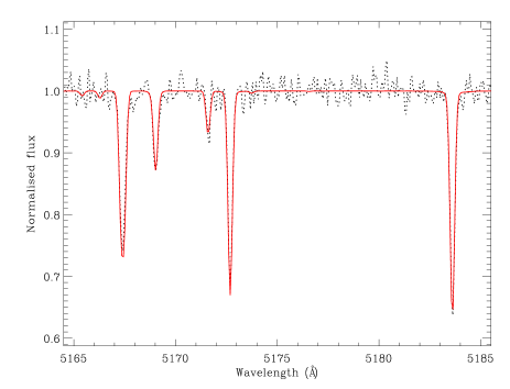
Figure 5: High-resolution HET spectrum in the region of the Mg I triplet. The black dashed line indicates the HET spectrum, while the red solid line indicates the synthetic spectrum with parameters corresponding to $T_{eff}$ = 5620 K, log g = 3.4. and [Fe/H] = $-3.42$.

4.1 Abundance analysis

We have used the ATLAS9 NEWODF (Castelli & Kurucz, 2004) model atmospheres without convective overshooting. The main abundance analysis results come from the APO spectrum, since it covers a broader wavelength region. In the overlapping regions of both the APO and HET spectra, a final abundance value is derived using a weighted average of abundances from both spectra. For the H_β and Mg fitting, the HET spectrum is primarily used because these lines fall at the edge of the echelle orders, and in such cases continuum normalization was better accomplished from the HET spectrum. We considered only lines with equivalent widths less than 100 mÅ for the abundance analysis, since they are on the linear part of the curve of growth, and are relatively insensitive to the choice of microturbulence.

We have adopted the solar abundance from Grevesse & Sauval (1998); solar isotopic fractions were used for all the elements. We used the CH linelist compiled by Masseron (private communication) and CN molecular line list compiled by Plez et al. (2005), and the NH and C₂ molecular-line lists from the Kurucz database. The atomic data for the other lines have been listed in the appendix along with the respective references used. The line lists used are the same as in Cui, Sivarani & Christlieb (2013). We employed version 12 of the turbospectrum code for spectrum synthesis and abundance analysis (Alvarez & Plez, 1998; Plez, 2012).

Table 4: The adopted stellar parameters for SDSS J1343+4844

$T_{eff}$	logg	$\xi$	[Fe/H]
(K)	(cgs)	(km/s)	dex
5620	3.44	1.45	$-3.42$

Table 5: Elemental abundance determinations for SDSS J1343+4844

Species	$N_{lines}$	A(X)	Solar	[X/H]	[X/Fe]#	$\sigma^{*}$
CH	…	5.52	8.52	$-$3.0	$+$0.42	synth
Na I	2	2.32	6.33	$-$4.01	$-$0.59§	0.01
Mg I	3	4.31	7.58	$-$3.27	$+$0.15	0.02
Al I	2	3.30	6.47	$-$3.15	$+$0.25§	0.07
Si I	1	4.11	7.55	$-$3.44	$-$0.02	…
S  I	…	$<$5.64	7.33	$<-$1.69	$<+$1.73†	synth
Ca I	4	3.13	6.36	$-$3.23	$+$0.19	0.16
Sc II	1	$-0.08$	3.17	$-$3.25	$+$0.17	…
Ti II	11	1.98	5.02	$-$3.04	$+$0.38	0.25
Cr I	2	2.28	5.67	$-$3.39	$+$0.03	0.04
Mn I	2	1.75	5.39	$-$3.64	$-$0.22	0.10
Fe I	60	4.08	7.50	$-$3.42	0.00	0.19
Fe II	4	4.37	7.50	$-$3.13	0.29	0.08
Ni I	3	3.15	6.25	$-$3.10	$+$0.32	0.10
Sr II	2	$-0.92$	2.97	$-$3.89	$-$0.47	0.12
Ba II	…	$<-1.83$	2.13	$<-$3.96	$<-$0.54†	synth

^§ Represents the values after applying the NLTE corrections.
^† Denotes the abundance values from the synthesis.                
^∗ The errors quoted are random errors.                                 
^# [X/Fe] is calculated using the Fe I abundance.                       

5 Abundances

5.1 Carbon, Nitrogen, and Oxygen

There is only a weak CH G-band present in our spectra. The carbon abundance was derived by iteratively fitting the bandhead region with synthetic spectra, and adopting the value that yields the best matched the observed spectra. The APO spectrum is very noisy in the G-band region, and the HET spectrum did not cover this wavelength. So, we have used the low-resolution SDSS and HCT spectra to derive the carbon abundance from the CH G-band region. The fit is not particularly good due to the weakness of the band and contamination due to the H$\gamma$ wing, so our reported value should be considered provisional. However, it is also obvious that SDSS J1343+4844 is not enhanced in carbon, which would have resulted in a much larger CH G-band for the S/N of the observed spectra. The signal to noise ratio at 338 nm wavelength region is very poor to confirm an enhancement in nitrogen abundance. Oxygen lines at 777 nm is too weak to be detected. Hence we could not derive meaningful abundances.

5.2 The $\alpha$-elements

Magnesium lines at 3838 Å and 5172 Å are detected in the spectra. Only two lines of the triplet at 5172 Å  and one clean line in the 3838 Å region were used to determine the abundance. The derived [Mg/Fe] ratio is ([Mg/Fe] = +0.15); it is not enhanced as often found for halo stars. The silicon line at 3905 Å is used for the abundance estimate; the result is also close to solar, [Si/Fe] = $-0.02$. The titanium abundance is found to be [Ti/Fe] = +0.38. We could not detect the S I lines at 9212 Å and 9237 Å, thus only derived an upper limit for sulphur. The Ca abundance was derived from the three prominent Ca I lines at 4226.73  Å, 4302.53 Å and 4434.96  Å; they indicate a slightly enhanced [Ca/Fe] ratio ($+0.19$).

Overall, the $\alpha$-element enhancement for SDSS J1343+4844 ([$\alpha$/Fe] $\sim$+0.1, taking only the Mg and Si abundances into account) is lower than for typical halo stars in the Galaxy ([$\alpha$/Fe] $\sim+0.4$). Non-LTE effects on the Mg and Ca abundances for EMP stars were investigated by Mashonkina, Korn & Przybilla (2007), Andrievsky et al. (2010), and Spite et al. (2012). The non-LTE corrections for Mg are +0.1 to +0.3 dex. Hence, the Mg abundance ratios could be systematically higher than those derived by our LTE analysis. However, most of the Mg abundances results that are available for EMP stars are also based on an LTE analysis, and exhibit higher [Mg/Fe] abundance ratios relative to SDSS J1343+4844. The Ca I 4226 Å line is affected by NLTE effects, compared to other subordinate lines. These lines are very weak in our spectra, however they show consistent values with the abundances derived from Ca I 4226  Å.

5.3 The odd-Z elements

The sodium abundance is derived from the Na $D_{1}$ and $D_{2}$ resonance lines at 5890 Å and 5896 Å, and the abundance of aluminium is derived using the resonance doublet at 3944 Å and 3961.5 Å. These resonance lines are very sensitive to NLTE effects. The NLTE corrections to the abundance are $-0.30$ dex for Na (Baumueller, Butler & Gehren, 1998) and $+0.65$ dex for Al (Baumueller & Gehren, 1997).

After the NLTE corrections are applied, our derived abundances for this star are in good agreement with the values found for other EMP stars (Cayrel et al., 2004; Lai et al., 2008).

5.4 The iron-peak elements

Iron abundances are derived from 68 Fe I and 4 Fe II lines. The abundance derived from the Fe I and Fe II lines show a difference of $\sim$ 0.3 dex, which may arise from the small number of weak Fe II lines. The difference between Fe I and Fe II is in agreement with the NLTE effects explored by Asplund (2005). We detected Mn, Cr, and Ni among the iron-peak elements. The abundance of Mn was derived from the resonance Mn triplet at 4030 Å. The spectral line at 4034.4 Å was not used in the abundance analysis, since it is affected by a bad pixel. The abundance of scandium is based on one line at 4246.8 Å, and is found to be similar to other EMP stars. The observed abundances of Cr and Mn are also similar to other EMP stars. The [Cr/Mn] ratio at the metallicity of SDSS J1343+4844 is in agreement with the [Cr/Mn] ratio obtained for EMP stars by Cayrel et al. (2004). The abundance ratio derived for Ni, using two lines (3783.5 Å and 3858.29  Å) is [Ni/Fe] = $+$0.32.

Figure 6 shows a comparison of our derived abundances for SDSS J1343+4844 compared to the mean abundances of EMP giants and dwarfs. The iron-peak elements agree with the mean EMP abundances of these elements.

5.5 The neutron-capture elements

The neutron-capture elements in SDSS J1343+4844 are under-abundant relative to the solar values.

Resonance lines of strontium Sr II 4077  Å and 4215 Å are detected; both the lines exhibit under-abundances with respect to the solar ratio ([Sr/Fe] = $-0.47$). We did not detect barium, thus we estimated an upper limit for the abundance of Ba in SDSS J1343+4844 by fitting the Ba II resonance lines at 4554 Å and 4934 Å, incorporating the hyperfine splitting by McWilliam et al. (1995) and assuming a solar isotopic composition. The upper limit derived for Ba is [Ba/Fe] $<-0.54$, also quite low.

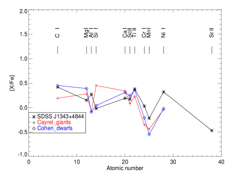
Figure 6: Elemental abundance for SDSS J1343+4844, compared with samples available from Cayrel et al. (2004) and Cohen et al. (2004). The red crosses indicate the mean elemental abundances from the Cayrel sample and the open diamonds represent the mean abundance values of the Cohen sample (EMP stars). The black asterisks represent the abundances of SDSS J1343+4844.

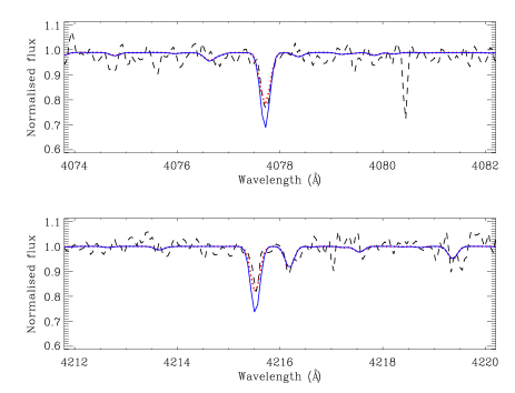
Figure 7: The Sr II lines at 4077 Å and 4216 Å are shown. The APO spectrum is plotted as a black dashed line, The abundance value derived from the equivalent-width analysis is used for the synthetic spectrum and plotted as a red dotted line. The blue solid line indicates the synthesized spectrum for [Sr/Fe] = 0.

6 Discussion and conclusions

6.1 CNO abundances in unevolved stars with [Fe/H] $<-3.0$

Metal-poor stars with enhanced/peculiar abundances in certain key elements help to identify the nuclear processes and astrophysical sites of their production. However, it is also interesting to study objects that do not exhibit such enhancements, since they may represent the mean ISM abundances at those epochs. This will help to understand the frequency of the nuclear sites that produce the peculiar abundance enhancements. SDSS J1343+4844 does not exhibit enhancement of C and possibly N and O abundances, indicating that there was no internal CN processing, which is consistent with its evolutionary stage as a subgiant. Spite et al. (2006) and Bonifacio et al. (2009) show that the mean [C/Fe] abundance ratios in unmixed giants and dwarfs are about [C/Fe] = +0.19 and [C/Fe] = +0.45, respectively. The SAGA compilation (Suda et al., 2008) and Figure 2 of Bonifacio et al. (2009) also show that the carbon abundance ratios in the carbon-normal EMP stars are slightly enhanced with respect to the solar ratio. SDSS J1343+4844 has [C/Fe] = $+$0.42, based on the low-resolution spectrum, consistent with these EMP stars.

6.2 Stars with low $\alpha$-element abundances at [Fe/H] $<-3.0$

In spite of having similar elemental abundances compared with the mean abundances of EMP stars, SDSS J1343+4844 belongs to the rare class of carbon-normal EMP stars that exhibit low $\alpha$-element abundances. It is thus interesting explore the origin of such stars.

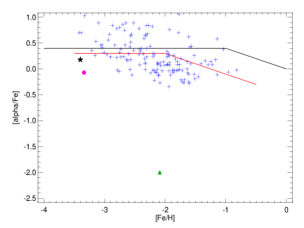
Figure 8: $\alpha$-elemental abundance for SDSS J1343+4844 (black star), compared with samples available from Ivans et al. (2003) (green filled triangle),Vargas et al. (2013) (the blue crosses),Caffau et al. (2013) (magenta filled circle). The black line is the schematic representation of the mean $\alpha$ abundance of the Milky Way halo, thick disk, and thin disk. The red line is a schematic representation of the mean $\alpha$ abundance of dwarf spheroidal galaxies.

Figure 8 shows the abundances of elements from the Vargas et al. (2013) sample. The $\alpha$-poor stars from Ivans et al. (2003) and Caffau et al. (2013) are also shown. SDSS J1343+4844 falls in the region close to the mean $\alpha$ abundances of dwarf galaxies. However the halo $\alpha$-element abudances for stars with [Fe/H] $<-3.0$ exhibit a large scatter.

Low $\alpha$-element abundances are expected for a low star-formation rate, similar to that found for many dwarf spheroidal galaxies. If this star belongs to a population that is representative of a low star-formation rate, inhomogeniously-mixed system, then SDSS J1343+4844 could be younger than other EMP stars, which are $\alpha$-element enhanced at the same metallicity.

6.3 Neutron-capture elements for stars with [Fe/H] $<-3.0$

SDSS J1343+4844 exhibits similar abundance patterns as those of EMP dwarfs and giants for the Fe-peak elements and n-capture elements as well. Strontium abundance ratios for EMP dwarfs and giants are between [Sr/Fe] = $-$0.6 and [Sr/Fe] = $-$0.1 at metallicities of [Fe/H] = $-3.0$ (Andrievsky et al., 2011), which is again similar to SDSS J1343+4844. The upper limit for the Ba abundance of our star ([Ba/Fe] $<-0.54$) lies well within the average Ba abundances of EMP stars having normal carbon abundance at the same metallicity (Cohen et al. 2013; [Ba/Fe] $\sim-0.6$).

During the early epochs of chemical evolution, asymptotic giant-branch stars would not have had time to contribute to the ISM (Kobayashi et al., 2014). They contribute significantly only after z = 1.8 (roughly [Fe/H] $>-$2.4). Hence, the n-capture elements seen in SDSS J1343+4844 have likely had contributions from massive stars. Recent observations of large opacity due to heavy elements in kilonovae Tanvir et al. (2013) has brought renewed interest in NS-NS mergers as a promising candidate for $r$-process-element production. NS-NS mergers were proposed long ago (Lattimer & Schramm, 1976; Lattimer et al., 1977; Meyer, 1989), and also in recent studies (Freiburghaus, Rosswog & Thielemann, 1999; Goriely, Bauswein & Janka, 2011; Rosswog et al., 2014; Wanajo et al., 2014; Vangioni et al., 2016), as promising sites for production of the $r$-process elements. Observationally-motivated work on this subject includes Honda et al. (2004), François et al. (2007), and Sneden, Cowan & Gallino (2008). These spectroscopic studies find a large scatter in [Eu/Fe] ratios (at least two orders of magnitude) for stars with [Fe/H] $\leq$ -2.5. They also show that the lighter and heavier $r$-process elements correlate very well, indicating possible connection, however their ratios at different metallicites suggest two possible evolutionary behaviours below [Fe/H] $<-2.5$. An additional mechanism, such as the LEPP (light element primary process), might be operating at metallicities [Fe/H] $<-3.0$ (Montes et al. 2007; Francois et al. 2007)

Most chemical evolution models are unable to explain all the observations. Recent work by Tsujimoto & Shigeyama (2014) and Ishimaru, Wanajo & Prantzos (2015) address these issues by assuming a chemical evolution of sub-halos with different masses and star-formation rates (SFR) contributing to the Galactic halo rather than chemical evolution within a single halo. Prantzos (2006) showed that if the sub-halos evolved at different rates, there would be no unique relation between age and metallicity; in that case there is possibility of an ”early” appearance of $r$-process elements and their large dispersion can be explained, even if the main source of those elements is NSMs.

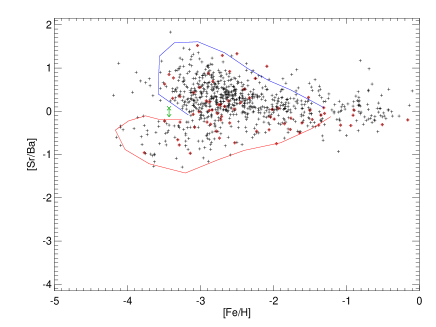
Figure 9: The evolution of lighter versus heavier $r$-process elemets are shown. The blue and red lines mark the contributions from massive and low-mass sub-halos that were accreted into the Galaxy, similar to Tsujimoto & Shigeyama (2015). The high ratios of [Sr/Ba] are due to massive sub-halos, while low [Sr/Ba] values are from low-mass sub-halos. These are non-CEMP stars, hence $s$-process contribution from stars with [Fe/H] $\leq-2.0$ is not expected. The data is from the SAGA database (Suda et al., 2008). SDSS J1343+4844 is marked as a green ’X’.

Figure 9 is motivated by Figure 2 in Tsujimoto & Shigeyama (2014). Tsujimoto & Shigeyama (2014) successfully explained the large scatter in [Eu/Fe] at low metallicities and the observed correlation between [light $r$-process/Eu] and [Eu/Fe]. According to these authors, CCSNe produce lighter $r$-process elements and the heavier $r$-process is produced by NS-NS mergers. The nucleosynthesis products of these two sources are mixed to different amounts within the sub-halos due to the differences in their wind speeds and a variations of sub-halo masses. A schematic diagram, shown in Figure 10, illustrates this. The high ratios of [light $r$-process/heavier $r$-process] is argued to be produced by massive sub-halos and a lower ratio is produced in low mass sub-halos.

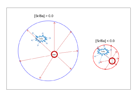
Figure 10: A schematic representation of the mechanism proposed by Tsujimoto & Shigeyama (2014). The wind from NS-MS mergers is shown in red and the wind from CCSNe are shown in blue. The wind from NS-NS mergers span the entire sub-halo, whereas the wind from CCSNe blast waves does not cover the entire massive sub-halo (10⁹M_⊙), but pollutes a larger filling factor for a low-mass halo (10⁶-10⁷M_⊙), producing different dilution and hence different ratios of [Sr/Ba].

Here we use barium to represent heavier $r$-process elements, and strontium to represent lighter $r$-process elements. The data shown in Figure 9 do not include carbon-enhanced stars, hence $s$-process contribution is not expected for stars with [Fe/H] $<-2.0$. The two regimes shown by Tsujimoto & Shigeyama (2014) are clearly seen in this figure as well. The region enclosed by the blue curve is expected to be occupied by stars that are formed within massive sub-halos (10⁹M_⊙) and the region enclosed by the red curve corresponds to stars that are formed within low-mass sub-halos (10⁶-10⁷M_⊙). SDSS J1343+4844 clearly falls in the middle of these distribution, indicating that the star is formed from a mixed ISM without peculiar composition. Figure 9 also shows the location of $\alpha$-poor stars with [$\alpha$/Fe] $<$ 0.1 (red dots). We find that they do not occupy any preferred location; rather, they are uniformly spread, in-spite of the two regions shown in the plot representing different mass ranges of the sub-halos. This result indicates that the SFRs for sub-halos of different masses may be similar during these epochs. Normally, $\alpha$-poor stars are expected to have formed in low-mass sub-halos with low SFRs. A different SFR for different sub-halo masses will also affect the [Sr/Ba] ratio, which does not match well with the observations. Apart from the sub-halo masses and SFR, the timescale of these sub-halos merging into the Galaxy is also essential for understanding the final abundance ratios.

6.4 Lithium depletion and binarity

The lithium line at 6707 Å is not detected in SDSS J1343+4844. The derived upper limit agrees with the declining lithium abundance trend for stars with [Fe/H] $<-3.0$ (Sbordone et al., 2010). There are two possibilities for the depletion of lithium: binary mass transfer and binary-induced mixing, or mixing due to the evolutionary status of the object as a subgiant. Detection of a radial-velocity variation with no peculiar chemical composition support the idea of binary-induced mixing. Most short-period binaries are found to have preserved their lithium, possibly due to tidal locking. However long-period binaries with periods of few hundred days seem to have depleted lithium abundances (Ryan & Deliyannis, 1995), which could be the case for SDSS J1343+4844.

6.5 Conclusions

We have derived LTE abundances for SDSS J1343+4844, a bright EMP star identified during the MARVELS pre-survey. The abundance pattern for most elements in this star are similar to other carbon-normal EMP stars, except for the low $\alpha$-element abundance and the apparent depletion of lithium. The depletion of lithium could be understood in terms of binary-induced mixing or additional convection, as the object is a subgiant. Low $\alpha$-element abundance, along with the agreement of the observed ratios of the carbon abundances and heavy elements with the mean EMP value is not so easy to understand. We also show that the $\alpha$-poor halo stars exhibit a wide range of lighter and heavier $r$-process ratios. An ISM with contributions from Pop III intermediate-mass stars, along with later Pop II contributions with a low SFR, may explain the abundance patterns seen in SDSS J1343+4844ṠDSS J1343+4844.

Predictions of several key elemental abundance ratios, especially C,N, $\alpha$ and light/heavy $r$-process elements from a chemical evolution model incorporating hierarchical merging of sub-halos of different masses and SFR may help to understand these observations.

6.6 acknowledgements

TCB acknowledges partial support for this work from grant PHY 14-30152; Physics Frontier Center/JINA Center for the Evolution of the Elements (JINA-CEE), awarded by the US National Science Foundation. The authors thank Thomas Masseron and Bertrand Plez for sharing the updated CH linelist. Many thanks to the referee, Chris Sneden, for his valuable inputs and willingness to discuss the paper before resubmission of the manuscript, which improved the paper considerably. SDSS-III MARVELS pre-survey data is used in this work. Funding for SDSS-III has been provided by the Alfred P. Sloan Foundation, the Participating Institutions, the National Science Foundation, and the U.S. Department of Energy Office of Science. The SDSS-III web site is http://www.sdss3.org/.

SDSS-III is managed by the Astrophysical Research Consortium for the Participating Institutions of the SDSS-III Collaboration including the University of Arizona, the Brazilian Participation Group, Brookhaven National Laboratory, Carnegie Mellon University, University of Florida, the French Participation Group, the German Participation Group, Harvard University, the Instituto de Astrofisica de Canarias, the Michigan State/Notre Dame/JINA Participation Group, Johns Hopkins University, Lawrence Berkeley National Laboratory, Max Planck Institute for Astrophysics, Max Planck Institute for Extraterrestrial Physics, New Mexico State University, New York University, Ohio State University, Pennsylvania State University, University of Portsmouth, Princeton University, the Spanish Participation Group, University of Tokyo, University of Utah, Vanderbilt University, University of Virginia, University of Washington, and Yale University.

Appendix

References

- Alonso, Arribas & Martinez-Roger (1996) Alonso A., Arribas S., Martinez-Roger C., 1996, A&A, 313, 873
- Alonso, Arribas & Martínez-Roger (1999) Alonso A., Arribas S., Martínez-Roger C., 1999, A&AS, 139, 335
- Alvarez & Plez (1998) Alvarez R., Plez B., 1998, A&A, 330, 1109
- Anderson, Zilitis & Sorokina (1967) Anderson E. M., Zilitis V. A., Sorokina E. S., 1967, Optics and Spectroscopy, 23, 102, (AZS)
- Andrievsky et al. (2011) Andrievsky S. M., Spite F., Korotin S. A., François P., Spite M., Bonifacio P., Cayrel R., Hill V., 2011, A&A, 530, A105
- Andrievsky et al. (2010) Andrievsky S. M., Spite M., Korotin S. A., Spite F., Bonifacio P., Cayrel R., François P., Hill V., 2010, A&A, 509, A88
- Aoki et al. (2009) Aoki W. et al., 2009, A&A, 502, 569
- Asplund (2005) Asplund M., 2005, ARA&A, 43, 481
- Barklem et al. (2005) Barklem P. S. et al., 2005, A&A, 439, 129
- Baumueller, Butler & Gehren (1998) Baumueller D., Butler K., Gehren T., 1998, A&A, 338, 637
- Baumueller & Gehren (1997) Baumueller D., Gehren T., 1997, A&A, 325, 1088
- Beers & Christlieb (2005) Beers T. C., Christlieb N., 2005, ARA&A, 43, 531
- Beers et al. (2014) Beers T. C., Norris J. E., Placco V. M., Lee Y. S., Rossi S., Carollo D., Masseron T., 2014, ApJ, 794, 58
- Bonifacio et al. (2009) Bonifacio P. et al., 2009, A&A, 501, 519
- Bromm, Yoshida & Hernquist (2003) Bromm V., Yoshida N., Hernquist L., 2003, ApJ, 596, L135
- Caffau et al. (2013) Caffau E. et al., 2013, A&A, 560, A15
- Carney et al. (1997) Carney B. W., Wright J. S., Sneden C., Laird J. B., Aguilar L. A., Latham D. W., 1997, AJ, 114, 363
- Castelli & Kurucz (2004) Castelli F., Kurucz R. L., 2004, ArXiv Astrophysics e-prints
- Cayrel et al. (2004) Cayrel R. et al., 2004, A&A, 416, 1117
- Cohen et al. (2004) Cohen J. G. et al., 2004, ApJ, 612, 1107
- Cohen et al. (2013) Cohen J. G., Christlieb N., Thompson I., McWilliam A., Shectman S., Reimers D., Wisotzki L., Kirby E., 2013, ApJ, 778, 56
- Cui, Sivarani & Christlieb (2013) Cui W. Y., Sivarani T., Christlieb N., 2013, A&A, 558, A36
- Cutri et al. (2003) Cutri R. M. et al., 2003, VizieR Online Data Catalog, 2246, 0
- Demarque et al. (2004) Demarque P., Woo J.-H., Kim Y.-C., Yi S. K., 2004, ApJS, 155, 667
- François et al. (2007) François P. et al., 2007, A&A, 476, 935
- Frebel & Norris (2015) Frebel A., Norris J. E., 2015, ARA&A, 53, 631
- Freiburghaus, Rosswog & Thielemann (1999) Freiburghaus C., Rosswog S., Thielemann F.-K., 1999, ApJ, 525, L121
- Ge et al. (2008) Ge J. et al., 2008, in Astronomical Society of the Pacific Conference Series, Vol. 398, Extreme Solar Systems, Fischer D., Rasio F. A., Thorsett S. E., Wolszczan A., eds., p. 449
- Goriely, Bauswein & Janka (2011) Goriely S., Bauswein A., Janka H.-T., 2011, ApJ, 738, L32
- Grevesse & Sauval (1998) Grevesse N., Sauval A. J., 1998, Space Sci. Rev., 85, 161
- Gunn et al. (2006) Gunn J. E. et al., 2006, AJ, 131, 2332
- Hansen, Montes & Arcones (2014) Hansen C. J., Montes F., Arcones A., 2014, ApJ, 797, 123
- Henden et al. (2015) Henden A. A., Levine S., Terrell D., Welch D. L., 2015, in American Astronomical Society Meeting Abstracts, Vol. 225, American Astronomical Society Meeting Abstracts, p. 336.16
- Honda et al. (2004) Honda S., Aoki W., Kajino T., Ando H., Beers T. C., Izumiura H., Sadakane K., Takada-Hidai M., 2004, ApJ, 607, 474
- Ishimaru, Wanajo & Prantzos (2015) Ishimaru Y., Wanajo S., Prantzos N., 2015, ApJ, 804, L35
- Ivans et al. (2003) Ivans I. I., Sneden C., James C. R., Preston G. W., Fulbright J. P., Höflich P. A., Carney B. W., Wheeler J. C., 2003, ApJ, 592, 906
- King (1997) King J. R., 1997, AJ, 113, 2302
- Kirby & Cohen (2012) Kirby E. N., Cohen J. G., 2012, AJ, 144, 168
- Kobayashi et al. (2014) Kobayashi C., Ishigaki M. N., Tominaga N., Nomoto K., 2014, ApJ, 785, L5
- Kobayashi et al. (2006) Kobayashi C., Umeda H., Nomoto K., Tominaga N., Ohkubo T., 2006, ApJ, 653, 1145
- Kurucz (2007) Kurucz R. L., 2007, Robert l. kurucz on-line database of observed and predicted atomic transitions
- Kurucz (2009) Kurucz R. L., 2009, Robert l. kurucz on-line database of observed and predicted atomic transitions
- Kurucz (2013) Kurucz R. L., 2013, Robert l. kurucz on-line database of observed and predicted atomic transitions
- Lai et al. (2008) Lai D. K., Bolte M., Johnson J. A., Lucatello S., Heger A., Woosley S. E., 2008, ApJ, 681, 1524
- Lai et al. (2009) Lai D. K., Rockosi C. M., Bolte M., Johnson J. A., Beers T. C., Lee Y. S., Allende Prieto C., Yanny B., 2009, ApJ, 697, L63
- Lattimer et al. (1977) Lattimer J. M., Mackie F., Ravenhall D. G., Schramm D. N., 1977, ApJ, 213, 225
- Lattimer & Schramm (1976) Lattimer J. M., Schramm D. N., 1976, ApJ, 210, 549
- Lee et al. (2008) Lee Y. S. et al., 2008, AJ, 136, 2050
- Martin, Fuhr & Wiese (1988) Martin G., Fuhr J., Wiese W., 1988, J. Phys. Chem. Ref. Data Suppl., 17
- Mashonkina, Korn & Przybilla (2007) Mashonkina L., Korn A. J., Przybilla N., 2007, A&A, 461, 261
- McWilliam et al. (1995) McWilliam A., Preston G. W., Sneden C., Searle L., 1995, AJ, 109, 2757
- Meyer (1989) Meyer B. S., 1989, ApJ, 343, 254
- Montes et al. (2007) Montes F. et al., 2007, ApJ, 671, 1685
- Otsuki et al. (2006) Otsuki K., Honda S., Aoki W., Kajino T., Mathews G. J., 2006, ApJ, 641, L117
- Plez (2012) Plez B., 2012, Turbospectrum: Code for spectral synthesis. Astrophysics Source Code Library
- Prantzos (2006) Prantzos N., 2006, ArXiv Astrophysics e-prints
- Roederer et al. (2012) Roederer I. U. et al., 2012, New Hubble Space Telescope Observations of Heavy Elements in Four Metal-Poor Stars
- Roederer et al. (2014) Roederer I. U., Preston G. W., Thompson I. B., Shectman S. A., Sneden C., Burley G. S., Kelson D. D., 2014, AJ, 147, 136
- Rosswog et al. (2014) Rosswog S., Korobkin O., Arcones A., Thielemann F.-K., Piran T., 2014, MNRAS, 439, 744
- Ryan & Deliyannis (1995) Ryan S. G., Deliyannis C. P., 1995, ApJ, 453, 819
- Sbordone et al. (2010) Sbordone L. et al., 2010, A&A, 522, A26
- Schlegel, Finkbeiner & Davis (1998) Schlegel D. J., Finkbeiner D. P., Davis M., 1998, ApJ, 500, 525
- Smith & Liszt (1971) Smith W. H., Liszt H. S., 1971, Journal of the Optical Society of America (1917-1983), 61, 938, (SLa)
- Sneden, Cowan & Gallino (2008) Sneden C., Cowan J. J., Gallino R., 2008, ARA&A, 46, 241
- Sobeck, Lawler & Sneden (2007) Sobeck J. S., Lawler J. E., Sneden C., 2007, ApJ, 667, 1267
- Spite et al. (2012) Spite M. et al., 2012, A&A, 541, A143
- Spite et al. (2006) Spite M. et al., 2006, A&A, 455, 291
- Suda et al. (2008) Suda T. et al., 2008, PASJ, 60, 1159
- Tafelmeyer et al. (2010) Tafelmeyer M. et al., 2010, A&A, 524, A58
- Tanvir et al. (2013) Tanvir N. R., Levan A. J., Fruchter A. S., Hjorth J., Hounsell R. A., Wiersema K., Tunnicliffe R. L., 2013, Nature, 500, 547
- Tsujimoto & Shigeyama (2014) Tsujimoto T., Shigeyama T., 2014, ApJ, 795, L18
- Vangioni et al. (2016) Vangioni E., Goriely S., Daigne F., François P., Belczynski K., 2016, MNRAS, 455, 17
- Vargas et al. (2013) Vargas L. C., Geha M., Kirby E. N., Simon J. D., 2013, ApJ, 767, 134
- Wanajo et al. (2014) Wanajo S., Sekiguchi Y., Nishimura N., Kiuchi K., Kyutoku K., Shibata M., 2014, ApJ, 789, L39
- Wiese, Smith & Glennon (1966) Wiese W. L., Smith M. W., Glennon B. M., 1966, Atomic transition probabilities. Vol.: Hydrogen through Neon. A critical data compilation, Wiese, W. L., Smith, M. W., & Glennon, B. M., ed. US Government Printing Office, (WSG)
- Wood et al. (2013) Wood M. P., Lawler J. E., Sneden C., Cowan J. J., 2013, ApJS, 208, 27
- Wood et al. (2014) Wood M. P., Lawler J. E., Sneden C., Cowan J. J., 2014, ApJS, 211, 20
- Wright et al. (2010) Wright E. L. et al., 2010, AJ, 140, 1868
- Wright & Howard (2009) Wright J. T., Howard A. W., 2009, ApJS, 182, 205
- Yong et al. (2013) Yong D. et al., 2013, ApJ, 762, 26