Blocking temperature of interacting magnetic nanoparticles with uniaxial and cubic anisotropies from Monte Carlo simulations.

Abstract

The low temperature behavior of densely packed interacting spherical single domain nanoparticles (MNP) is investigated by Monte Carlo simulations in the framework of an effective one spin model. The particles are distributed through a hard sphere like distribution with periodic boundary conditions and interact through the dipole dipole interaction (DDI) with an anisotropy energy including both cubic and uniaxial symmetry components. The cubic component is shown to play a sizable role on the value of the blocking temperature $T_{b}$ only when the MNP easy axes are parallel to the cubic easy direction ([111] direction for a negative cubic anisotropy constant). The nature of the collective low temperature state, either ferromagnetic or spin glass like, is found to depend on the ratio of the anisotropy to the dipolar energies characterizing partly the disorder in the system.
Keywords : Magnetic nanoparticles; Blocking temperature; Monte Carlo simulations.

I Introduction

Magnetic nanoparticles still arouse a great interest both on the fundamental point of view in nanomagnetism Skomski (2003); Majetich and Sachan (2006); Skomski (2008); Bedanta and Kleemann (2009); Bedanta et al. (2013) and in the field of applications especially in nanomedecine Pankhurst et al. (2003, 2009); Owen et al. (2012). Under a critical radius $r_{sd}$ depending on their chemical composition, determined by the ratio of the energy necessary to sustain a domain wall to the magnetostatic energy, magnetic nanoparticles (MNP) are single domain objects (see for instance Dormann et al. (1997); Skomski (2003)). Typical values for $r_{sd}$ are 15 nm for Fe, 35 nm for Co, 30 nm for $\gamma$-Fe₂O₃ Dormann et al. (1997); Bedanta and Kleemann (2009). Under this critical size, the simplification due to the single domain character leads to the effective one spin (or macrospins) models where the MNP are represented as uniformly magnetized particles. As a consequence, the anisotropy energy is to be understood as an effective one, since no direct reference to crystalline defects and to spin canting can be considered, and includes contributions stemming from the MNP shape, crystalline anisotropy or surface effects. Although the local stucture of the MNP is then frozen, such effective one spin models (EOS) have shown to give results in agreement with experiments Russier et al. (2012). In most cases the MNP are coated by a non magnetic layer making them exchange uncoupled. As a result, the theoretical description of single domain magnetic nanoparticles assemblies faces mainly two difficulties: the long range nature of the dipolar interactions and the one body magneto-crystalline anisotropy energy (MAE). The former is at the origin of collective behavior Bedanta and Kleemann (2009); Bedanta et al. (2013) at low temperature while the later leads to irreversibility, namely the so-called blocking phenomenon and hysteresis Dormann et al. (1997). Both the inter-particle interactions and the individual anisotropy influence the magnetic properties of the assemblies with different kind of signature, the former being essentially dependent on the underlying structure while the later characterizes only the individual MNP. The importance of the dipole dipole interactions (DDI), for a given value of the MNP moment, namely for a given material and mean value of the diameter, is controlled by the inter-particle distances, via the MNP concentration in the assembly. In addition, the nature of the state induced at low temperature by the collective behavior resulting from the DDI depends strongly on the underlying structure and dimensionality because of the anisotropic character of the dipolar interaction. It can be in principle ferromagnetic or anti–ferromagnetic for sufficiently ordered or concentrated systems Wei and G.N. (1992); Weis and Levesque (1993); Weis (2005), or spin–glass like (SSG) Ayton et al. (1997); Petracic (2010); Bedanta et al. (2013) for more disordered ones as has been evidenced experimentally Petracic et al. (2006); Parker et al. (2007); Wandersman et al. (2008); Nakamae (2014); Mohapatra et al. (2015). We emphasize that the degree of structural disorder is of crucial importance on this point and that this latter can be partly induced and/or modified by the MAE according to both its magnitude and the corresponding easy axes distribution. On an other hand, the magnitude and the symmetry of the anisotropy terms depend on the crystalline nature of the material, the actual size, shape and surface characteristics of the MNP Coey (2010); Bedanta and Kleemann (2009). It is worth mentioning that the influence of both the DDI and the MAE on the magnetic properties are strongly temperature dependent: indeed, the MAE induced irresversibility behavior is expected below the blocking temperature, while the influence of the MAE on the room temperature magnetization curve is quite important only at sufficiently large values of the applied field Margaris et al. (2012); Russier et al. (2013). Concerning the MAE an important issue is the interplay between cubic and uniaxial symmetries Usov and Peschany (1997); Geshev et al. (1999); Margaris et al. (2012); Sabsabi et al. (2013); Russier et al. (2013); Usov and Barandiarán (2012); M.J.Correia et al. (2014). This has been studied in detail essentially for assemblies of non interacting Usov and Barandiarán (2012); M.J.Correia et al. (2014) or weakly interacting particles Margaris et al. (2012); Sabsabi et al. (2013). In the strong DDI coupling, corresponding to concentrated dried powders of MNP this topic has been addressed for the magnetization curve at room temperature Russier et al. (2013). One of the motivations of Refs. Usov and Barandiarán (2012); Russier et al. (2013) was to examine the possibility to get evidence of a cubic component in the MAE from an experimentally observable property, a goal motivated by the usual experimental determination of the anisotropy constant from the blocking temperature once the MNP size is known through a Stoner-Wohlfarth relaxation law. Following this procedure, one assumes a priori a uniaxial symmetry for the MAE while a large fraction of works on MNP refer to particles made of materials with cubic symmetry, as for instance the cubic spinel ferrites. Then the uniaxial symmetry term can result from either the shape or surface contribution Skomski (2003) but nevertheless the bulk cubic contribution cannot be simply ignored. Quite interestingly, Garanin and Kachkachi Garanin and Kachkachi (2003) and Kachkachi and Bonnet Kachkachi and Bonet (2006) have shown that the surface anisotropy, when modeled from the Néel surface anisotropy model Néel (1954), can be represented by a cubic contribution to the total MAE leading to an effective one spin model which strengthens the usefulness of the combined symmetries MAE study. In Refs. Soler et al. (2012); Neumann et al. (2013) Monte Carlo simulations of magnetic properties including the blocking temperature of thin films composed of $\gamma$-Fe₂O₃ NP embedded in polyaniline have been performed with NP interacting through DDI and characterized by two MAE terms of uniaxial symmetry, stemming from shape and crystalline anisotropy respectively.

In the present work we focus on the effect of combined anisotropies of uniaxial and cubic symmetries. Conversely to the preceding paper, where the equilibrium magnetization was concerned, we consider the blocking temperature as determined from the so-called ZFC/FC curves. As in our previous work Russier et al. (2013), we deal with concentrated systems with high dipolar coupling and we deal only with MNP assemblies fixed in position where the underlying structure is determined from a hard sphere like distribution. A particular attention is paid on the nature of the frozen orientational state reached at low temperature, and we show the influence of the MAE induced disorder on this point.

II Model

We model the assembly of spherical single domain MNP in the framework of macro spin model. We neglect the size polydispersity and so consider an assembly of dipolar hard spheres uniformly polarized with magnetization $M_{s}$ and diameter $d$. The uniaxial and cubic components of the magneto-crystalline anisotropy, described by the corresponding single site interactions on the moment orientations, $\hat{m}_{i}$ (see equation (II)) are characterized on the first hand by the anisotropy constants $K_{u}$ and $K_{c}$ and on the other hand by the uniaxial $\{\hat{n}\}_{i}$ and the cubic $\{\hat{x}_{\alpha\;=\;1,3}\}_{i}$ easy axes respectively. The distance of closest approach between MNP, say $d_{eff}\;=\;d\;+\;\Delta$, may differ from $d$ due to a non magnetic coating layer of thickness $\Delta/2$ surrounding the MNP. We focus on an assembly of MNP in a frozen disordered state. The structure of the assembly is modeled by a true hard sphere configuration, say $\bm{R}\;=\{\vec{r}_{i}\}$, obtained by a Monte Carlo evolution of hard sphere particles starting from a face centered cubic (fcc) lattice at a fixed density. The resulting distribution is controlled through the radial distribution function $g_{hs}(r)$ and more precisely the contact value, $g_{hs}(d_{eff})$, related the hard sphere fluid pressure Hansen and McDonald (2006). The hard sphere system thus defined is totally characterized by the volume fraction $\Phi$ = $(\pi/6)\rho{}d_{eff}^{3}$ where $\rho$ is the number of particles per unit volume. We also introduce the MNP volume fraction, $\Phi_{p}$ = $\Phi(d/d_{eff})^{3}$. The particles are then fixed in position. Periodic boundary conditions are used throughout the paper. The total energy of the system which includes the (DDI), the uniaxial and the cubic contributions to the anisotropy energy (MAE) and the Zeeman energy respectively

$$E=E_{dd}+E_{u}+E_{c}+E_{z}$$ (1)

is given, in reduced form after introducing a reference inverse temperature, $\beta_{0}$ = $1/(k_{B}T_{0})$, by

$$\beta_{0}E = \epsilon_{d}\sum_{i<j}\frac{\hat{m}_{i}\hat{m}_{j}-3(\hat{m}_{i}\hat{r}_{ij})(\hat{m}_{j}\hat{r}_{ij})}{r_{ij}^{*3}}-\epsilon_{u}\sum_{i}(\hat{n}_{i}\hat{m}_{i})^{2}-\frac{\epsilon_{c}}{2}\sum_{i}\sum_{\alpha}(\hat{m}_{i}\hat{x}_{\alpha i})^{4}-h\sum_{i}\hat{m}_{i}\hat{h}\leavevmode\nobreak\ .$$

with the coupling constants and the reduced external field,

$$\epsilon_{u} = \beta_{0}K_{u}v(d)\leavevmode\nobreak\ ;\leavevmode\nobreak\ \epsilon_{c}=\beta_{0}K_{c}v(d)$$

$$\epsilon_{d} = \frac{\beta_{0}\mu_{0}}{4\pi}(\pi/6)M_{s}^{2}v(d)(d/d_{eff})^{3}\leavevmode\nobreak\ \equiv\leavevmode\nobreak\ \epsilon_{d}^{(0)}(d/d_{eff})^{3}\leavevmode\nobreak\ \leavevmode\nobreak\ ;\leavevmode\nobreak\ \leavevmode\nobreak\ h=\beta_{0}\mu_{0}M_{s}v(d)H_{a}\leavevmode\nobreak\ \equiv\leavevmode\nobreak\ {H_{a}}{H_{ref}}$$

The long ranged dipolar interactions (DDI) are treated in the framework of the Ewald summation technique Allen and Tildesley (1987); Frenkel and Smit (2002) and the total expression including the latter can be found for instance in Ref. Weis and Levesque (1993). In equations (II, II) hatted letters represent unit vectors, $r_{ij}^{*}=r_{ij}/d_{eff}$ and $v(d)=(\pi/6)d^{3}$ is the MNP volume. We also introduce the reduced temperature, $T^{*}\;=\;T/T_{0}$. Since we have in mind to model systems where no texturation is expected, such as powders or random close packed samples, we consider the MNP as randomly oriented one to each other. Accordingly the cubic contribution, a priori related to the crystallographic orientations of the MNP’s considered as nano crytallites (NC), is characterized by randomly distributed set of axes $\{\hat{x}_{\alpha}\}_{i}$. On the other hand, as in Ref. Russier et al. (2013) the uniaxial easy axes are also randomly distributed but are either uncorrelated with or fixed to a given crystallographic orientation of the NC. In this later case, we consider the situation of uniaxial and cubic contributions acting in a constructing way. With a negative cubic anisotropy constant used throughout this work, the usual case for cubic spinel ferrites, this means uniaxial easy axes in the $[111]$ direction of the NC. A similar situation is obtained with $k_{c}\;>\;0$ and uniaxial easy axes parallel to one of the cubic easy axes, namely $\hat{n}_{i}\;=\;\hat{x}_{i}$ (equivalently $\hat{y}_{i}$ or $\hat{z}_{i}$).

The determination of the blocking temperature is performed from the so-called FC/ZFC magnetization curves which we simulate from Monte Carlo runs including at each temperature step 2.5 10⁴ Monte Carlo steps (MCS) the last 1.25 10⁴ of which are used to perform the thermal averages. The ZFC curves are initiated from a true demagnetized low temperature state, which is obtained from a long Monte Carlo run, up to 2 10⁵ MCS performed using a parallel tempering scheme Hukushima and Nemoto (1996) to overcome the expected slowing down behavior due to the strong dipolar coupling regime as well as the deep MAE potential wells. Each ZFC and FC magnetization curve is determined from the average on a set (up to 48) of independent MC paths performed using either one or several different structural configurations (hard sphere distributions) This is is necessary in order to get an average over disorder, see equation (5), due to both the random character of the easy axes distribution and the underlying hard sphere like structure. This procedure is performed using a parallel code where the paths are run simultaneously and the corresponding averages are calculated as a final step.

On an other hand, since we deal with concentrated system with a high dipolar coupling, we expect the dipolar particles to present a collective state which may be of ferro magnetic or spin glass character. To discriminate from these possibilities we examine, at zero external field, the spontaneous magnetization and the nematic order parameter $\lambda$ defined as the largest eigenvalue of the second rank tensor Levesque and J.-J.Weis (1994)

$$\bar{Q}=\frac{1}{N}\sum_{i}\frac{1}{2}(3\hat{m}_{i}\hat{m}_{i}-\bar{I})\leavevmode\nobreak\ ,$$ (4)

where $\bar{I}$ is the unit tensor. This is done as usual by using the so-called conductive external conditions which prevent the occurrence of demagnetizing effect Allen and Tildesley (1987); Weis and Levesque (1993). Such external conditions remain to consider the simulated system as immersed in an external medium of infinite permeability. For the simulation of the spontaneous magnetization, we also use the parallel tempering scheme to avoid the important slowing down of the relaxation in the system related to the occurrence of the frozen collective state. The spontaneous magnetization $<M>$ is determined from the average of thermal statistical mean values, $<M(\bm{R}_{n})>_{T}$ over a set of different hard sphere configurations $\bm{R}_{n}$ Klapp and Patey (2001), namely

$$<M>\leavevmode\nobreak\ =\frac{1}{N_{R}}\sum_{n=1}^{N_{R}}<M(\bm{R_{n}})>_{T}.$$ (5)

III Results

In this work we do not aim to simulate a specific experimental system; instead we focus on the qualitative trend expected for typical magnetic MNP with iron oxides as a guide for the choice of the physical parameters, because of their importance in the field and the representativity of their physical properties ($K_{c}$ or $M_{s}$), in the family of oxide spinel ferrites excepted CoFe₂O₄. Since these materials present a cubic structure, we estimate the MAE uniaxial component from the shape anisotropy, assuming an aspect ratio of say $\delta$ $\simeq$ 1.10 to 1.20. Starting from $\mu_{0}M_{s}$ = 0.5 T and $K_{c}$ = -13 kJm^-3 (-4.7 kJm^-3), the room temperature values of the cubic anisotropic constant for magnetite (maghemite), and setting $T_{0}$ to the room temperature we get a bare dipolar coupling constant ranging from $\epsilon_{d}^{(0)}$ = 1 to 8.0, $\left|\epsilon_{c}\right|$ $\simeq$ 1.65 (0.60) to 8.10 (2.95) and $\epsilon_{u}$ $\sim$ 0.5 to $\sim$ 7.25 for MNP with diameter in between $d$ = 10 nm to 20 nm. This corresponds to the range of validity of the macro spin models since they are limited to MNP whose radius is on the one hand larger than some threshold value, say $\sim$ 2 nm Dormann et al. (1997), under which the majority of atoms lie in the surface and on the other hand smaller than the single domain critical size $r_{sd}$ recalled in the introduction. In the following the parameters retained for the simulations are taken within the above ranges of values. We limit the DDI coupling to $\epsilon_{d}\;\leqslant\;2$ which, for instance, corresponds to include a coating layer $\Delta/2\;=\;2\;nm$ on magnetite MNP of $d$ = 16 $nm$ in diameter. Since we expect, from results obtained in the superparamagnetic regime Russier et al. (2013), that the cubic contribution leads to a sizable effect only when $\left|\epsilon_{c}\right|\;>\;3\;\epsilon_{u}$ at least in the presence of DDI we limit our simulations to $\left|\epsilon_{c}\right|\;=\;4\;\epsilon_{u}$. All the simulations are performed for a dense system characterized by $\Phi$ = 0.493 ($\phi_{p}\;\simeq\;0.250$ if we include a coating layer $\Delta/2\;\simeq\;d/8.0$) with $N_{p}$ = 1728 particles in the simulation box.

$\epsilon_{d}$	$\epsilon_{u}$	$\epsilon_{c}$	$\hat{n}_{u}$	Tb
0.0	2.00	0.00		0.218
0.0	2.00	-8.00	rand	0.270
0.0	2.00	-8.00	[111]	0.304
1.0	0.60	0.00		0.257
1.0	2.00	0.00		0.400
1.0	2.00	-8.00	rand	0.410
1.0	2.00	-8.00	[111]	0.510
1.0	3.40	0.00		0.580
2.0	1.40	0.00		0.557
2.0	2.00	0.00		0.643
2.0	2.00	-8.00	rand	0.659
2.0	2.00	-8.00	[111]	0.735
2.0	3.40	0.00		0.693

Table 1: Blocking temperature in terms of the coupling constants of the model.

Let us recall that the cubic axes ($\{\hat{x}_{\alpha}\}_{i}$) are randomly distributed and we limit ourselves to two different situations: the uniaxial easy axes are either uncorrelated to the cubic ones or are fixed in the referential of the later in such a way to maximize the global anisotropy effect, namely coincide with the [111] direction of the local frame, $\hat{n}_{i}\;=\;(\sum_{\alpha}\hat{x}_{\alpha{i}})/\sqrt{3}$ for $\epsilon_{c}\;<\;0$. This will be referred to in the following as random or [111] easy axes distributions respectively, implicitly referring to the local referential of the MNP. According to our preceding results, we expect comparable results for $k_{c}\;<\;0$ and $\hat{n}_{i}$ = [111]_i and for $k_{c}\;>\;0$ with $\hat{n}_{i}$ = $\hat{x}_{i}$, considered in Ref. M.J.Correia et al. (2014) for non interacting MNP.

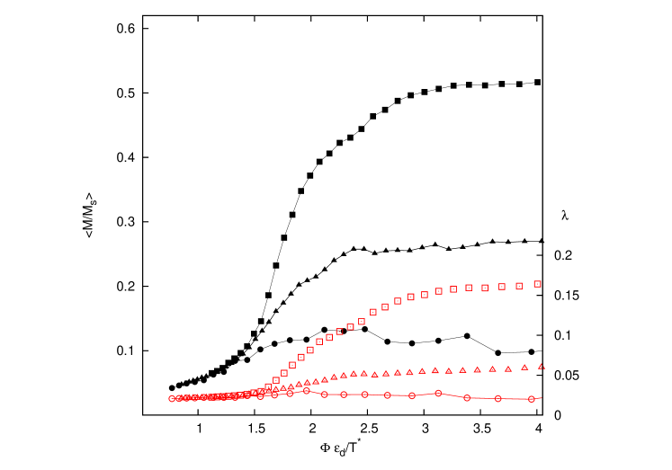
Figure 4: Spontaneous polarization, left hand scale and solid symbols, and nematic order parameter $\lambda$, right hand scale and open symbols, in terms of $\epsilon_{d}/T^{*}$. Periodic boudary conditions with conducting external conditions. $\epsilon_{c}$ = 0. Squares: $\epsilon_{u}$ = 0; triangles: $\epsilon_{d}$ = 1.0 and $\epsilon_{u}$ = 0.60; circles: $\epsilon_{d}$ = 2.0 and $\epsilon_{u}$ = 2.0.

The results obtained for the blocking temperature are given in table 1 and in figure (1). First of all, we confirm the well known increase of $T_{b}$ with the DDI García-Otero et al. (2000); Vargas et al. (2005). The corresponding FC/ZFC curves are displayed in figures (2) and (3) in the absence of cubic anisotropy for non interacting and interacting MNP, with $\epsilon_{d}$ = 1.0, respectively. The plateau like behavior of the FC magnetization curve at $T\;<\;T_{b}$, known to result from the collective behavior induced by the DDI is clearly seen. At the qualitative level, the FC magnetization curves displayed in figure (3) are quite similar, the main difference being the value taken by $T_{b}$; nevertheless we note that when the MAE coupling constant takes a rather small value, $\epsilon_{u}$ = 0.60 and 1.40 for $\epsilon_{d}$ = 1 and 2 respectively, i.e. $\epsilon_{u}/\epsilon_{d}\;\leqslant\;0.70$, the FC magnetization for $T\;<\;T_{b}$ still increases slightly when $T$ decreases, while for higher values corresponding to $\epsilon_{u}/\epsilon_{d}\;\geq\;1$, the FC curves present first a true plateau with possibly a small dip. The latter behavior is known as the signature of a super spin glass state De-Toro et al. (2013); Petracic et al. (2006); Parker et al. (2007); Nakamae (2014). Therefore, we are lead to conclude that when the ratio $\epsilon_{u}/\epsilon_{d}$ increases beyond a threshold value $\epsilon_{u}/\epsilon_{d}$ = $k_{s}$ $\sim$ 0.6, a super spin glass state is reached at low temperature while, when $\epsilon_{u}/\epsilon_{d}\;<\;k_{s}$ the low temperature collective state may be closer to a ferromagnetic state expected for $\epsilon_{u}$ = 0 at least in the monodisperse case and for the high value of the volume fraction used here Klapp and Patey (2001); Ayton et al. (1997). Since the easy axes are randomly distributed the ratio $\epsilon_{u}/\epsilon_{d}$ measures the degree of disorder introduced in the system in addition to the structural one resulting from the hard sphere like MNP distribution and thus is expected to bring the system from the ordered ferromagnetic phase to the disordered super spin glass one. Although the precise determination of the nature of the collective state at low temperature is beyond the scope of the present paper, we strengthen the above interpretation from the calculation of the spontaneous magnetization and of the nematic order parameter at zero field, given by equation (4). The result is displayed in figure (4) for $\epsilon_{u}/\epsilon_{d}$ = 0, 0.6 and 1.0 in terms of the relevant variable ($\Phi\epsilon_{d}/T^{*}$). The spontaneous magnetization curves versus $\Phi\epsilon_{d}/T^{*}$ in the cases $\epsilon_{d}$ = 1, $\epsilon_{u}$ = 0.6 and $\epsilon_{d}$ = 2, $\epsilon_{u}$ = 1.4 respectively are very similar. We see that in the absence of anisotropy a clear ferromagnetic phase is reached, while for $\epsilon_{u}/\epsilon_{d}$ = 0.6, although the spontaneous magnetization does not vanish, $\lambda$ takes a quite small value and no clear jump is obtained conversely to the $\epsilon_{u}$ = 0 case. It is worth recalling that pure dipolar hard spheres ($\epsilon_{u}\;=\;\epsilon_{c}\;=\;0$) located at the nodes of a well ordered cfc lattice, present a ferromagnetic phase characterized by both $<M/M_{s}>\;\rightarrow\;1$ and $\lambda\;\rightarrow\;1$ when $T^{*}\;\rightarrow\;0$ Weis and Levesque (1993); Weis (2005) and, more precisely, to compare with the results displayed in figure (4) we get $<M/M_{s}>\;=\;0.91$ and $\lambda\;=\;0.75$ for ($\Phi\epsilon_{d}/T^{*}$) = 4 Russier (2015). The spontaneously magnetized phase at zero field we get for $\epsilon_{u}$ = 0 is comparable to the disordered ferromagnetic phase obtained in Klapp and Patey (2001) on a quite similar system. We have checked from simulations with 864 or 2048 particles that in this later case, $<M>$ and $\lambda$ depend only very weakly on the system size, which shows that we are not dealing with a large but finite cluster ferromagnetically correlated. Then either for $\epsilon_{u}/\epsilon_{d}\;>\;0.7$ with $\epsilon_{c}$ = 0 or in general $\epsilon_{u}\;\neq\;0$ and $\epsilon_{c}\;\neq\;0$ both the spontaneous magnetization and $\lambda$ vanish.

The effect of the MAE cubic contribution on $T_{b}$ depends strongly on the relative orientation of the uniaxial and cubic easy axes. When the uniaxial easy axes are uncorrelated to the cubic ones, the deviation of $T_{b}$ due to the cubic term is very small for MNP interacting through DDI and is small but nevertheless significant in the non interacting case, as can be seen in table 1 and on figure 1 and 5. This is in agreement with what is found in the superparamagnetic regime for the behavior of the magnetization curve in the intermediate external field range Russier et al. (2013). When the uniaxial easy axes $\{\hat{n}\}_{i}$ are set parallel to the [111] direction of the local MNP frames, the cubic contribution to the MAE has a sizable effect on $T_{b}$ both for non interacting and interacting MNP. The deviation $(T_{b}^{*}(\epsilon_{c})\leavevmode\nobreak\ -\leavevmode\nobreak\ T_{b}(0))$ is then found nearly independent of $\epsilon_{d}$ which corresponds to a relative weakening of the influence of $\epsilon_{c}$ when $\epsilon_{d}$ is increased. Indeed, still for $\{\hat{n}\}_{i}$ set parallel to the MNP [111] direction, if we consider $T_{b}$ in terms of the ratio $\left|\epsilon_{c}\right|/\epsilon_{u}$ as is done in the non interacting case by Correia et al. M.J.Correia et al. (2014), we get from our simulations $T_{b}(\left|\epsilon_{c}\right|/\epsilon_{u}\leavevmode\nobreak\ =\leavevmode\nobreak\ 4)/T_{b}(0)$ = 1.39, 1.26 and 1.14 for $\epsilon_{d}$ = 0, 1 and 2 respectively. Notice that the result for the latter ratio in the non interacting case ($\epsilon_{d}$ = 0) is very close to what Correia et al. have obtained M.J.Correia et al. (2014) although the $T_{b}$ values are not strictly comparable since $T_{b}$ depend on the simulation ’time’ and moreover, Ref. M.J.Correia et al. (2014) correspond to the easy axes in the [001] direction with $\epsilon_{c}\;>\;0$. The behavior of $T_{b}$ with respect to the cubic component in either the [111] or the random uniaxial easy axes distribution, obtained in the present work (see Table 1 and Fig. 5), is in agreement with that of the hysteresis curves calculated by Usov and Barandiarán Usov and Barandiarán (2012) in the sense that we show that both a strong cubic to uniaxial energies ratio and conveniently correlated orientations of the two symmetries easy axes is necessary for the cubic MAE contribution to significantly influence $T_{b}$. The low temperature plateau of the FC magnetization curve is much more marked when the MAE cubic contribution does not vanish and especially for the [111] easy axes distribution. Moreover, at low temperature ($\Phi\epsilon_{d}/T^{*}\;>\;4$), both the spontaneous magnetization and the nematic order parameter vanish when $\epsilon_{c}\;\neq\;0$.

Finally we compare the FC/ZFC and the resulting $T_{b}$ in the pure uniaxial or cubic cases with comparable individual barrier heights. This is done by noting that the uniaxial MAE barrier height is $\epsilon_{u}$ while the cubic MAE one is given by $-\epsilon_{c}/12$ with $\epsilon_{c}\;<\;0$ since the moment must go through the saddle point in the [110] direction in order to jump from one [111] potential well to an other one. Therefore we compare as an example the cases ($\epsilon_{u}$ = 2, $\epsilon_{c}$ = 0) with ($\epsilon_{u}$ = 0, $\epsilon_{c}$ = -24) and ($\epsilon_{u}$ = 1.40, $\epsilon_{c}$ = 0) with ($\epsilon_{u}$ = 0, $\epsilon_{c}$ = -16.8) for $\epsilon_{d}$ = 0 and 2 respectively where we get $T_{b}$ = 0.22 and 0.29 on the first hand and $T_{b}$ = 0.56 and 0.58 respectively. Only in the non interacting case the corresponding pure cubic $T_{b}$ values is significantly larger than the pure uniaxial one, while a quasi coincidence is obtained for $\epsilon_{d}\leavevmode\nobreak\ \neq$ 0. This is in agreement with the relative weakening due to the DDI of the $\epsilon_{c}$ contribution to $T_{b}$.

To conclude, in this work first of all we confirm at low temperature the results we obtained on large spherical clusters in the superparamagnetic regime, concerning the influence of the MAE cubic contribution. This contribution to the magnetization behavior is significant only when the MNP easy axis is locally fixed to the relevant MNP local orientation ([111] or [100] for $\epsilon_{c}$ $<$ 0 or $>$ 0 respectively) and the corresponding deviation in $T_{b}$ is found nearly independent of $\epsilon_{d}$. We also characterize at least at the qualitative level the nature of the frozen low temperature phase, which is found to present either a ferromagnetic or a spin-glass character depending on the value taken by the ratio $\epsilon_{u}/\epsilon_{d}$ contributing to the degree of disorder in the system for randomly distributed easy axes. Conversely to our preceding work we consider only periodic boundary conditions and a true hard sphere distribution is used for the MNP structure with the limitation to the monodisperse case.

IV Acknowledgements

We acknowledge very useful discussions with Dr. J.J.- Weis from the LPT, UMR 8627 of CNRS and Université Paris-Sud, Dr. I. Lisiecki and Dr. J. Richardi from the MONARIS, UMR 8233 of CNRS and Université UPMC and Dr. S. Nakamae from the SPEC, UMR 2464 of CEA and CNRS. This work was granted access to the HPC resources of CINES under the allocation 2015-096180 made by GENCI. We acknowledge financial support from the French research agency ANR grant ANR-CE08-007 for part of the calculations performed in this work.

Figure 1: Blocking temperature dependence on the dipolar interaction strength $\epsilon_{d}$, for $\epsilon_{u}$ = 2; $\epsilon_{c}$ = 0 (squares); $\epsilon_{c}$ = -8 and $\hat{n}$ uncorrelated (circles); $\epsilon_{c}$ = -8 and $\hat{n}$ along the local [111] direction (triangles).

Figure 2: FC/ZFC magnetization curves for non interacting particles with $\epsilon_{u}$ = 2. Open squares: FC with $\epsilon_{c}$ = 0. Solid symbols : ZFC curves with $\epsilon_{c}$ = 0 (squares); -8 and $\hat{n}$ uncorrelated (triangles); $\hat{n}$ = [111] (circles). The lines are guides for the eye.

Figure 3: FC/ZFC magnetization curve. $\epsilon_{d}$ = 1.0; $\epsilon_{c}$ = 0. Open symbols: FC curves; solid symbols: ZFC curves. The lines are guides to the eye.

Figure 5: FC (open symbols) and ZFC (solid symbols) magnetization curves. Left : $\epsilon_{d}$ = 1.0 and $\epsilon_{u}$ = 1.70. Triangles: $\epsilon_{c}$ = 0; circles : $\epsilon_{c}$ = -6.8 and $\hat{n}$ = [111]; squares: $\epsilon_{c}$ = -6.8 and $\hat{n}$ uncorrelated. Right : $\epsilon_{d}$ = 2.0 and $\epsilon_{u}$ = 2.00. Triangles: $\epsilon_{c}$ = 0; circles : $\epsilon_{c}$ = -8.0 and $\hat{n}$ = [111]; squares: $\epsilon_{c}$ = -8.0 and $\hat{n}$ uncorrelated.

References

- Skomski (2003) R. Skomski, J. Phys.: Condens. Matter 15, R841 (2003).
- Majetich and Sachan (2006) S. Majetich and M. Sachan, J. Phys D 39, R407 (2006).
- Skomski (2008) R. Skomski, Simple models of magnetism (Oxford University Press, 2008).
- Bedanta and Kleemann (2009) S. Bedanta and W. Kleemann, J. Phys D 42, 013001 (2009).
- Bedanta et al. (2013) S. Bedanta, A. Barman, W. Kleeman, O. Petracic, and T. Seki, J. of Nanomaterials 2013, 952540 (2013).
- Pankhurst et al. (2003) Q. Pankhurst, J. Connolly, S. Jones, and J. Dobson, J. Phys D 36, R167 (2003).
- Pankhurst et al. (2009) Q. Pankhurst, N. K. T. Thanh, S. Jones, and J. Dobson, J. Phys D 42, 224001 (2009).
- Owen et al. (2012) J. Owen, Q. Pankhurst, and E. Stride, International Journal of Hyperthermia 28, 362 (2012).
- Dormann et al. (1997) J. L. Dormann, D. Fiorani, and E. Tronc, Advances in Chemical Physics (John Wiley and Sons, Inc., 1997), vol. 98, pp. 283–494.
- Russier et al. (2012) V. Russier, C. de Montferrand, Y. Lalatonne, and L. Motte, Journal of Applied Physics 112, 073926 (2012).
- Wei and G.N. (1992) D. Wei and P. G.N., Phys. Rev. Lett. 68, 2043 (1992).
- Weis and Levesque (1993) J.-J. Weis and D. Levesque, Phys. Rev. E 48, 3728 (1993).
- Weis (2005) J.-J. Weis, J. Chem. Phys. 123, 044503 (2005).
- Ayton et al. (1997) G. Ayton, M. J. P. Gingras, , and G. N. Patey, Phys. Rev. E 56, 562 (1997).
- Petracic (2010) O. Petracic, Superlattices and Microstructures 47, 569 (2010).
- Petracic et al. (2006) O. Petracic, X. Chen, S. Bedanta, W. Kleemann, C, S. Sahoo, S. Cardoso, and P. Freitas, J. Magn. Magn. Mat. 300, 192 (2006).
- Parker et al. (2007) D. Parker, I. Lisiecki, C. Salzemann, and M.-P. Pileni, J. Phys. Chem. C 111, 12632 (2007).
- Wandersman et al. (2008) E. Wandersman, V. Dupuis, E. Dubois, R. Perzynski, S. Nakamae, and E. Vincent, Eur. Phys. Lett. 84, 37011 (2008).
- Nakamae (2014) S. Nakamae, J. Magn. Magn. Mat. 355, 225 (2014).
- Mohapatra et al. (2015) J. Mohapatra, A. Mitra, D. Bahadur, and M. Aslam, J. All. Comp. 628, 416 (2015).
- Coey (2010) J. M. D. Coey, Magnetism and Magnetic Materials (Cambridge University Press, 2010).
- Margaris et al. (2012) G. Margaris, K. Trohidou, and H. Kachkachi, Phys. Rev. B 85, 024419 (2012).
- Russier et al. (2013) V. Russier, C. de Montferrand, Y. Lalatonne, and L. Motte, J. Appl. Phys. 114, 143904 (2013).
- Usov and Peschany (1997) N. Usov and S. Peschany, J. Magn. Magn. Mat. 174, 247 (1997).
- Geshev et al. (1999) J. Geshev, M. Mikhov, and J. E. Schmidt, Journal of Applied Physics 85 (1999).
- Sabsabi et al. (2013) Z. Sabsabi, F. Vernay, O. Iglesias, and H. Kachkachi, Phys. Rev. B 88, 104424 (2013).
- Usov and Barandiarán (2012) N. A. Usov and J. M. Barandiarán, Journal of Applied Physics 112, 053915 (2012).
- M.J.Correia et al. (2014) M. M.J.Correia, W. Figueiredo, and W. Schwarzacher, Physics Letters A 378, 3366 (2014).
- Garanin and Kachkachi (2003) D. A. Garanin and H. Kachkachi, Phys. Rev. Lett. 90, 065504 (2003).
- Kachkachi and Bonet (2006) H. Kachkachi and E. Bonet, Phys. Rev. B 73, 224402 (2006).
- Néel (1954) L. Néel, J. Phys. Radium 15, 255 (1954).
- Soler et al. (2012) M. Soler, L. Paterno, J. Sinnecker, J. G. Wen, E. Sinnecker, R. Neumann, M. Bahiana, M. Novak, and P. Morais, J. Nanopart. Res. 14, 653 (2012).
- Neumann et al. (2013) R. Neumann, M. Bahiana, L. Paterno, M. Soler, J. Sinnecker, J. Wen, and P. Morais, Journal of Magnetism and Magnetic Materials 347, 26 (2013).
- Hansen and McDonald (2006) J.-P. Hansen and I. McDonald, Theory of simple liquids (Academic Press, 2006).
- Allen and Tildesley (1987) M. P. Allen and D. J. Tildesley, Computer Simulation of Liquids (Oxford Science Publications, 1987).
- Frenkel and Smit (2002) D. Frenkel and B. Smit, Understanding molecular simulations (Academic Press, 2002).
- Hukushima and Nemoto (1996) K. Hukushima and K. Nemoto, J. Phys. Soc. Japan 65, 1604 (1996).
- Levesque and J.-J.Weis (1994) D. Levesque and J.-J.Weis, Phys. Rev. E 49, 5131 (1994).
- Klapp and Patey (2001) S. H. L. Klapp and G. N. Patey, J. Chem. Phys. 115, 4718 (2001).
- García-Otero et al. (2000) J. García-Otero, M. Porto, J. Rivas, and A. Bunde, Phys. Rev. Lett. 84, 167 (2000).
- Vargas et al. (2005) J. M. Vargas, W. C. Nunes, L. M. Socolovsky, M. Knobel, and D. Zanchet, Phys. Rev. B 72, 184428 (2005).
- De-Toro et al. (2013) J. A. De-Toro, S. S. Lee, D. Salazar, J. L. Cheong, P. S. Normile, P. Muñiz, J. M. Riveiro, M. Hillenkamp, F. Tournus, A. Tamion, et al., Appl. Phys. Lett. 102, 183104 (2013).
- Russier (2015) V. Russier (2015), unpublished.