Astronomy Letters, 2016, Vol. 42, No. 4, pp. 228–239.

Hercules and Wolf 630 Stellar Streams and Galactic Bar Kinematics

V.V. Bobylev and A.T. Bajkova

Pulkovo Astronomical Observatory, St. Petersburg, Russia

Abstract—We have identified the four most significant features in the $UV$ velocity distribution of solar neighborhood stars: H1, H2 in the Hercules stream and W1, W2 in the Wolf 630 stream. We have formulated the problem of determining several characteristics of the central Galactic bar independently from each of the identified features by assuming that the Hercules and Wolf 630 streams are of a bar-induced dynamical nature. The problem has been solved by constructing $2:1$ resonant orbits in the rotating bar frame for each star in these streams. Analysis of the resonant orbits found has shown that the bar pattern speed is 45–55 km s^-1 kpc^-1, while the bar angle lies within the range $40^{\circ}-60^{\circ}$. The results obtained are consistent with the view that the Hercules and Wolf 630 streams could be formed by a long-term influence of the Galactic bar leading to a characteristic bimodal splitting of the $UV$ velocity plane.

INTRODUCTION

Analysis of the velocity field of solar-neighborhood stars using Hipparcos (1997) data (Chereul et al. 1998; Dehnen 1998; Asiain et al. 1999; Skuljan et al. 1999) and based on the most recent data (Famaey et al. 2005; Bobylev and Bajkova 2007; Antoja et al. 2008; Bobylev et al. 2010) has revealed a well-developed fine structure. Various nonaxisymmetric Galactic potential models, in particular, the spiral pattern and the Galactic bar, are considered to explain several structures to which quite old stars belong.

As simulations showed, the existence of the Hercules stream can be explained by the fact that its stars have resonant orbits induced by the Galactic bar (Dehnen 1999, 2000; Fux 2001; Chakrabarty 2007). A detailed analysis of the kinematics of nearby F and G dwarfs using high-resolution spectra (Bensby et al. 2007) showed the stars in the stream to have a wide range of stellar ages, metallicities, and elemental abundances, and this led to the conclusion that the dynamical effect of the Galactic bar is the most acceptable explanation for the existence of the Hercules stream.

On the whole, the Galactic evolution simulations performed with various Galactic potential models and central bar models confirm the hypothesis about a dynamical origin for some of the streams observed in the solar neighborhood, in particular, the Hercules stream (Gardner and Flinn 2010; Bovy 2010). The point is that the central bar in our Galaxy can be represented not as a singular one. At least, there can be two of them: one is long and the other is short; they are oriented at different angles with respect to the direction toward the Sun and can rotate with different pattern speeds. All of this makes a detailed reproduction of the observed stellar velocity distribution in the solar neighborhood difficult.

On the other hand, Antoja et al. (2009) showed that some of the dynamical stellar streams in the solar neighborhood, such as the Hercules stream, could be due to the existence of dynamical resonances with the Galactic spiral structure and not exclusively to the influence of the Galactic bar. As several authors showed, the influence of spiral structure leads to a splitting of the $UV$ velocity plane and the emergence of clumpiness (De Simone et al. 2004; Quillen and Minchev 2005), but it cannot completely explain the global asymmetry (the $U$–anomaly problem, the distribution bimodality) in the observed $UV$ velocity distribution.

In addition to the Hercules stream, there are also other features on the $UV$ velocity plane, in particular, the Wolf 630 stream (Bobylev et al. 2010), with some of the authors designating this place as the $\alpha$ Ceti stream (Francis and Anderson 2009). The interest is that there are orbits both elongated along the bar major axis and oriented perpendicularly to it in the bar reference frame. At present, there is reason to believe that the Sun is near the point of intersection of such orbits (Fig. 1 in Dehnen (2000)). In this case, the bimodality of the $UV$ velocity distribution can be explained by the fact that there are representatives of these two orbit families in the solar neighborhood. According to Dehnen (2000), the detailed form of the velocity distribution depends strongly on the position of the Outer Lindblad Resonance (OLR). In particular, there will be no bimodality if the OLR is farther from the Galactic center than the solar cycle ($R_{OLR}/R_{0}>1.05,$ Fig. 4 in Dehnen (2000)).

According to the coordinates on the $UV$ velocity plane, the Hercules stream is a representative of the family of orbits oriented perpendicularly to the bar major axis, while the representatives of the family of orbits elongated along the bar major axis are located in the region on the $UV$ velocity plane where the Wolf 630 stream is observed.

Note that both the relic of an open cluster and the stars that appeared here due to resonances or other dynamical effects can be simultaneously present in the clump on the $UV$ velocity plane. Such a situation is observed in the region of the Hyades stream, where there are stars of the well-known open cluster, but stars with resonant orbits constitute the bulk of the stream (Pompeia et al. 2011). When studying the Wolf 630 stream based on the list of Eggen (1969), Bubar and King (2010) found 19 stars with an exceptional homogeneity among 34 candidates: [Fe/H]=$-0.01\pm 0.02$ at a mean age of $2.7\pm 0.5$ Gyr. This argues for the hypothesis about the relic of an open cluster or a dwarf galaxy. On the other hand, using $\sim$200 stars of the Wolf 630 stream, Bobylev et al. (2010) showed its inhomogeneity: [Fe/H]$\approx-0.1\pm 0.2$ at a mean age of $\sim 4\pm 2.5$ Gyr.

The goal of this paper is to estimate such characteristics of the bar as its pattern speed $\Omega_{bar}$ and orientation $\theta_{bar}$ under the assumption that the Hercules and Wolf 630 streams could be formed by a single mechanism associated with the influence of the Galactic bar. We solve the problem by constructing $2:1$ resonant orbits of individual stars forming these streams in the rotating bar frame and by analyzing the Galactic rotation curve. The characteristics of each of the streams are determined independently, i.e., we do not assume them to be of common origin in advance.

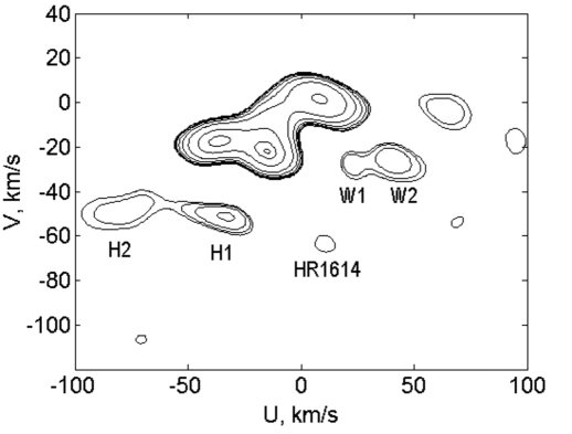
Figure 1: Wavelet map of $UV$ velocities constructed using $\sim$17000 single stars from Hipparcos (1997) with relative parallax errors of no more than 10%.

THE $UV$ VELOCITIES OF THE STREAMS

The wavelet map of the $UV$ velocity distribution for single stars with reliable distance estimates from Bobylev et al. (2010) is presented in Fig. 1. The map was constructed using $\sim$17000 stars from the Hipparcos catalogue (1997). We took their proper motions and parallaxes from a revised version of this catalogue (van Leeuwen 2007) and their radial velocities from the OSACA catalogue of radial velocities (Bobylev et al. 2006) and the Pulkovo compilation of radial velocities (PCRV) (Gontcharov 2006). For all these stars, the relative error in the parallax does not exceed 10%.

The contour lines in Fig. 1 are given on a logarithmic scale: 1, 2, 4, 8, …, 90%, and 99%. The velocities are given relative to the Sun. This figure indicates the W1 and W2 features for the Wolf 630 stream and the H1 and H2 features for the Hercules stream with the following coordinates of their centers: W1 $(U,V)=(21,-26)$ km s^-1, W2 $(U,V)=(40,-24)$ km s^-1, H1 $(U,V)=(-33,-51)$ km s^-1, H2 $(U,V)=(-71,-48)$ km s^-1. According to this map, we selected the specific stars belonging to these features based on the probabilistic method. The number of probable candidates in each stream was the following: 250, 271, 401, and 218 stars in W1, W2, H1, and H2, respectively.

When constructing the Galactic orbits to determine the stellar velocities relative to the local standard of rest (LSR), we use the peculiar solar velocity components relative to the LSR with their values from Schönrich et al. (2010), $(U_{\odot},V_{\odot},W_{\odot})=(11.1,12.2,7.3)\pm(0.7,0.5,0.4)$ km s^-1. When these velocities were determined, the stellar metallicity gradient in the Galactic disk and the effect of radial mixing of stars in the disk were taken into account and modeled. Therefore, the values of these components are currently the most plausible ones and are widely used by various authors.

METHODS

Orbit Construction

We construct the orbits by solving the following system of equations of motion based on a realistic Galactic gravitational potential (Fernández et al. 2008):

$$\begin{array}[]{lll}\ddot{\xi}=-\frac{\displaystyle\partial\Phi}{\displaystyle\partial\xi}-\Omega^{2}_{\odot}(R_{\odot}-\xi)-2\Omega_{\odot}\dot{\eta},\\ \ddot{\eta}=-\frac{\displaystyle\partial\Phi}{\displaystyle\partial\eta}+\Omega^{2}_{\odot}\eta+2\Omega_{\odot}\dot{\xi},\\ \ddot{\zeta}=-\frac{\displaystyle\partial\Phi}{\displaystyle\partial\zeta},\end{array}$$ (1)

where $\Phi$ is the Galactic gravitational potential; the coordinate system $(\xi,\eta,\zeta)$ centered on the Sun rotates around the Galactic center with a constant angular velocity $\Omega_{\odot}$, with the $\xi$ axis being directed to the Galactic center, the $\eta$ axis pointing in the direction of Galactic rotation, and the $\zeta$ axis being directed toward the north Galactic pole; $R_{\odot}$ is the Galactocentric distance of the Sun. When the Galactic potential $\Phi$ is known, the system of equations (1) can be solved numerically. We used a fourth-order Runge–Kutta integrator.

In the model of Allen and Santillán (1991), the Galactocentric distance of the Sun is taken to be $R_{\odot}=8.5$ kpc, while the circular velocity of the Sun around the Galactic center is $V_{\odot}=\Omega_{\odot}R_{\odot}=220$ km s^-1. The Galactic potential considered here consists of an axisymmetric component and a bar potential:

$$\Phi=\Phi_{o}+\Phi_{b}.$$ (2)

In turn, the axisymmetric component can be represented as the sum of three components — central (bulge), disk, and halo ones:

$$\Phi_{o}=\Phi_{C}+\Phi_{D}+\Phi_{H}.$$ (3)

The central component of the Galactic potential in cylindrical coordinates ($r,z,\theta$) is represented as

$$\Phi_{C}=-\frac{M_{C}}{(r^{2}+z^{2}+b^{2}_{C})^{1/2}},$$ (4)

where $M_{C}$ is the mass, $b_{C}$ is the scale length, and $r^{2}=x^{2}+y^{2}.$ The disk component is

$$\Phi_{D}=-\frac{M_{D}}{\{r^{2}+[a_{D}+(z^{2}+b_{D}^{2})^{1/2}]^{2}\}^{1/2}},$$ (5)

where $M_{D}$ is the mass, $a_{D}$ and $b_{D}$ are the scale lengths. The halo component is

$$\Phi_{H}=-\frac{M(R)}{R}-\int_{R}^{100}{{\frac{1}{R^{{}^{\prime}}}}{\frac{dM(R^{{}^{\prime}})}{dR^{{}^{\prime}}}}}dR^{{}^{\prime}},$$ (6)

where

$$M(R)=\frac{M_{H}(R/a_{H})^{2.02}}{1+(R/a_{H})^{1.02}},$$

Here, $M_{H}$ is the mass, $a_{H}$ is the scale length, and $R^{2}=x^{2}+y^{2}+z^{2}.$ The triaxial ellipsoid model (Palou$\breve{s}$ et al. 1993) was chosen as the potential due to the central bar:

$$\Phi_{b}=\frac{M_{b}}{(q_{b}^{2}+x^{2}+[ya_{b}/b_{b}]^{2}+[za_{b}/c_{b}]^{2})^{1/2}},$$ (7)

where $x=R\cos\vartheta,y=R\sin\vartheta$, $a_{b},b_{b},c_{b}$ are the three bar semiaxes, $q_{b}$ is the bar length; $\vartheta=\theta-\Omega_{bar}t-\theta_{bar}$, $\tan\theta=\eta/(R_{\odot}-\xi)$ ($\Omega_{bar}$ is the bar pattern speed, $t$ is the integration time, $\theta_{bar}$ is the bar angle relative to the Galactic $X$ and $Y$ axes).

If $R$ is measured in kpc, $M_{C},M_{D},M_{H},M_{b}$ are in units of the Galactic mass $(M_{G})$ equal to $2.32\times 107M_{\odot},$ then the gravitational constant $G=1$ and 100 km² s^-2 is the unit of measurement of the potential $\Phi$ and its individual components (4)–(7). The parameters of the model potential from Allen and Santillán (1991) and the bar potential adopted here are given in Table 1.

We pass from the moving coordinate system $(\xi,\eta,\zeta)$ to the Galactic one $(X,Y,Z)$ using the formulas

$$\begin{array}[]{lll}X=(R_{\odot}-\xi)\cos(t\Omega_{\odot})-\eta\sin(t\Omega_{\odot}),\\ Y=(R_{\odot}-\xi)\sin(t\Omega_{\odot})+\eta\cos(t\Omega_{\odot}),\\ Z=\zeta.\end{array}$$ (8)

In the case of integration by the Runge–Kutta method, it should be kept in mind that $t=0.001/1.023$ corresponds to one million years at the distance and mass measurements adopted above. The orbit integration time was chosen to be 4 Gyr, given that the characteristic lifetime of the bar (from the beginning of its formation to its destruction) is typically 2–4 Gyr. Note that allowance for the interaction with other galaxies would be required on long integration time scales.

Table 1: Parameters of the Galactic potential model

$M_{C}$	606.0 MG
$M_{D}$	3690.0 MG
$M_{H}$	4615.0 MG
$M_{b}$	43.1 MG
$b_{C}$	0.3873 kpc
$a_{D}$	5.3178 kpc
$b_{D}$	0.2500 kpc
$a_{H}$	12.0 kpc
$q_{b}$	5.0 kpc
$a_{b}/b_{b}$	$1/0.42$
$a_{b}/c_{b}$	$1/0.33$

Searching for Periodic Orbits

This section is devoted to searching for resonant periodic orbits in an axisymmetric potential in a rotating frame lying in the Galactic plane centered at the Galactic center.

Note that the objects execute a three-dimensional motion in accordance with Eqs. (3)–(6) for the potential. However, since the bar rotates around the Galactic center in the $(X,Y)$ plane and since resonant orbits are searched for precisely in the bar rotation frame, we search for periodic orbits in the $(Xp,Yp)$ plane (Fux 2001). We pass from the moving coordinate system $(\xi,\eta)$ to the coordinate system $(X_{p},Y_{p})$ rotating with the pattern speed $\Omega_{p}$ using formulas similar to Eqs. (8):

$$\begin{array}[]{lll}X_{p}=(R_{\odot}-\xi)\cos(t(\Omega_{\odot}-\Omega_{p}))-\eta\sin(t(\Omega_{\odot}-\Omega_{p})),\\ Y_{p}=(R_{\odot}-\xi)\sin(t(\Omega_{\odot}-\Omega_{p}))+\eta\cos(t(\Omega_{\odot}-\Omega_{p})).\end{array}$$ (9)

In this paper, as the rotating frame we consider the bar whose pattern speed and orientation we attempt to estimate by constructing the resonant periodic orbits of stars from the Hercules and Wolf 630 streams in the bar frame. This requires finding the periodic orbits that satisfy the $(2:1)$ resonance (Fux 2001; Orlov and Sotnikova 2007). The condition for a resonance in the stellar disk plane is the commensurability of two frequencies: the angular velocity $\Omega$ and the epicyclic frequency $\kappa$:

$$l\kappa=m(\Omega-\Omega_{p}),$$ (10)

with integers $m\geq 0$ and $l$. In the rotating frame, the $m/l$ resonant orbit is closed after $m$ radial oscillations and $|l|$ orbital periods. Note that condition (10) coincides with the condition for Lindblad resonances only at $l=\pm 1.$ The outside corotation, $l<0,$ is negative, and we can talk about the outer $m/|l|$ resonances. In this paper, we discuss only the outer resonances. Figure 4 from Fux (2001) presents such orbits at $|l|=1.$ If $m=2$ and $l=-1,$ corresponding to $(2:1)$ resonant orbits, then it follows from Eq. (10) that

$$\Omega_{p}=\Omega+\kappa/2.$$ (11)

The ideology of the proposed method is that we seek for the bar pattern speed $\Omega_{p}$ (it is different for different stars) at which the orbit becomes resonant and, hence, periodic (in the case of an axisymmetric potential) and quasi-periodic (in the case of a nonaxisymmetric potential, for example, when the bar is included, see below). We propose the following numerical algorithm of seeking for such a pattern speed $\Omega_{p}$ lying within the range $[\Omega_{1},\Omega_{2}]$ predetermined empirically:

(1) For a given frequency range, we specify a grid of discrete frequencies $\Omega_{1}+m\Delta\Omega,m=0,...,M$, where $\Delta\Omega=(\Omega_{2}-\Omega_{1})/M$, $M$ is an integer large enough to obtain the required dense grid of frequencies. Experience shows that an acceptable accuracy of the algorithm is achieved at $\Delta\Omega=0.01$ km s^-1 kpc^-1.

(2) We integrate the stellar orbit in the coordinate system $(\xi,\eta)$ for a sufficiently long time (several billion years or tens of revolutions around the Galactic center).

(3) We pass to the coordinate system $(X_{p},Y_{p})$ by successively substituting all of the frequencies from the grid specified above into Eq. (9) as $\Omega_{p}$.

(4) We superimpose a discrete grid on the $(X_{p},Y_{p})$ plane with the same step $\Delta x=\Delta y=\Delta$ in the $X$ and $Y$ directions that is chosen empirically to be small enough to provide the required orbit reproduction accuracy. The product $\Delta\times N$, where $N$ is the maximum number of cells in both $X$ and $Y$ directions, gives the linear size of the $(X_{p},Y_{p})$ map. In our case, this size at $N=512$ and the discretization step $\Delta=46.875$ pc is 24 kpc.

(5) On the discrete $N\times N$ $(X_{p},Y_{p})$ plane, we assign “1” to the coordinates of the cell through which the orbit passes and “0” to all the remaining discrete coordinates. If the orbit crosses a given cell several times, then we anyway assign “1” to the corresponding point on the plane only once.

(6) For all maps, we count the number of ones $K.$ The map with the smallest number of ones corresponds to the orbit with a resonance frequency $\Omega_{1}+i\Delta\Omega$, where $i$ is the map number.

(7) For the orbit found, we additionally check whether it belongs to a certain type of resonant orbits (corotation, $1:1,2:1,$ etc.).

Stable periodic orbits give a filling in the form of a trajectory whose shape does not change with increasing number of revolutions around the Galactic center. If several stable periodic orbits fall within a given frequency range, then the algorithm chooses the orbit with the smallest filling to which the orbit with the smallest multiplicity of resonance frequencies corresponds. If the orbit is not stable, then it progressively densely fills a certain space on the $(X_{p},Y_{p})$ coordinate plane with increasing integration time or number of revolutions around the Galactic center, i.e., the number $K$ increases noticeably. Thus, the change in $K$ with integration time serves as a measure of orbit stability. Obviously, the number $K$ depends on the map cell size, so that the numbers for a given object at different frequencies from the frequency range $[\Omega_{1},\Omega_{2}]$ must be compared for discrete maps with the same discretization step.

Once the periodic orbits in the axisymmetric potential (3) had been found, we checked how much the resonance frequencies changed when the bar was included. For this purpose, in the vicinity of the resonance frequency found, we refined its value using the algorithm described above by taking into account the fact that the bar pattern speed and angle are the parameters that enter into the expression for the bar potential in accordance with Eq. (7). As the bar angle we used the estimate obtained for the axisymmetric potential. It turned out that including the bar changed the resonance frequency, on average, by 0.4%. For example, for one of the stars from the Hercules stream with coordinates $(x,y,z,U,V,W)=(0.041,-0.031,-0.128,-42.75,-56,70,-6.26)$ (the positions in kpc, the velocities in km s^-1), the resonance frequency was found to be 52.74 and 52.91 km s^-1 kpc^-1 in the case of the axisymmetric potential and with the inclusion of the bar potential, respectively. The orbits found for this star are shown in Fig. 2. As can be seen from this figure, the orbits in the rotating bar frame obtained in these two cases differ visually, but not much. This is because the gravitational contribution of the bar to the total Galactic potential is small (Fernández et al. 2008). At the same time, however, the orbit acquires the property of stochasticity. As can be seen from Fig. 2, the orbit under the influence of the bar (right panel) becomes more blurred (because it undergoes libration near the resonance) than the periodic resonant orbit obtained in the axisymmetric potential (left panel). Thus, the orbit becomes quasi-periodic under the influence of the bar. As our integration showed, the filling of the plane in the second case slowly but expands with increasing integration time. For example, the number of ones $K$ in the $(X_{p},Y_{p})$ coordinate plane, in our case of size $512\times 512$, evolves as follows: $K=838,1398,1916,$ and 2378 at the integration time $T=1100,2200,3300,$ and 4400 Myr, respectively.

As a result, it turned out that when the bar was included, the resonance frequencies changed by a negligibly small value, while the shape and orientation of orbits in the bar frame did not change. Thus, we showed that to solve our problem of determining the bar pattern speed and orientation, it would suffice to study the periodic orbits obtained in the axisymmetric potential. This is important, because the bar potential is not known with certainty; there are a multitude of its models in the literature. We only know that its gravitational contribution to the total Galactic potential is small.

The influence of the bar was studied in detail using simulations by Fux (2001). We do not set such a goal in this paper. We need to solve the inverse problem: to estimate the parameters of the bar by assuming that the features of the Hercules and Wolf 630 streams are produced by its long-term dynamical effect.

The bar orientation in the Galactic $(X,Y)$ plane can be determined from the orientation of orbits in the $(X_{p},Y_{p})$ plane. Indeed, while in the axisymmetric case the orientation of the resonant orbits is arbitrary, the virtual introduction of a bar will retain only those orbits which are reflection-symmetric with respect to at least one of the bar principal axes (Fux 2001).

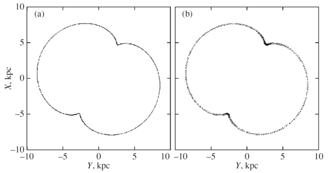
Figure 2: Example of orbit integration in a coordinate system rotating with the bar pattern speed in the axisymmetric potential (a) and with the addition of the bar potential (b); the Galactic center lies at the coordinate origin; the Sun’s coordinates are $(X,Y)=(8.5,0)$ kpc.

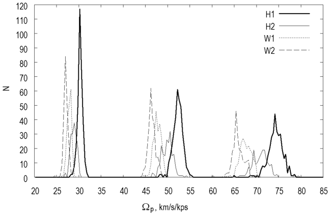
Figure 3: Distributions of the number of stars $N$ (the number of periodic orbits) as a function of the resonance frequency $\Omega_{p}$.

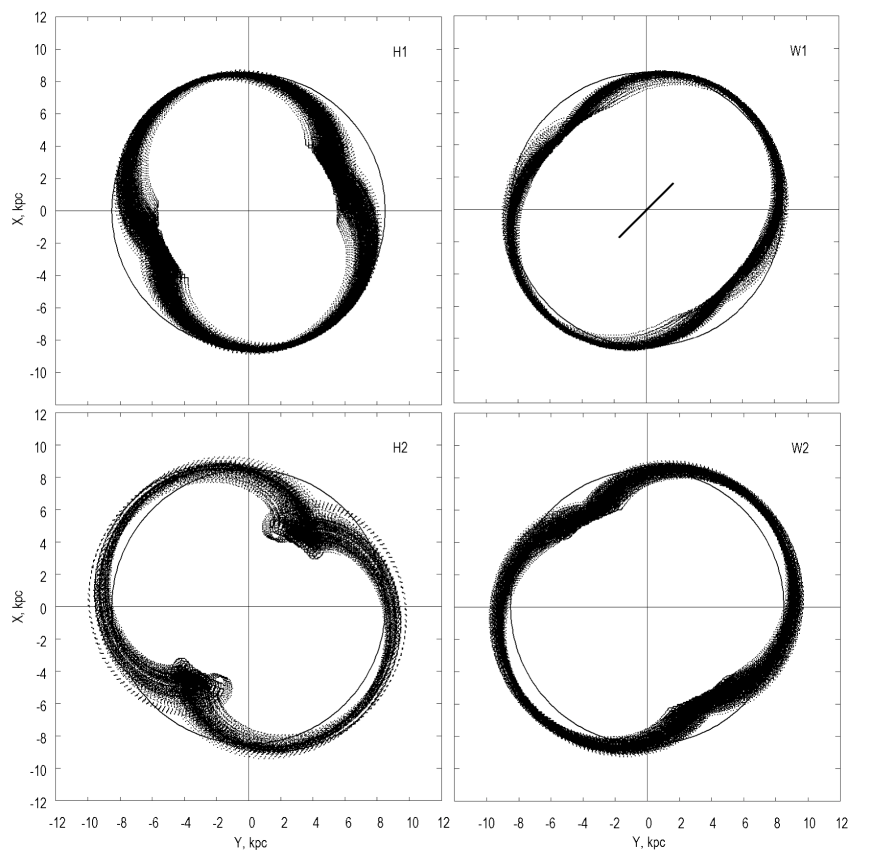
Figure 4: Examples of resonant periodic orbits in a coordinate system rotating with the bar pattern speed. Each graph presents a circumference of radius $R_{0}=8.5$ kpc; the Galactic center lies at the coordinate origin; the Sun’s coordinates are $(X,Y)=(8.5,0)$ kpc; the upper right graph schematically shows the bar oriented at an angle of about $45^{\circ}$ to the Sun’s direction.

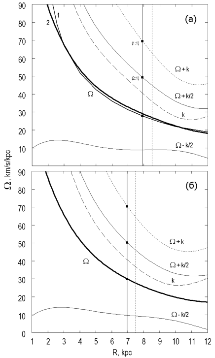
Figure 5: Galactic rotation curve constructed with $R_{0}=8.5$ (a) and $7.5$ (b) kpc; the Sun’s position on both graphs is marked by the vertical dotted line, $R$ is the Galactocentric distance of the star.

RESULTS

Using the above-described method of searching for periodic orbits in an axisymmetric potential for each star of the identified H1, H2, W1, and W2 features, we found the resonance frequencies $\Omega_{c}$, $\Omega_{1:1}$ and $\Omega_{2:1}$. The interval of integration was 4 Gyr.

The corresponding histograms, i.e., the distributions of the number of stars $N$ as a function of the resonance frequency, are presented in Fig. 3. The histograms occupying the left, right, and central parts of the graph refer to the corotation, 1:1, and 2:1 resonance frequencies, respectively. We associate the bar pattern speed below denoted by $\Omega_{bar}$ with the 2:1 resonance frequency. The individual distributions are seen to be Gaussian. The 1:1 resonant and corotation resonant orbits exhibit the largest and smallest dispersions, respectively. The 2:1 resonant orbits, in accordance with Eq. (10), are intermediate between them.

Figure 4 presents the families of orbits in a coordinate system rotating with the bar pattern speed. The orbits of stars in the H1 and H2 streams are elongated perpendicularly to the bar major axis, while the orbits of stars in the W1 and W2 streams are elongated along the bar. As can be seen from Fig. 4, the bar angle $\theta_{bar}$ lies within the range $40^{\circ}-60^{\circ}$. Thus, the bar angle is determined by the inclination of the orbital major axis, as shown in Fig. 4 (upper right panel). In accordance with the central limit theorem, we assume that the deviations of the orbital inclinations of stars from the samples considered obey a normal law. The bar angle for each sample was calculated as the mean of the orbital inclinations of stars from the samples; the error in the angle was calculated as the root–mean–square deviation from the mean.

The quantitative estimates of $\Omega_{bar}$ and $\theta_{bar}$ found from the results presented in Figs. 3 and 4 are given in Table 2. As can be seen from the table, the bar pattern speed $\Omega_{bar}$ and the bar angle $\theta_{bar}$ determined from the pair of W2 and H1 have larger discrepancies between themselves than those from the pair of W1 and H2.

Let us show that our estimates are robust when using the various Galactic rotation curves constructed with the constant $R_{0}$ whose values lie within a fairly wide range, from 7.5 to 8.5 kpc.

Figure 5a provides the Galactic rotation curves no. 1 from the tabulated data of Allen and Santillán (1991) and no. 2 from the same initial data that were used in Bobylev et al. (2008) but constructed with $R_{0}=8.5$ kpc.

Bobylev et al. (2008) used data on the three dimensional space velocity field of young open star clusters and the radial velocities of HI clouds and HII regions. The rotation curve no. 2 was determined by using the first six terms of the Taylor expansion of the angular velocity of Galactic rotation $\Omega$ in Bottlinger’s equations. The terms of the series found at $R_{0}=8.5$ kpc are $\Omega_{0}=-26.96\pm 0.58$ km s^-1 kpc^-1, $\Omega^{1}_{0}=3.52\pm 0.07$ km s^-1 kpc^-2, $\Omega^{2}_{0}=-0.470\pm 0.046$ km s^-1 kpc^-3, $\Omega^{3}_{0}=0.042\pm 0.032$ km s^-1 kpc^-4, $\Omega^{4}_{0}=-0.218\pm 0.019$ km s^-1 kpc^-5, $\Omega^{5}_{0}=0.108\pm 0.013$ km s^-1 kpc^-6, where $\Omega_{0},\Omega^{1}_{0},...,\Omega^{5}_{0}$ are the angular velocities and the corresponding derivatives at $R=R_{0},$ and $R$ is the Galactocentric distance of the star. The Oort constants are $A=14.94\pm 0.28$ km s^-1 kpc^-1 and $B=-12.02\pm 0.65$ km s^-1 kpc^-1.

It can be seen from Fig. 5a that curves 1 and 2 have significant differences only at $R<2.5$ kpc, which is not critical for our goals. Curve 2 has an analytical representation, which allows the dependences $k(R)=2\Omega(1+1/2\cdot R/\Omega\cdot d\Omega/dR)^{1/2}$, $\Omega+k/2$, $\Omega-k/2,$ and $\Omega+k$ shown in Fig. 5 to be calculated. The vertical dotted line in Fig. 5a marks the distance $R_{0}=8.5$ kpc, the thin vertical line indicates the radius of the outer Lindblad resonance (OLR) $R_{OLR}=7.9$ kpc (we found $R_{OLR}=0.93R_{0}$ based on the data in Fig. 3 from the mean of the four corresponding frequencies), the three resonances of interest to us are marked: the corotation, (2:1), and (1:1) ones. According to present-day estimates, the exact value of R0 lies within the range 7.1–8.5 kpc (see, e.g., Table 1 from Foster and Cooper (2010)). Therefore, it is of interest to trace whether the positions of the resonances change with $R_{0}.$ Figure 5b provides the rotation curve constructed directly from the data of Bobylev et al. (2008) at $R_{0}=7.5$ kpc. As can be seen from Fig. 5, when $R_{0}$ decreases by 1 kpc, the resonance frequencies remain almost unchanged at $R_{OLR}=0.93R_{0}.$ As we see from the graphs, the bar pattern speed corresponding to the 2:1 resonance frequency is about 52 km s^-1 kpc, consistent with the results that we have obtained above by an independent method.

Table 2: Parameters found from the $H_{1,2}$ and $W_{1,2}$ features

Feature	$\Omega_{bar},$ km s-1 kpc-1	$\theta_{bar},$ deg
$H_{1}$	$52.3\pm 1.1$	$62\pm 11$
$H_{2}$	$49.9\pm 1.2$	$51\pm 9~{}$
$W_{1}$	$47.7\pm 0.9$	$45\pm 10$
$W_{2}$	$46.4\pm 0.9$	$38\pm 9~{}$
Mean	$49.1\pm 1.3$	$49\pm 5~{}$

Table 3: Parameters of the Galactic “short” (the upper part of the table) and “long” (the lower part of the table) bars

$\Omega_{bar},$	$R_{bar},$	$\theta_{bar}$	Source
km s-1 kpc-1	kpc
63	$2.4\pm 0.5$	$16^{\circ}\pm 2^{\circ}$	Binney et al. (1991)
$53\pm 3$	—	—	Dehnen (1999)
$59\pm 5$	—	—	Debattista et al. (2002)
$60\pm 5$	$3.4\pm 0.3$	$20^{\circ}-25^{\circ}$	Bissantz et al. (2003)
—	—	$11.1^{\circ}\pm 0.7^{\circ}$	Robin et al. (2003)
—	$2.5-3.0$	$22^{\circ}\pm 5.5^{\circ}$	Babusiaux and Gilmore (2005)
—	—	$20^{\circ}-35^{\circ}$	López-Corredoira et al. (2005)
—	—	$12.6^{\circ}\pm 3.2^{\circ}$	Cabrera-Lavers et al. (2007)
$57.4^{+2.8}_{-3.3}$	—	$0^{\circ}-30^{\circ}$	Chakrabarty (2007)
—	—	$24^{\circ}-27^{\circ}$	Rattenbury et al. (2007)
$57.7$	—	—	Gardner and Flinn (2010)
—	$3$	$20^{\circ}-25^{\circ}$	Bobylev et al. (2014)
$56\pm 2$	—	—	Antoja et al. (2014)
—	—	$44^{\circ}$	Sevenster et al. (1999)
—	$4.4\pm 0.5$	$44^{\circ}\pm 10^{\circ}$	Benjamin et al. (2005)
—	—	$43^{\circ}\pm 17^{\circ}$	Groenewegen and Blommaert (2005)
—	$3.9$	$43^{\circ}\pm 7^{\circ}$	López-Corredoira et al. (2007)
—	$4$	$43.0^{\circ}\pm 1.8^{\circ}$	Cabrera-Lavers et al. (2007)
$56.7$	—	—	Gardner and Flinn (2010)
$49.1\pm 1.3$	$4.2\pm 0.7$	$49^{\circ}\pm 5^{\circ}$	this paper

DISCUSSION

Let us first discuss some of the known bar characteristics. Table 3 gives the estimates of the bar pattern speed, size, and orientation obtained by different authors using different data. The characteristics of both classical “short” and “long” bars are given.

Binney et al. (1991) and Bissantz et al. (2003) estimated the parameters by comparing the radio observations of central Galactic regions (HI, CO) with various bar models.

Debattista et al. (2002) estimated the bar pattern speed from radio observations of 250 OH/IR stars. These are oxygen-rich stars with envelopes at the asymptotic-giant-branch phase with strong mass loss. The observations yielded $\Delta V\equiv\Omega_{bar}R_{0}-V_{LSR}=252\pm 41$ km s^-1, while $\Omega_{bar}$ was calculated at $R_{0}=8$ kpc and $V_{LSR}=220$ km s^-1. Thus, this is a rare example of a direct measurement of the bar pattern speed. The same stars were also used in Sevenster et al. (1999).

Benjamin et al. (2005) estimated the size and orientation of the long bar by analyzing the star counts based on the GLIMPSE (Galactic Legacy Infrared Mid-Plane Survey Extraordinaire) infrared survey produced on the basis of observations with the Spitzer Space Telescope. For these purposes, Groenewegen and Blommaert (2007) used Mira variables from the OGLE-II survey (Wozniak et al. 2002), designed to search for microlensing effects. The arguments for the hypothesis of a long bar were also presented by López-Corredoira et al. (2007). Shortly afterwards, based on the counts of stars from the 2MASS catalog, this group of authors (Cabrera-Lavers et al. 2007) proposed a two-bar model.

A similar method of star counts was applied using red-giant-clump stars from the CIRSI (Cambridge InfraRed Survey Instrument) survey by Babusiaux and Gilmore (2005), from the 2MASS catalog by López-Corredoira et al. (2005), and from the OGLE-II survey by Rattenbury et al. (2007). Robin et al. (2003) extracted information about the bar size and orientation by analyzing the data from the Hipparcos catalogue (1997).

Dehnen (1999), Chakrabarty (2007), and Gardner and Flinn (2010) estimated the bar parameters based on simulations to explain the observed bimodal $UV$ velocity distribution of solar-neighborhood stars. It is important to note that one of the models in Gardner and Flinn (2010) contained two bars for which close pattern speeds were found. This means that the two bars can rotate almost synchronously.

Bobylev et al. (2014) estimated the bar orientation parameters using the XPM catalog (Fedorov et al. 2010), which contains the proper motions of millions of stars. There are photometric data from the 2MASS catalog for these stars, which allowed the photometric distances to be estimated, while using the proper motions allowed one to eliminate the foreground stars and literally to “see” the bar.

Antoja et al. (2014) found the bar pattern speed by comparing their analytical bar model with stars from the RAVE4 catalog. Distance estimates and highly accurate radial velocities are available for these stars. In the model of these authors, the Hercules stream was assumed to be produced by the influence of the bar and the Galactic spiral structure.

Table 3 does not encompass all of the known results. Note that quite a large selection of Galactic bar parameter determinations can be found in Vanhollebeke et al. (2009).

The resonant orbits we found show that the bar pattern speed $\Omega_{bar}$ lies within the range 45–55 km s^-1 kpc^-1, while the bar angle $\Omega_{bar}$ is within the range $40^{\circ}-60^{\circ}.$ The results obtained are consistent with the view that the Hercules and Wolf 630 streams could be formed by a single mechanism associated with the splitting of the $UV$ velocity plane under the influence of the Galactic bar.

Our results are in agreement with the simulations of Dehnen (1999) for $R_{OLR}\approx 0.9R_{0}.$ The bar size estimated from the rotation curve by taking into account the confidence region for $\Omega_{bar}$ is $R_{bar}=4.2\pm 0.7$ kpc (for the adopted $R_{0}=8$ kpc). As can be seen from Table 3, this resembles a long bar.

CONCLUSIONS

We analyzed the four most significant features in the $UV$ velocity distribution of solar-neighborhood stars: H1, H2 from the Hercules stream and W1, W2 from the Wolf 630 stream with the $(U,V)$ coordinates of their centers $(-33,-51),(-71,-48),(21,-26),$ and $(40,-24)$ km s^-1, respectively. Based on the assumption that the Hercules and Wolf 630 streams were induced by the central Galactic bar, we formulated the problem of determining the bar characteristics independently from each of the identified features.

To construct the Galactic orbits of the individual stars forming these streams, we used the model of Allen and Santillán (1991). From the set of constructed orbits, we selected only the stable orbits in resonance with the bar. Analysis of the resonant orbits found showed that the bar pattern speed $\Omega_{bar}$ lies within the range 45–55 km s^-1 kpc^-1 with a mean of $49.1\pm 1.3$ km s^-1 kpc^-1, while the bar angle is within the range $40^{\circ}-60^{\circ}$ with a mean of $49\pm 5^{\circ}.$ These estimates were shown to be robust when using the various Galactic rotation curves constructed with the constant $R_{0}$ whose values lie within a fairly wide range, from 7.5 to 8.5 kpc.

The results obtained are consistent with the view that the Hercules and Wolf 630 streams could be formed by a single mechanism associated with the fact that a long-term influence of the Galactic bar led to a characteristic bimodal splitting of the $UV$ velocity plane.

ACKNOWLEDGMENTS

We are grateful to the referees for their helpful remarks that contributed to an improvement of this paper. This work was supported by the “Transitional and Explosive Processes in Astrophysics” Program P–41 of the Presidium of Russian Academy of Sciences.

REFERENCES

1. C. Allen and A. Santillán, Rev. Mex. Astron. Astrof. 22, 255 (1991).

2. T. Antoja, F. Figueras, D. Fernández, and J. Torra, Astron. Astrophys. 490, 135 (2008).

3. T. Antoja, O. Valenzuela, B. Pichardo, E. Moreno, F. Figueras, and D. Fernández, Astrophys. J. 700, L78 (2009).

4. T. Antoja, A. Helmi, W. Dehnen, O. Bienaymé, J. Bland-Hawthorn, B. Famaey, K. Freeman, B.K. Gibson, et al., Astron. Astrophys. 563, 60 (2014).

5. R. Asiain, F. Figueras, J. Torra, and B. Chen, Astron. Astrophys. 341, 427 (1999).

6. C. Babusiaux and G. Gilmore, Mon. Not. R. Astron. Soc. 358, 1309 (2005).

7. R.A. Benjamin, E. Churchwell, B.L. Babler, R. Indebetouw, M.R. Meade, B.A. Whitney, C. Watson, M.G. Wolfire, et al., Astrophys. J. 630, L149 (2005).

8. T. Bensby, M.S. Oey, S. Feltzing, and B. Gustafsson, Astrophys. J. 655, L89 (2007).

9. J. Binney, O.E. Gerhard, A. Stark, J. Bally, and K.I. Uchida, Mon. Not. R. Astron. Soc. 252, 210 (1991).

10. N. Bissantz, P. Englmaier, and O. Gerhard, Mon. Not. R. Astron. Soc. 340, 949 (2003).

11. V.V. Bobylev, G.A. Gontcharov, and A.T. Bajkova, Astron. Rep. 50, 733 (2006).

12. V.V. Bobylev and A.T. Bajkova, Astron. Rep. 51, 372 (2007).

13. V.V. Bobylev, A.T. Bajkova, and A.S. Stepanishchev, Astron. Lett. 34, 515 (2008).

14. V.V. Bobylev, A.T. Bajkova, and A.A. Mylläri, Astron. Lett. 36, 27 (2010).

15. V.V. Bobylev, A.V. Mosenkov, A.T. Bajkova, and G.A. Gontcharov, Astron. Lett. 40, 86 (2014).

16. J. Bovy, Astrophys. J. 725, 1676 (2010).

17. E.J. Bubar and J.R. King, Astron. J. 140, 293 (2010).

18. A. Cabrera-Lavers, P.L. Hammersley, C. González-Fernández, M. López-Corredoira, F. Garzón, and T.J. Mahoney, Astron. Astrophys. 465, 825 (2007).

19. D. Chakrabarty, Astron. Astrophys. 467, 145 (2007).

20. E. Chereul, M. Crézé, and O. Bienaymé, Astron. Astrophys. 340, 384 (1998).

21. V.P. Debattista, O. Gerhard, and M.N. Sevenster, Mon. Not. R. Astron. Soc. 334, 355 (2002).

22. W. Dehnen, Astron. J. 115, 2384 (1998).

23. W. Dehnen, Astrophys. J. 524, L35 (1999).

24. W. Dehnen, Astron. J. 119, 800 (2000).

25. O.J. Eggen, Publ. Astron. Soc. Pacif. 81, 553 (1969).

26. B. Famaey, A. Jorissen, X. Luri, M. Mayor, S. Udry, H. Dejonghe, and C. Turon, Astron. Astrophys. 430, 165 (2005).

27. P.N. Fedorov, V.S. Akhmetov, V.V. Bobylev, and A.T. Bajkova, Mon. Not. R. Astron. Soc. 406, 1734 (2010).

28. D. Fernández, F. Figueras, and J. Torra, Astron. Astrophys. 480, 735 (2008).

29. T. Foster and B. Cooper, ASP Conf. Ser. 438, 16 (2010).

30. C. Francis and E. Anderson, New Astron. 14, 615 (2009).

31. R. Fux, Astron. Astrophys. 373, 511 (2001).

32. E. Gardner and C. Flinn, Mon. Not. R. Astron. Soc. 405, 545 (2010).

33. G.A. Gontcharov, Astron. Lett. 32, 795 (2006).

34. M.A.T. Groenewegen and J.A.D.L. Blommaert, Astron. Astrophys. 443, 143 (2005).

35. The Hipparcos and Tycho Catalogues, ESA SP-1200 (1997).

36. F. van Leeuwen, Astron. Astrophys. 474, 653 (2007).

37. M. López-Corredoira, A. Cabrera-Lavers, and O.E. Gerhard, Astron. Astrophys. 439, 107 (2005).

38. M. López-Corredoira, A. Cabrera-Lavers, T.J. Mahoney, P.L. Hammersley, F. Garzón, and C. González-Fernández, Astron. J. 133, 154 (2007).

39. V.V. Orlov and N.Ya. Sotnikova, in Astronomy: Traditions, Present, Future, Ed. by V.V. Orlov, I.P. Reshetnikov, and N.Ya. Sotnikova (SPb Gos. Univ., St. Petersburg, 2007), p. 169 [in Russian].

40. J. Palou$\breve{s}$, B. Jungwiert, and J. Kopeck$\acute{y}$, Astron. Astrophys. 274, 189 (1993).

41. L. Pompeia, T. Masseron, B. Famaey, S. van Eck, A. Jorissen, I. Minchev, A. Siebert, C. Sneden, et al., Mon. Not. R. Astron. Soc. 415, 1138 (2011).

42. A.C. Quillen and I. Minchev, Astron. J. 130, 576 (2005).

43. N.J. Rattenbury, S. Mao, T. Sumi, and M.C. Smith, Mon. Not. R. Astron. Soc. 378, 1064 (2007).

44. A.C. Robin, C. Reylé, S. Derriére, and S. Picaud, Astron. Astrophys. 409, 523 (2003).

45. R. Schönrich, J. Binney, and W. Dehnen, Mon. Not. R. Astron. Soc. 403, 1829 (2010).

46. M. Sevenster, P. Saha, D. Valls-Gabaud, and R. Fux, Mon. Not. R. Astron. Soc. 307, 584 (1999).

47. R.S. de Simone, X. Wu, and S. Tremain, Mon. Not. R. Astron. Soc. 350, 627 (2004).

48. J. Skuljan, J.B. Hearnshaw, and P.L. Cottrell, Mon. Not. R. Astron. Soc. 308, 731 (1999).

49. E. Vanhollebeke, M.A.T. Groenewegen, and L. Girardi, Astron. Astrophys. 498, 95 (2009).

50. P.R. Wozniak, A. Udalski, M. Szymanski, M. Kubiak, G. Pietrzynski, I. Soszynski, and K. Zebrun, Acta Astron. 52, 129 (2002).