Distributed Spectral Efficiency Maximization in Full-Duplex Cellular Networks

Abstract

Three-node full-duplex is a promising new transmission mode between a full-duplex capable wireless node and two other wireless nodes that use half-duplex transmission and reception respectively. Although three-node full-duplex transmissions can increase the spectral efficiency without requiring full-duplex capability of user devices, inter-node interference – in addition to the inherent self-interference – can severely degrade the performance. Therefore, as methods that provide effective self-interference mitigation evolve, the management of inter-node interference is becoming increasingly important. This paper considers a cellular system in which a full-duplex capable base station serves a set of half-duplex capable users. As the spectral efficiencies achieved by the uplink and downlink transmissions are inherently intertwined, the objective is to device channel assignment and power control algorithms that maximize the weighted sum of the uplink-downlink transmissions. To this end a distributed auction based channel assignment algorithm is proposed, in which the scheduled uplink users and the base station jointly determine the set of downlink users for full-duplex transmission. Realistic system simulations indicate that the spectral efficiency can be up to $89\,\mathrm{\%}$ better than using the traditional half-duplex mode. Furthermore, when the self-interference cancelling level is high, the impact of the user-to-user interference is severe unless properly managed.

I Introduction

Traditional cellular networks operate in half-duplex (HD) transmission mode, in which a user equipment (UE) or the base station (BS) either transmits or receives on any given frequency channel. However, the increasing demand to support the transmission of unprecedented data quantities has led the research community to investigate new wireless transmission technologies. Recently, in-band full duplex (FD) has been proposed as a key enabling technology to drastically increase the spectral efficiency of conventional wireless transmission modes. Due to recent advances in antenna design, interference cancellation algorithms, self-interference (SI) suppression techniques and prototyping of FD transceivers, FD transmission is becoming a realistic technology component of advanced wireless – including cellular – systems, especially in the low transmit power regime [1, 2].

In particular, in-band FD and three node full duplex (TNFD) transmission modes can drastically increase the spectral efficiency of conventional wireless transmission modes since both transmission techniques have the potential to double the spectral efficiency of traditional wireless systems operating in HD [3, 4]. TNFD involves three nodes, but only one of them needs to have FD capability. The FD-capable node transmits to its receiver node while receiving from another transmitter node on the same frequency channel.

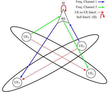
Figure 1: A cellular network employing FD with two UEs pairs. The base station selects pairs of UEs, represented by the ellipses, and jointly schedules them for FD transmission by allocating frequency channels in the UL and DL. To mitigate UE-to-UE interference, it is advantageous to co-schedule DL/UL users for FD transmission that are far apart, such as $\text{UE}_{1}$-$\text{UE}_{2}$ and $\text{UE}_{3}$-$\text{UE}_{4}$.

As illustrated in Figure 1, FD operation in a cellular environment experiences new types of interference, aside from the inherently present SI. Because the level of UE-to-UE interference depends on the UE locations and their transmission powers, coordination mechanisms are needed to mitigate the negative effect of the interference on the spectral efficiency of the system [5]. A key element of such mechanisms is UE pairing and frequency channel selection that together determine which UEs should be scheduled for simultaneous UL and DL transmissions on specific frequency channels. Hence, it is crucial to design efficient and fair medium access control protocols and physical layer procedures capable of supporting adequate pairing mechanisms. Furthermore, in future cellular networks the idea is to move from a fully centralized to a more distributed network [6], where the infrastructure of the BS can be used to help the UEs to communicate in a distributed manner and reduce the processing burden at the BS, which is further increased by SI cancellation.

To the best of our knowledge, the only work to consider a distributed approach for FD cellular networks is reported in [7]. However, the authors tackle the problem of the UE-to-UE interference from an information theoretic perspective, without relating to resource allocation and power control. Conversely, some works consider the joint subcarrier and power allocation problem [8] and the joint duplex mode selection, channel allocation, and power control problem [9] in FD networks. The cellular network model in [8] is applicable to FD mobile nodes rather than to networks operating in TNFD mode. The work reported in [9] considers the case of TNFD transmission mode in a cognitive femto-cell context with bidirectional transmissions from UEs and develops sum-rate optimal resource allocation and power control algorithms. However, none of these two works consider a distributed approach for FD cellular networks.

In this paper we formulate the joint problem of user pairing (i.e. co-scheduling of UL and DL simultaneous transmissions on a frequency channel), and UL/DL power control as a mixed integer nonlinear programming (MINLP) problem, whose objective is to maximize the overall spectral efficiency of the system. Due to the complexity of the MINLP problem proposed, our solution approach relies on Lagrangian duality and a distributed auction algorithm in which UL users offer bids on desirable DL users. In this iterative auction process, the BS – as the entity that owns the radio resources – accepts or rejects bids and performs resource assignment. This algorithm is tested in a realistic system simulator that indicates that the bidding process converges to a near optimal pairing and power allocation.

II System Model and Problem Formulation

II-A System Model

We consider a single-cell cellular system in which only the BS is FD capable, while the UEs served by the BS are only HD capable, as illustrated by Figure 1. In Figure 1, the BS is subject to SI and the UEs in the UL ($\text{UE}_{2}$ and $\text{UE}_{4}$) cause UE-to-UE interference to co-scheduled UEs in the DL, that is to $\text{UE}_{1}$ and $\text{UE}_{3}$ respectively. The number of UEs in the UL and DL is denoted by $I$ and $J$, respectively, which are constrained by the total number of frequency channels in the system $F$, i.e., $I\leq F$ and $J\leq F$. The sets of UL and DL users are denoted by by $\mathcal{I}=\{1,\ldots,I\}$ and $\mathcal{J}=\{1,\ldots,J\}$ respectively.

We consider frequency flat and slow fading, such that the channels are constant during the time slot of a scheduling instance and over the frequency channels assigned to co-scheduled users. Let $G_{ib}$ denote the effective path gain between transmitter UE $i$ and the BS, $G_{bj}$ denote the effective path gain between the BS and the receiving UE $j$, and $G_{ij}$ denote the interfering path gain between the UL transmitter UE $i$ and the DL receiver UE $j$. To take into account the residual SI power that leaks to the receiver, we define $\beta$ as the SI cancellation coefficient, such that the SI power at the receiver of the BS is $\beta P_{j}^{d}$ when the transmit power is $P_{j}^{d}$.

The vector of transmit power levels in the UL by UE $i$ is denoted by $\mathbf{p^{u}}=[P_{1}^{u}\ldots P_{I}^{u}]$, whereas the DL transmit powers by the BS is denoted by $\mathbf{p^{d}}=[P_{1}^{d}\ldots P_{J}^{d}]$. As illustrated in Figure 1, the UE-to-UE interference is much dependent on the geometry of the co-scheduled UL and DL users, i.e., the pairing of UL and DL users. Therefore, UE pairing is a key functions of the system. Accordingly, we define the assignment matrix, $\mathbf{X}\in\{0,1\}^{I\times J}$, such that

$$x_{ij}=\begin{cases}1,&\text{if the UL $\text{UE}_{i}$ is paired with the DL $\text{UE}_{j}$},\\ 0,&\text{otherwise.}\end{cases}$$

The signal-to-interference-plus-noise ratio (SINR) at the BS of transmitting user $i$ and the SINR at the receiving user $j$ of the BS are given by

$$\gamma_{i}^{u}=\frac{P_{i}^{u}G_{ib}}{\sigma^{2}+\sum_{j=1}^{J}x_{ij}P_{j}^{d}\beta},\;\gamma_{j}^{d}=\frac{P_{j}^{d}G_{bj}}{\sigma^{2}+\sum_{i=1}^{I}x_{ij}P_{i}^{u}G_{ij}},$$ (1)

respectively, where $x_{ij}$ in the denominator of $\gamma_{i}^{u}$ accounts for the SI at the BS, whereas $x_{ij}$ in the denominator of $\gamma_{j}^{d}$ accounts for the UE-to-UE interference caused by $\text{UE}_{i}$ to $\text{UE}_{j}$.

Thus, the achievable spectral efficiency for each user is given by the Shannon equation (in bits/s/Hz) for the UL and DL as $C_{i}^{u}=\log_{2}(1+\gamma_{i}^{u})$ and $C_{j}^{d}=\log_{2}(1+\gamma_{j}^{d})$, respectively. In addition to the spectral efficiency, we consider weights for the UL and DL users, which are denoted by $\alpha_{i}^{u}$ and $\alpha_{j}^{d}$, respectively. The idea behind weighing is that it allows the system designer to choose between the commonly used sum rate maximization and important fairness related criteria such as the well known path loss compensation typically employed in the power control of cellular networks [10]. For the weights $\alpha_{i}^{u}$ and $\alpha_{j}^{d}$, we can account for sum rate maximization with $\alpha_{i}^{u}=\alpha_{j}^{d}=1$ and for path loss compensation with $\alpha_{i}^{u}=G_{ib}^{-1}$ and $\alpha_{j}^{d}=G_{bj}^{-1}$.

II-B Problem Formulation

Our goal is to jointly consider the assignment of UEs in the UL and DL (pairing), while maximizing the weighted sum spectral efficiency of all users. Specifically, the problem is formulated as

$$\underset{\mathbf{X},\mathbf{p}^{u},\mathbf{p}^{d}}{\text{maximize}}\quad \sum_{i=1}^{I}\alpha_{i}^{u}C_{i}^{u}+\sum_{j=1}^{J}\alpha_{j}^{d}C_{j}^{d}$$ (2a)

subject to $$\gamma_{i}^{u}\geq\gamma_{\text{th}}^{u},\;\forall i,$$ (2b)

$$\gamma_{j}^{d}\geq\gamma_{\text{th}}^{d},\;\forall j,$$ (2c)

$$P_{i}^{u}\leq P_{\text{max}}^{u},\;\forall i,$$ (2d)

$$P_{j}^{d}\leq P_{\text{max}}^{d},\;\forall j,$$ (2e)

$$\sum_{i=1}^{I}x_{ij}\leq 1,\;\forall j,$$ (2f)

$$\sum_{j=1}^{J}x_{ij}\leq 1,\;\forall i,$$ (2g)

$$x_{ij}\in\{0,1\},\;\forall i,j.$$ (2h)

The main optimization variables are $\mathbf{p}^{u}$, $\mathbf{p}^{d}$ and $\mathbf{X}$. Constraints (2b) and (2c) ensure a minimum SINR to be achieved in the DL and UL, respectively. Constraints (2d) and (2e) limit the transmit powers whereas constraints (2f)-(2g) assure that only one UE in the DL can share the frequency resource with a UE in the UL and vice-versa. Note that constraints (2b)-(2c) require that the SINR targets for both UL and DL be defined a priori.

Problem (2) belongs to the category of MINLP, which is known for its high complexity and computational intractability. Thus, to solve problem (2) we will rely on Lagrangian duality, which is described on Section III. We develop the optimal power allocation for a UL-DL pair and the optimal closed-form solution for the assignment, which can be solved in a centralized manner. However, in future cellular networks the idea is to move from a fully centralized to a more distributed network [6], offloading the burden on the BS. With this objective, in Section IV we use the optimal power allocation to create a distributed solution for the assignment between UL and DL users.

III A Solution Approach Based on Lagrangian Duality

From problem (2), we form the partial Lagrangian function by considering constraints (2b)-(2c) and ignoring the integer (2f)-(2h) and power allocation constraints (2d)-(2e). To this end, we introduce Lagrange multipliers $\boldsymbol{\lambda}^{u},\;\boldsymbol{\lambda}^{d}$, where the superscript $u$ and $d$ denote the dimensions of $I$ and $J$, respectively. The partial Lagrangian is a function of the Lagrange multipliers and the optimization variables $\mathbf{X},\mathbf{p}^{u},\mathbf{p}^{d}$ as follows:

$$L(\boldsymbol{\lambda}^{u},\boldsymbol{\lambda}^{d},\mathbf{X},\mathbf{p}^{u},\mathbf{p}^{d}) \triangleq-\sum_{i=1}^{I}\alpha_{i}^{u}C_{i}^{u}-\sum_{j=1}^{J}\alpha_{j}^{d}C_{j}^{d}+$$

$$+\sum_{i=1}^{I}\lambda_{i}^{u}\Big{(}\gamma_{\text{th}}^{u}-\gamma_{i}^{u}\Big{)}+\sum_{j=1}^{J}\lambda_{j}^{d}\Big{(}\gamma_{\text{th}}^{d}-\gamma_{j}^{d}\Big{)}.$$ (3)

Let $g(\boldsymbol{\lambda}^{u},\boldsymbol{\lambda}^{d})$ denote the dual function obtained by minimizing the partial Lagrangian (III) with respect to the variables $\mathbf{X},\mathbf{p}^{u},\mathbf{p}^{d}$. That is, the dual function is

$$g(\boldsymbol{\lambda}^{u},\boldsymbol{\lambda}^{d}) =\underset{\scriptscriptstyle\mathbf{X}\in\mathcal{X}\;\mathbf{p}^{u},\mathbf{p}^{d}\in\mathcal{P}}{\inf}L(\boldsymbol{\lambda}^{u},\boldsymbol{\lambda}^{d},\mathbf{X},\mathbf{p}^{u},\mathbf{p}^{d}),$$ (4)

where $\mathcal{X}$ and $\mathcal{P}$ are the set where the assignment and power allocation constraints are fulfilled, respectively. Notice that we can rewrite the dual as

$$\textstyle g(\boldsymbol{\lambda}^{u},\boldsymbol{\lambda}^{d})\!=\underset{\scriptscriptstyle\mathbf{X}\in\mathcal{X}\;\mathbf{p}^{u},\mathbf{p}^{d}\in\mathcal{P}}{\inf}\sum\limits_{n=1}^{N}\!\Bigg{(}q_{i_{n}}^{u}(\mathbf{X},\mathbf{p}^{u},\mathbf{p}^{d})+q_{j_{n}}^{d}(\mathbf{X},\mathbf{p}^{u},\mathbf{p}^{d})\Bigg{)},$$ (5)

where we assume $N=I=J$ is the maximum number of UL-DL pairs, $i_{n}$ and $j_{n}$ are the UL and DL users of pair $n$, respectively. Moreover,

$$q_{i_{n}}^{u}(\mathbf{X},\mathbf{p}^{u},\mathbf{p}^{d}) \triangleq\lambda_{i_{n}}^{u}\Big{(}\gamma_{\text{th}}^{u}-\gamma_{i_{n}}^{u}\Big{)}-\alpha_{i}^{u}C_{i_{n}}^{u},$$ (6a)

$$q_{j_{n}}^{d}(\mathbf{X},\mathbf{p}^{u},\mathbf{p}^{d}) \triangleq\lambda_{j_{n}}^{d}\Big{(}\gamma_{\text{th}}^{d}-\gamma_{j_{n}}^{d}\Big{)}-\alpha_{j_{n}}^{d}C_{j_{n}}^{d}.$$ (6b)

We can find the infimum of (5) if we maximize the SINR of the $N$ UL-DL pairs. Thus, we can write a closed-form expression for the assignment $x_{ij}$ as follows:

$$x_{ij}^{\star}=\begin{cases}1,&\text{if }(i,j)=\underset{i,j}{\operatorname*{arg\,max}}\;\Big{(}q_{i_{n}}^{u,\text{max}}+q_{j_{n}}^{d,\text{max}}\Big{)}\\ 0,&\text{otherwise,}\end{cases}$$ (7)

where for simplicity we denoted an ordinary pair as $(i,j)$. Notice that $x_{ij}^{\star}$ and equation (7) uniquely associate an UL user with a DL user. However, the solutions are still tied through the SINRs $\gamma_{i}^{u}$ and $\gamma_{j}^{d}$, i.e., the solution to the assignment problem is still complex and – through (7) – is intertwined with the optimal power allocation.

Since the SINRs on the UL are not separable from those on the DL, we cannot analyse them independently. Consequently, we need to find the powers that jointly minimize (5). To this end, we first analyse the dual problem, given by

$$\underset{\boldsymbol{\lambda}^{u},\;\boldsymbol{\lambda}^{u}}{\text{maximize}} g(\boldsymbol{\lambda}^{u},\boldsymbol{\lambda}^{d})$$ (8a)

subject to $$\lambda_{i}^{u},\;\lambda_{j}^{d},\geq 0,\forall i,j,$$ (8b)

where recall that $g(\boldsymbol{\lambda}^{u},\boldsymbol{\lambda}^{d})$ is the solution of problem (4). Notice that if constraints (2b)-(2c) are fulfilled in the inequality or equality, $\lambda_{i}^{u}\Big{(}\gamma_{\text{th}}^{u}-\gamma_{i}^{u}\Big{)}$ and $\lambda_{j}^{d}\Big{(}\gamma_{\text{th}}^{d}-\gamma_{j}^{d}\Big{)}$ will be either negative or zero. If the terms are negative, then $\lambda_{i}^{u}$ or $\lambda_{j}^{d}$ will be zero. Thus, the terms with $\lambda_{i}^{u}$ and $\lambda_{j}^{d}$ will not impact $g(\boldsymbol{\lambda}^{u},\boldsymbol{\lambda}^{d})$. Therefore, the dual is easily solved by assigning zero to $\lambda_{i}^{u}$ or $\lambda_{j}^{d}$ whose corresponding UL and DL user fulfils the inequalities (2b)-(2c). If there are users that do not fulfil the inequalities, the problem is unbounded.

Therefore, we now turn our attention to the power allocation problem, and – based on the above considerations on $\lambda_{i}^{u}$ or $\lambda_{j}^{d}$–, we formulate the power allocation problem as:

$$\underset{\mathbf{p}^{u},\mathbf{p}^{d}}{\text{minimize}}\quad -\sum_{i=1}^{I}\alpha_{i}^{u}C_{i}^{u}-\sum_{j=1}^{J}\alpha_{j}^{d}C_{j}^{d}$$ (9a)

subject to $$\mathbf{p}^{u},\mathbf{p}^{d}\in\mathcal{P}.$$ (9b)

From Gesbert et al. [11], the optimal transmit power allocation will have either $P_{i}^{u}$ or $P_{j}^{d}$ equal to $P_{\text{max}}^{u}$ or $P_{\text{max}}^{d}$, given that $i$ and $j$ share a frequency channel and form a pair. Moreover, from Feng et al. [12, Section III.B], the optimal power allocation lies within the admissible area for pair $(i,j)$, where we do not show the explicit expressions for the optimal power allocation here due to space limit.

Therefore, with the optimal transmit powers for any given pair $(i,j)$, and with the closed-form solution for the assignment in Eq. (7), we can solve the dual problem (8). To compute the optimal assignment as given by Eq. (7) requires checking $N!$ assignments [13, Section 1], or we could apply the Hungarian algorithm in a fully centralized manner [13, Section 3.2], that has worst-case complexity of $O(N^{3})$.

However, we are not interested in such centralized and demanding solutions that would increase the burden on the BS. Since we are in a network-controlled environment with the BS, we use its resources to provide a distributed solution for the assignment, whereas the power allocation would remain centralized, because distributed power allocation schemes require too many iterations to converge. Therefore, in the next section we reformulate the closed-form solution in Eq. (7) and propose a fully distributed assignment based on Auction Theory [14].

IV Distributed Auction Solution

With the optimal power allocation for a pair $(i,j)$ at hand, and as mentioned in Section III, we are interested in a distributed solution for the closed-form solution for the assignment in Eq. (7) in order to reduce the burden on the BS by supporting a more distributed system. In Section IV-A we reformulate the closed-form expression as an asymmetric assignment problem, whereas Section IV-B introduces the fundamental definitions necessary to propose the distributed auction algorithm in Section IV-C. Furthermore, we give one of the core results in this paper in Section IV-D, where we show that the number of iterations of the algorithms is bounded and that the feasible assignment provided at the end is within a bound of desired accuracy around the optimal assignment.

IV-A Problem Reformulation

We can rewrite the closed form expression (7) as an asymmetric assignment problem, given by

$$\underset{\mathbf{X}}{\text{maximize}}\quad \sum_{i=1}^{I}\sum_{j=1}^{J}c_{ij}x_{ij}$$ (10a)

subject to $$\sum_{i=1}^{I}x_{ij}=1,\;\forall j,$$ (10b)

$$\sum_{j=1}^{J}x_{ij}=1,\;\forall i,$$ (10c)

$$x_{ij}\in\{0,1\},\;\forall i,j,$$ (10d)

where $c_{ij}\!=\alpha_{i}^{u}C_{i}^{u}+\alpha_{j}^{d}C_{j}^{d}$ for a pair $(i,j)$ assigned to the same frequency and it can be understood as the benefit of assigning UL user $i$ to DL user $j$. Constraint (10b) ensures that the DL users are associated with one UL user. Similarly, constraint (10c) ensures that all the UL users need to be associated with a DL user. To solve this problem in a distributed manner, we use Auction Theory.

IV-B Fundamentals of the Auction

We consider the assignment problem (10), where we want to pair $I$ UL and $J$ DL users on a one-to-one basis, where the benefit for pairing UL user $i$ to DL user $j$ is given by $c_{ij}$. Initially, we assume that $J\!=I$ and $J\!\leq F$, whereas the set of DL users to which UL user $i$ can be paired is non-empty and is denoted by $\mathcal{A}(i)$. We define an assignment $\mathcal{S}$ as a set of UL-DL pairs $(i,j)$ such that $j\in\mathcal{A}(i)$ for all $(i,j)\in\mathcal{S}$ and for each UL and DL user there can be at most one pair $(i,j)\in\mathcal{S}$, respectively. The assignment $\mathcal{S}$ is said to be feasible if it contains $I$ pairs; otherwise the assignment is called partial [14]. Lastly, in terms of the assignment matrix $\mathbf{X}$, the assignment is feasible if constraints (10b)-(10c) are fulfilled for all $i\!\in\mathcal{I}$ and $j\!\in\mathcal{J}$.

An important notion for the correct operation of the auction algorithm is the $\epsilon$-complementary slackness ($\epsilon$-CS), which relates a partial assignment $\mathcal{S}$ and a price vector $\mathbf{\hat{p}}\!=[\hat{p}_{1}\ldots\hat{p}_{J}]$. In practice, the DL user $j$ that supports more interference from a UL user $i$ will get a higher price, i.e., the prices reflect how much a UL user $i$ is willing pay to connect to DL user $j$. The couple $\mathcal{S}$ and $\mathbf{\hat{p}}$ satisfy $\epsilon$-CS if for every pair $(i,j)\in\mathcal{S}$, DL user $j$ is within $\epsilon$ of being the best candidate pair for UL user $i$ [14], i.e.,

$$c_{ij}-\hat{p}_{j}\geq\max_{k\in\mathcal{A}(i)}\{c_{ik}-\hat{p}_{k}\}-\epsilon,\forall(i,j)\in\mathcal{S}.$$ (11)

For the sake of clarity we define $c_{ij}-\hat{p}_{j}$ as the utility that UL user $i$ can obtain from DL user $j$. The auction algorithm is iterative, where each iteration starts with a partial assignment and the algorithm terminates when a feasible assignment is obtained.

The iteration process consists of two phases: the bidding and the assignment. In the bidding phase, each UL user bids for a DL user that maximizes the associated utility ($c_{ij}-\hat{p}_{j}$), and the BS evaluates the bid received from the UL users. In the assignment phase, the BS (responsible for the transmission to DL users), selects the UL user with the highest bid and updates the prices. In fact, this bidding and assignment process implies that the UL users select the DL users which they will be paired with. However, the information exchange occurs between UL users and the BS, rather than between the UL-DL users. Therefore, we propose a forward auction in which the UL users and the BS determines the pairing of UL-DL users in a distributed manner, where the UL is responsible for bidding and the BS for the assignment phase.

In the following, we present some necessary definitions for the iteration process. First, we define $v_{i}$ as the maximum utility achieved by UL user $i$ on the set of possible DL users $\mathcal{A}(i)$, which is given by

$$v_{i}=\underset{j\in\mathcal{A}(i)}{\max}\{c_{ij}-\hat{p}_{j}\}.$$ (12)

The selected DL user $j_{i}$ is the one that maximizes $v_{i}$, which is given by

$$j_{i}=\underset{j\in\mathcal{A}(i)}{\operatorname*{arg\,max}}\;v_{i}.$$ (13)

The best utility offered by other DL users than the selected $j_{i}$ is denoted by $w_{i}$ and is given by

$$w_{i}=\underset{j\in\mathcal{A}(i),j\neq j_{i}}{\max}\{c_{ij}-\hat{p}_{j}\}.$$ (14)

The bid of UL user $i$ on resource $j_{i}$ is given by

$$b_{ij_{i}}=c_{ij}-w_{i}+\epsilon.$$ (15)

Let $\mathcal{P}(j)$ denote the set of UL users from which DL user $j$ received a bid. In the assignment phase the prices are updated based on the highest bid received, which is given by

$$\hat{p}_{j}=\underset{i\in\mathcal{P}(j)}{\max}\{b_{ij}\}.$$ (16)

Subsequently, the BS adds the pair $(i_{j},i)$ to the assignment $\mathcal{S}$, where $i_{j}$ refers to the UL user $i\in\mathcal{P}(j)$ that maximizes $b_{ij}$ in eq. (16) for DL user $j$. At UL user $i$, $\mathbf{\hat{P}}_{i}=[\hat{P}_{i1}\ldots\hat{P}_{iJ}]$ denotes the price vector of associating with DL user $j$ and it is informed by the BS. Differently from $\hat{P}_{ij}$, $\hat{p}_{j}$ is the up-to-date maximum price of DL user $j$.

Summarizing, in the bidding phase the UL users need to evaluate $v_{i}$, $j_{i}$, $w_{i}$ and $b_{ij_{i}}$, whereas in the assignment phase the BS receives the bids and decides to update the prices $\hat{p}_{j}$ or not. In the next section, we propose the distributed auction that is executed in an asynchronous manner, where the UL users perform the bidding, and the BS performs the assignment.

IV-C The Distributed Auction Algorithm

Algorithm 1 and Algorithm 2 show the steps of the iterative process of the bidding and assignment phases, where the bidding is performed at each UL user and the assignment at the BS. We define messages M1, M2, M3 and M4 that enable the exchange of information between the UL users and the BS. Message M1 informs UL user $i$ that the bid was accepted. Message M2 informs that the bid is not high enough and it also contains the most updated price $\hat{p}_{j}$ of the demanded DL user $j_{i}$. Message M3 informs that a feasible assignment was found, which allows the auction algorithm to terminate. Message M4 informs the UL and DL users their respective pairs and transmitting powers. Notice that all these messages can be exchanged between the BS and the UL/DL users using control channels, such as physical uplink control channel (PUCCH) and physical downlink control channel (PDCCH) [15].

Algorithm 1 Distributed Auction Bidding at UL user $i$

1:  Input: $\mathbf{c}_{i},\epsilon$

2:  Define $\mathbf{P}_{i}=0$, $i_{j}=\varnothing$ and $\mathcal{A}(i)=\mathcal{J}$

3:  while  Message M3 is not received  do

4:    if Message M2 is received then

5:       Disconnect from previous DL user $j_{i}$ and set $j_{i}=\emptyset$

6:       Update prices $\hat{P}_{ij}=\hat{p}_{j}$

7:    end if

7:     Bidding Phase at the UL users

8:    if $j_{i}=\emptyset$ then

9:       Evaluate $v_{i}$ according to Equation (12)

10:       Select the DL user $j_{i}$ according to Equation (13)

11:       Evaluate $w_{i}$ according to Equation (14)

12:       Evaluate the bid $b_{ij_{i}}$ according to Equation (15)

13:       Report the selected DL user $j_{i}$ and the bid $b_{ij_{i}}$ and wait response

14:       if Message M1 is received then

15:         Store the assigned DL user $j_{i}$

16:       end if

17:    end if

18:  end while

19:  Message M4 is received with the assigned DL user $j_{i}$ and the power $p_{i}$

UL user $i$ requires as inputs the benefits $\mathbf{c}_{i}$ and the $\epsilon$ for the bidding phase (see line 1 on Algorithm 1). Then, the price vector is initialized with zero, as well as the associated DL user is initially empty and the set of DL users it can associate with is the set $\mathcal{J}$ (see line 2 in  Algorithm 1). The auction algorithm at the UL users will continue until message M3 is received (see line 3 on Algorithm 1). If message M2 is received, UL user $i$ disconnects from the previously associated DL user $j_{i}$ and set it to $\emptyset$. Next, the price received from the BS is updated (see lines 5-6 on Algorithm 1). Notice that message M2 implies that either the previously associated DL user has a new association or the bid was lower than the current price (the bid was placed with an outdated price).

Subsequently, if UL user $i$ is not associated with a DL user, the bidding phase starts. In this phase, the necessary variables – $v_{i}$, $j_{i}$, $w_{i}$ and $b_{ij_{i}}$ – are evaluated (see lines 9-12 on Algorithm 1). UL user $i$ reports the selected DL user and bid to the BS and wait for the response on line 13 on Algorithm 1. If the response is message M1, then the association to the selected DL user $j_{i}$ is stored.

Algorithm 2 Distributed Auction Assignment at the BS

1:  Estimate the channel gains $G_{ib}$, $G_{bj}$ and $G_{ij}$ for all UL and DL users

2:  Evaluate the optimal power allocation $\mathbf{p}^{u},\mathbf{p}^{d}$ for every pair $(i,j)$ based on the solution of problem (9)

3:  Evaluate $c_{ij}$ and then send to all UL users its respective row ($\mathbf{c}_{i}=[c_{i1}\ldots c_{iJ}]^{T}$) along with $\epsilon$

4:  Initialize the selected UL users $i_{j}=\varnothing,\;\forall j$ and $\mathcal{P}(j)=\mathcal{I},\;\forall j$

5:  Initialize the prices $\hat{p}_{j}=0,\;\forall j$ and the assignment matrix $\mathbf{X}=\mathbf{0}$

5:  Assignment Phase at the BS

6:  while  $\mathbf{X}$ is not feasible  do

7:    if receive request from UL user $i$ then

8:       if $b_{ij}-\hat{p}_{j}\geq\epsilon$ then # COMMENTBid accepted

9:         Update prices according to Equation (16)

10:         Report M2 to the previous assigned user $i_{j}$ and the updated prices

11:         Update $i_{j}=i$ and report M1 to UL user $i$

12:         Update assignment $\mathbf{X}$ and if feasible, report M3 to UL user $i_{j}$

13:       else

14:         Report M2 and the updated prices $\hat{p}_{j}$ to UL user $i$

15:       end if

16:    else

17:       Remain assigned to the UL user on iteration $t$

18:    end if

19:  end while

20:  Output: $\mathbf{X},\mathbf{p}^{u},\mathbf{p}^{d}$

21:  Report M4 to the UL and DL user their respective pairs and powers

The BS runs Algorithm 2 and initially needs to acquire or estimate all channel gains from UL and DL users, which can be done using reference signals similar to those standardized by 3${}^{\text{rd}}$ Generation Partnership Project (3GPP) [15]. Next, the BS evaluates the optimal power allocation $\mathbf{p}^{u},\mathbf{p}^{d}$ for all possible pairs based on the solution of problem (9) (see lines 1-2 on Algorithm 2). Then, the assignment benefits $c_{ij}$ are evaluated and the corresponding row of each UL user $i$ is sent (see line 3 on Algorithm 2). The value of $\epsilon$ is fixed and sent on line 3 of Algorithm 2. The selected UL users $i_{j}$ for all DL users $j$ is initially empty, and the set of possible UL users that a DL user may associate is defined as the set of UL users $\mathcal{I}$ (see line 4 on Algorithm 2). The prices $\hat{p}_{j}$ and the assignment matrix $\mathbf{X}$ are initialized with zero (see line 5).

The assignment phase at the BS continues until the assignment matrix $\mathbf{X}$ is not feasible (see line 6). If the BS receives request from UL user $i$ and the bid is accepted, the prices are updated based on the new bid and the BS reports M2 to the previously assigned user $i_{j}$ with the updated prices (see lines 6-10 on Algorithm 2). Then, the BS updates the assigned user, reports message M1 to UL user $i$ and update the assignment $\mathbf{X}$ (see lines 11-12 on Algorithm 2). If the new assignment is feasible, the BS reports M3 to all UL users.

However, if the bid proposed by UL user $i$ is not accepted, then the BS reports M2 to UE $i$ with the updated prices (see line 14 on Algorithm 2). Notice that while the BS does not received requests, the assignment does not change (see line 17). Once a feasible assignment is found and message M3 is sent, the algorithm has as outputs the matrix assignment $\mathbf{X}$ and the power vectors $\mathbf{p}^{u}$ and $\mathbf{p}^{d}$. With the assignment and the power vectors, message M4 is sent to UL and DL users with their respective pairs and powers.

Therefore, by using Algorithms 1 and 2, we solve in a distributed manner problem (10), but it is important to know how many iterations the algorithms execute until a partial assignment is found, and how far this assignment is from the optimal solution. In order to address all these questions, in Section IV-D we show that the algorithms terminate within a bounded number of iterations and that the assignment given at the end is within $I\epsilon$ of being optimal.

IV-D Complexity and Optimality

In this subsection we derive a bound on the number of iterations of our proposed distributed auction algorithms in Theorem 1. Moreover, in Theorem 2 we show that the given assignment solution by Algorithms 1 and 2 is within $I\epsilon$ of being optimal.

Theorem 1.

Consider $I$ UL users and $J$ DL users in a TNFD network. The distributed auction algorithms 1 and 2 terminate within a finite number of iterations bounded by $IJ^{2}\lceil\Delta/\epsilon\rceil$, where $\Delta=\underset{\forall i,j}{\max}c_{ij}-\underset{\forall i,j}{\min}c_{ij}$.

Proof.

The proof of this theorem is along the lines of Xu et al. [16, Chapter 5], where we do not provide the complete proof herein due to the lack of space. ∎

Theorem 1 shows that our algorithms terminate in a finite number of iterations bounded by $IJ^{2}\lceil\Delta/\epsilon\rceil$. However, we still need to know how far the solution is from the optimal assignment. In Theorem 2 we show that the feasible assignment at the end of the distributed auction is within $I\epsilon$ of being optimal, and if the benefits $c_{ij}$ are integer and $\epsilon<1/J$, the solution is optimal.

Theorem 2.

Consider problem (10). The distributed auction algorithm described by Algorithms 1 and 2 terminate with a feasible assignment that is within $I\epsilon$ of being optimal. This feasible assignment is optimal if $c_{ij},\forall i,j$ is integer and $\epsilon<1/J$.

Proof.

Once more, the proof of this theorem is along the lines of [16, Chapter 5]. ∎

Based on Theorems 1 and 2, the distributed auction solution proposed by Algorithms 1 and 2 terminate within $IJ^{2}\lceil\Delta/\epsilon\rceil$ iterations, and in addition the feasible assignment at the end of the algorithms is within $I\epsilon$ of being optimal. Notice that in practice the benefits $c_{ij}$ are seldom integer, implying that our solution to problem (10) is near optimal. Moreover, since the primal problem (2) is MINLP, the duality gap between the primal and dual solution is not zero, i.e., we should also take into account the duality gap on top of the gap between the distributed auction and the optimal assignment for problem (10). However, as we show in Section V, the gap between the exhaustive primal solution and the distributed auction is small.

V Numerical Results and Discussion

In this section we consider a single cell system operating in the urban micro environment [17]. The maximum number of frequency channels is $F=25$ that corresponds to the number of available frequency channel blocks in the a 5 MHz LTE system [17]. The total number of served UE varies between $I+J=8...50$, where we assume that $I=J$. We set the weights $\alpha_{i}^{u}$ and $\alpha_{j}^{d}$ based on a path loss compensation rule, where $\alpha_{i}^{u}=G_{ib}^{-1}$ and $\alpha_{j}^{d}=G_{bj}^{-1}$. The parameters of this system are set according to Table I.

To evaluate the performance of the distributed auction in this environment, we use the RUdimentary Network Emulator (RUNE) as a basic platform for system simulations and extended it to FD cellular networks. The RUNE FD simulation tool allows to generate the environment of Table I and perform Monte Carlo simulations using either an exhaustive search algorithm to solve problem (2) or the distributed auction.

Table I: Simulation parameters

Parameter	Value
Cell radius	$100\,\mathrm{m}$
Number of UL UEs $[I=J]$	$[4\;5\;6\;25]$
Monte Carlo iterations	$400$
Carrier frequency	$2.5\,\mathrm{GHz}$
System bandwidth	$5\,\mathrm{MHz}$
Number of freq. channels $[F]$	$[4\;5\;6\;25]$
line of sight (LOS) path-loss model	$34.96+22.7\log_{10}(d)$
non-line of sight (NLOS) path-loss model	$33.36+38.35\log_{10}(d)$
Shadowing st. dev. LOS and NLOS	$3\,\mathrm{dB}$ and $4\,\mathrm{dB}$
Thermal noise power $[\sigma^{2}]$	$-116.4\,\mathrm{dBm}$/channel
SI cancelling level $[\beta]$	$[-70\;-100-110]$ $\,\mathrm{dB}$
Max power $[P^{u}_{\text{max}}]=[P^{d}_{\text{max}}]$	$24\,\mathrm{dBm}$
Minimum SINR $[\gamma_{\text{th}}^{u}=\gamma_{\text{th}}^{d}]$	[0]$\,\mathrm{dB}$
Step size $[\epsilon]$	0.1

Initially, we compare the optimality gap between the exhaustive search solution of the primal problem (2), named herein as E-OPT, the optimal solution of the dual problem (8) using the power allocation based on the corner points and the centralized Hungarian algorithm for the assignment, named herein as C-HUN, and finally the solution of the dual problem (8) with the optimal power allocation but now with the distributed auction solution for the assignment, named herein as D-AUC. In the following, we compare how the distributed auction solution performs in comparison with a HD system, named herein as HD, and also a basic FD solution with random assignment and equal power allocation (EPA) for UL and DL users, named herein as R-EPA. Notice that since in HD systems two different time slots are required to serve all the UL and DL users, which implies that the sum spectral efficiency is divided by two.

In Figure 2 we show the sum spectral efficiency between E-OPT, C-HUN and the proposed D-AUC as a measure of the optimality gap. We assume a small system with reduced number of users, 4 UL and DL users, and frequency channels, where we increase its number from 4 to 8. Moreover, we consider a SI cancelling level of $\beta=$$-100\,\mathrm{dB}$.

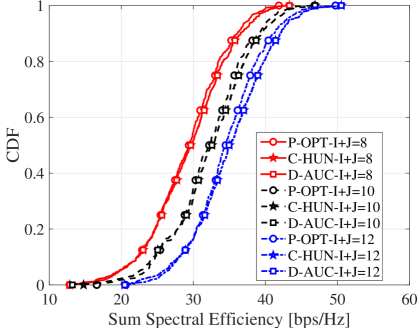
Figure 2: CDF of the optimality gap of the sum spectral efficiency for different users’ load. We notice that the optimality gap between the proposed D-AUC and the exhaustive search solutions of the primal and dual, E-OPT and C-HUN, is low, which suggests that we can use a distributed solution based on the dual and still be close to the centralized optimal solution of the primal.

We notice that the differences between the exhaustive search solutions, either E-OPT OR C-HUN, to the D-AUC is negligible, where in some cases the D-AUC achieves a higher performance than E-OPT due to lack of computational power to find the best powers. Figure 2 clearly shows that the optimality gap is low for the distributed auction when compared to the centralized dual solution (C-HUN) and also to the primal solution (E-OPT). Therefore, we can use a distributed solution to solve the primal problem (2) and still achieve a solution close to the centralized optimal solution.

Figure 3 shows the sum spectral efficiency between the current HD system, a naive FD implementation named R-EPA, and the proposed distributed solution D-AUC. We assume a small system fully loaded with 25 UL, DL users, and frequency channels, where we analyse the impact of the solutions for different SI cancelling levels of $-110\,\mathrm{dB}$ and $-70\,\mathrm{dB}$, i.e., $\beta=$$-110\,\mathrm{dB}$ and $-70\,\mathrm{dB}$.

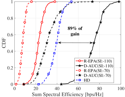
Figure 3: CDF of the sum spectral efficiency among all users for different SI cancelling levels. We notice that with $\beta=$$-110\,\mathrm{dB}$ the UE-to-UE interference is the limiting factor, where D-AUC mitigates this new interference and outperforms the HD mode and the R-EPA. When $\beta=$$-70\,\mathrm{dB}$, the SI is the limiting factor, where the mitigation of the UE-to-UE interference is not enough to bring gains to FD cellular networks.

Notice that with a SI cancelling level of $-110\,\mathrm{dB}$ we achieve $89\,\mathrm{\%}$ relative gain in the spectral efficiency at the 50th percentile, which is close to the expected doubling of FD networks. Moreover, the naive R-EPA performs approximately $43\,\mathrm{\%}$ worse than the HD mode, which shows that despite the high SI cancelling level, we do not have any gain of using FD networks. This behaviour shows that we should also optimize the UL-DL pairing and the power allocation of the UL user and of the BS. When the SI level is $-70\,\mathrm{dB}$, HD outperforms the D-AUC and R-EPA with a relative gain of approximately $23\,\mathrm{\%}$ and $81\,\mathrm{\%}$ at the 50th percentile, respectively. This means that with low SI cancelling levels the D-AUC algorithm is not able to overcome the high self-interference, although the difference to HD is not high. As for the R-EPA, notice that its performance is even worse than before, which once more indicates that we should not use naive implementation of user pairing and power allocation on FD cellular networks. Overall, we notice that when the SI cancelling level is high, the UE-to-UE interference is the limiting factor, where our proposed D-AUC outperforms a naive FD implementation that disregards this interference. When the SI cancelling level is low, then the SI is the limiting factor, where optimizing the UE-to-UE interference is not enough to bring gains to FD cellular networks.

VI Conclusion

In this paper we considered the joint problem of user pairing and power allocation in FD cellular networks. Specifically, our objective was to maximize the weighted sum spectral efficiency of the users, where we can tune the weights to sum maximization or path loss compensation. This problem was posed as a mixed integer nonlinear optimization, which is hard to solve directly, thus we resorted to Lagrangian duality and developed a closed-form solution for the assignment and optimal power allocation. Since we were interested in a distributed solution between the BS and the users, we proposed a novel distributed auction solution to solve the assignment problem, whereas the power allocation was solved in a centralized manner. We showed that the distributed auction converges and that it has a guaranteed performance compared to the dual. The numerical results showed that our distributed solution drastically improved the sum spectral efficiency in a path loss compensation modelling, i.e. of the users with low spectral efficiency, when compared to current HD modes when the SI cancelling level is high. Furthermore, we noticed that with a high SI cancelling level, the impact of the UE-to-UE interference is severe and needs to be properly managed. Conversely, when the SI cancelling level is low, a proper management of the UE-to-UE interference is not enough to bring gains to FD cellular networks. Studying the case of asymmetric assignment, that is the case of unequal number of UL and DL users and the impact of the number of iterations and processing delays in the auction algorithm are left for future works.

References

- [1] M. Heino, D. Korpi et al., “Recent Advances in Antenna Design and Interference Cancellation Algorithms for In-Band Full Duplex Relays,” IEEE Communications Magazine, vol. 53, no. 5, pp. 91–101, May 2015.
- [2] L. Laughlin, M. A. Beach et al., “Electrical Balance Duplexing for Small Form Factor Realization of In-Band Full Duplex,” IEEE Communications Magazine, vol. 53, no. 5, pp. 102–110, May 2015.
- [3] D. Bharadia, E. McMilin, and S. Katti, “Full Duplex Radios,” SIGCOMM Comput. Commun. Rev., vol. 43, no. 4, pp. 375–386, Oct. 2013.
- [4] K. Thilina, H. Tabassum et al., “Medium Access Control Design for Full Duplex Wireless Systems: Challenges and Approaches,” IEEE Communications Magazine, vol. 53, no. 5, pp. 112–120, May 2015.
- [5] S. Goyal, P. Liu et al., “Full Duplex Cellular Systems: Will Doubling Interference Prevent Doubling Capacity ?” IEEE Communications Magazine, vol. 53, no. 5, pp. 121–127, May 2015.
- [6] A. Osseiran, F. Boccardi et al., “Scenarios for 5G mobile and wireless communications: the vision of the METIS project,” IEEE Communications Magazine, vol. 52, no. 5, pp. 26–35, May 2014.
- [7] J. Bai and A. Sabharwal, “Distributed full-duplex via wireless side-channels: Bounds and protocols,” IEEE Transactions on Wireless Communications, vol. 12, no. 8, pp. 4162–4173, Aug. 2013.
- [8] C. Nam, C. Joo, and S. Bahk, “Joint Subcarrier Assignment and Power Allocation in Full-Duplex OFDMA Networks,” IEEE Transactions on Wireless Communications, vol. 14, no. 6, pp. 3108–3119, Jun. 2015.
- [9] M. Feng, S. Maoa, and T. Jiang, “Joint Duplex Mode Selection, Channel Allocation, and Power Control for Full-Duplex Cognitive Femtocell Networks,” Digital Communications and Networks, vol. 1, no. 1, pp. 30–44, Apr. 2015.
- [10] A. Simonsson and A. Furuskar, “Uplink power control in LTE - overview and performance,” in Proc. of the IEEE Vehic. Tech. Conf. (VTC), 2008.
- [11] A. Gjendemsjø, D. Gesbert et al., “Binary power control for sum rate maximization over multiple interfering links,” IEEE Transactions on Wireless Communications, vol. 7, no. 8, pp. 3164–3173, Aug. 2008.
- [12] D. Feng, L. Lu et al., “Device-to-Device Communications Underlaying Cellular Networks,” IEEE Transactions on Communications, vol. 61, no. 8, pp. 3541–3551, Aug. 2013.
- [13] R. E. Burkard and E. Çela, “Linear Assignment Problems and Extensions,” in Handbook of Combinatorial Optimization, D.-Z. Du and P. M. Pardalos, Eds. Springer US, 1999, pp. 75–149.
- [14] D. P. Bertsekas, Network Optimization: Continuous and Discrete Models. Cambridge, MA: MIT Press, 1998.
- [15] 3GPP, “Evolved Universal Terrestrial Radio Access (E-UTRA) and Evolved Universal Terrestrial Radio Access Network (E-UTRAN); Overall description; Stage 2,” 3rd Generation Partnership Project (3GPP), TS 36.300, Sep. 2015.
- [16] Y. Xu, “Decentralized Network Optimization in Wireless Networks,” pp. viii, 112, 2014.
- [17] 3GPP, “Evolved Universal Terrestrial Radio Access (E-UTRA); Further advancements for E-UTRA physical layer aspects,” 3rd Generation Partnership Project (3GPP), TR 36.814, Mar. 2010.