The crowded magnetosphere of the post common envelope binary QS Virginis

Abstract

We present high speed photometry and high resolution spectroscopy of the eclipsing post common envelope binary QS Virginis (QS Vir). Our UVES spectra span multiple orbits over more than a year and reveal the presence of several large prominences passing in front of both the M star and its white dwarf companion, allowing us to triangulate their positions. Despite showing small variations on a timescale of days, they persist for more than a year and may last decades. One large prominence extends almost three stellar radii from the M star. Roche tomography reveals that the M star is heavily spotted and that these spots are long-lived and in relatively fixed locations, preferentially found on the hemisphere facing the white dwarf. We also determine precise binary and physical parameters for the system. We find that the $14,220\pm 350$ K white dwarf is relatively massive, $0.782\pm 0.013$$\mathrm{M_{\odot}}$, and has a radius of $0.01068\pm 0.00007$$\mathrm{R_{\odot}}$, consistent with evolutionary models. The tidally distorted M star has a mass of $0.382\pm 0.006$$\mathrm{M_{\odot}}$ and a radius of $0.381\pm 0.003$$\mathrm{R_{\odot}}$, also consistent with evolutionary models. We find that the magnesium absorption line from the white dwarf is broader than expected. This could be due to rotation (implying a spin period of only $\sim$700 seconds), or due to a weak ($\sim$100kG) magnetic field, we favour the latter interpretation. Since the M star’s radius is still within its Roche lobe and there is no evidence that its over-inflated we conclude that QS Vir is most likely a pre-cataclysmic binary just about to become semi-detached.

1 Introduction

Close binaries containing a white dwarf and a low-mass M star are survivors of a common envelope phase of evolution during which both stars orbited within a single envelope of material ejected by the progenitor of the white dwarf. These systems slowly lose angular momentum via gravitational radiation and (if the M star is massive enough) magnetic braking, eventually becoming semi-detached cataclysmic variable (CV) systems.

Table 1: Journal of observations. The eclipse of the white dwarf occurs at phase 1, 2 etc.

Date at	Instrument	Telescope	Filter(s)	Start	Orbital	Exposure	Number of	Conditions
start of run				(UT)	phase	time (s)	exposures	(Transparency, seeing)
2002/05/20	ULTRACAM	WHT	$u^{\prime}g^{\prime}r^{\prime}$	20:51	0.48–1.55	1.1	10533	Fair, $\sim$2 arcsec
2003/05/20	ULTRACAM	WHT	$u^{\prime}g^{\prime}i^{\prime}$	23:43	0.93–1.64	2.9	1983	Variable, 1.2-3 arcsec
2003/05/22	ULTRACAM	WHT	$u^{\prime}g^{\prime}i^{\prime}$	00:39	0.84–1.10	2.9	957	Good, $\sim$1.5 arcsec
2003/05/24	ULTRACAM	WHT	$u^{\prime}g^{\prime}i^{\prime}$	22:02	0.38–1.07	2.9	2233	Good, $\sim$1.2 arcsec
2006/03/13	ULTRACAM	WHT	$u^{\prime}g^{\prime}r^{\prime}$	00:42	0.88–1.09	2.4	1098	Fair, $\sim$2 arcsec
2010/04/21	ULTRACAM	NTT	$u^{\prime}g^{\prime}i^{\prime}$	06:35	0.88–1.37	1.7	3665	Good, $\sim$1.2 arcsec
2011/01/07	ULTRACAM	NTT	$u^{\prime}g^{\prime}i^{\prime}$	08:08	0.89–1.09	1.9	1409	Good, $\sim$1.3 arcsec
2011/05/29	ULTRACAM	NTT	$u^{\prime}g^{\prime}r^{\prime}$	04:49	0.92–1.08	3.9	550	Poor, $\sim$1.5 arcsec
2013/05/05	UVES	VLT	-	00:10	0.28–2.04	180.0	98	Excellent, $<$1 arcsec
2013/05/05	UVES	VLT	-	23:52	0.83–2.15	180.0	74	Excellent, $<$1 arcsec
2014/04/24	UVES	VLT	-	03:01	0.21–1.30	180.0	62	Good, $\sim$1.0 arcsec
2014/04/25	UVES	VLT	-	02:19	0.65–1.74	180.0	62	Good, $\sim$1.0 arcsec
2014/05/01	UVES	VLT	-	02:04	0.38–1.51	180.0	62	Good, $\sim$1.3 arcsec
2014/05/31	UVES	VLT	-	23:30	0.29–1.39	180.0	62	Excellent, $<$1 arcsec

In recent years the number of such systems known has dramatically increased, thanks mainly to the Sloan Digital Sky Survey (SDSS, York et al. 2000; Adelman-McCarthy et al. 2008; Abazajian et al. 2009), which has lead to the discovery of more than 2000 white dwarf plus main-sequence systems (Rebassa-Mansergas et al., 2013a), from which more than 200 close, post common-envelope binaries (PCEBs) have been identified (Nebot Gómez-Morán et al., 2011; Parsons et al., 2013b, 2015). Among this sample are 71 eclipsing binaries (see the appendix of Parsons et al. 2015 for a recent census). These are extremely useful systems for high precision stellar parameter studies, since the small size of the white dwarf leads to very sharp eclipse profiles, allowing radius measurements to a precision of better than two per cent (e.g. Parsons et al., 2010a), good enough to test models of stellar and binary evolution.

The main-sequence star components in PCEBs are tidally locked to the white dwarf and hence are rapidly rotating. This rapid rotation results in very active stars. Indeed, it appears as though virtually every PCEB hosts an active main-sequence star, regardless of its spectral type (Rebassa-Mansergas et al., 2013b). Even extremely old systems still show signs of activity (Parsons et al., 2012b), manifesting as starspots and flaring. These features allow us to constrain the configuration of the underlying magnetic field of the main-sequence star, crucial for understanding the evolution of these binaries, since the magnetic field is able to remove angular momentum from the system, driving the two stars closer together (Rappaport et al., 1983; Kawaler, 1988).

Discovered as an eclipsing PCEB by O’Donoghue et al. (2003), QS Vir (EC 13471$-$1258) has been intensely studied since it shows signs of being both a standard pre-CV, detached white dwarf plus main-sequence binary (Ribeiro et al., 2010; Parsons et al., 2011), as well as indications of accretion of material on to the white dwarf well above standard rates for detached systems (Matranga et al., 2012); the M star is also very close to filling its Roche lobe, leading to the initial interpretation that it could in fact be a hibernating CV that has recently detached due to a nova eruption (O’Donoghue et al., 2003). Furthermore, the arrival times of its eclipse show substantial variations (Parsons et al., 2010b), which some authors have claimed may be due to the gravitational effects of circumbinary planets (Almeida & Jablonski, 2011), although the proposed orbital configuration has recently been shown to be highly unstable (Horner et al., 2013), meaning that the true origin of these variations remains unexplained.

The M star in QS Vir is very active, indicated both by evidence of substantial flaring (Parsons et al., 2010b), as well as intriguing narrow absorption features detected in high resolution spectra by Parsons et al. (2011). This absorption was found to be due to material expelled from the M star passing in front of the white dwarf. In this paper we investigate the behaviour of the material lost by the M star and its motion within the binary over a time span of more than a year as well as performing Roche tomography to identify and track starspots on the surface of the M star. We also place stringent constraints on the stellar and binary parameters.

2 Observations and their reduction

In this section we outline our observations and their reduction. A full log of all our observations is given in Table 1.

2.1 ULTRACAM photometry

QS Vir has been observed many times with the high speed frame-transfer camera ULTRACAM (Dhillon et al., 2007). These observations date back to 2002 and were obtained with ULTRACAM mounted as a visitor instrument on the 4.2-m William Herschel Telescope (WHT) on La Palma and the 3.5-m New Technology Telescope (NTT) on La Silla. Much of these data were presented in Parsons et al. (2010b), however, we detail both the older data and our new data in Table 1. ULTRACAM uses a triple beam setup allowing one to obtain data in the $u^{\prime}$, $g^{\prime}$ and either $r^{\prime}$ or $i^{\prime}$ band simultaneously.

All of these data were reduced using the ULTRACAM pipeline software. Debiassing, flatfielding and sky background subtraction were performed in the standard way. The source flux was determined with aperture photometry using a variable aperture, whereby the radius of the aperture is scaled according to the full width at half maximum (FWHM). Variations in observing conditions were accounted for by determining the flux relative to a comparison star in the field of view. The data were flux calibrated using observations of standard stars observed during twilight.

2.2 UVES spectroscopy

We observed QS Vir with the high resolution Echelle spectrograph UVES (Dekker et al., 2000) installed at the European Southern Observatory Very Large Telescope (ESO VLT) 8.2-m telescope unit on Cerro Paranal. We used the dichroic 2 setup allowing us to cover 3760Å–4990Å in the blue arm and 5690Å–9460Å in the red arm, with a small gap between 7520Å and 7660Å and 2x2 binning in both arms. We used exposure times of 3 minutes in order to reduce the effects of orbital smearing, this gives a signal-to-noise ratio in the continuum ranging from $\sim$15 at the shortest wavelengths to $\sim 40$ at longer wavelengths.

Our data consist of two separate observing runs. The first, in 2013, was conducted in visitor mode over two nights. On each night we covered well over a full orbital period. During this run we also observed several M star spectral type standards covering the range M3.0 to M4.5. The second run comprised of a series of four service mode observations made over a month roughly a year after our visitor mode observations. Each of these observations covered just over an orbital period.

All the data were reduced using the most recent release of the UVES data reduction pipeline (version 5.3.0). The standard recipes were used to optimally extract each spectrum. We used observations of the featureless DC white dwarf LHS 2333 to flux calibrate and telluric correct our spectra.

3 Results

3.1 Spectrum

The spectrum of QS Vir was first described by O’Donoghue et al. (2003). Ribeiro et al. (2010) and Parsons et al. (2011) also presented higher resolution spectra. Both components of the binary are clearly visible in the spectrum, with the Balmer lines of the white dwarf the dominant features at wavelengths less than $\sim$5000Å and the molecular absorption features of the M star the dominant features at longer wavelengths. There are also several emission lines originating from the M star throughout the spectrum caused by a combination of activity and irradiation from the white dwarf. As noted by Parsons et al. (2011) there is also a weak Mg ii 4481Å absorption line from the white dwarf.

Figure 1: UVES blue arm spectrum of QS Vir taken at an orbital phase of $\phi=0.22$ showing sharp absorption features from material passing in front of the white dwarf. Emission lines are also present originating from the M star component caused by a combination of activity and irradiation.

In addition to these general features, we also re-detect the narrow absorption features noted by Parsons et al. (2011) in the hydrogen Balmer series and calcium H and K lines, an example of this is shown in Figure 1. Furthermore, we also detect absorption features in several other species including the sodium D lines and several Mg i and Fe ii lines. The behaviour and origin of these features are discussed in the following section.

3.2 Prominence features

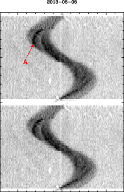
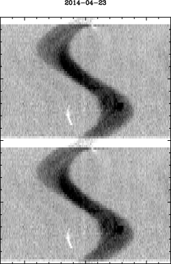
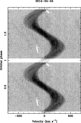
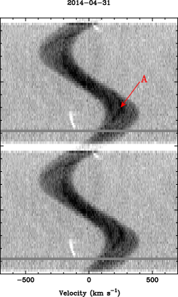
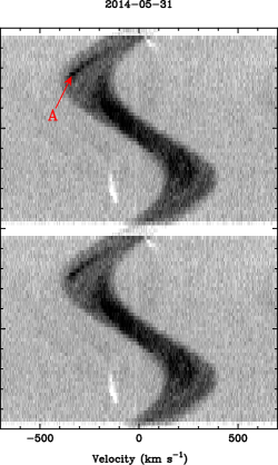
Figure 2: Phase-folded trailed spectrograms of the Ca ii 3934Å line, data shown twice for visual continuity. The date at the start of the night the data were obtained is shown above each plot. Higher fluxes are darker. The main features visible are the emission from the active M star and the eclipse of the white dwarf. However, a narrow absorption feature is visible just before and after the eclipse (“B”) and at phase 0.25 (“C”) in all the plots. This is caused by material moving in front of the white dwarf and, although variable, is always visible, despite the data spanning more than a year.

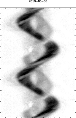
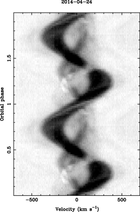
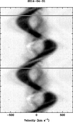
Figure 3: Phase-folded trailed spectrograms of the H$\alpha$ line, data shown twice for visual continuity. The continuum has been subtracted from each spectrum and the date at the start of the night the data were obtained is shown above each plot. Higher fluxes are darker. The strongest component is emission from the active M star. However, there are at least two other emission components (“E”), neither of which originate from either of the stars. Material is seen moving across the face of both the white dwarf (“C”) and M star (“D”). Despite being separated by more than a year, the trails look remarkably similar.

The sharp absorption features detected by Parsons et al. (2011) were attributed to a prominence from the M star passing in front of the white dwarf. However, only a single spectrum was available, limiting the constraints that could be placed on its location and size. Our new data cover the full binary orbit and hence much tighter constraints can be placed. Moreover, our data cover multiple orbits over a timescale of more than a year, allowing us to investigate the evolution of these features. Figure 2 shows trailed spectrograms of the Ca ii 3934Å line on 6 separate nights, covering timescales from a day to a year. Strong emission from the M star is visible resulting from a combination of activity and irradiation (note how the emission is strongest at phase 0.5, when the irradiated face points towards us). There are additional short-lived localised emission components from the M star labelled “A” in Figure 2, best seen in the 5th of May 2013 data (middle-top panel of Figure 2). These narrow emission features occur on top of the intrinsic emission from the M star and only persist for single orbits, they are likely related to flares on its surface. There is also a narrow non-variable, zero velocity absorption component likely the result of interstellar absorption.

In addition to emission from the M star, there is also a narrow absorption line moving in anti-phase to the M star, but only visible at certain orbital phases. This absorption is seen just before and after the eclipse of the white dwarf (labelled “B” in Figure 2, particularly clear in the 2013 data) as well as close to phase 0.25, labelled “C”. When visible, these absorption features have the same velocity as the white dwarf (see Section 3.3), implying that this material blocking the light of the white dwarf has no radial velocity relative to it, and suggests that it is in a state of solid-body rotation with respect to the binary, likely in the form of prominences.

The most striking aspect of Figure 2 is that these prominence features appear to persist on timescales of days, weeks, months and years. Given the similarity of the prominence feature detected at on orbital phase of 0.16 in the 2002 spectra by Parsons et al. (2011), it also appears that these features could be stable on timescales of decades. However, Figure 2 also shows that they are not completely fixed. The absorption feature around phase 0.25 is visible for longer during 2014 compared to the 2013 data. Meanwhile the absorption around the eclipse is much clearer in the 2013 data and is only obvious before the eclipse in the 2014 dataset.

In Figure 3 we show the same plots as Figure 2 but for the H$\alpha$ line. This line shows a much more complex behaviour, with multiple absorption and emission components visible. The strongest component is still the emission from the M star, but narrow absorption components are seen crossing this emission throughout the orbit during all six observations (the strongest are labelled “D” in Figure 3). The prominence material passing in front of the white dwarf is still visible (“C”), albeit slightly weaker than in the Ca ii line since the white dwarf contributes a smaller amount of the overall flux at H$\alpha$. Furthermore, there are several additional emission components which do not correspond to either star in the binary, labelled “E”. The H$\alpha$ line also shows considerable variability in the strength of all these features from night-to-night compared to the Ca ii line.

In Figure 4 we show a larger version of the Ca ii and H$\alpha$ trailed spectrogram from the second observing run (5th of May 2013) with some of the major features labelled. The radial velocity of the white dwarf and M star are shown as red lines (see Section 3.3 and 3.4). We highlight in blue three clear prominence-like absorption features visible in all six observations, that appear to cross one or both of the stars. In addition we highlight three additional emission components visible in the H$\alpha$ trail that do not originate from either star.

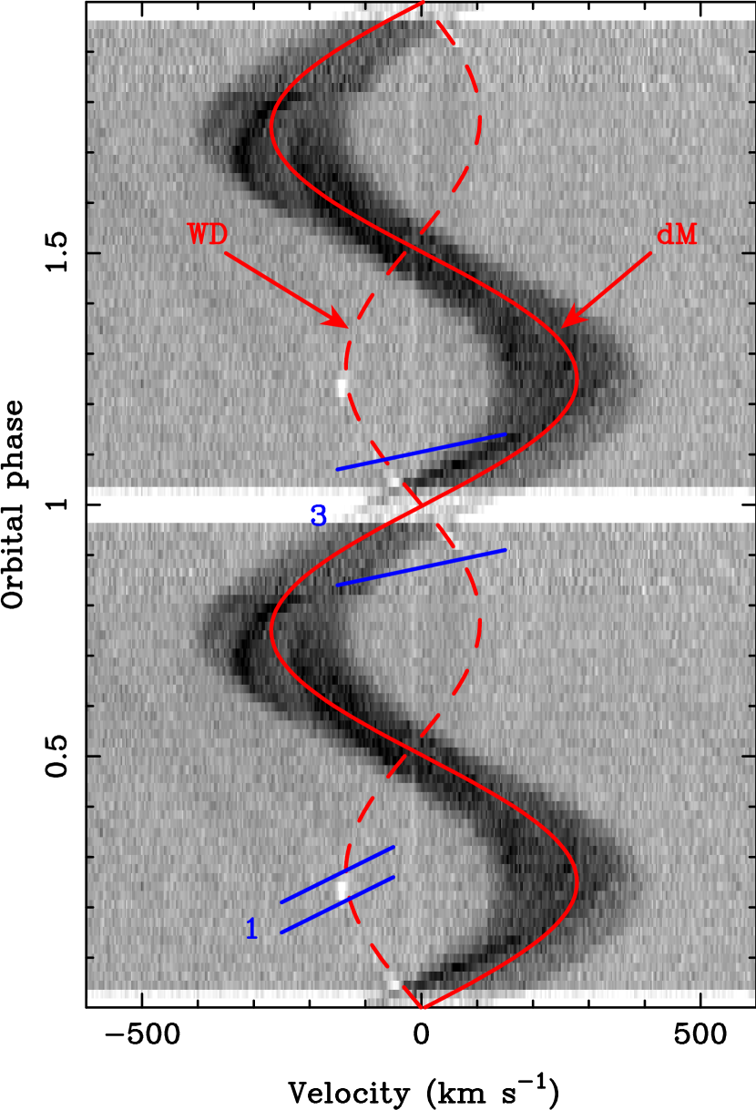
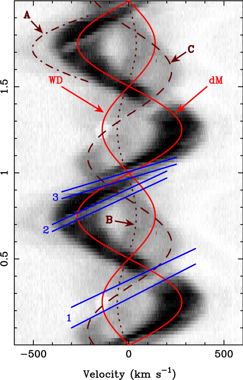
Figure 4: Trailed spectrogram of the Ca ii 3934Å (left) and H$\alpha$ (right) lines from 5th May 2013 with the main features labelled. The velocities of the two stars are indicated by the bright red sinusoids. In blue we highlight three clear absorption features that cross one of both of the stars (only two are visible in the Ca ii trail). We also highlight three other emission components in the H$\alpha$ trail with dark red lines.

To further highlight the various emission components visible in the trailed spectrogram of the H$\alpha$ line we used Doppler tomography (Marsh & Horne, 1988). We used the MODMAP code described in Steeghs (2003) to reconstruct the Doppler map shown in Figure 5, using all the data from May 5th 2013. It clearly shows that the strongest emission component originates from the M star itself, but the three additional emission components visible in the trailed spectrogram are seen more clearly, with two close to the white dwarf’s Roche lobe and one high velocity emission component. These components are labelled “A”, “B” and “C” and correspond to the additional emission seen in the H$\alpha$ trail in Figure 4, where we have used the same labels to highlight the features.

Figure 5: Doppler map of the H$\alpha$ line from 5th May 2013. The Roche lobes of the white dwarf and M star are highlighted with a black dashed line and solid white line respectively. To highlight the additional emission features against the strong emission from the M star we have also plotted contours. Three clear emission features that do not originate from either star are labelled.

The clearest prominence feature in Figure 4, labelled “1”, is responsible for the narrow absorption line seen at around phase 0.25 in the Ca ii line, when it passes in front of the white dwarf. At around phase 0.4 this same material passes in front of the M star, completely blocking the H$\alpha$ emission component from this star. Furthermore, this prominence is seen in emission at certain orbital phases, highlighted as component “C” in both Figure 4 and Figure 5. It is possible that the prominence is dense enough that it is able to reprocess the light it receives from the white dwarf. Alternatively, this could be intrinsic emission from the prominence. Figure 3 shows that the strength of this emission clearly varied from 2013 to 2014, weakening in 2014.

The fact that this prominence crosses in front of both stars allows us to triangulate its position within the binary. Figure 6 shows a visualisation of the binary indicating both the location and size of this prominence. We show this for both 2013 and 2014, variations on shorter timescales are minimal. As is evident from Figures 2 and 3 the prominence is larger in 2014, clearly taking longer to pass in front of the white dwarf. We also show the viewing angle to the white dwarf in the 2002 data from Parsons et al. (2011) which also passed through a similar prominence feature.

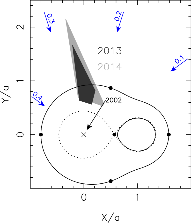
Figure 6: A top down view of the binary indicating the location of the large prominence feature in 2013 and 2014 (feature “1” in Figure 4), the stars rotate clockwise and the viewing angle to the white dwarf at various orbital phases is shown in blue. The dotted lines indicate the Roche lobes of the two stars, the radius of the M star is shown as a solid line. The arrow indicates the viewing angle to the white dwarf during the 2002 observation from Parsons et al. (2011) in which prominence material was also observed. The cross marks the location of the white dwarf and the black points indicate the location of the five Lagrange points. The outer solid black line indicates the effective “co-rotation” radius of the binary (see the text for a definition of this radius).

The stability and longevity of this feature is remarkable, given that it is located at an unstable location within the binary and hence the material should be expelled quickly. In Figure 6 we plot the effective “co-rotation” radius of the binary. While this radius is well defined for a single star (the radius at which the gravitational attraction equals the centripetal acceleration of a particle in solid-body rotation with the star, hence a particle can sit there with no other force needed to hold it), such a radius does not exist for a binary. In this case the centripetal acceleration acts towards the centre of mass, but the gravitational forces act towards the two stars and so there is not a stable radius, but rather five equilibrium points (the Lagrangian points). However, in Figure 6 we slightly extend the definition by considering the radial component of acceleration in the rotating frame (automatically including gravity and centripetal terms) as measured from the centre of mass of the M star, resulting in a line that passes through the Lagrangian points. Nevertheless, except for at the Lagrangian points themselves, there are still forces acting perpendicular to this line, so it does not represent a stable region within the binary, hence some additional force is required to keep material in this region. However, it may well be easier for material to stay fixed near this line than at other locations. From Figure 6 it is evident that material is located at this radius, but also extends substantially beyond it, requiring that quite significant non-gravitational forces are acting upon it (presumably some sort of magnetic force).

The feature labelled “2” in Figure 4 crosses the M star at an orbital phase of $\sim$0.75, but does not appear to pass in front of the white dwarf (hence it is not visible in the Ca ii trail), meaning that we cannot completely determine its location or size like the large prominence. It is possible that it passes in front of the white dwarf shortly before or during the eclipse, in which case it would be located close to the surface of the M star. Or instead, this particular prominence could be at an inclination such that it only passes in front of the M star. This prominence weakened considerably between 2013 and 2014 and is barely visible in the last observations in Figure 3. There does not appear to be an obvious emission component associated with this prominence.

The feature labelled “3” in Figure 4 crosses the face of the M star during the eclipse of the white dwarf, and therefore this material must be located behind the M star, from the white dwarf’s perspective. Moreover, the Ca ii trail shows that this material also passes in front of the white dwarf just before and after the eclipse. Unfortunately, this means that we cannot determine the exact location of this material either. This prominence is seen in emission as a high velocity component blueward of the M star at phase 0.75 (labelled “A”) in the H$\alpha$ trail (dot-dashed line) and more clearly at (-650,450) in Figure 5. Similar absorption features were detected in ultraviolet spectra of V471 Tau just before and after the eclipse of the white dwarf (Guinan et al., 1986), which they attributed to cool coronal loops. Interestingly, O’Donoghue et al. (2003) detected a sharp pre-eclipse dip in the light curve of QS Vir (see their Figure 8) which could be from similar coronal loops, implying that this material can sometimes be dense enough to block out continuum light. However, the lack of a comparison star during this observation means that this dip should be interpreted with some caution. Despite our extensive photometric monitoring (e.g. Table 1) this dip has not been seen since.

Finally, there is another emission component highlighted in the H$\alpha$ trail in Figure 4 by a dotted line (labelled “B”). It moves in anti-phase with the M star, but with a much lower velocity than the white dwarf, meaning that this must originate from material between the two stars. It is also visible in Figure 5 close to (0,0), within the Roche lobe of the white dwarf. Figure 3 shows that this emission was much stronger in 2014 compared to 2013. Assuming that this material co-rotates with the binary, its location is given by

$$\frac{K_{\mathrm{mat}}}{K_{\mathrm{sec}}}=(1+q)\left(\frac{R}{a}\right)-q,$$ (1)

where $K_{\mathrm{mat}}$ and $K_{\mathrm{sec}}$ are the radial velocity semi-amplitudes of the material and the M star respectively, $q$ is the mass ratio and $R/a$ is the distance of the material from the white dwarf scaled by the orbital separation ($a$).

Using our measured values of $K_{\mathrm{sec}}$ and $q$ (see Sections 4 and 5) and $K_{\mathrm{mat}}=-100$$\mathrm{km\,s^{-1}}$determined by Gaussian fitting in the same way as outlined in the next section, gives $R/a=0.09$. Similar emission features have been seen in other post common-envelope binaries (Parsons et al., 2013a; Tappert et al., 2011) as well as CVs (Steeghs et al., 1996; Gänsicke et al., 1998; Kafka et al., 2005, 2006) and could be related to another prominence structure or heated material from the wind of the M star close to the white dwarf. Interestingly, there appears to be a genuine deficiency of H$\alpha$ emission from the inner face of the M star, best seen in Figure 5. The deficiency may be due to this material between the two stars shielding the M star from irradiation by the white dwarf.

Despite being an eclipsing system, the inclination of QS Vir is relatively low ($i=77.7^{\circ}$, see Section 5), therefore, not only are these prominences far from the M star, they are also located far from its equatorial plane. However, many cool, isolated low-mass stars show similar prominence systems beyond their co-rotation radii (Donati et al., 1999; Dunstone et al., 2006), and located far from their equatorial planes (Collier Cameron & Robinson, 1989). Indeed, Jardine et al. (2001) found that for single stars there exist stable locations both inside and outside the co-rotation radius and up to 5 stellar radii from the star (Jardine & van Ballegooijen, 2005). Long-lived prominences have also been detected in the CVs BV Cen (Watson et al., 2007), IP Peg and SS Cyg (Steeghs et al., 1996) and AM Her (Gänsicke et al., 1998). Magnetically confined material was also detected in BB Dor (Schmidtobreick et al., 2012) and near the L4 and L5 Lagrange points in AM Her (Kafka et al., 2008). In addition, the detached white dwarf plus main-sequence star binaries V471 Tau (Jensen et al., 1986) and SDSS J1021+1744 (Irawati et al., 2016) both show long-lived prominence-like features, in very similar positions to the large prominence in QS Vir.

3.3 White dwarf radial velocity amplitude

We measure the radial velocity amplitude of the white dwarf using the narrow Mg ii 4481Å absorption line. Due to emission from the M star, the cores of the hydrogen Balmer lines are not visible, thus making them unsuitable for radial velocity work. No other intrinsic white dwarf absorption features are detected in the UVES spectra.

We fit the Mg ii line in each spectrum with a combination of a straight line and a Gaussian component. We do not fit the spectra obtained whilst the white dwarf was in eclipse (including the ingress and egress phases). Furthermore, we do not fit the spectra taken during phases 0.45–0.55, since during these phases Mg ii emission from the heated inner hemisphere of the M star fills in the absorption as the two components cross over. The resultant velocity measurements and their corresponding orbital phases were then fitted with a sinusoid to determine the white dwarf’s radial velocity semi-amplitude. The result of this is shown in Figure 7. We find a radial velocity semi-amplitude for the white dwarf of $139.0\pm 1.0$$\mathrm{km\,s^{-1}}$, with a mean velocity of $43.2\pm 0.8$$\mathrm{km\,s^{-1}}$, consistent with (but much more precise than) the measurement from O’Donoghue et al. (2003) ($137\pm 10$$\mathrm{km\,s^{-1}}$and $61\pm 10$$\mathrm{km\,s^{-1}}$ respectively) using Hubble Space Telescope (HST) spectra, although our mean velocity is a little lower than their measured value. The mean velocity of the white dwarf is redshifted from the systemic velocity of the binary due to its high gravity, which can be used to constrain its physical parameters (see Section 5).

Figure 7: Radial velocity measurements of the Mg ii 4481Å absorption line from the white dwarf with fit (red line). The residuals of the fit are shown in the bottom panel.

3.4 M star radial velocity amplitude

We attempted to measure the radial velocity semi-amplitude of the M star using the same technique outlined in the last section (i.e. a Gaussian fit) and fitting the Na i 8200Å absorption doublet. Figure 8 shows the result of this fit. At first glance it seems that the semi-amplitude is tightly constrained by the data (the average uncertainty on an individual velocity measurement is $\sim$1$\mathrm{km\,s^{-1}}$). However, as the residuals show, the deviation from a pure sinusoid are quite pronounced and there are clearly large systematic trends affecting the velocity measurements. These deviations are seen in the data from both 2013 and 2014 as well as for other atomic features, such as the K i 7665Å and 7699Å lines. Therefore, we do not consider these measurements a true representation of the centre-of-mass velocity of the M star.

The most likely cause of this deviation is the presence of starspots on the surface of the M star, although gravity darkening and irradiation may also contribute to this. Therefore, in order to determine a more reliable value for the radial velocity semi-amplitude for the M star, as well as a better understanding of the starspot distribution and evolution, we used our UVES spectra to perform Roche tomography of the M star, which we detail in the following section.

4 Roche tomography

Roche tomography is a technique analogous to Doppler imaging (e.g. Vogt & Penrod, 1983), and has been successfully used to image surface features on the secondary stars in interacting binaries. The technique assumes the secondary star rotates synchronously in a circular orbit around the centre of mass, and uses phase-resolved spectral line profiles to map the line-intensity distribution across the star’s surface in real space. The method has been extensively applied to the secondary stars in CVs over the last 20 years (Rutten & Dhillon, 1994, 1996; Watson et al., 2003; Schwope et al., 2004; Watson et al., 2006, 2007; Hill et al., 2014), and artefacts arising from systematic errors are well characterised and understood. For a detailed description of the methodology and axioms of Roche tomography, we refer the reader to the references above and the technical reviews by Watson & Dhillon (2001) and Dhillon & Watson (2001).

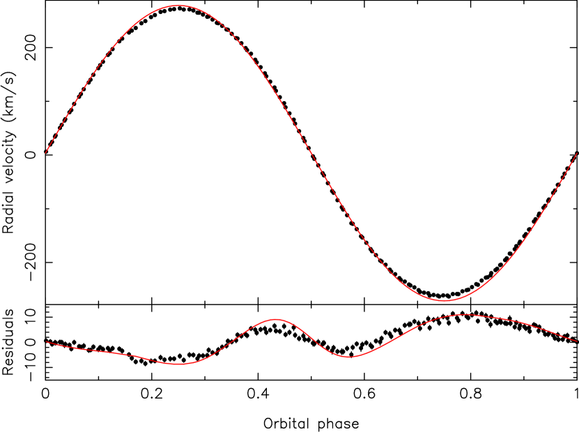
Figure 8: Radial velocity measurements of the Na i 8200Å absorption doublet from the M star using a Gaussian fit from the 2013 observations. The red line in the top panel is the centre-of-mass radial velocity of the M star determined from our Roche tomography analysis (see Section 4). Clear deviations from this fit are seen in the residuals in the lower panel as a result of the large number of star spots. The red line in the lower panel shows the deviations from the centre-of-light to the centre-of-mass radial velocity as determined from our Roche tomography analysis of the 2013 data, and show a very similar behaviour to the Gaussian measurements.

4.1 Least squares deconvolution

Spot features appear in absorption line profiles as an emission bump (actually a lack of absorption), and are typically a few per cent of the line depth. Thus, very high signal-to-noise ratio (SNR) data are required for surface imaging, a feat not directly achievable for a single absorption line with QS Vir due to its faintness and the requirements for short exposures to avoid orbital smearing. To greatly improve our SNR we employ least squares deconvolution (LSD), a technique that stacks the thousands of stellar absorption lines observable in a spectrum to produce a single ‘mean’ profile. First applied by Donati et al. (1997), the technique has been widely used since (e.g. Barnes et al., 2004; Shahbaz & Watson, 2007). For a more detailed description of LSD, we refer the reader to the above references as well as the review by Collier Cameron (2001).

To generate the LSD line profiles the continuum must be flattened. However, the contribution of the M star to the total system luminosity may vary due to variations in accretion luminosity (see Section 6.3), and the rapid flaring on the M star on timescales of several minutes (O’Donoghue et al., 2003). Both of these mechanisms may change the continuum slope, and so a master continuum fit to the data is not appropriate. Furthermore, normalization of the continuum would result in the photospheric absorption lines from the secondary varying in relative strength between exposures. This forces us to subtract the continuum from each spectrum, which was achieved by fitting a spline to the data.

To produce the LSD profiles we generated a line list appropriate for a M3.5V star ($\mathrm{T_{eff}}=3100\mathrm{K}$ and $\mathrm{log}g=4.88$) from the Vienna Atomic Line Database (VALD3; Kupka et al. 2000), adopting a detection limit of 0.1. The normalized line depths were scaled by a fit to the continuum of a M3.5V template star so each line’s relative depth was correct for use with the continuum subtracted spectra. As the transitions in molecular features (such as the prominent TiO bands) are difficult to model, the line lists for these features are of poor quality, and so we were unable to include spectral regions containing these features in LSD. In addition, we excluded emission lines and tellurics from the LSD process. Thus, a total of 46 absorption lines were used, lying in the spectral ranges $8400-8470$Å and $8585-8935$Å. As QS Vir is an eclipsing binary, there are significant features in the line profiles arising between phases 0.4–0.6 (superior conjunction) which do not originate on the secondary. As inclusion of these phases would cause artefacts to appear on the reconstructed maps (e.g. the entire inner hemisphere would appear to be irradiated), they were excluded from the fitting process. The LSD profiles were then binned on a uniform velocity scale of $7.4$$\mathrm{km\,s^{-1}}$ to match the velocity smearing due to the orbital motion.

The LSD profiles exhibited a clear continuum slope that was largely removed by subtracting a second-order polynomial fit to the continuum, preserving the profiles’ features and shape. However, these corrected profiles still exhibited a non-flat continuum which lay significantly below zero. To account for this, a constant offset was added to each set of LSD profiles, the specific value of which was non-trivial to determine due to degeneracies in the fitting process; if a small constant was added, a greater proportion of the line wings lay below the continuum, inflating the Roche lobe and changing the optimum masses found in the fit with Roche tomography. If a large constant was added, more of the line wings lay above the continuum, changing the optimum system parameters. Hence, an optimum value of constant to add to the LSD profiles could not be found computationally. Instead, the most appropriate offset was found by visual inspection of the fits to the data. This was done independently for each data set. These offset and continuum-flattened LSD profiles were then adopted for the rest of the fitting process with Roche tomography.

In general, Roche tomography cannot normally be performed on data which has not been corrected for slit losses, due to the secondary star’s variable light contribution. As the acquired data of QS Vir was largely photometric, we were able to correct for slit losses using an optimal-subtraction technique. Here, each LSD profile was scaled and subtracted from the fit made with Roche tomography, where the optimal scaling factor was that which minimized the residuals. The newly-scaled LSD profiles were then re-fit with Roche tomography, and the above process repeated until the scaling factors no longer varied. The resulting scaled profiles were visually inspected and found to be consistent. The final LSD profiles with computed fits and residuals are shown in Figure 9.

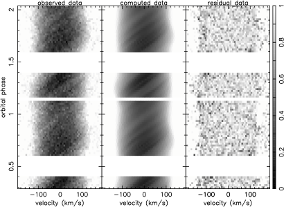
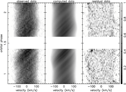
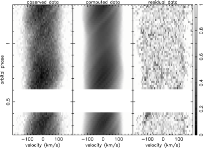
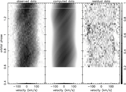
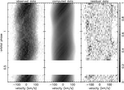
Figure 9: Trailed LSD profiles of QS Vir (2013-05-04 top left, 2013-05-05 top right, 2014-04-23 middle left, 2014-04-24 middle right, 2014-04-31 bottom left, 2014-05-31 bottom right). From left to right, panels show the observed LSD data, computed data from the Roche tomography reconstruction and the residuals (increased by a factor of 4). Starspot features in these panels appear bright. A grey-scale wedge is also shown, where a value of 0 corresponds to the maximum line depth in the reconstructed profiles. The orbital motion has been removed assuming the binary parameters found in Section 4.2, which allows the individual starspot tracks across the profiles and the variation in $V_{rot}\sin{i}$ to be more clearly observed.

4.2 System parameters

Roche tomography constrains the binary parameters by reconstructing intensity maps of the stellar surface for many combinations of $M_{1}$, $M_{2}$, inclination ($i$), systemic velocity ($\gamma$) and Roche-lobe filling factor (RLFF). Each map is fit to the same $\chi^{2}$. However, for a given value of $\chi^{2}$, many maps may fit the data equally well, and so the maximum-entropy regularisation statistic is employed for selecting the reconstructed map with least informational content required to fit the data (the most positive entropy value). Thus for any given set of parameters, the reconstructed map has an associated entropy. The optimal parameters are determined by selecting those that produce the map of maximum entropy across all possible parameter combinations. Adoption of incorrect system parameters results in the reconstruction of spurious artefacts in the final map (see Watson & Dhillon 2001 for details). Artefacts are well characterised and always increase the amount of structure mapped in the final image, which in turn leads to a decrease in the entropy regularisation statistic. All data sets were fit independently using this method.

It was assumed the rotation of the M dwarf is tidally locked to the orbital period, and so the period was fixed to 0.1507576116 d (Parsons et al., 2011). Additionally, the inclination was fixed to $i=77.8^{\circ}$, as this was well constrained from light-curve analysis – considering the SNR of the data being fit, we are unlikely to improve the accuracy of this using Roche tomography, and indeed an unsuccessful attempt was made to constrain inclination once optimal system parameters were found.

4.2.1 Limb Darkening

Roche tomography allows limb darkening to be included in the fitting of line profiles. In order to calculate the correct limb darkening coefficients, we determined the effective central wavelength of the data over ranges specified in Section 4.1 using,

$$\lambda_{\mathrm{cen}}=\frac{\sum_{i}\nolimits\frac{1}{\sigma_{i}^{2}}\>d_{i}\>\lambda_{i}}{\sum_{i}\nolimits\>\frac{1}{\sigma_{i}^{2}}\>d_{i}},$$ (2)

where $d_{i}$ is the line depth at wavelength $\lambda_{i}$, and $\sigma_{i}$ the error in the data at $\lambda_{i}$. The mean value of $\lambda_{cen}$ across the 6 datasets was used for consistency. We adopted a four-parameter non-linear limb darkening model (see Claret 2000), given by

$$\frac{I(\mu)}{I(1)}=1-\displaystyle\sum_{k=1}^{4}a_{k}(1-\mu^{\frac{k}{2}}),$$ (3)

where $\mu=\cos{\gamma}$ ($\gamma$ is the angle between the line of sight and the emergent flux), and $I(1)$ is the monochromatic specific intensity at the centre of the stellar disk.

Using the calculated $\lambda_{cen}$, the limb darkening coefficients were then determined by linearly interpolating between the tabulated wavelengths given in Claret (2000). We adopted stellar parameters closest to that of a M3.5V star, which for the PHOENIX model atmosphere were $\log{g}=5$ and $T_{\mathrm{eff}}=3100\mathrm{K}$. Thus, the adopted coefficients were $a_{1}=3.302,a_{2}=-5.057,a_{3}=4.612,a_{4}=-1.61$. We note that the limb darkening law used is for spherical stars, and so is not ideally suited to the distorted main-sequence star in QS Vir. Ideally one would need to calculate limb darkening coefficients for each tile in the grid based on a model atmosphere. However, this is not currently possible within our code, and so we adopted uniform limb darkening coefficients. Artefacts arising from adopting incorrect coefficients are discussed in Watson & Dhillon (2001).

4.2.2 Systemic velocity

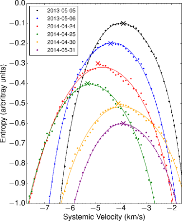
Figure 10: Points show the maximum entropy value obtained in each data set, as a function of systemic velocity. The optimal masses and RLFF as found in Section 4.2.3 were adopted for the fits of each data set. The points are plotted with a vertical offset of 0.1 between data sets. Crosses mark the value of $\gamma$ that yields the map of maximum entropy, and a sixth-order polynomial fit is shown as a visual aid. The mean systemic velocity across all data is $\gamma_{\mathrm{mean}}=-4.4_{-0.9}^{+0.5}$ kms^-1.

The entropy statistic is most sensitive to an incorrect systemic velocity $\gamma$, and so this parameter was narrowed down most easily. Figure 10 shows the map entropy yielded for each data set as a function of $\gamma$, where a cross marks the $\gamma$ that gives the map of maximum entropy. The mean value across all data sets yields $\gamma_{\mathrm{mean}}=-4.4_{-0.9}^{+0.5}$$\mathrm{km\,s^{-1}}$, where the uncertainties represent the spread between maximum and minimum for all measured values. We also determined the radial velocity semi-amplitude of the M star as $275.8\pm 2.0$$\mathrm{km\,s^{-1}}$. Note that the radial velocity semi-amplitude of the M star is calculated from the resulting stellar parameters (masses, inclination etc.) rather than being a direct input to the fit. As mentioned in Section 3.4 we consider these values more reliable than those from Gaussian fitting, due to the surface inhomogeneities biasing those results and indeed once these surface features are taken into account, the measured velocities match the reconstructed model from Roche tomography (see the lower panel of Figure 8).

4.2.3 Roche lobe filling factor and masses

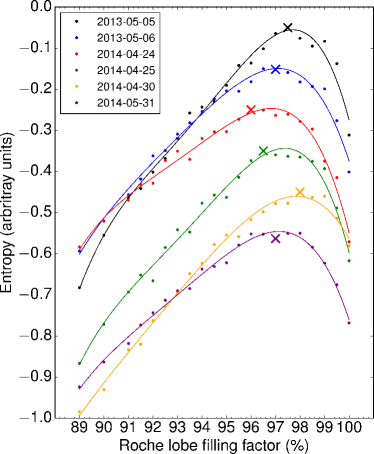
Figure 11: Points show the map entropy obtained in each data set as a function of RLFF, where optimal masses were used for each RLFF. The optimal systemic velocities found in Section 4.2.2 were adopted for the map reconstructions. The points are plotted with a vertical offset of 0.1 between data sets. Crosses mark the maps of maximum entropy, yielding the optimal masses at the optimal RLFF. Fourth-order polynomial fits are shown as a visual aid. The peaks of these fits were not used to determine the optimal RLFF, as the high-order nature of the polynomial meant the fits were often skewed. The mean RLFF across all data is $97\pm 1$ per cent, where the uncertainty represents the spread between maximum and minimum for all measured values.

Readers should note that, unless otherwise stated, the value of the RLFF is given as the ratio of the volume averaged radius of the M star to its Roche lobe radius, as opposed to the linear RLFF which is given by the distance from the centre of mass of the M star to its surface in the direction of the L1 point divided by the distance to the L1 point.

Figure 11 shows the map entropy as a function of RLFF. For a given RLFF, the optimal masses are determined by reconstructing maps for many pairs of component masses. The optimal $M_{1}$ and $M_{2}$ are those that produce the map of maximum entropy (an ‘entropy landscape’, see Figure 8 of Hill et al. 2014). The values of $\gamma$ determined in Section 4.2.2 were adopted for the fits, and reconstructions were performed in steps of 0.5 per cent for the RLFF, and in steps of 0.1$\mathrm{M_{\odot}}$ for the masses. The points follow a roughly parabolic trend with some small ‘jumps’ in entropy that are mainly due to the change in grid geometry, due to varying masses and RLFF, combined with rounding errors in the code. However, all optimum RLFFs determined from each independent data set are in close agreement, ranging between 96–98 per cent, and so we can be confident that the measured RLFF and masses are robust. The amount of scatter in the entropy ‘parabolas’ is consistent with the low SNR of the data being fit – similar scatter was found when performing Roche tomography with relatively low-quality data of the CVs AM Her and QQ Vul (Watson et al., 2003).

There are a number of possible sources of systematic error when fitting data of poor SNR with Roche tomography. In this instance, the dominant source of uncertainty in the system parameters is due to the difficulty in determining the true continuum level of the LSD profiles, as discussed in Section 4.1. If the continuum is too low, the Roche lobe is artificially inflated to fit the line wings, resulting in larger measured masses. Furthermore, if the continuum is set too high, the Roche lobe is artificially under-filled. To determine the impact of choosing an incorrect continuum level, a range of offsets were added to the LSD profiles, and for each offset, the LSD profiles were fit and scaled as described in Section 4.1. The optimal masses found for each offset were then compared and, across all data, the maximum difference between the optimal primary and secondary masses were 3.8 per cent and 7.9 per cent, respectively, and the spread in RLFF was 1 per cent. Hence, while only a visual check was made of the fits to the continuum level of each set of LSD profiles, the optimal masses and RLFF found for each data set agree within these uncertainties.

The mean RLFF is $97\pm 1$ per cent, with the mean of the masses yielding $M_{\mathrm{WD}}=0.76_{-0.01}^{+0.02}$$\mathrm{M_{\odot}}$ and $M_{\mathrm{dM}}=0.358_{-0.018}^{+0.022}$$\mathrm{M_{\odot}}$, respectively, where all uncertainties represent the spread between the maximum and minimum values. Hence, the mean mass-ratio was found to be $q=0.47\pm 0.04$. In Section 5 we will combine the spectroscopic constraints with our light curve data to determine more precise values for these parameters, but quote these Roche tomography values here for completeness. Using the mean system parameters with our model grid, we calculate $v\sin{i}$ to range between a minimum of 117.8$\mathrm{km\,s^{-1}}$ at phase 0 and 0.5, to a maximum of 133.5$\mathrm{km\,s^{-1}}$ at phase 0.25 and 0.75. Our measured masses and RLFF agree well across all data sets, and so for consistency in comparing maps, we adopted the mean values for the final map reconstructions (see Figure 13).

Figure 12: Trailed LSD profiles of QS Vir using phase-binned data from all data sets. A mean of the computed LSD profiles has been subtracted from both the observed and computed LSD profiles. Starspot features in these panels appear dark. The orbital motion has been removed assuming the binary parameters found in Section 4.2.

4.3 Surface maps

The mean system parameters found in Section 4.2 were used to construct Roche tomograms of all data sets. The corresponding trails of LSD profiles are displayed in Figure 9. Evident in both the trails and the maps are numerous spot features, with three large-scale features common to all trails and maps (marked A, B and C in Figures 12 and 13). The technique of Roche tomography is shown to be remarkably robust in the reconstruction of these features – maps reconstructed independently with data taken on sequential nights show very similar features. The morphologies of these three features remain fairly unchanged over the 1 year period of observations, with no apparent movement across the stellar surface, indicating that these are indeed long-lived starspots. Furthermore, smaller-scale structure is apparent in both the data and fits from the 2013 data, however the same level of detail is not as readily reconstructed using other data sets, most likely due to the fewer number of LSD profiles being fit.

There is a distinct lack of a large high-latitude spot. Such a feature is commonly seen on Doppler imaging studies of rapidly rotating single stars (e.g. Donati et al., 1999; Hussain et al., 2007), and in CVs such as BV Cen and AE Aqr (Watson et al., 2007, 2006). Given the presence of such a feature in these other rapidly rotating stars, it is surprising to find that a large high-latitude spot does not exist here. Pertinently, a study by Morin et al. (2008) finds that large-scale, mainly axisymmetric poloidal fields are fairly common in fully convective M dwarfs, observing polar region spots on three out of the six stars in their sample. However, the authors also found that the partly convective star AD Leo hosted a similar magnetic field, but with significantly lower magnetic flux, indicating the generation of large-scale magnetic fields is more efficient in fully convective stars. As the measured mass of the M dwarf in QS Vir suggests it has a partly radiative core, the lower efficiency of magnetic field generation may mean any polar region spots are significantly less obvious.

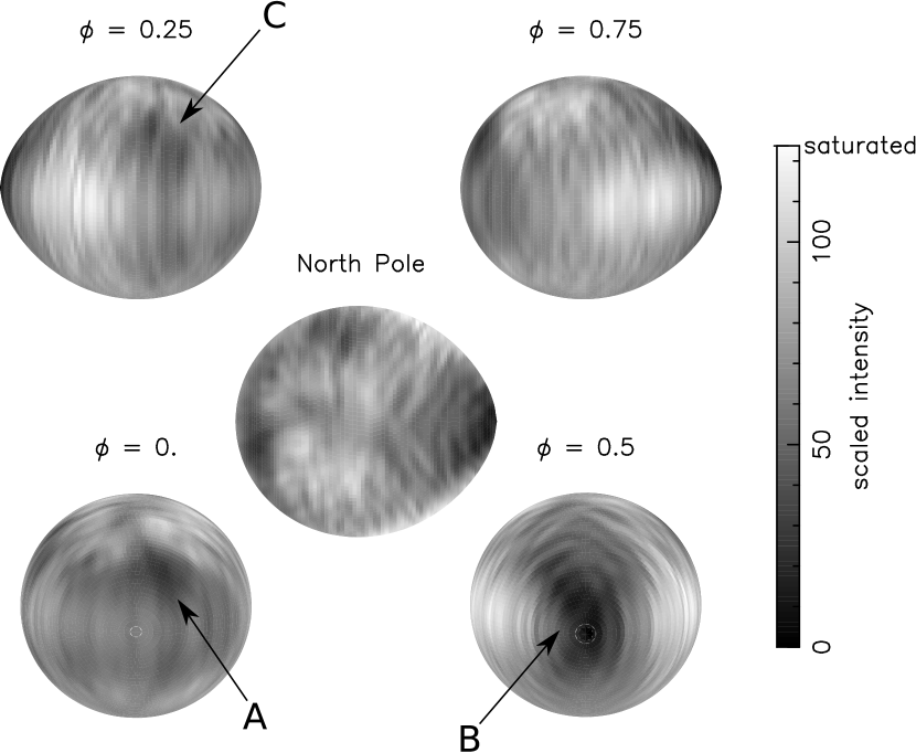
Figure 13: Roche tomogram of QS Vir using phase-binned data from all data sets. Dark grey scales indicate regions of reduced absorption line strength that is due to either the presence of starspots or the impact of irradiation. The contrast in these Roche tomograms has been enhanced such that the darkest and lightest grey-scales correspond to the lowest and highest intensities in the reconstructed map. The orbital phase is indicated above each panel, and Roche tomograms are shown without limb darkening for clarity.

Alternatively, the lack of a large high-latitude feature may simply be due observational effects – given the inclination of $i=77.8\degr$ in QS Vir, high latitudes appear severely foreshortened, and are heavily limb-darkened. These effects, combined with the poor SNR of the data, may mean high-latitude features are simply lost in the noise. This was assumed to be the case by Barnes & Collier Cameron (2001) who found a similar lack of polar spot features in their study of HK Aqr ($i=70-90^{\circ}$), with simulations showing that reconstructions of high-latitude features strongly depend on the SNR of the data.

Other prominent features on the maps are the dark regions around the L₁ point, marked ‘B’ in Figures 12 and 13. In previous maps of CVs (e.g. Watson et al. 2003) features on this part of the star were attributed to irradiation effects from the white dwarf, where ionisation of the photosphere causes a decrease in photometric flux. However, the features reconstructed here are patchy in morphology, rather than smoothly varying, which suggests that irradiation is not the main contributing factor of the features in this region. This was tested by simulating a realistic irradiation pattern, and fitting the data using the same phases as that of the phase-binned LSD profiles shown in Figure 12. The reconstructed irradiation pattern was found to be smoothly varying, and was essentially uniform around the front of the star. Likewise, the effect of gravity darkening on map reconstruction was simulated using a gravity darkening coefficient of $\beta\sim 0.1$, as found by Djurašević et al. (2003, 2006) for late-type M stars. The simulated map showed the effects of gravity darkening to be smoothly varying, with minimal contribution to the mapped features. In addition, the dominant features in the line profiles between phases 0.4–0.6 (as noted in Section 4.1) were thought to originate off the stellar surface, and so these phases were excluded from the fit. Hence it is unlikely that circumstellar material is the source of these patches around the L₁ point.

We conclude that there is significant spot coverage on the inner hemisphere (white dwarf facing side of the M star) observed on all maps. This spot distribution – where there is a higher density of spots on the hemisphere facing the companion star – is similar to that observed in many other systems, such as the pre-CV V471 Tau (Hussain et al., 2006), the eclipsing binary ER Vul (Xiang et al., 2015), and the close binary $\sigma^{2}\text{CrB}$ (Strassmeier & Rice, 2003). Furthermore, Kriskovics et al. (2013) suggested that the hot-spots mapped on the companion-facing hemisphere in V824 Ara may indicate the strong interaction between the magnetic fields of the component stars, as is commonly observed in close RS CVn-type binaries. This phenomenon was discussed in Hill et al. (2014), where spot ‘chains’ from the pole to L₁ point (on multiple CVs) suggested a mechanism that forces magnetic flux tubes to preferentially emerge at these locations. Indeed, Holzwarth & Schüssler (2003) propose that tidal forces may cause spots to form at preferred longitudes, and Moss et al. (2002) suggest that this phenomena may also be due to the tidal enhancement of the dynamo action itself.

Other features of interest include a prominent starspot labelled ‘A’ in Figure 13. It stretches $\sim 5$–25^∘ in longitude, and $\sim 15$–35^∘ in latitude (where the back of the star is at $0^{\circ}$ longitude, with increasing longitude in the direction of the leading hemisphere). Finally, label ‘C’ in Figure 13 points to a group of spots covering 275–300^∘ longitude and spanning 20–55^∘ latitude. Given that the phase-binned data has a longitudinal resolution of $\sim 6^{\circ}$, we can reliably separate the larger spots in this group – one spot extends 275–285^∘ longitudinally and 35–55^∘ in latitude, and another spans 293–300^∘ in longitude and 15–30^∘ latitudinally. As both ‘A’ and ‘C’ can be seen in all data trails taken over a $\sim 1$ yr period, they are most likely groups of long-lived starspots.

The prominent spotted regions labelled ‘A’ and ‘B’ (located at phases $\phi\sim 0.05$ and $\phi\sim 0.5$, respectively) are similar to those found by Ribeiro et al. (2010) in their maps of QS Vir made using photometry taken in 1993 and 2002. The authors find two cool regions at $\phi\sim 0.4$ and $\phi\sim 0.9$ that show little shift in longitude between 1993 and 2002. The authors’ photometric data does not allow for a tight constraint on latitude, however, if these spotted regions are the same as those imaged here (namely features ‘A’ and ‘B’), they may be very long lived active regions that have remained at the same longitudes for over 20 years.

4.3.1 Spot coverage as a function of longitude and latitude

To make a more quantitive estimate of spot parameters on QS Vir, we have examined the pixel intensity distribution in the Roche tomogram. By visual inspection, all reconstructed maps appeared to have a very similar distribution of spots, with small-scale variation due to differences in SNR and number of spectra between data sets. For an improved estimate of spot coverage, we combined all data sets by phase-binning the LSD profiles over 60 evenly-spaced phase bins (each containing $\sim 7$ LSD profiles). We only present analysis of the map that was reconstructed using this binned data (see Figure 13).

The high inclination of the system causes a ‘mirroring’ effect, as described in section 3.11 of Watson & Dhillon (2001). As radial velocities cannot constrain whether a feature is located in the Northern or Southern hemisphere, features are mirrored about the equator. This means features become less apparent due to the fact that they are first latitudinally smeared, and then mirrored, causing the streaks seen in the maps presented here. To mitigate this effect, we discarded all pixels in the Southern hemisphere for the remainder of this analysis.

Each pixel in our Roche tomograms was given a spot filling-factor between 0 (immaculate) to 1 (totally spotted). The value for any given pixel depended on its intensity, and was scaled linearly between our predefined immaculate and spotted photosphere intensities. It is unlikely that the highest intensities represent the immaculate photosphere, as the growth of bright pixels in maps that are not ‘threshholded’ is a known artefact of Doppler imaging techniques (e.g. Hatzes & Vogt, 1992). Instead, we have defined an intensity of 92 and above to represent the immaculate photosphere. Furthermore, we have defined a 100 per cent spotted pixel by taking the minimum pixel intensity in the group of spots marked ‘B’ in Figure 13, avoiding the very front pixels on the model star as these may be additionally affected by gravity darkening or irradiation.

Based on our classification of a spot, we estimate that 35 per cent of the northern hemisphere of QS Vir is spotted. This is likely to be a lower limit due to the presence of unresolved spots – O’Neal et al. (1998) estimated up to 50 per cent fractional spot coverage in TiO studies of rapidly-rotating G and K type stars, and Senavci et al. (2015) find a factor $\sim 10$ difference between spot filling factors when comparing TiO analysis to Doppler imaging. Furthermore, Hessman et al. (2000) predict a mean spot coverage of $\sim 50$ per cent on the CV, AM Her, using long-term light curve analysis.

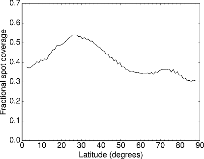
Figure 14: Fractional spot coverage as a function of latitude, normalised by the surface area of that latitude, as calculated for the reconstructed map using phase-binned data. The geometry the grid in our Roche tomogram does not allow for strips of constant latitude, and so we are required to interpolate between grid elements. We have done this by taking a moving-mean with a $5^{\circ}$ window in steps of $1^{\circ}$.

When plotted as a function of latitude (see Figure 14) we see a clear increase in fractional spot coverage at low to mid latitudes (10–50^∘) of around 0.2, as compared to the spot coverage at higher latitudes (50–90^∘). This large spread in latitude may be indicative of a distributed dynamo, with many unresolved small-scale features spread across the stellar surface. A more likely explanation, however, is that the spread is due to features becoming smeared in latitude due to both poor SNR, and from limitations in the technique (as discussed above). Also apparent is a small increase in spot coverage at high latitudes (centred $\sim 74^{\circ}$). As discussed above, the spot contrast at higher latitudes is diminished in this system due to is high inclination, and so the measured spot coverage is likely underestimated at these latitudes. Similar distributions of spots were found on the M dwarfs HK Aqr and RE 1816+541 by Barnes & Collier Cameron (2001), with the majority of features equally distributed over 20–80^∘ latitude.

When plotted as a function of longitude in Figure 15, we find a large increase in fractional spot coverage around $15^{\circ},180^{\circ}$, and $285^{\circ}$ longitude, corresponding to the features marked A, B and C, respectively, as shown in Figure 13. As previously discussed, the large increase around $180^{\circ}$ is similar to that found on CVs (e.g. AE Aqr, Hill et al. 2014) and on pre-CVs (e.g. V471 Tau, Hussain et al. 2006).

4.3.2 Magnetic activity and star spot lifetime

The features marked A, B and C in Figures 12 and 13 are clearly observed in all data sets from May 2013 to April 2014, and appear to remain in fixed positions over both short and long timespans. This suggests a very low level of surface shear, with no perceivable shift over the $\sim 1$ yr between first and last observations. As the M star in QS Vir is very close to becoming fully convective, the lack of any detectable differential rotation concurs with the conclusions of Barnes et al. (2005), who found that differential rotation appears to vanish with increasing convection depth. This trend was also found in studies of rapidly-rotating M dwarfs by Morin et al. (2008), where several stars in their sample exhibited fairly similar magnetic topologies over the $\sim 1$ yr period between observations. In other work, Morin et al. (2010) found both GJ 51 and WX UMa to exhibit strong, large-scale axisymmetric-poloidal and nearly dipolar fields, with very little temporal variations over the course of several years.

We see no evidence of a magnetic activity cycle in our observations. O’Donoghue et al. (2003) suggested that the $\pm 12$ s spread on ephemerides over their 10 years of eclipse timings may be due to such a cycle. This appears unlikely, since their Figure 3 (b) shows a $\sim 0.12$ per cent period change in $\sim 600$ d – One would expect spot migration to occur over the course of a magnetic activity cycle, as seen on the Sun, and as we find spot features are stable over a $\sim 1$ yr period, such a cycle cannot be responsible for this rapid change in period.

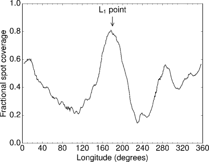
Figure 15: Fractional spot coverage as a function of longitude, as calculated for the reconstructed map using phase-binned data. Points are calculated by taking a moving-mean with a $6^{\circ}$ window (the longitudinal resolution of the map), in steps of $1^{\circ}$.

These features may well be related to the large prominences that pass in front of both stars. Since the prominences appear to be stable on a timescale of years, they must still be anchored to the surface of the M star by its magnetic field. Starspots are likely to form near these anchor regions, as is seen in solar coronal loops and prominences.

5 Modelling the eclipse light curve

Eclipsing PCEBs have been used to measure precise masses and radii of both the white dwarf and main-sequence components in a number of systems (e.g. Parsons et al., 2010a, 2012a, 2012b) offering some of the most precise and model-independent measurements to date for either type of star. The small size of the white dwarf leads to very sharp eclipse features, with typical ingress and egress times of around a minute or less meaning that high-speed photometry is required to properly resolve the eclipse features. With typical exposure times of $<3$ sec, our ULTRACAM data fully resolve the eclipse of the white dwarf and thus can be used to place stringent constraints on the physical parameters of both stars.

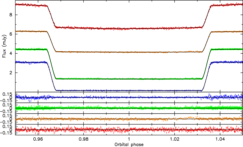
Figure 16: Flux calibrated ULTRACAM $u^{\prime}g^{\prime}r^{\prime}$ and $i^{\prime}$ band light curves of the eclipse of the white dwarf in QS Vir with model fits overplotted (black lines). We have offset the $i^{\prime}$ band light curve by -13mJy to show more detail. The bottom four panels show the residuals of the fit in the $u^{\prime}$ band (top panel, blue points), $g^{\prime}$ band (second panel, green points), $r^{\prime}$ band (third panel, orange points) and the $i^{\prime}$ band (bottom panel, red points).

We model the light curve data using a code written for the general case of binaries containing white dwarfs (see Copperwheat et al. 2010 for a detailed description). The program subdivides each star into small elements with a geometry fixed by its radius as measured along the direction of centres towards the other star with allowances for Roche geometry distortion. We fitted the ULTRACAM $u^{\prime}g^{\prime}r^{\prime}$ and $i^{\prime}$ band light curves around the eclipse of the white dwarf. We exclude data taken at other orbital phases since the effects of starspots on the surface of the main-sequence star strongly influences the constraints that these data provide. However, the effects of starspots on the white dwarf eclipse itself are minor, since it is such a rapid process. Nevertheless, starspots often lead to linear slopes across the eclipse, that vary over the timescale of our ULTRACAM observations. Therefore, each eclipse observation was initially fitted with a basic model using the parameters from Parsons et al. (2010b) and including a linear slope. This slope was then removed from each light curve individually before combining them. Additionally, we shifted each eclipse in phase to remove the effects of the deviations from linearity in the eclipse arrival times.

The basic geometric parameters required to define the model are the mass ratio, $q=M_{\mathrm{sec}}/M_{\mathrm{WD}}$, the inclination, $i$, the scaled radii of both stars, $R_{\mathrm{WD}}/a$ and $R_{\mathrm{sec}}/a$ and the two temperatures, $T_{\mathrm{eff,WD}}$ and $T_{\mathrm{eff,sec}}$. In addition to these, the model also requires the time of mid eclipse, $T_{0}$, the period, $P$ and the limb darkening parameters for both stars.

Since we used phase-folded data we kept the period fixed as 1, but allowed $T_{0}$ to vary. The temperature of the white dwarf was fixed at $T_{\mathrm{eff}}=$14,220 K. We use the same setup for limb darkening as detailed in Equation 3 for both stars. For the M star, we use the limb darkening coefficients for a $T_{\mathrm{eff}}=$3,100 K, $\log{g}=5$ main sequence star in the appropriate filter (Claret, 2000). We use the coefficients for a $T_{\mathrm{eff}}=$14,000 K, $\log{g}=8.25$ white dwarf from Gianninas et al. (2013). All these limb darkening coefficients were kept fixed during the fitting process.

The profile of the eclipse of the white dwarf does not contain enough information to simultaneously constrain the inclination and the scaled radii of both stars, only how they relate to each other. Therefore, an additional constraint is required to break this degeneracy. Ideally we would use the secondary eclipse (the transit of the white dwarf in front of the M star, see Parsons et al. 2010a for example), but for QS Vir this is too shallow to detect in our ULTRACAM data. An alternative method would be to use the amplitude of the ellipsoidal modulation, which is related to the mass ratio (which we have already spectroscopically constrained) and the scaled radius of the M star (e.g. Parsons et al., 2012b). However, the effects of starspots make this approach unreliable, even with the Roche tomography results. Moreover, this limits our fits to the longer wavelength bands where the M star dominates and hence where the white dwarf eclipse is shallower and offers poorer constraints on its size. Therefore, this approach was not taken, although we did check that our final model results predicted an ellipsoidal modulation amplitude consistent with the ULTRACAM data. Another method used to break the degeneracy between the inclination and scaled radii, and that we use here, is to use our measurement of the rotational broadening of the M star ($V_{\mathrm{rot}}\sin{i}$). For a synchronously rotating star this is given by

$$V_{\mathrm{rot}}\sin{i}=K_{\mathrm{sec}}(1+q)\frac{R_{\mathrm{sec}}}{a},$$ (4)

where the radial velocity semi-amplitude of the M star ($K_{\mathrm{sec}}$) and the mass ratio ($q$) have both been spectroscopically constrained. Hence, combining this with the fit to the white dwarf eclipse allows us to determine the inclination, radii of both stars and, via Kepler’s laws, the orbital separation and masses of both stars. However, as previously noted in section 4.2.3, the measured rotational broadening varies as a function of orbital phase, as the M star is not spherical and hence presents a different radius at different orbital phases. Therefore, when fitting the eclipse light curve we calculated the rotational broadening of the M star at the quadrature phases (when it is at its maximum) and compared this to the maximum value determined from our Roche tomography analysis.

We used the Markov Chain Monte Carlo (MCMC) method to determine the distributions of our model parameters (Press et al., 2007). The MCMC method involves making random jumps in the model parameters, with new models being accepted or rejected according to their probability computed as a Bayesian posterior probability. In this instance this probability is driven by a combination of the $\chi^{2}$ and the prior probability from our constraints from the spectroscopy and Roche tomography. For each band an initial MCMC chain was used to determine the approximate best parameter values and covariances. These were then used as the starting values for longer chains which were used to determine the final model values and their uncertainties. Several chains were run simultaneously to ensure that they converged on the same values.

This approach results in very few systematic uncertainties in the derived parameters, since the vast majority of them are directly determined by the data itself. The temperatures of the two stars are effectively scale factors and so have no effect. The shape of the eclipse of the white dwarf is not altered by the adopted limb darkening coefficients for the M star, these are mostly important for the transit of the white dwarf across the face of the M dwarf as well as any ellipsoidal modulation, neither of which we consider in our fit. However, the choice of limb darkening coefficients for the white dwarf does have some effect on the final parameters, specifically the final radius measurement for the white dwarf (and to a lesser extent the M dwarf). To determine how large this effect is we re-fitted the eclipse light curves using limb darkening coefficients for a white dwarf with $T_{\mathrm{eff}}=13,500$ K and $T_{\mathrm{eff}}=14,500$ K and $\log{g}=8.00$ and $\log{g}=8.50$, taken from Gianninas et al. (2013), these bracket the coefficients that we used in our final fit. We found that the differences in the final parameters were smaller than their statistical uncertainties, implying that the white dwarf’s limb darkening coefficients have a very minor effect on the fit.

The only other source of systematic uncertainty in the light curve fit arises from the Roche tomography analysis. As previously mentioned, we used the rotational broadening and M dwarf radial velocity semi-amplitude measurements from the Roche tomography analysis to help break the degeneracies in the light curve fit. However, as Figures 10 and 11 show, the values vary slightly from night to night. This was taken into account by increasing the uncertainties on these two values to cover the spread of values seen on different nights. Indeed, this is the largest source of uncertainty in the fit and limits how precisely we could measure the stellar masses.

Table 2: Stellar and binary parameters of QS Vir. The orbital period and T0 values were taken from Parsons et al. (2010b), the distance and white dwarf temperature values were taken from O’Donoghue et al. (2003).

Parameter	Value
RA	13:49:51.95
Dec	-13:13:37.5
Orbital period	0.150 757 463(4)
T0 (BMJD(TDB))	48689.14228(16)
Distance	$48\pm 5$pc
$K_{\mathrm{WD}}$	$139.0\pm 1.0$$\mathrm{km\,s^{-1}}$
$\gamma_{\mathrm{WD}}$	$43.2\pm 0.8$$\mathrm{km\,s^{-1}}$
$K_{\mathrm{sec}}$	$275.8\pm 2.0$$\mathrm{km\,s^{-1}}$
$\gamma_{\mathrm{sec}}$	$-4.4_{-0.9}^{+0.5}$$\mathrm{km\,s^{-1}}$
Mass ratio	$0.489\pm 0.005$
Orbital separation	$1.253\pm 0.007$$\mathrm{R_{\odot}}$
Orbital inclination	$77.7^{\circ}\pm 0.5^{\circ}$
White dwarf mass	$0.782\pm 0.013$$\mathrm{M_{\odot}}$
White dwarf radius	$0.01068\pm 0.00007$$\mathrm{R_{\odot}}$
White dwarf $\log{g}$	$8.274\pm 0.009$
White dwarf effective temperature	14,220$\pm 350$K
M star mass	$0.382\pm 0.006$$\mathrm{M_{\odot}}$
M star radius sub-stellar	$0.466\pm 0.003$$\mathrm{R_{\odot}}$
M star radius polar	$0.365\pm 0.003$$\mathrm{R_{\odot}}$
M star radius backside	$0.416\pm 0.003$$\mathrm{R_{\odot}}$
M star radius volume-averaged	$0.381\pm 0.003$$\mathrm{R_{\odot}}$

The best fit models to the white dwarf eclipse in the $u^{\prime}g^{\prime}r^{\prime}$ and $i^{\prime}$ bands are shown in Figure 16, along with their residuals. The results from all four bands were consistent and the final stellar and binary parameters are detailed in Table 2. The results are consistent with those of O’Donoghue et al. (2003), but a factor of 4 more precise in mass and almost 10 in radius. In fact, the radius measurement of the white dwarf in QS Vir is the most precise, direct measurement of a white dwarf radius ever. It is remarkable that we have measured the size of an object at nearly 50pc away to within 50km, and highlights the potential for these kinds of systems to strongly test theoretical mass-radius relationships. The measured masses of the two stars are also consistent with the results from Roche tomography ($M_{\mathrm{WD}}=0.76\pm 0.01$$\mathrm{M_{\odot}}$, $M_{\mathrm{dM}}=0.36\pm 0.02$$\mathrm{M_{\odot}}$).

An additional constraint on the stellar parameters comes from the gravitational redshift of the white dwarf. For the measured parameters listed in Table 2 we would expect to measure a redshift for the white dwarf of $45.8\pm 0.6$$\mathrm{km\,s^{-1}}$ (taking into account the redshift of the M star, the difference in transverse Doppler shifts and the potential at the M star owing to the white dwarf). Taking the difference between the systemic velocities of the two stars from our UVES data gives a measured gravitational redshift of $47.6\pm 1.2$$\mathrm{km\,s^{-1}}$, which is fully consistent with our results.

6 Discussion

6.1 The mass-radius relationship for white dwarfs

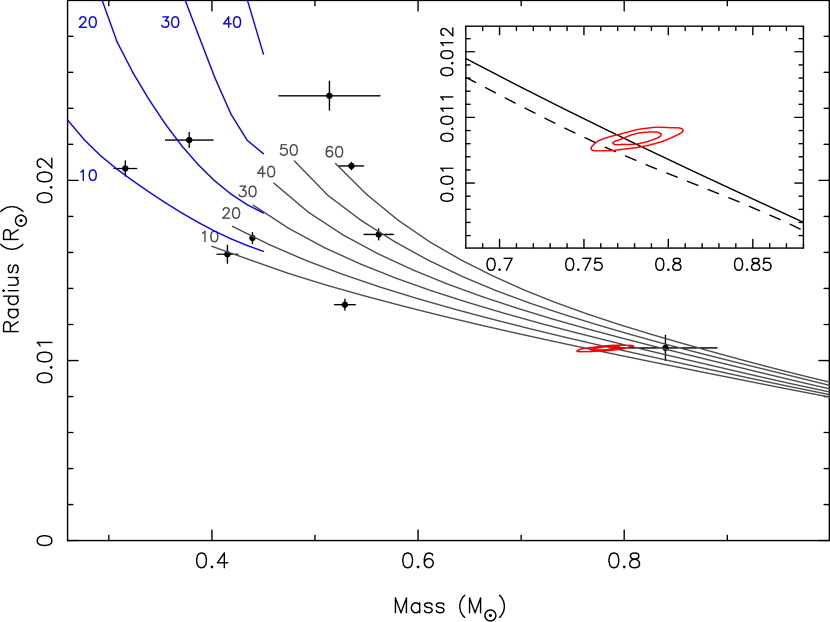
Figure 17: White dwarf mass-radius relation. We show the measured values for the white dwarf in QS Vir as red contours (68 and 95 percentile regions). Also shown as black points are other direct mass-radius measurements from eclipsing PCEB systems (O’Brien et al., 2001; Pyrzas et al., 2012; Parsons et al., 2010a, 2012a, 2012b, 2012c; Bours et al., 2014, 2015). Theoretical mass-radius relationships for carbon-oxygen core white dwarfs are shown in grey (Benvenuto & Althaus, 1999) and helium core white dwarfs in blue (Panei et al., 2007), labelled by temperature in thousands of Kelvin and for hydrogen envelope thicknesses of M_H/M${}_{\mathrm{WD}}=10^{-4}$. Inset we show a zoom of the measured QS Vir parameters with a theoretical mass-radius relationship for a 14,200K white dwarf with a thick hydrogen envelope (M_H/M${}_{\mathrm{WD}}=10^{-4}$, solid line) and a thin envelope (M_H/M${}_{\mathrm{WD}}=10^{-6}$, dashed line), showing that the measured parameters are in excellent agreement with the theoretical models for a white dwarf with a thick hydrogen envelope.

Figure 17 shows the mass-radius plot for white dwarfs and highlights the location of the white dwarf in QS Vir. We also plot the model-independent mass-radius measurements of several other white dwarfs, all members of close, eclipsing binaries. Inset we show a zoom in on the white dwarf in QS Vir compared to theoretical models. The measured values show excellent agreement with a carbon-oxygen core white dwarf model of the same temperature and with a thick hydrogen envelope (M_H/M${}_{\mathrm{WD}}=10^{-4}$), although the uncertainty in the measurements mean that thinner hydrogen layers cannot be ruled out. This is consistent with the results from other white dwarfs in PCEBs, such as NN Ser and GK Vir, which both possesses hydrogen envelope masses of M_H/M${}_{\mathrm{WD}}=10^{-4}$ (Parsons et al., 2010a, 2012a), although several other eclipsing white dwarfs have thinner hydrogen envelopes e.g. SDSS J0138-0016 (M_H/M${}_{\mathrm{WD}}=10^{-5}$, Parsons et al. 2012b) and SDSS J1212-0123 (M_H/M${}_{\mathrm{WD}}=10^{-6}$, Parsons et al. 2012a). Both white dwarf components of the eclipsing binary CSS 41177 appear to have thin hydrogen layers as well (M_H/M${}_{\mathrm{WD}}<10^{-4}$, Bours et al. 2014). The only other reliable white dwarf hydrogen envelope mass measurement in a PCEB system is for the pulsating white dwarf in SDSS J1136+0409, which was found to have an envelope mass of M_H/M${}_{\mathrm{WD}}=10^{-4.9}$ (Hermes et al., 2015), implying that there could be a substantial spread in the hydrogen envelope masses of white dwarfs in PCEBs, possibly as a result of the common envelope phase itself.

The temperature and surface gravity of the white dwarf in QS Vir place it close to the blue edge of the DA white dwarf instability strip. However, our results are precise enough to firmly place it just outside the strip, which is consistent with the null detection of pulsations in our extensive high-precision photometry.

6.2 The mass-radius relationship for low-mass stars

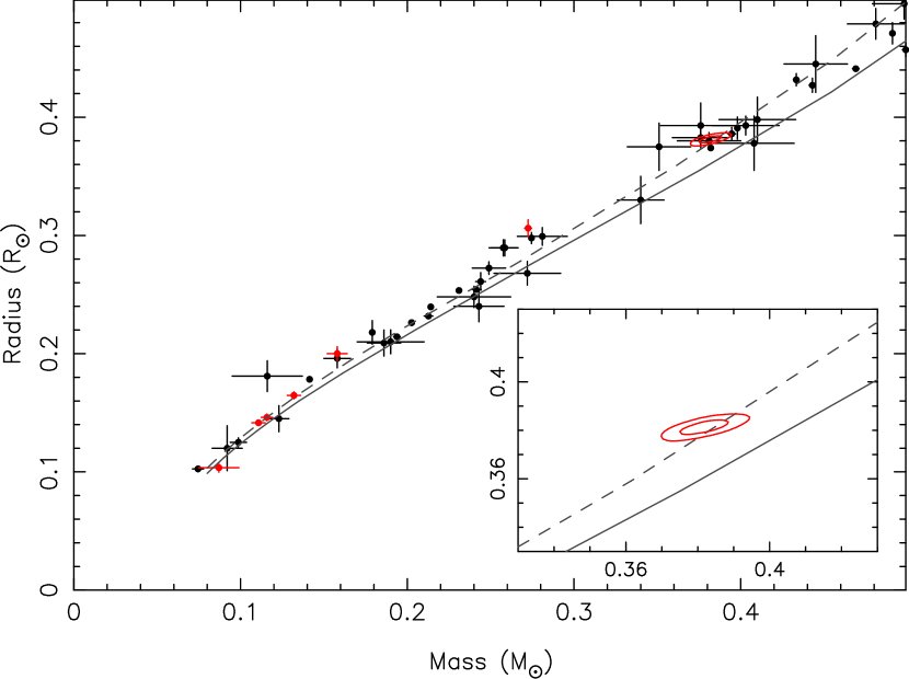
Figure 18: Low-mass star mass-radius relation. We show the measured values for the main-sequence star in QS Vir (volume-averaged radius) as red contours (68 and 95 percentile regions). Also shown as red points are other direct mass-radius measurements from eclipsing PCEB systems (Pyrzas et al., 2012; Parsons et al., 2010a, 2012a, 2012b, 2012c). The black points are other direct mass-radius measurements taken from Gómez Maqueo Chew et al. (2014). The solid grey line is the theoretical mass-radius relation for a 1 Gyr main-sequence star (Baraffe et al., 1998), while the grey dashed line is for an active star of the same age (Morales et al., 2010). Inset we show a zoom of the measured QS Vir parameters showing that the radius is consistent with a theoretical active star of the same mass.

In Figure 18 we show the mass-radius plot for low-mass ($<$0.5$\mathrm{M_{\odot}}$) stars along with a number of directly measured objects. The location of the M star in QS Vir is indicated by the contours, where we have used the volume-averaged radius. Its mass and radius measurements are consistent with the evolutionary models of Morales et al. (2010) for a 1 Gyr magnetically active star. Also highlighted in red are several other low-mass star mass-radius measurements from PCEB systems. The M star in QS Vir is the first low-mass star in a PCEB that is not fully convective (M${}_{\mathrm{dM}}>$0.35$\mathrm{M_{\odot}}$) to have high-precision, model-independent mass and radius measurements. While the majority of these measurements are consistent with theoretical models, two systems (SDSS J1212-0123, Parsons et al. 2012a and SDSS J1210+3347 Pyrzas et al. 2012) have measured radii almost 10 per cent over-inflated compared to these same models. Any possible explanation for why some of these low-mass stars are over-inflated, while others aren’t will require more high-precision mass-radius measurements from PCEBs and more theoretical modelling of low-mass stars.

6.3 The current evolutionary state of QS Vir

The strong surface gravity of the white dwarf causes metals to sink out of the photosphere on a short timescale. Therefore, the detection of the Mg ii 4481Å absorption line implies that the white dwarf must be currently accreting some material originating from the M star. Interestingly, the strength of this absorption is variable as shown in Figure 19. It was slightly stronger in 2014 compared to 2013. This supports the idea that the accretion rate of material onto the white dwarf is variable on year timescales and is unlikely to originate solely from the wind of the M star, but is likely driven by flare and coronal mass ejections (CME) events.

Matranga et al. (2012) detected clear X-ray eclipses, revealing that the white dwarf dominated the X-ray flux rather than the M star, supporting the idea of ongoing accretion. They determined an accretion rate of $\dot{M}=1.7\times 10^{-13}\mathrm{M}_{\odot}\mathrm{yr}^{-1}$, which would be one of the lowest accretion rates for a non-magnetic CV system if this were the case, but would be particularly large for a detached system. The authors speculate that a stellar wind could be the source of the observed mass transfer, invoking a magnetic ‘syphon’ model, as found by Cohen et al. (2012). Matranga et al. (2012) speculated that to maintain a more constant mass supply, the wind could be supplemented by upward chromospheric flows, analogous to spicules and mottles on the Sun.

Figure 19: Equivalent width of the Mg ii 4481Å absorption line from the white dwarf as a function of time. The strength of the line appears to be variable on year timescales, implying that the accretion rate of wind material on to the white dwarf is not constant.

Conversely, Drake et al. (2014) used the HST spectra taken by O’Donoghue et al. (2003) in 1999 to calculate an accretion rate of $10^{-16}\mathrm{M}_{\odot}\mathrm{yr}^{-1}$, around one thousand times lower than that found 6.5 years later by Matranga et al. (2012). This accretion rate is more consistent with a wind accretion, and is an order of magnitude lower than the wind accretion rate inferred for similar pre-CVs (Debes, 2006; Tappert et al., 2011; Parsons et al., 2012a). This supports the idea that CME and prominence activity may provide a stochastic source of accretion material.

In Parsons et al. (2011) we used the Mg ii 4481Å absorption line to rule out the $V_{\mathrm{rot}}\sin{i}=400$$\mathrm{km\,s^{-1}}$ rapid rotation of the white dwarf determined by O’Donoghue et al. (2003). The long exposure time of that data (1800 s) meant that the line suffered from substantial smearing and therefore it was consistent with having no measurable broadening and we concluded that the white dwarf was not rapidly rotating. Our new data have much shorter exposure times (180 s) and can place better constraints on its rotational velocity. In Figure 20 we show the Mg ii 4481Å absorption line made by combining all the data, overplotted with the best fit TLUSTY model (Hubeny & Lanz, 1995) with $V_{\mathrm{rot}}\sin{i}=69$$\mathrm{km\,s^{-1}}$. The white dwarf moves by a maximum of $\sim$15$\mathrm{km\,s^{-1}}$ during each exposure, meaning that there is clearly some additional broadening of the line. If this is due to the rotation of the white dwarf then it implies a rotational period of only 700 seconds, extremely fast for a detached system and implies that there may well have been a previous stage of high mass-transfer. To spin up the white dwarf this much would require an average accretion rate of $\sim$$10^{-11}\mathrm{M}_{\odot}\mathrm{yr}^{-1}$ over the entire cooling age of the white dwarf, meaning that QS Vir would almost certainly have to have been a CV in the past. Alternatively, the white dwarf may posses a weak magnetic field. A field strength of $\sim$$10^{5}$G is sufficient to Zeeman split the Mg ii line by 69$\mathrm{km\,s^{-1}}$, mimicking a broadening of the line. This could also help explain the stability of the prominence features, as the interaction of the fields of the two stars may create stable regions.

There are several pieces of evidence that could suggest that QS Vir is a currently detached CV (either hibernating or genuinely detached, similar to a CV crossing the gap). The fact that the binary is very close to Roche-lobe filling, the white dwarf is relatively massive (0.782$\mathrm{M_{\odot}}$, typical for white dwarfs in CVs but relatively rare among PCEBs and pre-CVs Zorotovic et al. 2011) and could be rapidly rotating, may indicate a previous episode of high mass transfer. However, our results argue against this interpretation. The RLFF of 96 per cent (97 per cent from the Roche tomography analysis), means that the M star is still within its Roche lobe, and the fact that its mass and radius are consistent with evolutionary models implies that it is not inflated. In CVs above the orbital period gap the donor stars are oversized by roughly 30 per cent (Knigge et al., 2011) and would take at least $10^{7}$ yr (the thermal timescale of the M star) to relax back to their equilibrium radius once becoming detached (i.e. if QS Vir is a detached CV, then it must have been so for at least $10^{7}$ yr). In this time the period has decreased by $\sim$15 minutes (assuming classical magnetic braking, Rappaport et al. 1983). Hence, if the system is in a hibernating state, then the nova explosion that caused the system to detach would have had to increase the period by $\sim$15 minutes, an unrealistic prospect. Its current period of 3.6 h is also well above the standard period gap. Therefore, we conclude that the system is more likely to be a pre-CV just about to fill its Roche-lobe, and the white dwarf is weakly magnetic, mimicking the effects of rapid rotation. However, confirmation of this will require spectropolarimetry around the Mg ii 4481Å line.

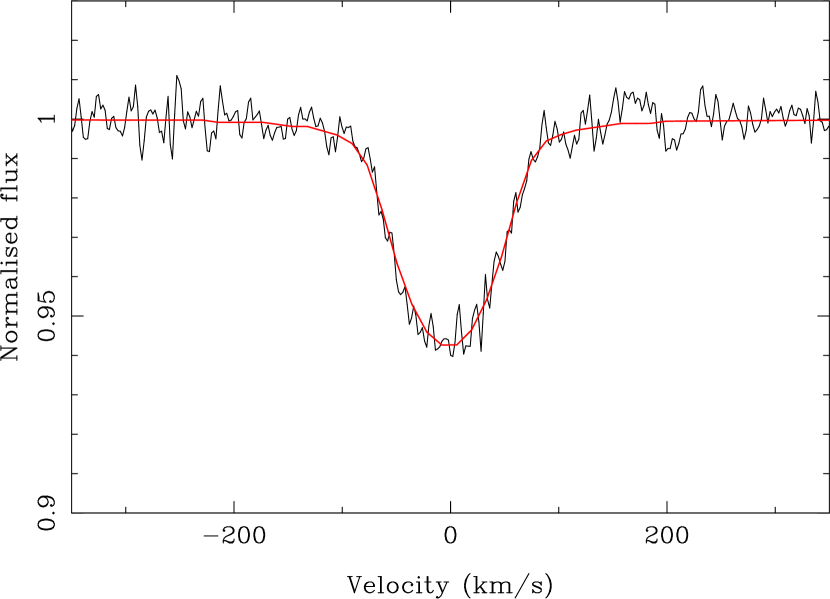
Figure 20: The Mg ii 4481Å absorption line from the white dwarf made by combining all observations. Overplotted in red is a model with $V_{\mathrm{rot}}\sin{i}=69$$\mathrm{km\,s^{-1}}$.

Assuming classical magnetic braking and following the procedure outlined in Schreiber & Gänsicke (2003), we find that QS Vir will fill its Roche lobe at a period of 3.363 hours, in 1.2 Myr. However, the strength of magnetic braking is highly uncertain. For example, replacing the formula given by Rappaport with the normalised prescription used by Davis et al. (2008) results in a significantly longer time until it fills its Roche lobe, i.e. 7.2 Myr. Given that the current cooling age of the white dwarf is 350 Myr the probability of finding a system as close to Roche-lobe filling as QS Vir is approximately half a per cent, which is not implausible given that we now have more than 100 PCEBs with measured periods.

7 Conclusions

We have combined high-resolution phase-resolved UVES spectroscopy and high-speed ULTRACAM photometry of the eclipsing PCEB QS Vir to precisely determine the binary and stellar parameters. We find that both the white dwarf and its low-mass M star companion have radii fully consistent with evolutionary models. The spectroscopy revealed large prominence structures originating from the M star passing in front of both stars. Despite being located in unstable locations within the binary, these prominences appear to be long-lived, lasting more than a year. Using Roche tomography we determined that the M star is covered with a large number of starspots, preferentially located on its inner hemisphere, facing the white dwarf. They too appear to be long-lived and may well be related to the prominences (e.g. located close to where the prominences are anchored to the M star’s surface).

The M star in QS Vir fills 96 per cent of its Roche lobe and the system appears to be a pre-cataclysmic binary, yet to have initiated mass transfer via the inner Lagrange point, rather than a hibernating system. However, the white dwarf may be rapidly rotating, or weakly magnetic, meaning that its past evolution is still uncertain. It will become a cataclysmic variable system in 1.2 Myr with a period above the period gap.

References

- Abazajian et al. (2009) Abazajian, K. N., et al., 2009, ApJS, 182, 543
- Adelman-McCarthy et al. (2008) Adelman-McCarthy, J. K., et al., 2008, ApJS, 175, 297
- Almeida & Jablonski (2011) Almeida, L. A., Jablonski, F., 2011, in Sozzetti, A., Lattanzi, M. G., Boss, A. P., eds., IAU Symposium, vol. 276 of IAU Symposium, p. 495
- Baraffe et al. (1998) Baraffe, I., Chabrier, G., Allard, F., Hauschildt, P. H., 1998, A&A, 337, 403
- Barnes & Collier Cameron (2001) Barnes, J. R., Collier Cameron, A., 2001, MNRAS, 326, 950
- Barnes et al. (2004) Barnes, J. R., Lister, T. A., Hilditch, R. W., Collier Cameron, A., 2004, MNRAS, 348, 1321
- Barnes et al. (2005) Barnes, J. R., Collier Cameron, A., Donati, J.-F., James, D. J., Marsden, S. C., Petit, P., 2005, MNRAS, 357, L1
- Benvenuto & Althaus (1999) Benvenuto, O. G., Althaus, L. G., 1999, MNRAS, 303, 30
- Bours et al. (2015) Bours, M. C. P., Marsh, T. R., Gänsicke, B. T., Parsons, S. G., 2015, MNRAS, 448, 601
- Bours et al. (2014) Bours, M. C. P., et al., 2014, MNRAS, 438, 3399
- Claret (2000) Claret, A., 2000, VizieR Online Data Catalog, 336, 31081
- Cohen et al. (2012) Cohen, O., Drake, J. J., Kashyap, V. L., 2012, ApJ, 746, L3
- Collier Cameron (2001) Collier Cameron, A., 2001, in Boffin, H. M. J., Steeghs, D., Cuypers, J., eds., Astrotomography, Indirect Imaging Methods in Observational Astronomy, vol. 573 of Lecture Notes in Physics, Berlin Springer Verlag, p. 183
- Collier Cameron & Robinson (1989) Collier Cameron, A., Robinson, R. D., 1989, MNRAS, 236, 57
- Copperwheat et al. (2010) Copperwheat, C. M., Marsh, T. R., Dhillon, V. S., Littlefair, S. P., Hickman, R., Gänsicke, B. T., Southworth, J., 2010, MNRAS, 402, 1824
- Davis et al. (2008) Davis, P. J., Kolb, U., Willems, B., Gänsicke, B. T., 2008, MNRAS, 389, 1563
- Debes (2006) Debes, J. H., 2006, ApJ, 652, 636
- Dekker et al. (2000) Dekker, H., D’Odorico, S., Kaufer, A., Delabre, B., Kotzlowski, H., 2000, in Iye, M., Moorwood, A. F., eds., Optical and IR Telescope Instrumentation and Detectors, vol. 4008 of Society of Photo-Optical Instrumentation Engineers (SPIE) Conference Series, p. 534
- Dhillon & Watson (2001) Dhillon, V. S., Watson, C. A., 2001, in Boffin, H. M. J., Steeghs, D., Cuypers, J., eds., Astrotomography, Indirect Imaging Methods in Observational Astronomy, vol. 573 of Lecture Notes in Physics, Berlin Springer Verlag, p. 94
- Dhillon et al. (2007) Dhillon, V. S., et al., 2007, MNRAS, 378, 825
- Djurašević et al. (2003) Djurašević, G., Rovithis-Livaniou, H., Rovithis, P., Georgiades, N., Erkapić, S., Pavlović, R., 2003, A&A, 402, 667
- Djurašević et al. (2006) Djurašević, G., Rovithis-Livaniou, H., Rovithis, P., Georgiades, N., Erkapić, S., Pavlović, R., 2006, A&A, 445, 291
- Donati et al. (1997) Donati, J.-F., Semel, M., Carter, B. D., Rees, D. E., Collier Cameron, A., 1997, MNRAS, 291, 658
- Donati et al. (1999) Donati, J.-F., Collier Cameron, A., Hussain, G. A. J., Semel, M., 1999, MNRAS, 302, 437
- Drake et al. (2014) Drake, J. J., Garraffo, C., Takei, D., Gaensicke, B., 2014, MNRAS, 437, 3842
- Dunstone et al. (2006) Dunstone, N. J., Barnes, J. R., Collier Cameron, A., Jardine, M., 2006, MNRAS, 365, 530
- Gänsicke et al. (1998) Gänsicke, B. T., Hoard, D. W., Beuermann, K., Sion, E. M., Szkody, P., 1998, A&A, 338, 933
- Gianninas et al. (2013) Gianninas, A., Strickland, B. D., Kilic, M., Bergeron, P., 2013, ApJ, 766, 3
- Gómez Maqueo Chew et al. (2014) Gómez Maqueo Chew, Y., et al., 2014, A&A, 572, A50
- Guinan et al. (1986) Guinan, E. F., Wacker, S. W., Baliunas, S. L., Loesser, J. G., Raymond, J. C., 1986, in Rolfe, E. J., ed., New Insights in Astrophysics. Eight Years of UV Astronomy with IUE, vol. 263 of ESA Special Publication, p. 197
- Hatzes & Vogt (1992) Hatzes, A. P., Vogt, S. S., 1992, MNRAS, 258, 387
- Hermes et al. (2015) Hermes, J. J., et al., 2015, MNRAS, 451, 1701
- Hessman et al. (2000) Hessman, F. V., Gänsicke, B. T., Mattei, J. A., 2000, A&A, 361, 952
- Hill et al. (2014) Hill, C. A., Watson, C. A., Shahbaz, T., Steeghs, D., Dhillon, V. S., 2014, MNRAS, 444, 192
- Holzwarth & Schüssler (2003) Holzwarth, V., Schüssler, M., 2003, A&A, 405, 303
- Horner et al. (2013) Horner, J., Wittenmyer, R. A., Hinse, T. C., Marshall, J. P., Mustill, A. J., Tinney, C. G., 2013, MNRAS, 435, 2033
- Hubeny & Lanz (1995) Hubeny, I., Lanz, T., 1995, ApJ, 439, 875
- Hussain et al. (2006) Hussain, G. A. J., Allende Prieto, C., Saar, S. H., Still, M., 2006, MNRAS, 367, 1699
- Hussain et al. (2007) Hussain, G. A. J., et al., 2007, MNRAS, 377, 1488
- Irawati et al. (2016) Irawati, P., et al., 2016, MNRAS, 456, 2446
- Jardine & van Ballegooijen (2005) Jardine, M., van Ballegooijen, A. A., 2005, MNRAS, 361, 1173
- Jardine et al. (2001) Jardine, M., Collier Cameron, A., Donati, J.-F., Pointer, G. R., 2001, MNRAS, 324, 201
- Jensen et al. (1986) Jensen, K. A., Swank, J. H., Petre, R., Guinan, E. F., Sion, E. M., Shipman, H. L., 1986, ApJ, 309, L27
- Kafka et al. (2005) Kafka, S., Honeycutt, R. K., Howell, S. B., Harrison, T. E., 2005, AJ, 130, 2852
- Kafka et al. (2006) Kafka, S., Honeycutt, R. K., Howell, S. B., 2006, AJ, 131, 2673
- Kafka et al. (2008) Kafka, S., Ribeiro, T., Baptista, R., Honeycutt, R. K., Robertson, J. W., 2008, ApJ, 688, 1302
- Kawaler (1988) Kawaler, S. D., 1988, ApJ, 333, 236
- Knigge et al. (2011) Knigge, C., Baraffe, I., Patterson, J., 2011, ApJS, 194, 28
- Kriskovics et al. (2013) Kriskovics , L., Vida, K., Kővári, Z., Garcia-Alvarez, D., Oláh, K., 2013, Astronomische Nachrichten, 334, 976
- Kupka et al. (2000) Kupka, F. G., Ryabchikova, T. A., Piskunov, N. E., Stempels, H. C., Weiss, W. W., 2000, Baltic Astronomy, 9, 590
- Marsh & Horne (1988) Marsh, T. R., Horne, K., 1988, MNRAS, 235, 269
- Matranga et al. (2012) Matranga, M., Drake, J. J., Kashyap, V., Steeghs, D., 2012, ApJ, 747, 132
- Morales et al. (2010) Morales, J. C., Gallardo, J., Ribas, I., Jordi, C., Baraffe, I., Chabrier, G., 2010, ApJ, 718, 502
- Morin et al. (2010) Morin, J., Donati, J.-F., Petit, P., Delfosse, X., Forveille, T., Jardine, M. M., 2010, MNRAS, 407, 2269
- Morin et al. (2008) Morin, J., et al., 2008, MNRAS, 390, 567
- Moss et al. (2002) Moss, D., Piskunov, N., Sokoloff, D., 2002, A&A, 396, 885
- Nebot Gómez-Morán et al. (2011) Nebot Gómez-Morán, A., et al., 2011, A&A, 536, A43
- O’Brien et al. (2001) O’Brien, M. S., Bond, H. E., Sion, E. M., 2001, ApJ, 563, 971
- O’Donoghue et al. (2003) O’Donoghue, D., Koen, C., Kilkenny, D., Stobie, R. S., Koester, D., Bessell, M. S., Hambly, N., MacGillivray, H., 2003, MNRAS, 345, 506
- O’Neal et al. (1998) O’Neal, D., Neff, J. E., Saar, S. H., 1998, ApJ, 507, 919
- Panei et al. (2007) Panei, J. A., Althaus, L. G., Chen, X., Han, Z., 2007, MNRAS, 382, 779
- Parsons et al. (2010a) Parsons, S. G., Marsh, T. R., Copperwheat, C. M., Dhillon, V. S., Littlefair, S. P., Gänsicke, B. T., Hickman, R., 2010a, MNRAS, 402, 2591
- Parsons et al. (2011) Parsons, S. G., Marsh, T. R., Gänsicke, B. T., Tappert, C., 2011, MNRAS, 412, 2563
- Parsons et al. (2013a) Parsons, S. G., Marsh, T. R., Gänsicke, B. T., Schreiber, M. R., Bours, M. C. P., Dhillon, V. S., Littlefair, S. P., 2013a, MNRAS, 436, 241
- Parsons et al. (2010b) Parsons, S. G., et al., 2010b, MNRAS, 407, 2362
- Parsons et al. (2012a) Parsons, S. G., et al., 2012a, MNRAS, 420, 3281
- Parsons et al. (2012b) Parsons, S. G., et al., 2012b, MNRAS, 426, 1950
- Parsons et al. (2012c) Parsons, S. G., et al., 2012c, MNRAS, 419, 304
- Parsons et al. (2013b) Parsons, S. G., et al., 2013b, MNRAS, 429, 256
- Parsons et al. (2015) Parsons, S. G., et al., 2015, MNRAS, 449, 2194
- Press et al. (2007) Press, W. H., Teukolsky, A. A., Vetterling, W. T., Flannery, B. P., 2007, Numerical recipes. The art of scientific computing, 3rd edn., Cambridge: University Press
- Pyrzas et al. (2012) Pyrzas, S., et al., 2012, MNRAS, 419, 817
- Rappaport et al. (1983) Rappaport, S., Verbunt, F., Joss, P. C., 1983, ApJ, 275, 713
- Rebassa-Mansergas et al. (2013a) Rebassa-Mansergas, A., Agurto-Gangas, C., Schreiber, M. R., Gänsicke, B. T., Koester, D., 2013a, MNRAS, 433, 3398
- Rebassa-Mansergas et al. (2013b) Rebassa-Mansergas, A., Schreiber, M. R., Gänsicke, B. T., 2013b, MNRAS, 429, 3570
- Ribeiro et al. (2010) Ribeiro, T., Kafka, S., Baptista, R., Tappert, C., 2010, AJ, 139, 1106
- Rutten & Dhillon (1994) Rutten, R. G. M., Dhillon, V. S., 1994, A&A, 288, 773
- Rutten & Dhillon (1996) Rutten, R. G. M., Dhillon, V. S., 1996, in Evans, A., Wood, J. H., eds., IAU Colloq. 158: Cataclysmic Variables and Related Objects, vol. 208 of Astrophysics and Space Science Library, p. 21
- Schmidtobreick et al. (2012) Schmidtobreick, L., Rodríguez-Gil, P., Long, K. S., Gänsicke, B. T., Tappert, C., Torres, M. A. P., 2012, MNRAS, 422, 731
- Schreiber & Gänsicke (2003) Schreiber, M. R., Gänsicke, B. T., 2003, A&A, 406, 305
- Schwope et al. (2004) Schwope, A. D., Staude, A., Vogel, J., Schwarz, R., 2004, Astronomische Nachrichten, 325, 197
- Senavci et al. (2015) Senavci, H. V., O’Neal, D., Hussain, G. A. J., Barnes, J. R., 2015, in van Belle, G. T., Harris, H. C., eds., Cambridge Workshop on Cool Stars, Stellar Systems, and the Sun, vol. 18 of Cambridge Workshop on Cool Stars, Stellar Systems, and the Sun, p. 665
- Shahbaz & Watson (2007) Shahbaz, T., Watson, C. A., 2007, A&A, 474, 969
- Steeghs (2003) Steeghs, D., 2003, MNRAS, 344, 448
- Steeghs et al. (1996) Steeghs, D., Horne, K., Marsh, T. R., Donati, J. F., 1996, MNRAS, 281, 626
- Strassmeier & Rice (2003) Strassmeier, K. G., Rice, J. B., 2003, A&A, 399, 315
- Tappert et al. (2011) Tappert, C., Gänsicke, B. T., Rebassa-Mansergas, A., Schmidtobreick, L., Schreiber, M. R., 2011, A&A, 531, A113
- Vogt & Penrod (1983) Vogt, S. S., Penrod, G. D., 1983, PASP, 95, 565
- Watson & Dhillon (2001) Watson, C. A., Dhillon, V. S., 2001, MNRAS, 326, 67
- Watson et al. (2003) Watson, C. A., Dhillon, V. S., Rutten, R. G. M., Schwope, A. D., 2003, MNRAS, 341, 129
- Watson et al. (2006) Watson, C. A., Dhillon, V. S., Shahbaz, T., 2006, MNRAS, 368, 637
- Watson et al. (2007) Watson, C. A., Steeghs, D., Shahbaz, T., Dhillon, V. S., 2007, MNRAS, 382, 1105
- Xiang et al. (2015) Xiang, Y., Gu, S., Cameron, A. C., Barnes, J. R., 2015, MNRAS, 447, 567
- York et al. (2000) York, D. G., et al., 2000, AJ, 120, 1579
- Zorotovic et al. (2011) Zorotovic, M., Schreiber, M. R., Gänsicke, B. T., 2011, A&A, 536, A42