Radio synchrotron emission from secondary electrons in interaction-powered supernovae

Abstract

Several supernovae (SNe) with an unusually dense circumstellar medium (CSM) have been recently observed at radio frequencies. Their radio emission is powered by relativistic electrons that can be either accelerated at the SN shock (primaries) or injected as a by-product (secondaries) of inelastic proton-proton collisions. We investigate the radio signatures from secondary electrons, by detailing a semi-analytical model to calculate the temporal evolution of the distributions of protons, primary and secondary electrons. With our formalism, we track the cooling history of all the particles that have been injected into the emission region up to a given time, and calculate the resulting radio spectra and light curves. For a SN shock propagating through the progenitor wind, we find that secondary electrons control the early radio signatures, but their contribution decays faster than that of primary electrons. This results in a flattening of the light curve at a given radio frequency that depends only upon the radial profiles of the CSM density and of the shock velocity, $\upsilon_{0}$. The relevant transition time at the peak frequency is $\sim{190}\,{\rm d}\,K_{\rm ep,-3}^{-1}A_{\rm w,16}{/\beta_{0,-1.5}^{2}}$, where $A_{\rm w}$ is the wind mass-loading parameter, $\beta_{0}=\upsilon_{0}/c$ and $K_{\rm ep}$ is the electron-to-proton ratio of accelerated particles. We explicitly show that late peak times at 5 GHz (i.e., $t_{\rm pk}\gtrsim 300-1000$ d) suggest a shock wave propagating in a dense wind ($A_{\rm w}\gtrsim 10^{16}-10^{17}$ gr cm^-1), where secondary electrons are likely to power the observed peak emission.

1 Introduction

The recent advance in wide-field surveys searching for optical transients (e.g. Palomar Transient Factory, All Sky Automated Survey for Supernovae) has revealed a whole new class of supernovae (SNe) with atypical light curves and spectra that are often prominent in the first hours to days following the explosion (Kasliwal et al., 2010; Drout et al., 2013). Members of this class are super-luminous supernovae (SLSNe), which are at least ten times brighter (i.e., with peak luminosities $\gtrsim 7\times 10^{43}$ erg s^-1) than typical ones (Gal-Yam, 2012), but also normal-luminosity SNe with an unusually dense circumstellar medium (CSM), such as type IIn SNe (Kiewe et al., 2012). Several candidates for such SNe, that are powered by the interaction with a dense CSM (hence classified as “interaction-powered SNe”), were recently found (Gal-Yam et al., 2009; Quimby et al., 2011, 2013; Ofek et al., 2014b; Dong et al., 2015).

In typical SNe the first electromagnetic signal following the explosion emerges, as an X-ray flash, when the shock breaks out from the stellar surface, thus probing the properties of the progenitor star (e.g. Klein & Chevalier, 1978; Katz et al., 2010; Nakar & Sari, 2010). In interaction-powered SNe, the CSM is typically so dense as to be optically thick to radiation. Thus, a radiation-mediated shock propagates into the CSM and the shock breakout happens in the dense CSM, rather than in the progenitor atmosphere (Katz et al., 2011; Murase et al., 2011). In this case, the shock breakout signature carries information about the mass-loss history of the progenitor star prior to its explosion (e.g. Chevalier & Irwin, 2011).

Radio emission in typical SNe is believed to be powered by synchrotron radiation of relativistic electrons accelerated at the SN shock wave (see e.g. Chevalier 1982, 1998). In the case of interaction-powered SNe, where the shock is initially radiation-mediated (Weaver, 1976), particle acceleration at the shock front is suppressed at early times. After the shock breakout, a collisionless shock is formed (Katz et al., 2011; Murase et al., 2011), thus allowing for particle acceleration. Radio emission from accelerated electrons is routinely used as a probe of the immediate SN environment and of the particle acceleration efficiency (Chevalier, 1998; Soderberg et al., 2005; Kamble et al., 2015a). Indeed, several dozens of interaction-powered SNe have been detected at radio frequencies, displaying a wide distribution in luminosities due to the dispersion in their shock and CSM properties.

Together with electrons, protons (or ions, in general) will also be accelerated at the shock front (e.g. Bell, 1978; Blandford & Ostriker, 1978). Indeed, proton acceleration at SN remnant shocks has been invoked to explain the production of Galactic cosmic-rays (CRs) with energies up to $\sim$few PeV (see Bell, 2013; Blasi, 2013, for a review). The possibility of CR acceleration beyond PeV energies in interaction-powered SNe has been recently addressed by Katz et al. (2011); Murase et al. (2014); Cardillo et al. (2015); Zirakashvili & Ptuskin (2015). The presence of CR protons in dense environments may lead to interesting multi-messenger signatures, such as GeV $\gamma$-ray emission and high-energy ($\sim 100$ TeV) neutrino production, as a result of inelastic pp collisions with the non-relativistic protons of the shocked CSM. Although the smoking gun for CR acceleration in interaction-powered SNe would be the detection of high-energy neutrinos from this new class of SNe, a firm association of the IceCube neutrinos (IceCube Collaboration, 2013; Aartsen et al., 2014a, b) with one (or more) astrophysical candidate classes of sources is still lacking (Padovani & Resconi, 2014; Kopper et al., 2015; Aartsen et al., 2015). Alternatively, the detection of photon signatures that are characteristic of pp collisions would suggest that CR acceleration is at work in these sources. As we argue below, radio synchrotron emission from secondary electrons, which are produced in the decay chain of charged pions, can be a valuable tool for identifying the signatures of proton acceleration.

Recently, Murase et al. (2014) have argued that secondary electrons can emit detectable synchrotron radiation at high radio frequencies ($\gtrsim 100$ GHz) or even at far-infrared wavelengths, by deriving order-of-magnitude estimates of the peak luminosities and frequencies. Given the importance of radio observations as an indirect probe of CR acceleration in interaction-powered SNe, detailed model predictions on the radio emission are crucial. In this paper, we present detailed semi-analytical calculations of radio light curves and spectra of synchrotron emission from primary and secondary electrons. For this, we adopt a semi-analytical formalism and calculate the temporal evolution of the non-thermal particle distributions that are contained in a thin shell of shocked CSM. We follow the evolution of three species: protons and primary electrons, which are assumed to be accelerated at the SN forward shock, as well as secondary relativistic electrons, which result from inelastic pp collisions of the shock-accelerated ions with the non-relativistic protons of the shocked CSM.

Our analysis allows for the derivation of analytical expressions for various quantities that can serve as radio diagnostics, such as the power-law decay slope of primary and secondary electron synchrotron light curves, the peak synchrotron luminosities and the relevant break frequencies. We show that the peak time of the light curve, at a given radio frequency, is an important probe of the secondary electron contribution to the observed emission. In general, we find that early peak times ($\lesssim 100$ d) imply a dilute stellar wind and primary-dominated synchrotron emission. In contrast, late peak times (i.e., $\gtrsim 300-1000$ d) suggest a fast ($\upsilon_{0}=9\times 10^{3}-3\times 10^{4}$ km s^-1) shock wave propagating in a dense medium where secondary electrons are likely to power the peak flux. We also show that the transition from secondary-dominated to primary-dominated synchrotron emission is denoted by a change in the decay slope of the light curve. The flattening in the decay slope depends only on the radial profiles of the CSM and of the shock velocity. For the specific case of a wind-like CSM, we explicitly show that the transition time depends only on the mass-loading parameter, $A_{\rm w}$, and on the electron-to-proton ratio, $K_{\rm ep}$ as $t\propto K_{\rm ep}^{-1}A_{\rm w}$.

This paper is structured as follows. In Sect. 2 we describe the model under consideration. In Sect. 3 we detail the semi-analytical formalism used to solve for the evolution of the non-thermal particle distributions with time, and continue in Sect. 4 with the presentation of an indicative example. We focus on the radio synchrotron emission in Sect. 5, where we derive analytical expressions for various quantities that may serve as radio diagnostics. We present numerical results of synchrotron spectra and light curves, while discussing the effect of various model parameters in Sect. 6. In Sect. 7 we demonstrate the relevance of our results to SN radio observations and discuss our results and the model predictions in Sect. 8. We conclude in Sect. 9 with a summary of our results. The reader interested primarily in the astrophysical implications of our findings might want to skip the technical paragraphs (Sections 3 and 4) and move directly to Sect. 5.

Throughout this work we use the notation $G_{x}=G/10^{x}$ in cgs units, except for the mass loss rate that is measured in $M_{\odot}\nobreak{\mathrm{\;/yr}}$ and the masses of the SN ejecta and CSM that are normalized to $M_{\odot}$. For the required transformations between the reference systems of the SNe and the observer, we have adopted a cosmology with $\Omega_{\rm m}=0.3$, $\Omega_{\Lambda}=0.7$ and $H_{0}=70$ km s^-1 Mpc^-1.

2 Model description

The interaction of the freely-expanding SN ejecta with the CSM gives rise to two shock waves, i.e. a fast shock wave in the circumstellar material (forward shock) and a reverse shock in the outer parts of the SN ejecta. The CSM is modelled as an extended shell with inner and outer radii $r_{\rm csm}$ and $r_{\rm w}$, respectively. This is illustrated in Fig. 1. As long as the interaction between the SN ejecta and the CSM takes place within a region that is optically thick to Thomson scattering ($\tau_{T}\gg 1$), the SN shock will be radiation-mediated and particle acceleration will be suppressed (e.g. Murase et al., 2011; Katz et al., 2011). The shock wave is expected to break out at a radius $r_{\rm bo}$ where $\tau_{T}\sim c/\upsilon_{\rm s}$ and $\upsilon_{\rm s}$ is the forward shock velocity (Weaver, 1976). For dense CSM environments the shock is expected to break out in the wind ($r_{\rm bo}>r_{\rm csm}$), whereas for dilute wind environments the shock breakout occurs in the stellar envelope. The second physical scenario is, however, not interesting for the present study, since for a dilute CSM the signature of secondary particles produced through pp collisions will be quite weak. At $r>r_{\rm bo}$ the previously radiation-mediated shock becomes collisionless and particle acceleration can, in principle, take place. Thus, $r_{\rm bo}$ can be considered as an effective inner edge of the CSM, or $r_{\rm in}\equiv r_{\rm bo}$. Henceforth, this will be used as our normalization radius. The mass density profile of the CSM is written as (e.g. Chevalier, 1982)

$$\rho_{\rm csm}(r)=\rho_{0}\left(\frac{r_{\rm in}}{r}\right)^{w},$$ (1)

where $\rho_{0}$ is the CSM mass density at $r_{\rm in}$. For $w=2$ the above expression simplifies into a wind density profile, and $\rho_{0}$ is related to the mass loading parameter $A_{\rm w}\equiv\dot{M}_{\rm w}/\upsilon_{\rm w}$ as

$$\rho_{0}=\frac{A_{\rm w}}{4\pi r_{\rm in}^{2}},$$ (2)

where $\dot{M}_{\rm w}$ and $\upsilon_{\rm w}$ are, respectively, the mass loss rate and velocity of the wind. Typical values lie in the range $\dot{M}_{\rm w}\approx 10^{-5}-10^{-3}\,M_{\odot}\nobreak{\mathrm{\;/yr}}$ with the high and low values corresponding respectively to Wolf-Rayet (Crowther, 2007) and red supergiant progenitors. The range in the velocities is accordingly wide, namely $\upsilon_{\rm w}\approx 10-10^{3}$ km s^-1 (e.g. Chevalier & Li, 2000), with slower winds being generally related to progenitors with higher mass loss rates. Since the production rate of secondary particles through pp collisions is proportional to the CSM number density, it is convenient to use $\rho_{0}$ — or $A_{\rm w}$ in the case of a wind density profile — as our main model parameter.

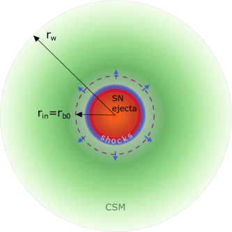
Figure 1: Sketch of the considered spherically symmetric geometry after the SN explosion. The outer edge of the CSM is marked as $r_{\rm w}$. The dashed magenta line marks the position of the radiation-mediated shock breakout ($r_{\rm in}=r_{\rm bo}$). The interaction of the SN ejecta (dark red colored region) with the CSM (light green colored region) leads to the formation of shocks that propagate radially outwards. The color gradient represents the density gradient of the CSM. The light red and blue colored regions represent, respectively, the shocked SN ejecta and the shocked CSM.

If $\mu$ is the mean number of nucleons per particle in the CSM, then the respective number density can be expressed as $n_{\rm csm}(r)=\rho_{\rm csm}(r)/\mu m_{\rm p}$. The Thomson optical depth due to photon scattering by electrons in the CSM is given by

$$\tau_{T}=\int_{r}^{r_{\rm w}}{\rm d}r^{\prime}n_{\rm e}(r^{\prime})\sigma_{T}\approx\frac{\sigma_{T}\rho_{0}r_{\rm in}}{\mu_{\rm e}m_{\rm p}(w-1)}\left(\frac{r_{\rm in}}{r}\right)^{w-1}.$$ (3)

where $\mu_{\rm e}$ is the mean number of electrons per particle and $r_{\rm w}\gg r$. Henceforth, we adopt $\mu=\mu_{\rm e}=1$ for simplicity. If $\upsilon_{0}$ is the the shock velocity at the breakout radius, the requirement that $\tau_{T}\sim c/\upsilon_{0}$ at breakout together with eq. (3) leads to a useful expression relating $\rho_{0},\upsilon_{0}$ and $r_{\rm in}$ (see also Ofek et al., 2014b), namely

$$\rho_{0}\approx\frac{(w-1)m_{\rm p}c}{\sigma_{T}r_{\rm in}\upsilon_{0}}.$$ (4)

For the case of a wind CSM density profile, the expected mass loading parameter is

$$A_{\rm w}\approx 10^{16}\,r_{\rm in,13}\,\beta^{-1}_{0,{-1.5}}\nobreak{\mathrm{\;gr\ cm}}^{-1},$$ (5)

where $\beta_{0}\equiv\upsilon_{0}/c$ was assumed. As the breakout time of the SN shock and its respective velocity are the parameters to be first determined by SNe observations, we will treat as primary model parameters $r_{\rm in}$ and $\upsilon_{0}$ rather than $\rho_{0}$ (or, $A_{\rm w}$ in the case of a wind density profile). For compact stars with tenuous fast winds the shock breakout may happen close to the progenitor radius, i.e. $r_{\rm in}\sim$ a few times $10^{11}$ cm (see Waxman et al., 2007). For progenitors with high mass-loss rates, however, the shock breakout is expected to take place in the wind and well outside the progenitor, i.e. $r_{\rm in}\sim 10^{13}-10^{14}$ cm (see Rabinak & Waxman, 2011; Chevalier, 2012).

The ejecta-CSM interaction leads eventually to the formation of a shell with high internal energy density (e.g. Chevalier, 1982; Chevalier & Fransson, 1994; Truelove & McKee, 1999), whose equation of motion was studied by Chevalier (1982) for the case of spherically expanding SN ejecta with a power-law density profile, i.e. $\rho_{\rm SN}\propto r^{-n_{\rm sn}}$. The density profiles of both the SN ejecta and the CSM are necessary for detailed calculations, since the time evolution of the shock front radius and velocity $\upsilon_{\rm s}$ depends on these. For the purposes of our study it is sufficient to assume that the shock velocity has a radial power-law profile of the form

$$\upsilon_{\rm s}(r)=\upsilon_{0}\left(\frac{r}{r_{\rm in}}\right)^{\alpha},$$ (6)

The power-law index $\alpha\leq 0$ can be written in terms of the power-law indices of the CSM and SN ejecta density profiles (e.g. Ofek et al., 2014b). Typically, the forward shock is expected to be mildly decelerating, unless the SN ejecta have a flat density profile ($n_{\rm sn}<3$) (e.g. Chevalier, 1982; Tan et al., 2001). For example, $\alpha=-0.1$ for a wind-like CSM ($w=2$) and ejecta with $n_{\rm sn}=12$, whereas if both media are uniform the SN shock propagates with a constant velocity, at least in the free expansion phase (e.g. Matzner & McKee, 1999). To keep our analysis as general as possible, we will treat the index $\alpha$ as a free parameter. Table 1 summarizes the free parameters of the model.

Table 1: Free model parameters and their default values used in the text.

Parameter	Symbol	Default value
Input
Power-law index of the CSM density profile	$w$	2
Power-law index of the shock velocity profile	$\alpha$	0
Power-law index of the SN luminosity profile	$a_{\rm ph}$	0
Power-law slope of shock accelerated particles	$s$	2
Magnetic energy density fraction	$\epsilon_{\rm B}$	$10^{-2}$
Accelerated proton energy fraction	$\epsilon_{\rm p}$	$10^{-1}$
Electron-to-proton ratio	$K_{\rm ep}$	$10^{-3}$
Peak supernova luminosity (erg s-1)	$L_{\rm sn,pk}$	$10^{41}$
Breakout radius (cm)	$r_{\rm in}$	$10^{13}$
Shock velocity at breakout radius	$\upsilon_{0}$	0.03 c
Wind velocity	$\upsilon_{\rm w}$	$0.01$ c
Electron temperature of unshocked CSM (K)	$T_{\rm e}$	$10^{5}$
Output
$a_{\rm B}$	$w/2-\alpha$	1
$q_{\rm syn}$	$2a_{\rm B}+\alpha$	2
$q_{\rm ic}$	$2+a_{\rm ph}+\alpha$	2
$q_{\rm pp}$	$w-1+\alpha$	1

The free expansion phase of the SN ejecta lasts until the mass in the ejecta $M_{\rm ej}$ is comparable to the swept-up mass $M_{\rm sw}$. The transition from the free expansion phase to the so-called Sedov-Taylor phase will happen at a radius

$$r_{\rm dec}=r_{\rm in}\left[\frac{(3-w)M_{\rm ej}}{4\pi\rho_{0}r_{\rm in}^{3}}\right]^{1/(3-w)}.$$ (7)

The above equation is valid as long as $r_{\rm in}\ll r_{\rm dec}$ and $w<3$. For the case of the wind, the deceleration radius may be written as

$$r_{\rm dec}=\frac{M_{\rm ej}}{A_{\rm w}}\simeq{1.8\times 10^{18}}\,M_{\rm ej,1}\,\beta_{0,{-1.5}}\,r_{\rm in,13}^{-1}\nobreak{\mathrm{\;cm}}$$ (8)

where we used eq. (2) and eq. (5). In the above, $M_{\rm ej,1}\equiv M_{\rm ej}/{10}M_{\odot}$. For typical parameters, we thus find $r_{\rm dec}\simeq 0.3-3$ pc; these distances are much larger than the characteristic shock radii that we will consider in this work.

In the present work we will focus on the acceleration and non-thermal emission from the forward shock. As long as the density profile of the ejecta is steep, the contribution of the reverse shock to the observed non-thermal radiation is expected to be small (Chevalier & Fransson 2003; see also Fig. 3 in Zirakashvili & Ptuskin 2015). We further assume that all the material accreted by the forward shock is confined in a thin homogeneous layer downstream of the forward shock (e.g. Chevalier, 1982; Sturner et al., 1997). At the early stages of the SN expansion, the forward shock is expected to have Mach numbers $\gg 1$. We therefore assume that the compression ratio is $\approx 4$ (e.g. Sturner et al., 1997) and the width of the shock is then 25% of the shock radius. The latter is in rough agreement with the findings of recent hydrodynamic calculations of the shock structure (Zirakashvili & Ptuskin, 2015). Similarly, Chevalier (1982) found that for steep density profiles of the SN ejecta ($n_{\rm sn}=7-12$) the width of the shocked CSM at radius $r$ is $h\sim 0.2\,r$.

Under these considerations, the average density of the shocked CSM is a factor of four larger than the upstream CSM density at that radius, i.e. $n(r)=4\,n_{\rm csm}(r)$ or

$$n(r)=n_{0}\left(\frac{r_{\rm in}}{r}\right)^{w},$$ (9)

with $n_{0}\equiv 4\rho_{0}/m_{\rm p}$. For a wind-type medium this reduces to

$$n(r)\simeq{2\times 10^{13}}\,r_{\rm in,13}^{-1}\,\beta_{0,{-1.5}}^{-1}\left(\frac{r_{\rm in}}{r}\right)^{2}\nobreak{\mathrm{\;cm}}^{-3}.$$ (10)

Strictly speaking, the Rankine-Hugoniot jump conditions across a strong shock determine the particle density right behind the shock as a function of the upstream properties. Here, we assume the same scaling for the volume-averaged post-shock density.

For the calculation of the synchrotron emission, an estimate of the post-shock magnetic field strength is required. We assume that the magnetic energy density in the shell of shocked CSM is a fixed fraction $\epsilon_{\rm B}$ of the post-shock thermal energy density, which is written as $U_{\rm th}(r)=(9/32)m_{\rm p}\upsilon_{\rm s}^{2}(r)n(r)$. Here, we considered that the upstream speed in the post-shock frame is $3\,\upsilon_{\rm s}/4$, so the mean post-shock energy per particle is $(9/16)m_{\rm p}\upsilon_{\rm s}^{2}/2$. The magnetic field strength is therefore given by

$$B(r)=B_{0}\left(\frac{r_{\rm in}}{r}\right)^{a_{\rm B}},$$ (11)

where $a_{\rm B}=w/2-\alpha$ and $B_{0}\equiv(3/2)\sqrt{\pi\epsilon_{\rm B}m_{\rm p}n_{0}\upsilon_{0}^{2}}$. For a wind CSM density profile, the magnetic field is written as

$$B(r)\simeq{1.4\times 10^{3}}\,\epsilon_{\rm B,-2}^{1/2}r_{\rm in,13}^{-1/2}\beta_{0,{-1.5}}^{1/2}\left(\frac{r_{\rm in}}{r}\right)\nobreak{\mathrm{\;G}},$$ (12)

where we used eq. (10) and $\beta_{0}\equiv\upsilon_{0}/c$, while $\epsilon_{\rm B}$ is considered a free parameter of the model. Typical values inferred from radio observations of interaction-powered SNe lie in the range $\epsilon_{\rm B}\sim 10^{-2}-10^{-1}$ (Chevalier, 1998; Björnsson & Fransson, 2004; Chevalier & Fransson, 2006; Kamble et al., 2015b), in contrast to GRB afterglows where $\epsilon_{\rm B}\ll 10^{-2}$ are usually inferred from the observations (Santana et al., 2014; Barniol Duran, 2014; Zhang et al., 2015). We note that at times relevant for $\sim$GHz radio observations the magnetic field strength has already reached $\sim$G values:

$$B\simeq 3.6\,\epsilon_{\rm B,-2}^{1/2}r_{\rm in,13}^{1/2}A_{\rm w,16}^{3/2}\beta_{\rm 0,-1.5}^{1/2}T_{\rm e,5}^{1/2}\nu_{\rm obs,9}^{2/3}\nobreak{\mathrm{\;G}},$$ (13)

where $T_{\rm e}$ is the electron temperature of the unshocked CSM and $\nu_{\rm obs}$ is the observing frequency.

2.1 The injection of primary particles

In this section we determine the injection distributions of primary electrons and protons, focusing only on relativistic particles. We assume that a fraction of the incoming particles at the SN shock will be accelerated into a power-law distribution in energy, with the nature of the acceleration process itself not being crucial for the present study. CR that have accelerated at the shock front will subsequently escape in the donwstream region of the shock where they will lose energy via various physical processes (see below). It is in this region where the production of secondary particles due to pp collisions takes place (see e.g. Mastichiadis, 1996; Sturner et al., 1997).

If $s$ is the power-law index of the distribution, the injection function for both primary electrons and protons, i.e. the number of relativistic particles injected in the shell per unit Lorentz factor and per unit radius, $Q_{\rm i}(\gamma,r)\equiv{\rm d}^{2}N_{\rm i}/{\rm d}\gamma{\rm d}r$, can be written as

$$Q_{\rm i}(\gamma,r)=Q_{\rm 0i}\,g_{\rm i}(r)\,\gamma^{-s}H[\gamma-\gamma_{\rm i,m}]H[\gamma_{\rm i,M}-\gamma]$$ (14)

where ${\rm i=e,p}$, $H[x]=1$ for $x>0$ and 0 otherwise, $g_{\rm i}$ is an arbitrary function of radius, and $\gamma_{\rm i,m},\gamma_{\rm i,M}$ are the minimum and maximum Lorentz factors of particles at injection (to be specified below). The exact value of the power-law index depends on the details of shock acceleration, such as non-linear effects at the shock front and shock obliquity (e.g. Jones & Ellison, 1991, and references therein), which are not treated in this study. Thus, we will consider $s$ to be a free parameter of the model and assume that is the same for electrons and protons. We remark that the formalism we present below does not hold only for a power-law injection function, but it can be applied to injection distributions with an arbitrary dependence on energy.

2.1.1 The injection rate and minimum energy at injection

The normalization factor $Q_{\rm 0i}$ can be determined based on recent kinetic simulations, that can capture the acceleration of protons at non-relativistic shocks from first principles (e.g. Caprioli & Spitkovsky, 2014a; Park et al., 2015). It has been found that, if the shock is quasi-parallel, i.e., the magnetic field in the upstream is nearly aligned (within $\lesssim 45^{\circ}$) with the direction of shock propagation, a fraction $\epsilon_{\rm p}\sim 5-10\%$ of the shock energy is channeled into relativistic protons ($\gamma\gtrsim 2$). In the following, we assume $\epsilon_{\rm p}$ to be constant in time and treat it as a free parameter (see also Appendix A). The incoming kinetic energy per unit radius is $\mathcal{E}_{\rm k}=(9\pi/32)m_{\rm p}\upsilon_{\rm s}^{2}(r)\,r^{2}n(r)$, where we used the same considerations as for the derivation of $U_{\rm th}$. From the requirement that relativistic protons acquire a fraction $\epsilon_{\rm p}$ of the incoming energy per unit radius, we can determine the normalization $Q_{\rm 0p}$ as

$$Q_{\rm 0p}=\frac{9\pi}{32}\epsilon_{\rm p}r_{\rm in}^{2}\,n_{0}\beta_{0}^{2}\left\{\begin{array}[]{cc}(s-2),&s>2\\ \\ \ln^{-1}\left(\frac{\gamma_{\rm p,M}}{\gamma_{\rm p,m}}\right),&s=2\end{array}\right.$$ (18)

and the radial dependence of the injection rate as

$$g_{\rm p}(r)=\left(\frac{r}{r_{\rm in}}\right)^{2\alpha+2-w}$$ (19)

The above relations are derived using eqs. (6) and (9) under the assumptions of $\gamma_{\rm p,M}\gg\gamma_{\rm p,m}$ and $\gamma_{\rm p,m}=2$ (see also Appendix A). In the case of a wind-like CSM ($w=2$) and constant shock velocity ($\alpha=0$) the injection rate is constant, i.e. $g_{\rm p}=1$.

Unlike protons, shock-accelerated electrons are all likely to be ultra-relativistic, which is indeed consistent with modeling the radio emission signature of interaction-powered supernovae: SN 2009ip (Margutti et al., 2014), SN 2010jl (Fransson et al., 2014; Ofek et al., 2014b), SN 1988Z (Chugai & Danziger, 1994), and 2006jd (Chandra et al., 2012). Assuming energy equipartition between thermal post-shock electrons and protons, we find that the Lorentz factor of thermal electrons is

$$\gamma_{\rm th,e}(r)\simeq\frac{9}{64}\frac{m_{\rm p}}{m_{\rm e}}\left(\frac{\upsilon_{\rm s}(r)}{c}\right)^{2}\simeq 2.5\beta_{0,-1}^{2}\left(\frac{r}{r_{\rm in}}\right)^{2\alpha},$$ (20)

where here the shock velocity was normalized to $0.1c$. Because of the quadratic dependence on the shock velocity, the thermal electrons turn out to be non-relativistic at slower shocks. Recent particle-in-cell (PIC) simulations (e.g. Park et al., 2015; Guo et al., 2014a, b) show that the minimum momentum of the electron distribution is three times larger than the thermal one. For our calculations, we will therefore adopt $\gamma_{\rm e,m}=3\gamma_{\rm e,th}$, if the latter is mildly relativistic (see eq. (20)). Otherwise, we will assume that $\gamma_{\rm e,m}=1$ (see also Appendix A).

For the electron normalization, we adopt the common assumption that the ratio of the electron to proton spectrum at a given energy $E\gg m_{p}c^{2}$ is $K_{\rm ep}$, namely

$$K_{\rm ep}=\frac{Q_{\rm e}\left(\frac{E}{m_{\rm e}c^{2}},r\right)}{Q_{\rm p}\left(\frac{E}{m_{\rm p}c^{2}},r\right)}\frac{m_{\rm p}}{m_{\rm e}},$$ (21)

with $K_{\rm ep}$ ranging typically between $10^{-3}-5\times 10^{-3}$ according to PIC simulations (e.g. Park et al., 2015). These values are in rough agreement with those inferred from observations. A value of $K_{\rm ep}\simeq 0.01$ is determined by direct measurements of cosmic-rays at Earth at 10 GeV (e.g. Cohen & Ramaty, 1973; Picozza et al., 2013). Observations of young SN remnants at X-ray and GeV $\gamma$-rays imply $K_{\rm ep}\lesssim 10^{-3}$ (e.g. Völk et al., 2005; Morlino & Caprioli, 2012; Yuan et al., 2012), although somewhat higher values $\sim 0.01$ have also been reported (e.g. Gaisser et al., 1998). In the following, we adopt $K_{\rm ep}=10^{-3}$ as the default value (see Table 1). The above expression leads finally to

$$Q_{\rm 0e}=K_{\rm ep}\left(\frac{m_{\rm p}}{m_{\rm e}}\right)^{s-1}Q_{\rm 0p},$$ (22)

while the radial dependence of the electron injection function is the same as for the protons, namely $g_{\rm e}(r)=g_{\rm p}(r)$.

2.1.2 The maximum energy at injection

The maximum energy of particles being accelerated at the shock is determined by the competition of acceleration and various cooling as well as loss processes (e.g. Gaisser, 1990; Mastichiadis, 1996; Sturner et al., 1997). In this paragraph, we estimate the maximum Lorentz factor of accelerated electrons and protons by comparing the relevant acceleration timescales with the dynamical and cooling timescales.

• Acceleration timescale: the scattering at the basis of the Fermi acceleration process is usually assumed to proceed in the Bohm limit, leading to $t_{\rm acc,i}\sim 6\gamma m_{\rm i}c^{3}/eB\upsilon_{\rm s}^{2}$ (e.g. Protheroe & Clay, 2004; Rieger et al., 2007; Tammi & Duffy, 2009).

• Dynamical timescale: by requiring that the acceleration timescale is shorter than the dynamical timescale $t_{\rm dyn}(r)\sim r/\upsilon_{\rm s}$ (which is the typical timescale of adiabatic losses) we derive

  $$\gamma_{\rm i,M}^{(1)}(r)=\frac{eB_{0}\beta_{0}r_{\rm in}}{6m_{\rm i}c^{2}}\left(\frac{r}{r_{\rm in}}\right)^{1-a_{\rm B}+\alpha},$$ (23)

  which is independent of the shock radius for $a_{\rm B}=1$ and $\alpha=0$. As $t_{\rm dyn}$ is also a measure of the age of the system, we will refer to this criterion as the “age criterion”. For the wind CSM density profile and typical parameter values, we find that the age constraint limits the maximum particle Lorentz factor to

  $$\gamma^{(1)}_{\rm i,M}{m_{\rm i}c^{2}}\simeq{1.2\times 10^{16}\nobreak{\mathrm{\;eV}}}\,\epsilon_{\rm B,-2}^{1/2}\,\beta_{0,{-1.5}}^{2}A_{\rm w,{16}}^{1/2}$$ (24)

  where we used eq. (12), while $A_{\rm w}$ is related to $\beta_{0}$, $r_{\rm in}$ through eq. (5). Protons in the shocks of type IIn SNe can, in principle, achieve multi-PeV energies due to the high-density CSM, as it has been already noted by Katz et al. (2011); Murase et al. (2011, 2014); Zirakashvili & Ptuskin (2015).

  The age criterion is closely related to the so-called confinement criterion, which requires the particle gyro-radius to be smaller than the maximum wavelength $\lambda_{\max}$ of the scattering turbulence, to avoid the particle escape from the acceleration region. If $\lambda_{\max}\sim r$, the respective maximum Lorentz factor is larger by a factor of $c/\upsilon_{\rm s}$ than that derived from the age criterion. In this regard, the age criterion is more constraining. However, if $\lambda_{\max}\ll r$, then the maximum proton energy may be limited to energies much below the PeV energy range, as it has been recently demonstrated by Metzger et al. (2016) for the case of gamma-ray novae. The cosmic-ray confinement is non-trivial, since it depends on the details of the acceleration process, the magnetic field amplification and the ionization properties of the upstream medium. The exact value of the maximum particle energy is not crucial for the purposes of the present study. Thus, eq. (24) will be used in the following.

• Cooling timescales: the most relevant cooling processes for relativistic electrons are synchrotron and inverse Compton (IC) scattering energy losses. The corresponding losses for relativistic protons are negligible. Inelastic pp collisions and photohadronic interactions (photopion and photopair production) are the most relevant processes for determining the maximum energy of relativistic protons (e.g. Katz et al., 2011; Murase et al., 2011). Coulomb and bremsstrahlung energy losses become important only at low energies and do not play role in setting the maximum particle energy.

  1. Synchrotron cooling: by setting $t_{\rm acc,e}=t_{\rm syn}$, where $t_{\rm syn}(\gamma,r)=6\pi m_{\rm e}c/\sigma_{T}\gamma B^{2}(r)$, we derive the respective maximum electron Lorentz factor. For the general case, this is given by

     $$\gamma_{\rm e,M}^{(2)}(r)=\left(\frac{\pi e\beta_{0}^{2}}{\sigma_{T}B_{0}}\right)^{1/2}\left(\frac{r}{r_{\rm in}}\right)^{a_{\rm B}/2+\alpha}$$ (25)

     and reduces to the expression below for a wind CSM density and constant shock velocity

     $$\gamma_{\rm e,M}^{(2)}(r)\simeq{3.8}\times 10^{4}\,\beta_{0,{-1.5}}^{1/2}\,r_{\rm in,13}^{1/2}\epsilon_{\rm B,-2}^{-1/4}A_{\rm w,{16}}^{-1/4}\left(\frac{r}{r_{\rm in}}\right)^{1/2}.$$ (26)

  2. Inverse Compton cooling: relativistic electrons also lose energy due to IC scattering of soft photons provided by the SN. To take into account a possible decay of the SN luminosity with time (or radius) we model the SN luminosity as $L_{\rm SN}=L_{\rm SN,pk}(r_{\rm in}/r)^{a_{\rm ph}}$ with $a_{\rm ph}\geq 0$. The energy density of the SN photon field in the shell is then written as

     $$U_{\rm ph}=\frac{L_{\rm SN}}{4\pi c(r+h)^{2}}\approx U_{0}\left(\frac{r_{\rm in}}{r}\right)^{2+a_{\rm ph}}$$ (27)

     where $U_{0}=L_{\rm SN,pk}/4\pi cr_{\rm in}^{2}$. We note that ambient photon fields, such as the cosmic microwave background and the galactic optical/infrared photon fields, are not included in the present analysis, since their energy density is typically lower than that given in eq. (27). For example, if $L_{\rm SN}=$const $\sim 10^{41}$ erg s^-1, the energy density of SN photons is higher than that of ambient photon fields as long as $r\lesssim 0.3$ kpc (see also Gaisser et al. 1998). Assuming that the IC scattering takes place in the Thomson regime, the maximum electron Lorentz factor is given by

     $$\gamma_{\rm e,M}^{(3)}(r)=\left(\frac{e\beta_{0}^{2}B_{0}}{8\sigma_{T}U_{0}}\right)^{1/2}\left(\frac{r}{r_{\rm in}}\right)^{(2+a_{\rm ph}-a_{\rm B}+2\alpha)/2}.$$ (28)

     which, for the case of wind-type medium, constant shock velocity and SN luminosity, simplifies to

     $$\gamma_{\rm e,M}^{(3)}(r)\simeq{3\times 10^{5}}\,\beta_{0,{-1.5}}^{3/2}\epsilon_{\rm B,-2}^{1/4}A_{\rm w,{16}}^{1/4}r_{\rm in,13}^{1/2}L_{\rm sn,pk,41}^{-1/2}\left(\frac{r}{r_{\rm in}}\right)^{1/2}.$$ (29)

     The above hold as long as the IC scatterings take place in the Thomson regime. However, the Klein-Nishina suppression of the scattering rate becomes important for $\gamma\gtrsim m_{\rm e}c^{2}/\epsilon_{\rm ph}$, or $\gamma\gtrsim 5\times 10^{5}$ for $\epsilon_{\rm ph}=1$ eV, which is the typical photon energy for the SN emission. Although the Klein-Nishina suppression may be not relevant for primary electrons, the IC scatterings of optical photons by secondary electrons will take place deep in the Klein-Nishina regime (see Sect. 3 for more details).

     At each shock radius, the highest energy electrons will be injected with a Lorentz factor $\gamma_{\rm e,M}=\min[\gamma_{\rm e,M}^{(1)},\gamma_{\rm e,M}^{(2)},\gamma_{\rm e,M}^{(3)}]$. In general, synchrotron (and IC) cooling will dominate at early times, whereas the age criterion becomes relevant at larger shock radii, where both the magnetic and photon field energy densities have considerably decreased.

  3. Inelastic pp collision losses: let us consider next the effect of pp collisions on the accelerated protons. The corresponding timescale is

     $$t_{\rm pp}\simeq\left(\kappa_{\rm pp}\sigma_{\rm pp}n(r)c\right)^{-1}$$ (30)

     where we assumed a constant inelasticity $\kappa_{\rm pp}\simeq 0.5$ and neglected the weak energy-dependence of the cross section $\sigma_{\rm pp}\simeq 3\times 10^{-26}$ cm²; however, the energy-dependent cross section is taken into account in our numerical calculations (for more details, see Sect. 3). In eq. (30) it is the density of the shocked CSM that appears, since pp collisions are assumed to take place in the post-shock region. By requiring that $t_{\rm acc,p}=t_{\rm pp}$, we find that the maximum proton Lorentz factor is limited to

     $$\gamma_{\rm p,M}^{(2)}=\frac{eB_{0}\beta_{0}^{2}}{6\kappa_{\rm pp}\sigma_{\rm pp}n_{0}m_{\rm p}c^{2}}\left(\frac{r}{r_{\rm in}}\right)^{w-a_{\rm B}+2\alpha}$$ (31)

     which increases linearly in radius for a shock propagating with a constant velocity in a wind-like CSM, namely

     $$\gamma_{\rm p,M}^{(2)}\simeq{2.7\times 10^{5}}\,\beta_{0,{-1.5}}^{3}r_{\rm in,13}A_{\rm w,{16}}^{-1/2}\left(\frac{r}{r_{\rm in}}\right)$$ (32)

     Inspection of eqs. (24) and (32) shows that pp losses dominate over adiabatic proton cooling at small radii, but since the former increases with radius, the maximum energy of protons at later times is set by the age criterion.

  4. Photohadronic energy losses: in the presence of photon fields, energetic protons may lose energy through photohadronic interactions. Although the energy threshold for photopion production on $\epsilon_{\rm ph}=1$ eV photons is high ($\gamma_{\rm p,p\pi}\gtrsim m_{\pi}c^{2}/\epsilon_{\rm ph}\simeq 1.5\times 10^{8}/(\epsilon_{\rm ph}/1\,{\rm eV})$) and thus not relevant for our study, protons with Lorentz factors $\gamma_{\rm p,BH}\gtrsim m_{\rm e}c^{2}/\epsilon_{\rm ph}=5\times 10^{5}/(\epsilon_{\rm ph}/1\,{\rm eV})$ may lose energy through Bethe-Heitler pair production. It can be shown that the respective timescale, which can be recast in a similar form as $t_{\rm pp}$ (see Appendix B), is the longest one for a wide range of parameter values and can be safely neglected. Same as for the electrons, the maximum proton Lorentz factor at injection will be $\gamma_{\rm p,M}=\min[\gamma_{\rm p,M}^{(1)},\gamma_{\rm p,M}^{(2)}]$.

2.2 The injection of secondary electrons

Secondary electrons are the by-product of charged pion decays, i.e. $\pi^{\pm}\rightarrow\mu^{\pm}+\nu_{\mu}(\bar{\nu}_{\mu})$ and $\mu^{\pm}\rightarrow e^{\pm}+\bar{\nu}_{\mu}(\nu_{\mu})+\nu_{\rm e}(\bar{\nu}_{\rm e})$. Their injection rate ($Q_{\rm e}^{(\rm pp)}$) depends on the number density of “thermal” (i.e., non-relativistic) protons that are the targets for pp collisions, or equivalently on $n(r)$, and on the distribution of accelerated protons, that evolves as the shock propagates in the CSM. Thus, the evolution of the proton distribution is necessary for the calculation of the injection rate $Q_{\rm e}^{(\rm pp)}$. Aim of this paragraph is to derive a rough estimate of the ratio $Q_{\rm e}^{(\rm pp)}/Q_{\rm e}$ and investigate its dependence on the model parameters, such as $A_{\rm w}$. An accurate treatment of the secondary injection distributions will be presented in Sect. 7, where we employ the expressions by Kelner et al. (2006).

2.2.1 The injection rate

As an indicative example we assume a power-law proton distribution of the form $N_{\rm p}(\gamma,r)=Q_{\rm 0p}\,r\,\gamma^{-s}\,H[\gamma_{\rm p,M}-\gamma]H[\gamma-\gamma_{\rm p,m}]$, where the radial dependence is relevant to the case of a wind-type CSM and a constant shock velocity (for the general case of $w\neq 2$ and $\alpha\neq 0$, see Appendix C). We furthermore use approximate expressions for the pion production rate, as presented in Mannheim & Schlickeiser (1994). The following calculations are based on several assumptions that we list for clarity:

• we ignore the (weak) energy dependence of the pp cross section, i.e. $\sigma_{\rm pp}\simeq 3\times 10^{-26}$ cm².

• the multiplicity of pion production is taken to be $\xi\sim 1/3$ independent of the proton energy in the laboratory frame.

• for a single proton, the rate of increase of pion energy is approximated by a $\delta$-function centered at the average pion energy $\langle E_{\pi}\rangle\simeq(1/6)E_{\rm k,p}$, where $E_{\rm k,p}=E_{\rm p}-m_{\rm p}c^{2}$ is the proton kinetic energy

  $$\frac{{\rm d}E_{\pi}}{{\rm d}t}=1.3\sigma_{\rm pp}cn\xi E_{\pi}\delta\left(E_{\pi}-\langle E_{\pi}\rangle\right),$$ (33)

  for $E_{\rm p}>E_{\rm p,thr}\simeq 1.2$ GeV and the factor 1.3 accounts for the chemical composition of the matter.

• the secondary electron injection rate is given by

  $$Q_{\rm e}^{(\rm pp)}(\gamma)\equiv\frac{{\rm d}N_{\rm e}^{(\rm pp)}}{{\rm d}r{\rm d}\gamma}=\frac{1}{A}Q_{\pi}\left(\frac{\gamma}{A}\right)$$ (34)

  where $A=70\simeq m_{\pi}/(4m_{\rm e})$.

The pion injection rate for a proton distribution is then given by

$$Q_{\pi}(\gamma_{\pi})\equiv\frac{{\rm d}N_{\pi}}{{\rm d}r{\rm d}\gamma_{\pi}}\simeq\frac{m_{\pi}c^{2}}{E_{\pi}\upsilon_{\rm s}}\int_{1}^{\infty}\!\!{\rm d}\gamma N_{p}(\gamma,r)\frac{{\rm d}E_{\pi}}{{\rm d}t},$$ (35)

where we made use of $\upsilon_{\rm s}={\rm d}r/{\rm d}t$ and neglected the factor 1.26 that accounts for contributions from $\alpha-p$ and $\alpha-\alpha$ collisions (Mannheim & Schlickeiser, 1994). Using eq. (33) we find

$$Q_{\pi}(\gamma_{\pi})\simeq\frac{2.5\sigma_{\rm pp}nc}{\upsilon_{\rm s}}\frac{m_{\pi}}{m_{\rm p}}N_{\rm p}\left(6\gamma_{\pi}\frac{m_{\pi}}{m_{\rm p}}+1,r\right),$$ (36)

for pions with Lorentz factors in the range

$$\frac{m_{\rm p}}{6m_{\pi}}\gamma_{\rm p,thr}\leq\gamma_{\pi}\lesssim\frac{m_{\rm p}}{6m_{\pi}}\gamma_{\rm p,M},$$ (37)

where $\gamma_{\rm p,thr}=E_{\rm p,thr}/m_{\rm p}c^{2}\simeq 1.22$. Finally, using eq. (34) and substitution of $N_{\rm p}(\gamma,r)$ we find

$$Q_{\rm e}^{(\rm pp)}(\gamma,r)\simeq\left(\frac{m_{\rm e}}{m_{\rm p}}\right)^{-s+1}\frac{10Q_{\rm 0p}\sigma_{\rm pp}n(r)rc}{\upsilon_{\rm s}(r)}\left(24\gamma\right)^{-s}$$ (38)

for electron Lorentz factors in the range

$$\frac{m_{\rm p}}{24m_{\rm e}}\gamma_{\rm p,thr}\leq\gamma\lesssim\frac{m_{\rm p}}{24m_{\rm e}}\gamma_{\rm p,M},$$ (39)

where $\gamma_{\rm p,M}$ is, in principle, a function of radius. Thus, the typical Lorentz factor of the injected secondary electrons is

$$\gamma_{\rm e}^{(\rm pp)}\simeq\frac{\gamma_{\rm p}m_{\rm p}}{24m_{\rm e}}.$$ (40)

Using eq. (38) and eq. (22) the ratio of secondary to primary injection rates at a given Lorentz factor is written as (here, we generalize to any values of $w$ and $\alpha$)

$$\frac{Q_{\rm e}^{(\rm pp)}}{Q_{\rm e}}=24^{-s}\frac{10\sigma_{\rm pp}n_{0}r_{\rm in}}{\beta_{0}K_{\rm ep}}\left(\frac{r}{r_{\rm in}}\right)^{1-w-\alpha},$$ (41)

where we made use of eqs. (9) and (6). The injection ratio is a decreasing function of radius for $w=2$ and $\alpha\lesssim 0$, suggesting that the contribution of the secondaries to the synchrotron emission from the SN shock is expected to be most important at small radii. Interestingly, if the shock propagates in a thick CSM shell with uniform (high) density ($w=0$), then the ratio of secondary to primary electrons will increase as the shock propagates, provided that it is not significantly decelerated. Plugging into eq. (41) typical values for the parameters, as well as $w=2$ and $\alpha=0$, we find

$$\frac{Q_{\rm e}^{(\rm pp)}}{Q_{\rm e}}\simeq{3\times 10^{3}}\,A_{\rm w,{16}}r_{\rm in,13}^{-1}K^{-1}_{\rm ep,-3}\beta_{0,{-1.5}}^{-1}\left(\frac{r_{\rm in}}{r}\right),$$ (42)

or

$$\frac{Q_{\rm e}^{(\rm pp)}}{Q_{\rm e}}\simeq{3\times 10^{3}}\,K^{-1}_{\rm ep,-3}\beta_{0,{-1.5}}^{-2}\frac{r_{\rm in}}{r},$$ (43)

where we substituted $A_{\rm w}$ in the above expression using eq. (5). Interestingly, at $r=r_{\rm in}$ the ratio depends only on $K_{\rm ep}$ and the shock velocity. According to the above, slower shocks favour the production of secondaries, since the ratio ${Q_{\rm e}^{(\rm pp)}}/{Q_{\rm e}}$ increases. This result may seem counterintuitive at first sight but, in retrospect, it is not surprising. The ratio of injection between secondary and primary electrons will be proportional to $(Q_{\rm p}/Q_{\rm e})\times(t_{\rm age}/t_{\rm pp})\propto K^{-1}_{\rm ep}A_{\rm w}\beta_{0}^{-1}r^{-1}$, where $t_{\rm age}\sim r/\beta_{0}c$ is the age of the system. Slower shocks allow for pp interactions to act for a longer time, thus leading to a larger ${Q_{\rm e}^{(\rm pp)}}/{Q_{\rm e}}$ ratio.

2.3 The parameter space $A_{\rm w}-r$

In the case of wind CSM density profile, a parameter space of the mass loading parameter $A_{\rm w}$ versus the shock radius $r$ can be constructed using the following considerations:

1. Particle acceleration at radiation mediated shocks is suppressed (e.g. Waxman & Loeb, 2001; Katz et al., 2011). Roughly speaking, the shock is not radiation mediated if $\tau_{T}\lesssim c/\upsilon_{\rm s}$ or

   $$A_{\rm w}\leq\frac{4\pi m_{\rm p}cr_{\rm in}^{\alpha}}{\sigma_{T}\upsilon_{0}}r^{1-\alpha}$$ (44)

   where we used eqs. (3) and (6).

2. As the magnetic field in the shocked shell depends on the CSM density, it is expected that for high enough $A_{\rm w}$ values the magnetic energy density $U_{\rm B}$ in the shell will exceed that of the SN radiation field $U_{\rm ph}$. A lower limit on $A_{\rm w}$ can be derived by requiring $U_{\rm B}\geq U_{\rm ph}$, namely

   $$A_{\rm w}\geq\frac{8}{9}\frac{L_{\rm SN,pk}r_{\rm in}^{a_{\rm ph}+2\alpha}}{\epsilon_{\rm B}\beta_{0}^{2}c^{3}}r^{-a_{\rm ph}-2\alpha}.$$ (45)

   This should be considered as a strict lower limit, since it is derived for a SN optical light curve peaking at $r_{\rm in}$.

3. The emission from secondary electrons (at all energies) will be negligible, unless $Q_{\rm e}^{(\rm pp)}/Q_{\rm e}\gtrsim 1$. A ratio equal to unity corresponds to

   $$A_{\rm w}=24^{s}\frac{4\pi m_{\rm p}\beta_{0}K_{\rm ep}r_{\rm in}^{-\alpha}}{10\sigma_{\rm pp}}r^{1+\alpha},$$ (46)

   where we used eq. (41). In the following, we consider $0.1\leq Q_{\rm e}^{(\rm pp)}/Q_{\rm e}\leq 10$ as a range of values with possible interest for the secondary radiative signatures.

The parameter space $A_{\rm w}-r$ calculated for $\alpha=0$ and $a_{\rm ph}=0$ is presented in Fig. 2. The blue colored region denotes the parameter regime where a collisionless shock may be formed, thus allowing particle acceleration, and at the same time $U_{\rm B}\geq U_{\rm ph}$. The red colored region shows the parameter space where $1\leq Q_{\rm e}^{(\rm pp)}/Q_{\rm e}\leq 100$. For a given shock velocity at the breakout radius ($r_{\rm in}$), the value of the respective $A_{\rm w}$ can be read from the blue dashed line. Each horizontal line starting from a point $(A_{\rm w},r_{\rm in})$ and extending to $r_{\rm dec}$ (orange line) denotes the evolutionary path of the system that we will consider. Interestingly, the two different evolutionary paths shown in Fig. 2 have initially the same ratio of secondary to primary injection rates. As long as the shock breakout occurs in the CSM with a wind-like density profile, the ratio $Q_{\rm e}^{(\rm pp)}/Q_{\rm e}$ at $r=r_{\rm in}$ is independent of $A_{\rm w}$ and $r_{\rm in}$ (see also eq. (43)).

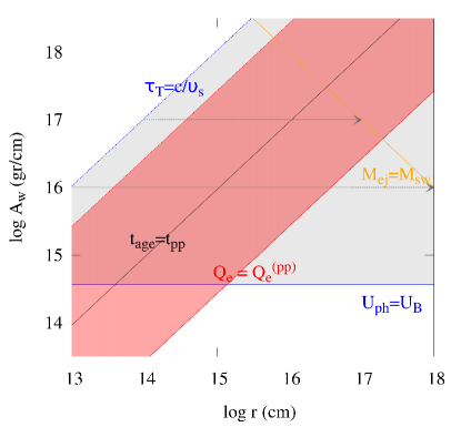
Figure 2: The $A_{\rm w}-r$ parameter space for a wind CSM density profile. The constraints eq. (44) and eq. (45) are shown with blue solid and dashed lines, respectively. The condition eq. (46) is plotted with a red solid line. A ratio $Q_{\rm e}^{(\rm pp)}/Q_{\rm e}$ equal to 1 and 100 corresponds to the red solid and dashed lines, respectively. The deceleration radius for different $A_{\rm w}$ (see eq. (7)) is overplotted with an orange line. The black solid line corresponds to $t_{\rm age}=t_{\rm pp}$. Each arrow (grey dashed line) denotes an “evolutionary path” of the system under consideration. Other parameters used: $L_{\rm sn,pk}=10^{41}$ erg s^-1, $M_{\rm ej}={10}M_{\odot}$, $K_{\rm ep}=10^{-3}$, $\epsilon_{\rm B}=0.01$, $\upsilon_{0}={0.03c}$, $\alpha=0$, $a_{\rm ph}=0$, and $s=2$.

The free model parameters and their values for the default case, that represents a SN shock propagating with a constant velocity in a wind-like CSM, are summarized in Table 1.

3 A semi-analytical framework for the particle evolution

In this section, we detail our semi-analytical formalism to solve for the evolution of the electron and proton spectrum (see also Finke & Dermer, 2012). This will be later applied to the early phases of SNe that expand in a CSM with non-uniform density profile. We stress, however, that the formalism we present here can be applied to a generic phase of supernova evolution and to an arbitrary power-law profile of the external medium.

We will be solving the evolutionary equations for protons and electrons (both primary and secondary) in the presence of losses and of a given injection term, which is provided by the particle escape downstream of the shock (e.g. Mastichiadis, 1996; Kirk et al., 1998). The general equation to be solved is

$$\frac{\partial\tilde{N}_{\rm i}}{\partial t}+\frac{\partial}{\partial\gamma}\left(\dot{\gamma}\tilde{N}_{\rm i}\right)=\tilde{Q}_{\rm i}(\gamma,t)$$ (47)

where $i=e,p$, $\dot{\gamma}\equiv{\rm d}\gamma/{\rm d}t$ is the energy loss term and $\tilde{N}_{\rm i}(\gamma,t)$ is the total number of particles in the shell at a given time $t$ with Lorentz factors between $\gamma$ and $\gamma+{\rm d}\gamma$. In the absence of the injection term on the right hand side and/or of a particle sink term on the left hand side, eq. (47) simply describes the conservation of the particle number. Spatial diffusion and advection are not considered here, since the shell is assumed to be homogeneous and all the material to be contained in the shell. Diffusion in momentum space due to moving Alfvén waves turns to be negligible and is, therefore, neglected.

It is more convenient to solve the equation above with respect to the shock radius $r$ instead of time $t$. Since ${\rm d}r/{\rm d}t=\upsilon_{\rm s}(r)$, where $\upsilon_{\rm s}$ is the shock velocity, the particle kinetic equation can be recast in the form

$$\frac{\partial N_{\rm i}}{\partial r}+\frac{\partial}{\partial\gamma}\left(\gamma^{\prime}\,N_{\rm i}\right)=Q_{\rm i}(\gamma,r),$$ (48)

where $\gamma^{\prime}\equiv{\rm d}\gamma/{\rm d}r$, $Q_{\rm i}(\gamma,r)\equiv{\tilde{Q}_{\rm i}(\gamma,t)}/{\upsilon_{\rm s}(r)}$ and $N_{\rm i}\equiv N_{\rm i}(\gamma,r)$. In the case where the particle-containing volume undergoes adiabatic expansion, it is the total number of particles $N_{\rm i}$ that should enter the equation above instead of the volume-averaged number density $n_{\rm i}\equiv{\rm d}^{2}N/{\rm d}V{\rm d}\gamma$. In fact, the volume-averaged number density $n_{\rm i}$ would not be conserved due to the volume expansion of the shell. The kinetic equation written in terms of differential particle densities would then read (to be contrasted with the commonly-used eq. (9) in Sturner et al. (1997))

$$\frac{\partial n_{\rm i}}{\partial r}+\frac{\partial}{\partial\gamma}\left(\gamma^{\prime}n_{\rm i}\right)+3\frac{n_{\rm i}}{r}=\frac{{Q}_{\rm i}(\gamma,r)}{V}$$ (49)

where the third term on the left hand side accounts for the expansion of the shell volume $V$. The following sections describing the semi-analytical formalism can be skipped from readers that are interested only in the astrophysical implications of our results (see Sect. 7). The method described below is also detailed in e.g. Stawarz et al. (2008) and Petropoulou & Mastichiadis (2009), albeit in a different context.

3.1 The proton distribution

The cooling term for relativistic protons due to adiabatic expansion is given by

$${\gamma^{\prime}}_{\rm ad}=-\frac{\gamma}{3}\,\frac{{\rm d}\ln V}{{\rm d}r}=-\frac{\gamma}{r},$$ (50)

where the volume of the shocked shell is $V\approx 4\pi r^{2}h$ and $h$ is the width of shell, which is assumed to be a fraction of the shock radius. Inelastic pp collisions can be approximated as catastrophic energy losses, since the proton in one collision loses a significant fraction ($\kappa_{\rm pp}$) of its energy (e.g. Sturner et al., 1997). In this approximation, the pp collisions are treated as an escape term in the kinetic equation of protons (eq. (48)), which is of the form $-N_{\rm p}/t_{\rm pp}$ (e.g. Schlickeiser, 2002). In this case, pp losses do not affect the evolution of the high-energy cutoff of the distribution (e.g. Mastichiadis & Kirk, 1995), but just the number of available protons. The energy loss terms due to photohadronic interactions are less important than the aforementioned cooling processes and can be safely neglected. For sufficiently high density in the shocked shell, trans-relativistic protons may also cool due to Coulomb collisions with background thermal electrons. However, at these low energies the exact shape of the proton distribution is not crucial, since their non-thermal emission is irrelevant to radio observations and the cross section for pp collisions decreases significantly. The evolution of the proton distribution function will follow

$$\frac{\partial N_{\rm p}}{\partial r}+\frac{\partial}{\partial\gamma}\left({\gamma^{\prime}}_{\rm ad}N_{\rm p}\right)+\frac{N_{\rm p}}{\upsilon_{\rm s}(r)t_{\rm pp}}=Q_{\rm p}(\gamma,r)$$ (51)

where $t_{\rm pp}$ is defined in eq. (30). In the case that the energy dependence of the source term can be described by a power law, i.e. $Q_{\rm p}\propto\gamma^{-s}$, the proton distribution is also a power law with the same exponent. The evolution of the proton Lorentz factor, which is governed by eq. (50), is written as

$$\gamma_{0}=\gamma\left(\frac{r}{r_{0}}\right).$$ (52)

In the absence of a source term, the solution to eq. (51) is

$$N_{\rm p}(\gamma,r)=N_{\rm p}(\gamma_{0},r_{0})\frac{\gamma_{0}}{\gamma}f_{\rm p}(r,r_{0}),$$ (53)

where $\gamma_{0}>\gamma$ is particle Lorentz factor at an arbitrary radius $r_{0}<r$ and

$$f_{\rm p}(r,r_{0})=\exp\left[-\frac{A_{\rm pp}}{q_{\rm pp}}\left(\frac{r_{\rm in}}{r_{0}}\right)^{q_{\rm pp}}\left(1-\left(\frac{r_{0}}{r}\right)^{q_{\rm pp}}\right)\right].$$ (54)

In the above we introduced $q_{\rm pp}=w-1+\alpha$ and

$$A_{\rm pp}=\frac{r_{\rm in}}{t_{\rm pp}\upsilon_{0}}\simeq 10(w-1)\,\beta_{0,-1}^{-2},$$ (55)

where we used eq. (4). The catastrophic pp losses reduce the number of protons in the source through the exponential term, while it does not affect the radial evolution of a single proton energy. Roughly speaking, the pp loss term will dominate the adiabatic loss term in eq. (51), if $r/r_{\rm in}\lesssim A_{\rm pp}^{1/q_{\rm pp}}\simeq[10(w-1)]^{1/q_{\rm pp}}\beta_{0,-1}^{-2/q_{\rm pp}}$. For the default case, where $q_{\rm pp}=1$, we find that the adiabatic losses will be controlling the proton evolution for $r\gtrsim 10r_{\rm in}$.

For a generic source term of protons, $Q_{\rm p}(\gamma,r)$ the proton distribution as a function of shock radius is given by

$$N_{\rm p}(\gamma,r)=\int_{r_{\min}}^{r}Q_{\rm p}(\gamma_{0},r_{0})\,\frac{\gamma_{0}}{\gamma}f_{\rm p}(r,r_{0})\,{\rm d}r_{0},$$ (56)

where $\gamma_{0}$ in the integral is considered a function of $r_{0},r$ and $\gamma$ (see eq. (52)). The lower integration limit, $r_{\min}$, depends on the injection radius as well as on the cooling history of particles (for details, see Appendix C).

3.2 The electron distribution

Besides cooling due to adiabatic expansion (see eq. (50)), relativistic electrons lose energy due to synchrotron radiation and IC scattering. Using eqs. (11) and (6) the synchrotron cooling term is written as

$$\gamma^{\prime}_{\rm syn}=\frac{1}{\upsilon_{\rm s}}\left(\frac{{\rm d}\gamma}{{\rm d}t}\right)_{\rm syn}=-K_{\rm syn}\frac{\gamma^{2}}{r_{\rm in}}\left(\frac{r_{\rm in}}{r}\right)^{2a_{\rm B}+\alpha}$$ (57)

where $K_{\rm syn}=\sigma_{T}B_{0}^{2}r_{\rm in}/(6\pi m_{\rm e}c\upsilon_{0})$ is a dimensionless constant and $q_{\rm syn}=2a_{\rm B}+\alpha$. For the calculation of the IC cooling term, we assume that the dominant photon field that is present in the shocked shell is the SN optical radiation. The IC scatterings between electrons and photons with characteristic energy $\epsilon_{\rm ph}=1$ eV take place in the Thomson regime, as long as $\gamma\lesssim\gamma_{\rm KN}\equiv m_{\rm e}c^{2}/\epsilon_{\rm ph}\sim 5\times 10^{5}$. For electrons with $\gamma<\gamma_{\rm KN}$ the IC cooling term reads, in complete analogy with eq. (57), as

$$\gamma^{\prime}_{\rm ic}=\frac{1}{\upsilon_{\rm s}}\left(\frac{{\rm d}\gamma}{{\rm d}t}\right)_{\rm ic}=-K_{\rm ic}\frac{\gamma^{2}}{r_{\rm in}}\left(\frac{r_{\rm in}}{r}\right)^{q_{\rm ic}}$$ (58)

where $K_{\rm ic}=4\sigma_{T}U_{0}r_{\rm in}/(3m_{\rm e}c\upsilon_{0})$ and $q_{\rm ic}=2+a_{\rm ph}+\alpha$. For $\gamma\gg\gamma_{\rm KN}$ the cooling rate is reduced due to the Klein-Nishina suppression of the cross section (e.g. Blumenthal & Gould, 1970). Although approximate expressions of the cooling rate that interpolate between the Thomson and Klein-Nishina regime can be found (e.g. Moderski et al., 2005), these do not allow for analytical solution of the electron kinetic equation. However, if the IC cooling is not important compared to other loss processes, then the complications of the Klein-Nishina effects can be ignored. Indeed, for dense CSM, where the emission signatures of secondary electrons will be important, synchrotron cooling is expected to dominate over IC cooling (see also Fig. 2). Thus, we may confidently use eq. (58), as long as the electrons cool predominantly due to synchrotron radiation (see condition eq. (45) and Fig. 2).

The evolution of the electron Lorentz factor $\gamma$ in radius, under the effect of adiabatic, synchrotron and IC losses is described by

$${\gamma^{\prime}}=-\frac{\gamma}{r}-K_{\rm syn}\frac{\gamma^{2}}{r_{\rm in}}\left(\frac{r_{\rm in}}{r}\right)^{q_{\rm syn}}-K_{\rm ic}\frac{\gamma^{2}}{r_{\rm in}}\left(\frac{r_{\rm in}}{r}\right)^{q_{\rm ic}}$$ (59)

which is conveniently rewritten as

$$\frac{{\rm d}[(\gamma r)^{-1}]}{{\rm d}r}=\frac{K_{\rm syn}}{r_{\rm in}^{2}}\left(\frac{r_{\rm in}}{r}\right)^{1+q_{\rm syn}}+\frac{K_{\rm ic}}{r_{\rm in}^{2}}\left(\frac{r_{\rm in}}{r}\right)^{1+q_{\rm ic}}$$ (60)

whose general solution, for $q_{\rm syn},q_{\rm ic}\neq 0$, is

$$\gamma=\gamma_{0}\left(\frac{r_{0}}{r}\right)\frac{1}{1+\gamma_{0}\,(r_{0}/r_{\rm in})\,f_{\rm e}(r,r_{0})}.$$ (61)

The synchrotron and IC losses are incorporated in the function

$$f_{\rm e}(r,r_{0})=\frac{K_{\rm syn}}{q_{\rm syn}}\left(\frac{r_{\rm in}}{r_{0}}\right)^{q_{\rm syn}}\left[1-\left(\frac{r_{0}}{r}\right)^{q_{\rm syn}}\right]+\frac{K_{\rm ic}}{q_{\rm ic}}\left(\frac{r_{\rm in}}{r_{0}}\right)^{q_{\rm ic}}\left[1-\left(\frac{r_{0}}{r}\right)^{q_{\rm ic}}\right].$$ (62)

Alternatively, $\gamma_{0}$ can be explicitly written as a function of $\gamma$, $r$ and $r_{0}$ as

$$\gamma_{0}=\gamma\left(\frac{r}{r_{0}}\right)\frac{1}{1-\gamma\,(r/r_{\rm in})\,f_{\rm e}(r,r_{0})}$$ (63)

In the absence of a continuous source of particles and/or a sink term of particles, eq. (48) for the evolution of the electron spectrum is a conservation equation for the number of electrons. It follows that the electron spectrum $N_{\rm e}(\gamma,r)$ at radius $r$ can be simply related to the electron spectrum at an arbitrary radius $r_{0}$, namely with $N_{\rm e}(\gamma_{0},r_{0})$, via

$$N_{\rm e}(\gamma,r)=N_{\rm e}(\gamma_{0},r_{0})\left|\frac{\partial\gamma_{0}}{\partial\gamma}\right|$$ (64)

where $|\partial\gamma_{0}/\partial\gamma|$ can be computed from eq. (63)

$$\left|\frac{\partial\gamma_{0}}{\partial\gamma}\right|=\left(\frac{r_{0}}{r}\right)\frac{\gamma_{0}^{2}}{\gamma^{2}}$$ (65)

In the presence of a source term of particles, which can be described by any generic function $Q_{\rm e}(\gamma,r)$, the electron distribution at each radius is given by

$$N_{\rm e}(\gamma,r)=\int_{r_{\rm min}}^{r}Q_{\rm e}(\gamma_{0},r_{0})\,\left|\frac{\partial\gamma_{0}}{\partial\gamma}\right|\,{\rm d}r_{0},$$ (66)

where $\gamma_{0}\equiv\gamma_{0}(r_{0};\gamma,r)$ is given by eq. (63). All the information regarding the cooling of electrons is carried by the term $\left|\frac{\partial\gamma_{0}}{\partial\gamma}\right|$, which when convolved with the specific source term of particles, provides us with a self-consistent description of the electron evolution with radius and energy.

3.2.1 Secondary electrons

The evolution of the secondary electron distribution, $N_{\rm e}^{(\rm pp)}(\gamma,r)$, is calculated using eq. (66) for a source term that depends on the proton distribution (see e.g. eq. (36)) and for $\gamma_{0}$ defined by eq. (63). In Sect. 2 an approximate expression for $Q_{\rm e}^{(\rm pp)}$ has been used, since it was sufficient for a rough estimate. In what follows, a more accurate expression for the production rate of secondary electrons is adopted (Kelner et al., 2006, henceforth, KAB06). Using the KAB06 formalism and our notation, the injection rate of secondaries can be written as

$$Q_{\rm e}^{(\rm pp)}(\gamma,r)=\frac{cn}{\upsilon_{\rm s}M}\int_{0}^{1}\frac{{\rm d}x}{x}\sigma_{\rm pp}\left(y\right)F_{\rm e}\left(x,y\right)N_{\rm p}\left(y,r\right),$$ (67)

where $M=m_{\rm p}/m_{\rm e}$, $y=E_{\rm p}/m_{\rm p}c^{2}$, $x=E_{\rm e}/E_{\rm p}=\gamma/My$, $E_{\rm e}$, $E_{\rm p}$ are the electron and proton energies, and $F_{\rm e}(x,E_{\rm p})$ is defined by eqs. (62)-(65) in KAB06. We note that $n$ and $\upsilon_{\rm s}$ have, in principle, a radial dependence. The expression above is valid for $E_{\rm p}\geq 0.1$ TeV and $x>10^{-3}$ (or, $\gamma\gtrsim 200$). An accurate continuation of the calculations to proton energies close to the threshold energy for pp collisions has been presented by Dermer (1986). For the purposes of our study, it is sufficient to adopt the $\delta$-function approximation for the pion production rate for lower proton energies (see discussion in KAB06). In this case, the secondary electron injection rate can be calculated by

$$Q_{\rm e}^{(\rm pp)}(\gamma,r)=2\frac{cn}{\upsilon_{\rm s}M}\frac{\tilde{n}}{\tilde{\kappa}_{\rm pp}}\int_{E_{\min}}^{\infty}\frac{{\rm d}E_{\pi}}{E_{\pi}}\sigma_{\rm pp}\left(y\right)\tilde{f}_{\rm e}\left(x\right)N_{p}\left(y,r\right),$$ (68)

where eqs. (36)-(39) and (77) of KAB06 were used. In the above equation, $E_{\min}=E_{\rm e}+m_{\pi}c^{2}/4E_{\rm e}$, $x=E_{\rm e}/E_{\pi}$, $E_{\pi}$ is the charged pion energy, $y={1+E_{\pi}/(m_{\rm p}c^{2}}\tilde{\kappa}_{\rm pp})$, $\tilde{\kappa}_{\rm pp}=0.17$ is the proton inelasticity used in KAB06, $\tilde{f}_{\rm e}$ is a function defined by eqs. (36)-(39) in KAB06, and $\tilde{n}$ is the pion production multiplicity. This depends on the power-law index of the proton distribution as well as on the species of secondary particles. KAB06 provide the values for $s=2,2.5$ and $3$. These are respectively $\tilde{n}=0.77,0.62$ and 0.67. Since protons suffer only from adiabatic losses, the power-law index of the distribution will be the same as at injection. Thus, by choosing $s$ to be 2, 2.5 or 3 at injection, we can adopt the values for $\tilde{n}$ for the calculation of the secondary injection rate. As the $\delta$-function approximation is not accurate for high proton energies, namely $E_{\rm p}\gg 0.1$ TeV, in our calculations we combine both approaches. For $E_{\rm p}\lesssim 100$ TeV, we use the rate given by eq. (68) while the rate of eq. (67) is used, otherwise.

In brief, we have presented a semi-analytical model for calculating the time evolution of primary and secondary particle distributions. The adopted formalism

• takes into account the cooling history of all particles that have been injected into the emission region until a given radius/time.

• provides the shape of the spectrum at all energies. More precisely, even if at radius $r$ particles are injected with $\gamma\geq\gamma_{\rm i,m}(r)$, the computed spectrum extends below $\gamma_{\rm i,m}(r)$, as a result of the cooling of particles injected at earlier times. This is particularly important for secondary electrons, since the minimum injected momentum in that case is ultra-relativistic, namely $\gamma_{\rm e,min}^{(\rm pp)}\simeq 76$. Furthermore, the cooling break in the particle distributions is a natural outcome of the self-consistent treatment of particle evolution; there is no need to introduce the breaks by hand.

• allows us to calculate self-consistently the evolution of the low-and high-energy cutoffs of the particle distributions. These can be used, for example, to calculate the time evolution of the minimum/maximum characteristic synchrotron frequencies, as well as the synchrotron self-absorption frequency (see Sect. 7).

• can be equally employed to source terms with a different energy dependence than the usual power-law $\propto\gamma^{-s}$; this lies upon the fact that the calculation of $N_{\rm i}(\gamma,r)$ is simplified into a one-dimensional integral (see eqs. (51) and (66)). This last point justifies our choice of the term semi-analytical model.

4 The evolution of particle distributions

It has been already noted by Murase et al. (2014) that a combination of $\dot{M}_{\rm w}$ and $\upsilon_{\rm w}$ leading to high values of the mass load parameter $A_{\rm w}$ is necessary for the secondary synchrotron emission to be observable at high ($>100$ GHz) radio frequencies. Since the magnetic field strength scales as $n^{1/2}$, electron synchrotron cooling becomes important for high values of $A_{\rm w}$, unless $\epsilon_{B}\ll 10^{-4}$. Using the formalism presented in Sect. 2 and Sect. 3 we can derive the evolution of primary and secondary electron distributions for $s=2$.

In particular, if the particles radiating at radio frequencies belong to the cooled part of the distribution, i.e. $\gamma\gg\gamma_{\rm c}$, where the cooling break $\gamma_{\rm c}$ is given by

$$\gamma_{\rm c}\approx\frac{q_{\rm syn}}{K_{\rm syn}}\left(\frac{r}{r_{\rm in}}\right)^{q_{\rm syn}-1}\propto r^{w-\alpha-1},$$ (69)

it can be shown that (for the derivation, see Appendix C)

$$N_{\rm e,>\gamma_{\rm c}}(\gamma,r) \approx \frac{Q_{\rm 0e}r_{\rm in}}{K_{\rm syn}\gamma^{3}}\left(\frac{r}{r_{\rm in}}\right)^{2+\alpha}$$ (70)

$$N_{\rm e,>\gamma_{\rm c}}^{(\rm pp)}(\gamma,r) \approx \frac{Q_{\rm 0e}^{(\rm pp)}r_{\rm in}}{K_{\rm syn}\gamma^{3}}\left(\frac{r}{r_{\rm in}}\right)^{3-w},$$ (71)

where the subscript $\gtrless\gamma_{\rm c}$ should be interpreted as $\gamma\gtrless\gamma_{\rm c}$. It is noteworthy that, for a constant shock velocity, the number of accelerated electrons that have undergone synchrotron cooling increases as $r^{2}$, whereas the number of secondary electrons increases at a slower rate, i.e. $N_{\rm e}^{(\rm pp)}\propto r$. However, if the shock encountered a thick CSM shell with a flatter density profile, e.g. $w=1/2$, then a faster increase of the number of secondary electrons is expected. For completeness, the results for the uncooled ($\gamma\ll\gamma_{\rm c}$) primary and secondary electron distributions are listed below:

$$N_{\rm e,<\gamma_{\rm c}}(\gamma,r) \approx \frac{Q_{\rm 0e}r_{\rm in}}{\gamma^{2}(4-w+2\alpha)}\left(\frac{r}{r_{\rm in}}\right)^{3-w+2\alpha}$$ (72)

$$N_{\rm e,<\gamma_{\rm c}}^{(\rm pp)}(\gamma,r) \approx \frac{Q_{\rm 0e}^{(\rm pp)}r_{\rm in}}{\gamma^{2}(5-2w+\alpha)}\left(\frac{r}{r_{\rm in}}\right)^{4-2w+\alpha}.$$ (73)

As synchrotron cooling is not important in this regime, we find, as expected, no explicit dependence of the electron number on the magnetic field strength. In fact, the uncooled electron part of the distribution traces directly the injection rate. For the default case, we find $N_{\rm e}\propto r$ and $N_{\rm e}^{(\rm pp)}\propto$ const, which should be respectively compared to eqs. (70) and (71).

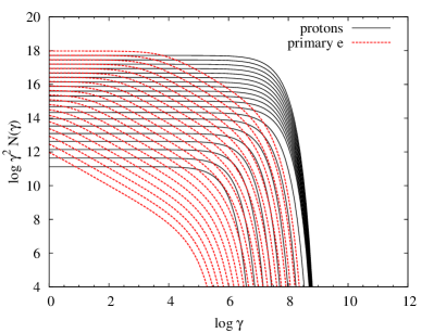
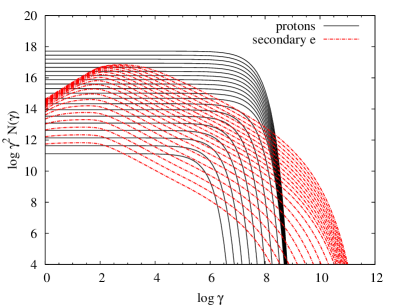
Figure 3: Snapshots of the particle distributions starting from $r=10^{{0.1}}r_{\rm in}$ and increasing by 0.25 in logarithmic units over its previous value up to a radius $r=10^{5}r_{\rm in}$. Left and right panels show the primary and secondary electron distributions (red) compared to the proton distribution (black). The accelerated proton and electron distributions at injection are modelled as $N_{\rm i}(\gamma)\propto\gamma^{-p}\exp(-\gamma/\gamma_{\rm i,M})$. The adopted parameters correspond to the default case described in text: $w=2$, $\alpha=0$, $a_{\rm ph}=0$, $s=2$, $\upsilon_{\rm w}=0.01c$, $\upsilon_{0}={0.03}c$, $r_{\rm in}=10^{13}$ cm   (i.e., $A_{\rm w}=10^{16}$ gr cm^-1), $L_{\rm SN}=10^{41}$ erg s^-1, $M_{\rm ej}={10}M_{\odot}$, $\epsilon_{\rm B}=0.01$, $\epsilon_{\rm p}=0.1$, $K_{\rm ep}=10^{-3}$, and $Q_{\rm 0p}=1$. All results can be linearly scaled for a realistic value of $Q_{\rm 0p}$.

In the general case of $s\neq 2$, the radial dependence of the total number of cooled and uncooled electrons can also be derived using basic scaling arguments, as we now detail. The number of primary electrons not affected by synchrotron cooling is $N_{\rm e}\propto\epsilon_{p}K_{\rm ep}\upsilon_{\rm s}^{2}r^{3-w}$, where the factor $r^{3-w}$ is related to the total accreted mass. As $\upsilon_{\rm s}\propto r^{\alpha}$ it follows that, quite generally, the number of uncooled primary electrons will be

$$N_{\rm e,<\gamma_{\rm c}}\propto r^{3-w+2\alpha}\gamma^{-s}$$ (74)

The number of primary electrons with $\gamma>\gamma_{\rm c}$ can then be simply written as

$$N_{\rm e,>\gamma_{\rm c}}=N_{\rm e,<\gamma_{\rm c}}\left(\gamma_{\rm c}\right)\left(\frac{\gamma}{\gamma_{\rm c}}\right)^{-s-1}.$$ (75)

Since $\gamma_{\rm c}\propto r^{w-\alpha-1}$ (see eq. (69)), we derive the scaling relation

$$N_{\rm e,>\gamma_{\rm c}}\propto r^{3-w+2\alpha}r^{w-\alpha-1}\gamma^{-s-1}\propto r^{2+\alpha}\gamma^{-s-1}.$$ (76)

Similar considerations apply to the case of secondary electrons. Their number is given by $N_{\rm p}t_{\rm dyn}/t_{\rm pp}$, or equivalently

$$N_{\rm e,<\gamma_{\rm c}}^{(\rm pp)}\propto r^{3-w+2\alpha}\gamma^{-s}r^{1-\alpha-w},$$ (77)

which results in the differential electron distribution

$$N_{\rm e,<\gamma_{\rm c}}^{(\rm pp)}\propto r^{4+\alpha-2w}\gamma^{-s}.$$ (78)

The distribution above the cooling break is then given by

$$N_{\rm e,>\gamma_{\rm c}}^{(\rm pp)}\propto r^{3-w}\gamma^{-s-1}.$$ (79)

4.1 An indicative example of particle evolution

An indicative example for the evolution of the particle distributions as obtained for the default case (see Table 1) is presented in Fig. 3. For clarity reasons, the primary and secondary electron distributions are displayed in the left and right panels with red dashed lines, respectively. For the adopted parameters, synchrotron radiation is the dominant cooling process for electrons (primary and secondary) for a wide range of shock radii, i.e. $r\approx 10^{14}-10^{17}$ cm, which corresponds to $t\approx{1.3-1300}$ days for $\upsilon_{0}={9\times 10^{3}}$ km s^-1. Here, the deceleration radius is $r_{\rm dec}\simeq 1$ pc.

At early times, the distribution of electrons is cooled due to synchrotron losses down to $\gamma\sim\gamma_{\rm e,m}$ with the cooling break (see eq. (69)) progressively moving to larger values as the magnetic field decreases; the cooling break is identified by the location where the slope in electron spectrum steepens from $-2$ to $-3$. On the contrary, the proton distribution at all radii has the same shape as at injection, since it is affected only by adiabatic losses. The proton maximum Lorentz factor at injection increases at early times according to eq. (31) (see the first three black curves from the bottom) and saturates at the value defined by eq. (23). The spacing between the curves shown in Fig. 3 reflects the radial (or, equivalently time) evolution of the different particle species. In particular, we find that $N_{\rm e}$ at a given Lorentz factor increases faster than $N_{\rm e}^{(\rm pp)}$, since the latter depends also on the CSM density profile that decreases with radius. In addition, the radial dependence of $N_{\rm i}$ as obtained numerically agrees quantitatively with the analytical predictions (see eqs. (70)-(73)).

Figure 4 shows with solid lines the evolution of the proton (black lines), primary electron (blue lines), secondary electron (red lines), magnetic (orange lines), and post-shock thermal ( cyan line) energy densities, for the same parameters as in Fig. 3. The ratios of the particle (magnetic) to thermal energy densities are overplotted with dashed lines. The ratio $U_{\rm B}/U_{\rm th}$, where $U_{\rm B}=B^{2}/8\pi$, is constant and equal to $\epsilon_{\rm B}$, as expected. Similarly, we find that $U_{\rm p}/U_{\rm th}\rightarrow 0.1\epsilon_{\rm p,-1}$, where $U_{\rm p}=(m_{\rm p}c^{2}/V)\int{\rm d}\gamma\,\gamma\,N_{\rm p}(\gamma)$ and $V\approx\pi r^{3}$ is the volume of the shocked shell. The early increase of the ratio $U_{\rm p}/U_{\rm th}$ is the result of the increasing proton maximum energy at small radii.

The ratio $U_{\rm e}/U_{\rm th}$ — where $U_{\rm e}$ is the primary electron energy density, defined in a similar way as $U_{\rm p}$ — increases, albeit with a slow rate. For all the considered radii, we find $U_{\rm e}/U_{\rm th}\ll 1$. This ratio is similar to the parameter $\epsilon_{\rm e}$ that is commonly used in the literature. However, it differs in essence, since $U_{\rm e}$ in our approach takes into account the cooling history of all electrons that have been injected at smaller radii. In the absence of cooling, $U_{\rm e}/U_{\rm p}\approx 10^{-3}K_{\rm ep,-3}I_{\rm e}/I_{\rm p}$, where $I_{\rm j}=\int_{\gamma_{\rm j,m}}^{\gamma_{\rm j,M}}{\rm d}\gamma\gamma^{-s+1}$. At large radii, where synchrotron cooling becomes less important, Fig. 4 shows indeed that $U_{\rm e}/U_{\rm p}\approx 10^{-3}$ (see solid black and blue lines). The increase of $U_{\rm e}/U_{\rm th}$ (blue dashed line) is another sign of less efficient electron cooling. Finally, the energy density of secondary electrons decreases faster compared to all other energy densities and its ratio to $U_{\rm th}$ is the lowest one at large radii.

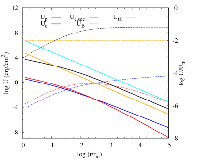
Figure 4: Evolution of the proton (black lines), primary electron (blue lines), secondary electron (red lines), magnetic (orange lines), and post-shock thermal ( cyan line) energy densities (solid lines), for the same parameters as in Fig. 3. The ratios of the particle (magnetic) to the thermal energy densities are overplotted with dashed lines of the corresponding color. All parameters are the same as in Fig. 3 except for $Q_{\rm 0p}$. Here, the exact value as obtained from eq. (18) was used.

5 Synchrotron emission

Having derived the evolution of the particle distributions as the forward shock propagates in the CSM, the synchrotron emission from both primary and secondary electrons, as well as from relativistic protons can be derived. Synchrotron emission at radio frequencies may be suppressed because of absorption processes, such as synchrotron self-absorption and free-free absorption. Moreover, in the presence of a background plasma, the synchrotron emission of a relativistic particle with Lorentz factor $\gamma$ will be suppressed at low enough frequencies, since the beaming of the radiation is not as strong at frequencies $\ll\gamma\omega_{\rm p}$ , where $\omega_{\rm p}$ is the plasma frequency; this is known as the Razin effect (Razin, 1960).

The intensity of synchrotron radiation at a given radius is given by

$$I_{\nu}=S_{\nu}(1-{\rm e}^{-\tau_{\nu}^{\rm ssa}})\rm{e}^{-\tau_{\nu}^{\rm ff}},$$ (80)

where $I_{\nu}$ is in units of erg cm^-2 s^-1 sr^-1 Hz^-1. In the above expression, $S_{\nu}=j_{\nu}/\alpha_{\nu}^{\rm ssa}$, $j_{\nu}$ is the synchrotron emissivity, $\alpha_{\nu}^{\rm ssa}$ is the synchrotron self-absorption coefficient (see e.g. eq. (6.50) in Rybicki & Lightman 1979), $\tau_{\nu}^{\rm ssa}=\alpha_{\nu}^{\rm ssa}h$ is the optical depth for synchrotron self-absorption, and $\tau_{\nu}^{\rm ff}\approx\alpha_{\nu}^{\rm ff}r$ is the optical depth for free-free absorption in the progenitor wind. Assuming that the ionized wind is composed of protons, $T_{\rm e}$ and $n_{\rm csm}$ are the temperature and number density of the unshocked wind, and $hv\ll kT_{\rm e}$, the free-free absorption coefficient can be written as (Rybicki & Lightman, 1986)

$$\alpha_{\nu}^{\rm ff}(r)=0.018T_{\rm e}^{-3/2}n_{\rm csm}^{2}(r)\bar{g}_{\rm ff}\nu^{-2},$$ (81)

where $\bar{g}_{\rm ff}\sim 1$ is the velocity averaged Gaunt factor for a Maxwellian distribution and $T_{\rm e}=10^{5}$ K is a typical value (see e.g. Fransson et al., 1996; Björnsson & Lundqvist, 2014). The luminosity per unit frequency is then given by

$$\frac{L_{\nu}}{4\pi}=4\pi r^{2}I_{\nu},$$ (82)

for $\nu\geq\nu_{\rm Rz}$, where $\nu_{\rm Rz}=2ecn_{\rm csm}(r)/B(r)\propto r^{-w/2-\alpha}$ is the Razin frequency (e.g. Rybicki & Lightman, 1986). At even lower frequencies the synchrotron emission essentially shuts down.

5.1 Characteristic frequencies

The typical synchrotron frequency of electrons with $\gamma=\gamma_{\rm c}$, which is defined as $\nu_{\rm c}=3eB\gamma_{\rm c}^{2}/4\pi m_{\rm e}c$, reduces to

$$\nu_{\rm c}\approx{0.03}\,\frac{(w-\alpha)^{2}}{(w-1)^{3/2}}\beta_{0,{-1.5}}^{1/2}\epsilon_{\rm B,-2}^{3/2}r_{\rm in,13}^{-1/2}\left(\frac{r}{r_{\rm in}}\right)^{3w/2-2-\alpha}\nobreak{\mathrm{\;GHz}},$$ (83)

for parameters relevant to this study. The Razin effect becomes important at frequencies below

$$\nu_{\rm Rz}\simeq 96\,\epsilon_{\rm B,-2}^{-1/2}\beta_{\rm 0,-1.5}^{-2}A_{\rm w,16}^{-1/2}\frac{r_{\rm in}}{r}\nobreak{\mathrm{\;GHz}},$$ (84)

where we used the default parameters listed in Table 1. For most parameters, we find that the Razin effect is not relevant for the radio emission, since $\nu_{\rm Rz}$ lies below the other characteristic absorption frequencies, which we calculate below. A characteristic free-free absorption frequency can also be defined by $\tau_{\rm ff}=1$. This is given by

$$\nu_{\rm ff}=0.134\,r^{1/2}T_{\rm e}^{-3/4}n_{\rm csm}(r),$$ (85)

which scales as $r^{-w+1/2}$. For $w=2$, the free-free absorption frequency reduces to

$$\nu_{\rm ff}\simeq{4\times 10^{5}}\,A_{\rm w,{16}}r_{\rm in,13}^{-3/2}T_{\rm e,5}^{-3/4}\left(\frac{r}{r_{\rm in}}\right)^{-3/2}\nobreak{\mathrm{\;GHz}}.$$ (86)

Typically, the synchrotron emission at $1-50$ GHz, where most radio observing facilities currently operate (e.g. JVLA, WSRT, GMRT etc.) will be free-free absorbed at early times, unless $A_{\rm w}\sim 10^{12}-10^{13}$ g cm^-1 (for a detailed analysis, see Murase et al., 2014).

Similarly, the synchrotron self-absorption frequency can be calculated through $\alpha_{\nu}^{\rm ssa}h=1$. In particular, an explicit solution of the synchrotron self-absorption frequency $\nu_{\rm ssa}$ can be derived using the $\delta$-function approximation for the single particle synchrotron emissivity and the expressions of $N_{\rm e}$ and $N_{\rm e}^{(\rm pp)}$ derived for $s=2$ and $\gamma\gtrless\gamma_{\rm c}$ (see Sect. 4). For typical parameter values, the electron distribution is expected to be cooled down to Lorentz factors close to the minimum one. For the sake of simplicity we, therefore, present the expression for $\nu_{\rm ssa}$ as obtained using eqs. (70) and (71), i.e. for the cooled electron distributions:

$$\nu_{\rm ssa}(r)=\nu_{0}X(r)K_{\rm ep}^{2/7}\epsilon_{\rm p}^{2/7}\epsilon_{\rm B}^{1/14}\beta_{0}^{9/14}r_{\rm in}^{-5/14}$$ (87)

where $X(r)$ is a function defined as

$$X(r)=\left(\frac{r}{r_{\rm in}}\right)^{-5w/14+\alpha}\left[1+\frac{3\times 10^{-3}(w-1)}{(4-w+2\alpha)K_{\rm ep}\beta_{0}^{2}}\left(\frac{r}{r_{\rm in}}\right)^{-w+1-\alpha}\right]^{2/7}$$ (88)

and $\nu_{0}$ is a numerical constant given by

$$\nu_{0}^{7/2}=\frac{45m_{\rm p}}{2^{10}m_{\rm e}\pi}\frac{\left(\pi\mu m_{\rm p}c^{4}\right)^{1/4}}{\ln\left(\frac{\gamma_{\rm p,M}}{\gamma_{\rm p,m}}\right)}\left(\frac{4(w-1)c^{2}}{\sigma_{T}}\right)^{5/4}\left(\frac{3m_{\rm e}c^{2}}{2hB_{\rm cr}}\right)^{1/2}$$ (89)

with $B_{\rm cr}=4.4\times 10^{13}$ G being the critical magnetic field strength. For the sake of simplicity, $\gamma_{\rm p,M}$ is treated as a constant with a typical value $10^{7}$. The second term in the parenthesis in eq. (88) corresponds to the secondary electrons, and is the dominant one at small radii, where the contribution of secondary synchrotron emission is expected to be more significant. For the default case (see Table 1), eq. (87) results in

$$\nu_{\rm ssa}(r)\simeq {2.5}\times 10^{3}\,\epsilon_{\rm B,-2}^{1/14}\epsilon_{\rm p,-1}^{2/7}K_{\rm ep,-3}^{2/7}\beta_{0,{-1.5}}^{-9/14}r_{\rm in,13}^{-5/14}\times$$

$$\left(\frac{r}{r_{\rm in}}\right)^{-5/7}\!\left[1+\frac{{1.5\times 10^{3}}}{K_{\rm ep,-3}\beta_{0,{-1.5}}^{2}}\left(\frac{r}{r_{\rm in}}\right)^{-1}\right]^{2/7}\nobreak{\mathrm{\;GHz}},$$

which is at least one order of magnitude lower than the free-free absorption frequency given by eq. (86). The peak synchrotron luminosity is thus expected at $\nu_{\rm ff}$, unless the density of the CSM is much lower than what is considered here; in this case, however, secondary electrons will not play a major role in the radio emission.

5.2 Synchrotron light curves

In this section we present analytical expressions for the power-law decay index of the optically thin synchrotron flux, using the $\delta$-function approximation for the single particle synchrotron emissivity. Starting from relations that apply to the cooled part of the electron distribution ($\gamma>\gamma_{\rm c}$) with $s=2$, we find the optically thin synchrotron luminosity at $\nu>\nu_{\rm c}$ to be

$$L_{\nu>\nu_{\rm c}}=\frac{1}{2}Q_{\rm 0e}m_{\rm e}c^{2}\upsilon_{0}\left(\frac{r}{r_{\rm in}}\right)^{2-w+3\alpha}\nu^{-1}$$ (91)

for shock- accelerated primary electrons, and

$$L_{\nu>\nu_{\rm c}}^{({\rm pp})}=\frac{1}{2}Q_{\rm 0e}^{(\rm pp)}m_{\rm e}c^{2}\upsilon_{0}\left(\frac{r}{r_{\rm in}}\right)^{3-2w+2\alpha}\nu^{-1}$$ (92)

for secondary electrons. At frequencies below the cooling break frequency ($\nu<\nu_{\rm c}$), the above expressions become

$$L_{\nu<\nu_{\rm c}}=\frac{Q_{\rm 0e}r_{\rm in}\sigma_{T}cB_{0}^{3/2}}{12\pi\left(4-w+2\alpha\right)}\left(\frac{hB_{\rm cr}}{m_{\rm e}c^{2}}\right)^{1/2}\left(\frac{r}{r_{\rm in}}\right)^{3-7w/4+7\alpha/2}\nu^{-1/2}$$ (93)

for shock-accelerated primary electrons, and

$$L_{\nu<\nu_{\rm c}}^{({\rm pp})}=\frac{Q_{\rm 0e}^{(\rm pp)}r_{\rm in}\sigma_{T}cB_{0}^{3/2}}{12\pi\left(5-2w+\alpha\right)}\left(\frac{hB_{\rm cr}}{m_{\rm e}c^{2}}\right)^{1/2}\left(\frac{r}{r_{\rm in}}\right)^{4-11w/4+5\alpha/2}\nu^{-1/2}$$ (94)

for secondary electrons. For the derivation of the above, we made use of eqs. (72) and (73). Moreover, eq. (92) and eq. (94) are derived for the case where the evolution of the proton distribution is dictated by adiabatic losses, which holds for most shock radii (see discussion after eq. (55)).

The power-law index of the optically thin synchrotron light curves depends on the temporal evolution of the shock velocity and on the CSM density profile. Interestingly, for the default choice of $w=2$ and $\alpha=0$, the synchrotron flux due to accelerated electrons is expected to be constant or slightly decaying as $r^{-1/2}$ depending on whether $\nu>\nu_{\rm c}$ or $\nu<\nu_{\rm c}$, respectively. If the secondary synchrotron radiation dominates in the radio frequencies, the light curve will decay faster due to the decreasing injection rate. We also note that the radial dependences presented in eqs. (91)-(94) apply also to cases where the accelerated distributions have $s>2$.

A simple relation between the power-law decay exponents of the primary ($t^{-\chi_{1}}$) and secondary ($t^{-\chi_{2}}$) synchrotron light curves can be derived

$$\chi_{2} = \left\{\begin{array}[]{cc}2\chi_{1}+\frac{1+4\alpha}{1-\alpha},&\nu>\nu_{\rm c}\\ \\ \frac{11}{7}\chi_{1}+\frac{\frac{5}{7}+3\alpha}{1-\alpha},&\nu<\nu_{\rm c}\end{array}\right.$$ (97)

where we made use of eqs. (91) - (94) and the relation $t\propto r^{1-\alpha}$. The transition from primary-dominated to secondary-dominated synchrotron emission at a given frequency band will be associated with a change in the decay slope of the radio light curve. Interestingly, the change $\Delta\chi\equiv\chi_{2}-\chi_{1}$ is independent of the electron cooling regime, namely

$$\Delta\chi=\frac{w-1+\alpha}{1-\alpha}.$$ (98)

Thus, the predicted break in the light curve for a wind-type CSM and a constant shock velocity is $\Delta\chi=1$. This break should be observable as long as the synchrotron luminosities of primary and secondary electrons are comparable at the transition time. As we show next (see e.g. Fig. 6), this condition is satisfied at high frequencies ($>100$ GHz) and early times.

5.3 Synchrotron peak luminosity

We present next the expressions for the peak synchrotron luminosity, whenever $\nu_{\rm ff}$ is the peak frequency. Although these are not applicable in all cases, e.g. if $\nu_{\rm ssa}>\nu_{\rm ff}$, they can be used as a quick reference whenever the mass loading parameter that is inferred from the observations is $\gtrsim 10^{14}$ gr cm^-1.

The respective peak luminosities can be obtained by inserting $\nu_{\rm ff}$ in the expressions of Sect. 5.2. These are given by

$$L_{\rm pk,\nu_{\rm ff}>\nu_{\rm c}}\simeq{1.8\times 10^{22}}\frac{K_{\rm ep,-3}\epsilon_{\rm p,-1}\beta_{0,{-1.5}}^{3}T_{\rm e,5}^{3/4}r_{\rm in,13}^{3/2}}{\ln\left(\gamma_{\rm p,M,8}\right)}\left(\frac{r}{r_{\rm in}}\right)^{3/2+3\alpha}\!\!\frac{\nobreak{\mathrm{\;erg}}}{\nobreak{\mathrm{\;Hz\,s}}}$$ (99)

and

$$L_{\rm pk,\nu_{\rm ff}>\nu_{\rm c}}^{(\rm pp)}\simeq\frac{6\times 10^{25}(w-1)}{4-w+2\alpha}\frac{\epsilon_{\rm p,-1}\beta_{0,{-1.5}}T_{\rm e,5}^{3/4}r_{\rm in,13}^{3/2}}{\ln\left(\gamma_{\rm p,M,8}\right)}\left(\frac{r}{r_{\rm in}}\right)^{5/2-w+2\alpha}\!\!\!\!\!\frac{\nobreak{\mathrm{\;erg}}}{\nobreak{\mathrm{\;Hz\,s}}}.$$ (100)

If $\nu_{\rm ff}\leq\nu_{\rm c}$ similar expressions for the peak luminosity can be derived. These read

$$L_{\rm pk,\nu_{\rm ff}<\nu_{\rm c}} \simeq {8.2\times 10^{24}}\frac{K_{\rm ep,-3}\epsilon_{\rm p,-1}\epsilon_{\rm B,-2}^{3/4}\beta_{0,{-1.5}}^{9/4}r_{\rm in,13}^{3/2}T_{\rm e,5}^{3/8}}{\ln\left(\gamma_{\rm p,M,8}\right)}\times$$ (101)

$$\frac{(w-1)^{5/4}}{4-w+2\alpha}\left(\frac{r}{r_{\rm in}}\right)^{11/4-5w/4+7\alpha/2}\frac{\nobreak{\mathrm{\;erg}}}{\nobreak{\mathrm{\;Hz\,s}}}$$

and

$$L_{\rm pk,\nu_{\rm ff}<\nu_{\rm c}}^{({\rm pp})} \simeq {2.5}\times 10^{28}\frac{\epsilon_{\rm p,-1}\epsilon_{\rm B,-2}^{3/4}T_{\rm e,5}^{3/8}r_{\rm in,13}^{3/2}\beta_{0,{-1.5}}^{1/4}}{\ln\left(\gamma_{\rm p,M,8}\right)}\times$$ (102)

$$\frac{(w-1)^{9/4}}{5-2w+\alpha}\left(\frac{r}{r_{\rm in}}\right)^{15/4-9w/4+5\alpha/2}\frac{\nobreak{\mathrm{\;erg}}}{\nobreak{\mathrm{\;Hz\,s}}}.$$

A few things worth commenting follow:

• the radial dependence of the peak luminosity is different if the synchrotron emission is dominated by primary or secondary electrons. In particular, for the case of a CSM wind density profile and a constant shock velocity, we find $L_{\rm pk,\nu_{\rm ff}>\nu_{\rm c}}\propto r^{3/2}$ $\left(L_{\rm pk,\nu_{\rm ff}>\nu_{\rm c}}^{(\rm pp)}\propto r^{1/2}\right)$ and $L_{\rm pk,\nu_{\rm ff}<\nu_{\rm c}}\propto r^{1/4}$ $\left(L_{\rm pk,\nu_{\rm ff}<\nu_{\rm c}}^{(\rm pp)}\propto r^{-3/4}\right)$ for primary (secondary) electrons.

• at early times (small radii) observations of the peak luminosity may generally probe the cooled secondary electron distribution (see eq. (100)), while at larger radii the peak luminosity tracks the uncooled primary electron distribution (see eq. (101)).

• for the parameter values of interest in this study, the electron distributions are expected to be cooled due to synchrotron losses, at least at early times. Thus, a characteristic time $t_{\rm pk,eq}$ can be defined by $L_{\rm pk,\nu_{\rm ff}>\nu_{\rm c}}=L_{\rm pk,\nu_{\rm ff}>\nu_{\rm c}}^{(\rm pp)}$. This is written as

  $$\frac{t_{\rm pk,eq}}{t_{\rm bo}}\simeq\frac{1}{1-\alpha}\left(\frac{Q_{\rm 0e}^{(\rm pp)}}{Q_{\rm 0e}}\right)^{\frac{1-\alpha}{w-1+\alpha}}\!\!=\left[\frac{{3.2\times 10^{3}}(w-1)}{4-w+2\alpha}K_{\rm ep,-3}^{-1}\beta_{0,{-1.5}}^{-2}\right]^{\frac{1-\alpha}{w-1+\alpha}},$$ (103)

  where eqs. (99) and (100) were used. In the above, $t_{\rm bo}\approx r_{\rm in}/\upsilon_{0}$ is the time of the shock breakout as long as this happens in the CSM wind. Interestingly, $t_{\rm pk,eq}$ depends only on two parameters, namely $K_{\rm ep}$ and $\upsilon_{0}$. As the shock velocity at breakout can be inferred from observations (e.g. Waxman et al., 2007; Katz et al., 2010), the transition time from secondary to primary synchrotron emission, at $\nu_{\rm pk}$, depends solely on one microphysical parameter related to the acceleration process, namely $K_{\rm ep}$. For $w=2$ and $\alpha=0$, one finds

  $$\frac{t_{\rm pk,eq}}{t_{\rm bo}}\simeq{1.6\times 10^{3}}\,K_{\rm ep,-3}^{-1}\beta_{0,{-1.5}}^{-2}.$$ (104)

The peak synchrotron luminosity is therefore expected to be dominated by the radiation of secondary electrons for

$$t\leq t_{\rm pk,eq}\simeq{190}\,K_{\rm ep,-3}^{-1}A_{\rm w,16}/\beta^{2}_{0,{-1.5}}\nobreak{\mathrm{\;d}}.$$ (105)

If the peak frequency lies below the cooling break frequency, i.e. $\nu_{\rm ff}<\nu_{\rm c}$, then this characteristic time is obtained from eqs. (101) and (102), and has the same dependence on the shock velocity and $K_{\rm ep}$ (but a different coefficient).

At the transition time the peak frequency is expected at

$$\nu_{\rm pk,eq}\simeq{5.6}\,T_{\rm e,5}^{-3/4}A_{\rm w,{16}}^{-1/2}K_{\rm ep,-3}^{3/2}\beta_{0,{-1.5}}^{3/2}\nobreak{\mathrm{\;GHz}}$$ (106)

where we assumed that $\nu_{\rm ff}$ is the peak synchrotron frequency and made use of eq. (85) and eq. (104). The analytical estimates for $t_{\rm pk,eq}$ and $\nu_{\rm pk}$ are in agreement with the numerical results presented in the next section (see e.g. Fig. 5).

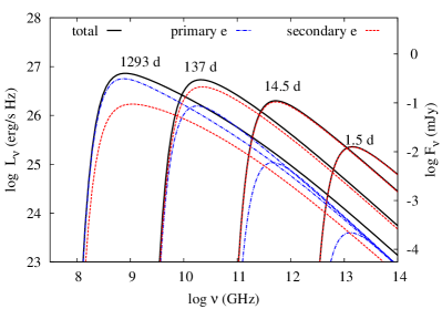
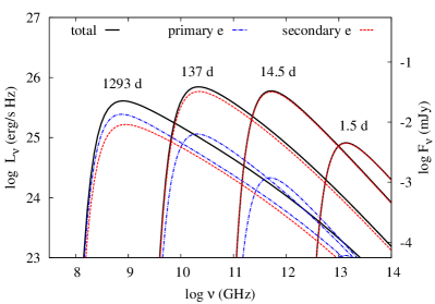
Figure 5: Snapshots of the synchrotron spectra (thick black lines) calculated for a wind-like CSM density profile ($w=2$) with mass loading parameter $A_{\rm w}=10^{16}$ g cm^-1 and a constant shock velocity $\upsilon_{0}={0.03}c$, after taking into account the Razin suppression, synchrotron self-absorption, and free-free absorption due to an electron plasma with temperature $T_{\rm e}=10^{5}$ K. Top and bottom panels are obtained for $\epsilon_{\rm B}=10^{-2}$ and $10^{-4}$, respectively. The contribution of the primary (blue dashed-dotted lines) and secondary (red dashed lines) electrons to the total synchrotron emission is also shown. The proton synchrotron contribution is negligible and for that reason not shown. For the flux conversion, a luminosity distance $d_{\rm L}=$ 40 Mpc was assumed. For the other parameters, see Table 1.

6 The effects of model parameters

In the following paragraphs we investigate the effect of the most important model parameters ($\epsilon_{\rm B},\alpha,\upsilon_{0}$, and $w$) on the radio spectra and light curves. Each case will be compared against the default one with parameters summarized in Table 1. The results that follow are numerically calculated based on the formalism presented in Sect. 3 and should be compared to the analytical expressions derived in the previous sections.

6.1 The role of $\epsilon_{\rm B}$

Figure 5 shows snapshots of the synchrotron spectra including the Razin suppression, synchrotron self-absorption, and free-free absorption, which is the dominant absorption process for the considered radii. Top and bottom panels are obtained for $\epsilon_{\rm B}=10^{-2}$ and $10^{-4}$, respectively. In both cases we find that at early times the synchrotron emission from the SN shock is dominated by the emission of secondaries electrons, whereas the opposite situation is realized at late times. For $\epsilon_{\rm B}=10^{-2}$ ( top panel), the spectral index of the optically thin synchrotron spectrum is $\beta=s/2=1$ ($L_{\nu}\propto\nu^{-\beta}$) at all radii, regardless whether the emission is dominated by primary or secondary electrons. The bottom panel of Fig. 5 illustrates the effect of a lower value of $\epsilon_{\rm B}$ on the synchrotron spectra. At early times, the magnetic field is still strong enough for the electrons to cool, thus leading to a spectral index $\beta=s/2=1$. At later times though, synchrotron cooling becomes less efficient and the synchrotron spectral index becomes $\beta=(s-1)/2=1/2$. The transition between the two cooling regimes is evident in the spectra of both primary and secondary electrons. In both cases, however, the spectral slope alone cannot be used to differentiate between primary and secondary synchrotron radiation, unless the shock-accelerated proton and electron distributions have different power-law slopes at injection. We note also that the peak luminosity in the right panel remains constant during the transition from secondary-dominated to primary-dominated synchrotron emission.

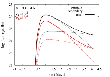
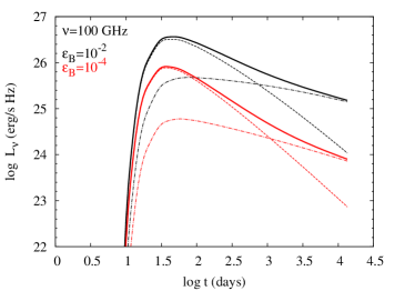
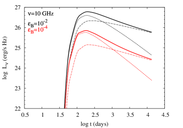
Figure 6: Radio light curves (thick solid lines) calculated at 1000 GHz, 100 GHz, and 10 GHz (from top to bottom) for the cases presented in Fig. 5. Black and red colored lines correspond to $\epsilon_{\rm B}=10^{-2}$ and $\epsilon_{\rm B}=10^{-4}$, respectively. Different types of lines show the contribution of primary and secondary electrons to the total synchrotron emission, as indicated in the legend. All other parameters used are listed in Table 1.

Table 2: Power-law decay index of the primary and secondary synchrotron light curves as determined numerically for $\alpha=0$ and two values of $\epsilon_{\rm B}$. All other parameters are the same as in Fig. 5 and Fig. 6. For reference, the analytically derived values for $\nu>\nu_{\rm c}$ ($\nu<\nu_{\rm c}$) are $\chi_{1}=0$ and $\chi_{2}=1$ ($\chi_{1}=0.5$, $\chi_{2}=1.5$).

	$10^{-2}$		$10^{-4}$
	$\chi_{1}$	$\chi_{2}$	$\chi_{1}$	$\chi_{2}$
1000	0.1	1.0	0.3	1.1
100	0.2	0.9	0.4	1.3
10	0.3	1.0	0.4	1.3

The radio light curves for the cases exemplified in Fig. 5 have been calculated at three characteristic frequencies (1000, 100 and 10 GHz) and presented in Fig. 6 (from top to bottom). The transition from secondary-dominated to primary-dominated synchrotron emission is demonstrated by a change in the decay slope of the light curve at 1000 GHz and 100 GHz. Moreover, the time of the transition does not depend on $\epsilon_{\rm B}$. All these features are in agreement with our analytical predictions in Sect. 5.2 and Sect. 5.3.

The power-law decay indices, whenever these can be defined, of the primary and secondary synchrotron fluxes are listed in Table 2. These should be compared to the analytical predictions for $\alpha=0$, namely $\chi_{1}=0$ and $\chi_{2}=1$ ($\chi_{1}=0.5$ and $\chi_{2}=1.5$, respectively) for $\nu>\nu_{\rm c}$ ($\nu<\nu_{\rm c}$, respectively). Indeed, for $\epsilon_{\rm B}=10^{-2}$ we find that the numerically derived indices are closer to the values given by eqs. (91) and (92), while $\chi_{1,2}$ approach the asymptotic values 0.5 and 1.5, respectively, for $\epsilon_{\rm B}=10^{-4}$. Small deviations from the analytical predictions are expected, since these are valid asymptotically, i.e. the distribution of electrons radiating at a given radio frequency should be described as $\gamma^{-s}$ or $\gamma^{-s-1}$.

6.2 The role of $A_{\rm w}$

To exemplify the role of the mass loading parameter we calculated the 10 GHz radio light curves for the default case of a wind-type CSM ($w=2$) and a constant shock velocity ($\alpha=0$). The results for $A_{\rm w}$ ranging between $10^{15}$ gr cm^-1 and $10^{17}$ gr cm^-1 are presented in Fig. 7. The light curves of the primary (dashed-dotted lines) and secondary (dashed lines) synchrotron emission at the chosen frequency are also shown. The calculations have been performed up to deceleration radius, which increases for lower values of $A_{\rm w}$ (see eq. (7)). Both the peak synchrotron luminosity and peak time increase for higher $A_{\rm w}$ values. The latter is the result of a higher free-free absorption frequency due to the denser CSM. This also leads to a higher magnetic field strength and a higher particle injection rate, which explains the increase of the peak luminosity. As $A_{\rm w}$ increases, the contribution of secondary electrons to the observed emission becomes larger, since the dependence of the secondary injection rate $Q_{\rm e}^{(\rm pp)}$ on the CSM density is stronger (see e.g. eqs. (18), (22) and (41)).

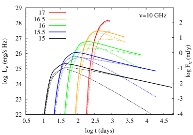
Figure 7: Radio light curves at 10 GHz for different values of the mass loading parameter $A_{\rm w}$. The (logarithmic) values (in g cm^-1 units) are listed in the inset legend. The contribution of primary and secondary synchrotron emission to the total one (thick solid lines) is shown as dashed-dotted and dashed lines, respectively. The results are plotted up to the deceleration time, which explains the abrupt interruption of the light curves. For the calculation of the radio flux, a source at a fiducial distance of 10 Mpc was adopted. All other parameters used are listed in Table 1. Here, the ejecta mass was assumed to be $5M_{\odot}$.

6.3 The role of $\upsilon_{0}$

The shock-breakout velocity $\upsilon_{0}$ may be indirectly inferred from the optical light curves (rise time and peak luminosity) of interaction-powered SNe (e.g. Ofek et al., 2014b). As typical values lie in the range $5\times 10^{3}-10^{4}$ km s^-1 (Ofek et al., 2014a), we have so far presented results for $\upsilon_{0}=0.03c$ ($9\times 10^{3}$ km s^-1). Here, we demonstrate the effects of the shock velocity at breakout on the radio light curves by adopting $\upsilon_{0}=0.1c$ ($3\times 10^{4}$ km s^-1). As illustrated in Fig. 8, higher shock velocities result in more luminous radio emission (see also eqs. (99)-(102)). This can be understood as an increase of the magnetic field strength and of the post-shock thermal energy density (see e.g. eq. (18)). Slower shocks, on the other hand, favour the production of secondary electrons, in agreement with the analytical predictions (Sect. 2.2). The transition time between secondary-dominated to primary-dominated synchrotron emission is strongly dependent on the shock velocity; for $\upsilon_{0}=0.1c$ the transition occurs at $\sim 10$ d, whereas secondaries dominate the 100 GHz radio emission until $10^{3}$ d for $\upsilon_{0}=0.03c$.

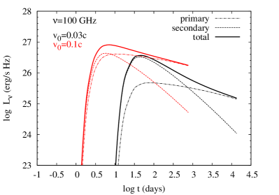
Figure 8: Radio light curves at 100 GHz for $\upsilon_{0}=9\times 10^{3}$ km s^-1 (black lines) and $\upsilon_{0}=3\times 10^{4}$ km s^-1. All other parameters are listed in Table 1.

6.4 The role of $T_{\rm e}$

The free-free absorption frequency is sensitive to the temperature of the upstream ionized CSM ($\nu_{\rm ff}\propto T^{-3/4}_{\rm e}$). This is exemplified in Fig. 9, where the 100 GHz and 10 GHz light curves are plotted for $T_{\rm e}=10^{5}$ (black, blue lines) and $10^{4}$ K (red, orange lines). A lower temperature shifts the peak time to later times, thus decreasing the time interval where the contribution of secondaries to the observed emission is significant. In particular, at 10 GHz the radio emission is expected to be dominated by the synchrotron emission of primary electrons at all times, unless $T_{\rm e}\gtrsim 10^{4}$ K (see blue and orange lines).

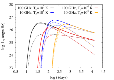
Figure 9: Radio light curves at 100 GHz and 10 GHz for two temperature values of the ionized unshocked CSM as indicated on the plot. All other parameters are listed in Table 1.

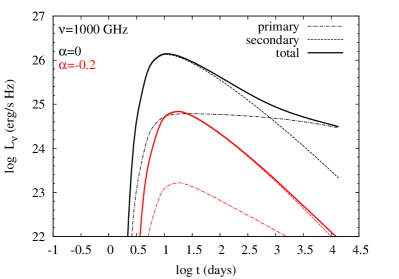
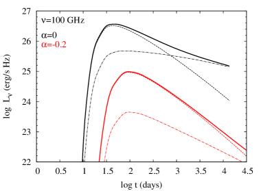
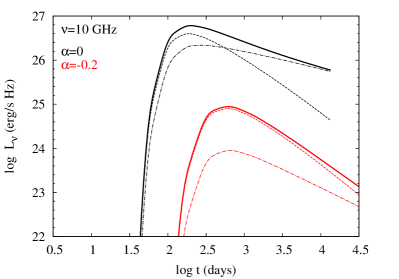
Figure 10: Radio light curves calculated at 1000 GHz, 100 GHz, and 10 GHz (from top to bottom) for a weakly decelerating SN shock with $\alpha=-0.2$ (red lines). In all panels, the results for the case of a constant shock velocity ($\alpha=0$) are plotted for comparison (black lines). Different types of lines show the contribution of primary and secondary electrons to the total synchrotron emission, as indicated in the legend. All other parameters used are listed in Table 1.

6.5 The role of $\alpha$

For specific combinations of the ejecta and CSM density profiles, a weakly decelerating SN shock ($\alpha\lesssim 0$) is a viable outcome (Chevalier, 1982; Berger et al., 2002; Soderberg et al., 2008, 2010; Chakraborti et al., 2015; Kamble et al., 2014c, 2015a; Fransson et al., 1996). The radio light curves at 10 GHz, 100 GHz and 1000 GHz for $\alpha=-0.2$ are presented in Fig. 10. In each panel, the respective light curves calculated for $\alpha=0$ are overplotted for a direct comparison. In both cases, the radio light curves of secondary synchrotron emission decay faster compared to those of primary synchrotron radiation. The total synchrotron luminosity is lower in the case of a weakly decelerating shock, since the injection rate of protons and, in turn, electrons decreases. It is also notable that in the case of $\alpha<0$, the secondary electrons contribute almost 100% to the total emission until late times, for observing frequencies as low as 10 GHz. At a given time, the weakly decelerating shock will be located at a smaller distance than that traveled by a shock moving with constant velocity, thus probing a dense CSM even at late times.

7 Relevance to SN radio observations

Several dozens of SNe within the local Universe (luminosity distance $d_{\rm L}<200\nobreak{\mathrm{\;Mpc}}$) have been detected in radio frequencies (see Chevalier & Fransson 2006 and Fig. 6 in Kamble et al. 2015a). All of these successful detections involve core-collapse SNe of all types with no detection of type Ia SN so far (see e.g. Chomiuk et al. (2015) and references therein).

The SN radio luminosity has a wide distribution arising primarily from the dispersion in progenitor mass-loss rates and SN shock velocities. The measured mass-loss rates of type Ibc SNe, which are related to compact massive Wolf-Rayet stars, are low ($\dot{M}_{\rm w}\sim 10^{-6}-10^{-5}\,{\rm M_{\odot}/yr}$) with typical wind velocities $\upsilon_{\rm w}=1000\,\nobreak{\mathrm{\;km\,s}}^{-1}$. With such low mass-loss rates these SN shocks cannot be powered by interaction with previously ejected matter from the progenitor. Thus, their wide range in luminosity could be attributed to the wide dispersion of their shock velocities. Indeed, the shocks in SNe Ibc are among the fastest ranging from $\beta\simeq 0.1-0.5$ (Kamble et al., 2014a).

Core collapse SNe due to their massive supergiant progenitors, such as type II SNe, are the best candidates for interaction-powered SNe. Progenitor mass-loss rates in SNe IIn can be as high as $\dot{M}_{\rm w}\sim 10^{-3}\,\nobreak{\mathrm{\;M_{\odot}/yr}}$, while their stellar winds are typically slow with $\upsilon_{\rm w}=10$ km s^-1). Radio observations of type IIn SNe show evidence of free-free absorption due to the optically thick ionized wind in the progenitor environment. As a result, the radio emission from these SNe rises slowly, with a typical rise time of $\sim 10^{3}$ days at $\sim$GHz frequencies.

A growing number of optically very luminous SNe with $L_{\rm bol}\geq 10^{43}\nobreak{\mathrm{\;ergs^{-1}}}$, which may be also powered by the CSM-shock interaction, is being detected by optical surveys (Smith et al., 2007; Gal-Yam et al., 2009; Quimby et al., 2011). Such an interaction scenario requires unprecedentedly high mass-loss rates for the SN progenitors, approaching $\dot{M}_{\rm w}\sim 1\,{\rm M_{\odot}/yr}$. Only a few attempts to observe the radio emission from SLSNe have been made without any detection so far (Chomiuk et al., 2011, 2012). Currently, it is not clear if there is a physical reason behind the absence of a radio signal or if it is an observational effect due to the large distances of SLSNe.

7.1 Synchrotron peak luminosity vs. peak time

It is instructive to view our results on the peak synchrotron luminosities of primaries and secondaries in the context of radio SNe observations. The peak luminosity versus peak time plot offers the most informative way to project the radio SNe (Chevalier, 1998; Chevalier & Fransson, 2006; Kamble et al., 2015b). The peak time $t_{\rm pk}$ corresponds to the time when the peak synchrotron frequency, namely $\nu_{\rm pk}\equiv\max(\nu_{\rm ff},\nu_{\rm ssa})$, crosses a fixed observing frequency ($\nu$). For the parameter values we are interested in, it is safe to assume that $\nu_{\rm pk}=\nu_{\rm ff}$. For the case of a wind-type CSM medium and a constant shock velocity, this happens at a shock radius

$$r_{\rm pk}\propto A_{\rm w}^{2/3}\nu^{-2/3}T_{\rm e}^{-1/2},$$ (107)

while the respective peak time is expressed as

$$t_{\rm pk}\propto A_{\rm w}^{{2/3}}\beta_{0}^{-1}\nu^{-2/3}T_{\rm e}^{-1/2}.$$ (108)

We remark that both the peak time and radius depend on $A_{\rm w}$: a denser CSM shifts $t_{\rm pk}$ to later times, having important consequences for the relative importance of secondary versus primary synchrotron emission. Moreover, the peak time is inversely proportional to the shock velocity, for a given mass loading parameter.

In the following, we assume that the electrons radiating at the peak synchrotron frequency belong to the cooled part of the distribution. The primary and secondary synchrotron luminosities at $\nu=\nu_{\rm pk}$ can be obtained by substitution of eqs. (107)-(108) into eqs. (99) and (100). Our results are summarized in Fig. 11 where the maximum of $L_{\rm pk,\nu_{\rm ff}>\nu_{\rm c}}$ (colored circles) and $L_{\rm pk,\nu_{\rm ff}>\nu_{\rm c}}^{(\rm pp)}$ (colored triangles) is plotted as a function of $t_{\rm pk}$. Measurements of radio SNe of various types (for details, see figure caption) are overplotted with filled and open black symbols. As most observations are performed at the $5$ GHz frequency band, the results shown in Fig. 11 are obtained for $\nu=5$ GHz. The two colored curves are obtained from the semi-analytical model for $\upsilon_{0}=0.1c$ and $0.03c$, as marked on the plot. The color coding corresponds to the value of the mass loading parameter $A_{\rm w}$ (see eq. (2)), as indicated in the color bar at the top. The black solid line is the locus of points with $L_{\rm pk,\nu_{\rm ff}>\nu_{\rm c}}=L_{\rm pk,\nu_{\rm ff}>\nu_{\rm c}}^{(\rm pp)}$. It divides the plot in two regions where the peak luminosity at $\nu_{\rm pk}=5$ GHz and $t_{\rm pk}$ is expected to be dominated by secondary (right to the line) or primary (left to the line) electrons. It is intriguing that the model-derived curve for $\beta_{0}=0.03c$ and $A_{\rm w}\gtrsim 10^{16}$ gr cm^-1 passes close to most of the type IIn observations (filled diamonds), suggesting that the peak synchrotron luminosity is dominated by the radiation of secondary electrons. Type IIn SNe could be therefore serve as candidate sources for the detection of hadronic acceleration in SN shocks.

Higher values of the mass loading parameter push the peak synchrotron luminosity (independently from the nature of radiating electrons) to higher values. As noted previously, the passage of $\nu_{\rm pk}$ across the 5 GHz frequency band happens at later times as $A_{\rm w}$ increases. Our results suggest that it is possible to probe the emission from secondaries with observations at 5 GHz if $t_{\rm pk}\simeq 300-1000$ days for shock velocities $\upsilon_{0}=0.03c-0.1c$ and dense CSM with $A_{\rm w}\gtrsim 10^{16}-10^{17}$ gr cm^-1.

The steep slope of the black solid line in Fig. 11 (that indicates the locus where $L_{\rm pk,\nu_{\rm ff}>\nu_{\rm c}}=L_{\rm pk,\nu_{\rm ff}>\nu_{\rm c}}^{(\rm pp)}$) implies a very strong dependence of the peak luminosity at the transition time $t_{\rm pk,eq}$ on $t_{\rm pk}$. Assuming that $\epsilon_{\rm p}$ and $T_{\rm e}$ are known parameters and using eqs. (5), (99), (86) and (104), it can be shown that

$$L_{\rm pk,eq}\propto t_{\rm pk,eq}^{6}\nu^{9}K_{\rm ep}^{-8}~{}~{}.$$ (109)

Interestingly, $L_{\rm pk,eq}$ depends only on a single parameter related to the acceleration process, that is $K_{\rm ep}$. The determination of the latter could be, therefore, possible if $L_{\rm pk,eq}$, $t_{\rm pk,eq}$ and $\nu$ were independently inferred from the observations. For example, a flattening of the light curve at $\nu=\nu_{\rm pk}$ by $\Delta\chi=1$ would denote $t_{\rm pk,eq}$, as illustrated in Figs. 6 and 10.

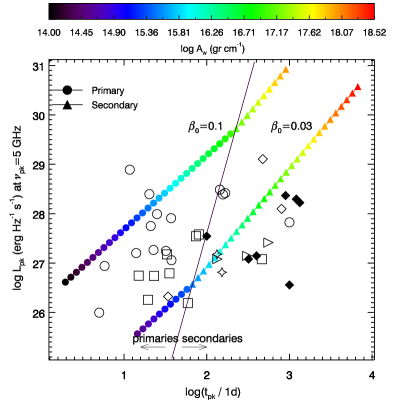
Figure 11: Peak spectral radio luminosity versus the peak time at a frequency $\nu=\nu_{\rm ff}=5$ GHz and two values of the shock velocity $\upsilon_{0}=0.1c$ and $0.03c$. The colored symbols correspond to the analytical predictions for cooled primary electrons (circles) and secondary electrons (triangles) given by eqs. (99) and (100), respectively. Only the maximum of $L_{\rm pk,\nu_{\rm ff}>\nu_{\rm c}}$ and $L_{\rm pk,\nu_{\rm ff}>\nu_{\rm c}}^{(\rm pp)}$ is shown. The black solid line is the locus of points with $L_{\rm pk,\nu_{\rm ff}>\nu_{\rm c}}=L_{\rm pk,\nu_{\rm ff}>\nu_{\rm c}}^{(\rm pp)}$. For the analytical calculations, we considered a wind-like CSM and a constant shock velocity. Color coding is used for the mass loading parameter $A_{\rm w}$, as indicated in the color bar at the top. Filled and open black symbols denote measurements from radio SNe of various types (data are from Kamble et al. 2015b): Ib/c, open circles; IIb, open squares; IIn, filled diamonds; IIL, open triangles; and II (SN 1978K, 1981K & 1982aa), open diamonds. Data for SN 1993J and 2013df are plotted as stars.

8 Discussion

We have presented a semi-analytical model for calculating the temporal evolution of primary and secondary particle distributions in the post-shock region of a SN forward shock propagating in a dense CSM. With the adopted formalism we were able to track the cooling history of all particles, which have been injected into the emission region up to a given radius, and to calculate the respective non-thermal radio emission. We have focused on the early phases of the SN evolution (i.e., before the Sedov phase) by presenting radio spectra and light curves for times prior to the deceleration time. The semi-analytical formalism can be, however, easily extended to the Sedov phase by adopting the adequate power-law index for the radial velocity profile. The light curves are expected to be steeper than those presented here, while at these later times, observations will probe the primary electron distribution.

So far, we have not discussed the origin of the magnetic field in the post-shock region of the SN shock. As the magnetic field of the unshocked progenitor wind is expected to be weak, magnetic field amplification is required for the particle acceleration. Non-resonant two-stream instabilities driven by cosmic-ray protons propagating ahead of the shock have been proposed as the amplification process (e.g. Bell & Lucek, 2001; Bell, 2004, 2005; Caprioli & Spitkovsky, 2014b; Cardillo et al., 2015). We caution, however, that if the large-scale magnetic field of the unshocked CSM is preferentially toroidal, the resulting shock will be quasi-perpendicular (i.e., with the magnetic field perpendicular to the shock normal), and particle acceleration will be inefficient. Thus, the relevant assumption is that the unshocked CSM field is weak or radial (e.g. Sironi et al., 2013; Caprioli & Spitkovsky, 2014a), which may be, however, questionable.

We have mostly focused on the case of a SN shock expanding in a smooth progenitor wind. However, our calculations are applicable to a generic CSM density profile. The environment of the progenitor star does not always have a smooth density profile. Density enhancements in the CSM may occur due to various reasons, such as variable stellar winds and interactions with the companion star, in case of a binary system. Interaction of the shock wave with such density enhancements would result in radio light curves exhibiting sudden and abrupt enhancements in (or dimming of) their brightness. Indeed, several radio SNe have been observed to show such features as early as a few weeks to as late as several months. Some examples of extreme variability include SN 1996cr (Bauer et al., 2008; Meunier et al., 2013), 2001em (Schinzel et al., 2009), 2003gk, 2004cc, 2004dk, 2004gq (Wellons et al., 2012), 2007bg (Salas et al., 2013), PTF11qcj (Corsi et al., 2014) and SN 2014C (Kamble et al., 2014b). Depending on the width and the mass of the intervening shell, the interaction of the shock wave with the shell could complicate the dynamics of the interaction (Chevalier & Liang, 1989; Dwarkadas, 2005, 2007; Chugai & Chevalier, 2006; Pan et al., 2013). Provided that the shock velocity can still be approximated as a power-law in radius and that the emission from the reverse shock is negligible, our formalism may still be employed to assess the radio synchrotron emission resulting from the interaction of the SN shock with a dense shell of uniform density.

Currently, the modelling of radio SNe involves the emission from primary electrons that are accelerated in the vicinity of the SN shock. We explicitly showed that secondary electrons may contribute significantly to the observed radio synchrotron emission, with their contribution becoming more important at higher radio frequencies (i.e. $\gtrsim 10-100$ GHz), for denser CSM (e.g. $A_{\rm w}\gtrsim 10^{16}$ gr cm^-1) and lower shock velocities (e.g. $\upsilon_{0}\lesssim 10^{4}$ km s^-1). As the radio brightness of the SN shock depends mainly on its radius and the number of radiating electrons, the inclusion of secondary electrons in the emission process could result in different estimates of the physical parameters, such as the mass-loss rate and/or the shock radius. The latter could be measured independently with high angular resolution imaging (e.g., Very Large Baseline Interferometry – VLBI) of nearby bright young SNe; this has been successfully carried out for about a dozen SNe and GRBs (Bietenholz, 2014; Pihlström et al., 2007; Taylor et al., 2004). Since the derived physical parameters from the synchrotron emission model depend on various microphysical parameters (e.g., $K_{\rm ep}$ and $\epsilon_{\rm p}$), independent radius measurements with VLBI observations could potentially constrain the synchrotron model (de Witt et al., 2016). Considering that the secondary electrons would contribute significantly at early times, a nearby bright and young SN will be a good candidate for direct assessment of this effect.

A robust prediction of our model is the flattening of the radio light curve by $\Delta\chi=(w-1+\alpha)/(1-\alpha)$ at high radio frequencies (i.e. $\gtrsim 10-100$ GHz) during the transition from secondary-dominated to primary-dominated synchrotron emission. Interestingly, $\Delta\chi$ is the same for all frequencies above or below the cooling break frequency. The change in the decay slope of the light curve is expected to be smooth (see e.g. left panels in Figs. 6 and 10). The transition time at the peak frequency should lie in the range $\sim 6-60$ d ($\sim$ 60$-$600 d, respectively) for $\upsilon_{0}=3\times 10^{4}$ km s^-1 ($\upsilon_{0}=9\times 10^{3}$ km s^-1, respectively) and $A_{\rm w}\sim 3\times 10^{15}-3\times 10^{16}$ gr cm^-1 (see also Fig. 7), while the peak frequency is, respectively, expected at $\sim 18-56$ GHz (3-10 GHz). However, it is not trivial to search for such breaks in existing radio data, especially if the shock is fast . The reason being that most of the radio observations are typically performed at 5-10 GHz, while some of the brightest SNe have been observed at higher frequencies, e.g. 40 GHz. The Atacama Large Millimeter Array (ALMA), with significant improvement in sensitivity in the millimeter waveband, would be an ideal telescope for the early detection of the SNe and the precise estimate of the secondary electron contribution to the SN brightness. ALMA would also be able to search for the predicted light curve flattening due to the rapid decline of the secondary electrons, thus providing a direct test of the model.

9 Summary

We have investigated the role of inelastic pp collisions as the SN shock sweeps through the dense CSM, focusing on the radio signatures from secondary electrons that are produced in the decay chain of charged pions. We have presented a semi-analytical one-zone model for calculating the temporal evolution of primary and secondary particle distributions in the post-shock region of the SN forward shock. With the adopted formalism, we were able to track the cooling history of all particles that have been injected into the emission region up to a given time, and calculated the radio spectra and light curves. These, upon comparison to the observations, can be used to constrain the acceleration efficiency of protons and electrons in fast supernova shocks.

We showed that, for a given SN shock expanding in a wind-like medium, secondary electrons control the early radio signatures, but their contribution decays faster than that of primary electrons, which dominate at later times. We derived the decay slope of radio light curves in the case of secondary-dominated ($t^{-\chi_{2}}$) and primary-dominated ($t^{-\chi_{1}}$) synchrotron emission and showed that, at a given frequency, a break of $\Delta\chi=\chi_{2}-\chi_{1}=(w-1+\alpha)/(1-\alpha)$ is expected during the transition between the two regimes. This simplifies to $\Delta\chi=1$ for the case of wind-type CSM and a constant shock velocity. The transition time at the peak frequency, in particular, was found to depend only on the mass-loading parameter for a wind-like CSM, the shock velocity $\upsilon_{0}$ and the ratio $K_{\rm ep}$ as $t\sim{190}\,K_{\rm ep,-3}^{-1}A_{\rm w,{16}}/\beta_{\rm 0,{-1.5}}^{2}$ d; the peak frequency at that time is expected at $\nu\sim{5.6}\,\nobreak{\mathrm{\;GHz}}\,T_{\rm e,5}^{-3/4}A_{\rm w,{16}}^{-1/2}K_{\rm ep,-3}^{3/2}\beta_{0,{-1.5}}^{3/2}$. Thus, radio observations performed at high frequencies $\sim{3-60}$ GHz and at times ${\sim 6-600}$ d may be used to probe the presence of secondary electrons for shocks with ${\upsilon_{0}=9\times 10^{3}-3\times 10^{4}}$ km s^-1 and dense CSM ($A_{\rm w}\sim 3\times 10^{15}-3\times 10^{16}$ gr cm^-1). Besides the transition time, the peak time of the light curve at a given observing frequency was also shown to be a strong predictor of the relative role of secondary versus primary electrons. We showed that early peak times imply a low-density CSM and a primary-dominated synchrotron emission. Late peak times (i.e., $t_{\rm pk}\gtrsim 250-1000$ d) at 5 GHz, on the contrary, suggest a fast ($\upsilon_{0}=9\times 10^{3}-3\times 10^{4}$ km s^-1) shock wave propagating in a dense medium ($A_{\rm w}\gtrsim 10^{16}-10^{17}$ gr cm^-1), where secondary electrons are likely to power the peak flux.

Appendix A Minimum momentum of accelerated particles

For typical velocities of early supernovae, $\upsilon_{\rm s}\sim 10^{4}\nobreak{\mathrm{\;km\,s}}^{-1}$, the thermal momentum of post-shock ions will be $p_{\rm th,p}\sim m_{\rm p}\upsilon_{\rm s}$, where factors of order unity are dropped. Thus, the bulk of the shocked ions will be non-relativistic. Recent hybrid and fully-kinetic simulations (e.g. Park et al., 2015) suggest that the power law of accelerated particles starts at $p_{\rm p,m}\sim 3p_{\rm th,p}$, namely the minimum momentum of the power-law distribution still falls in the non-relativistic regime. For a power-law distribution in momentum with power-law index $2<s<3$ extending from $p_{\rm p,m}$ up to ultra-relativistic energies most of the kinetic energy is carried by particles having $\gamma\sim 2$. On the contrary, for $s>3$, most of the energy is contributed by particles at $p_{\rm p,m}$. In fact, if $x=\gamma-1$, the particle distribution is $dN/dx\propto x^{-(s+1)/2}$ for $x\ll 1$ and the usual $dN/dx\propto x^{-s}$ for $x\gg 1$. Indeed, for $2<s<3$ the peak of $x^{2}dN/dx$, i.e., where most of the energy resides, occurs at $x\sim 1$, or equivalently $\gamma\sim 2$. Throughout the present study we assume that $2<s<3$. For a constant (or mildly decelerating) shock velocity, as expected in the free expansion phase, the injection momentum $p_{\rm p,m}$ does not change over time (or slightly decreases), which implies that the fraction of energy in non-relativistic – yet, non-thermal – protons, relative to the bulk of the particles, does not change (significantly) over time. Therefore, the assumption that a constant fraction of shock energy is channeled into non-thermal protons (either non-relativistic or relativistic) implies that a constant fraction of shock energy ($\epsilon_{\rm p}$, in our formalism) is channeled into ultra-relativistic protons.

Appendix B Bethe-Heitler energy loss timescale

Protons with Lorentz factors $\gamma_{\rm p,BH}\gtrsim m_{\rm e}c^{2}/\epsilon_{\rm ph}=5\times 10^{5}/(\epsilon_{\rm ph}/1\,{\rm eV})$ may lose energy through Bethe-Heitler pair production. Here, we derive the respective loss timescale, which may be recast in a similar form as $t_{\rm pp}$. The inverse of the Bethe-Heitler energy loss timescale is given by (Blumenthal, 1970)

$$t^{-1}_{\rm BH}(\gamma,r)=\frac{3}{8\pi\gamma}\sigma_{T}c\alpha_{\rm f}\frac{m_{\rm e}}{m_{\rm p}}\int_{2}^{\infty}\!\!d\kappa\ n_{\rm ph}\left(\frac{\kappa}{2\gamma}\right)\frac{\phi(\kappa)}{\kappa^{2}},$$ (110)

where $\alpha_{\rm f}$ is the fine structure constant, $n_{\rm ph}$ is the differential photon number density in the shocked shell, $\kappa=2\gamma\epsilon/m_{\rm e}c^{2}$, $\epsilon$ is the photon energy and $\phi(\kappa)$ is a function defined by a double integral (see eq. (3.12) in Chodorowski et al. (1992)). By approximating the photon field as $n_{\rm ph}(\epsilon)=(n_{\rm ph}/\epsilon_{\rm ph})\epsilon\delta(\epsilon-\epsilon_{\rm ph})$, where $n_{\rm ph}=U_{\rm ph}/\epsilon_{\rm ph}$, and by substitution in eq. (110) we find

$$t_{\rm BH}(\gamma,r)=\frac{4\pi m_{\rm p}}{3m_{\rm e}\alpha_{\rm f}}\frac{f^{-1}(x)}{c\sigma_{T}n_{\rm ph}(r)},$$ (111)

where $x\equiv 2\gamma\epsilon_{\rm ph}$ and $f(x)\equiv\phi(x)/x^{2}$ that has its maximum $f_{\max}\sim 1$ at $x\simeq 47$ (see Fig. 2 in Chodorowski et al. (1992)). Setting $f(x)\sim 1$, an effective cross section $\kappa_{\rm BH}\sigma_{\rm BH}\simeq 6\times 10^{-31}$ cm² can be defined and the timescale can be written as

$$t_{\rm BH}=\tau_{\rm BH}\left(\frac{r}{r_{\rm in}}\right)^{a_{\rm ph}+2},$$ (112)

where $\tau^{-1}_{\rm BH}=\kappa_{\rm BH}\sigma_{\rm BH}cU_{0}/\epsilon_{\rm ph}$ and eq. (27) was also used. By requiring $t_{\rm acc,p}=t_{\rm BH}$ and for $\gamma>\gamma_{\rm p,BH}$, a limiting Lorentz factor of the protons can be derived

$$\gamma_{\rm p,M}^{(3)}=\frac{eB_{0}\beta_{0}^{2}\epsilon_{\rm ph}}{6\kappa_{\rm BH}\sigma_{\rm BH}U_{0}m_{\rm p}c^{2}}\left(\frac{r}{r_{\rm in}}\right)^{2+a_{\rm ph}-a_{\rm B}+2\alpha},$$ (113)

which is similar to eq. (31).

Appendix C Asymptotic expressions for the primary and secondary electron distributions

Let us consider the following injection rate for primary electrons, with power-law energy slope $s=2$

$$Q_{\rm e}(\gamma,r)=\frac{Q_{\rm 0e}}{\gamma^{2}}\left(\frac{r_{\rm in}}{r}\right)^{w-2-2\alpha}H[\gamma-\gamma_{\rm e,m}]H[\gamma_{\rm e,M}(r)-\gamma]H[r-r_{\rm in}],$$ (114)

where $\gamma_{\rm e,M}(r)$ is obtained from $t_{\rm acc,e}=t_{\rm syn}$ (see eq. (23)) and the factor $r^{-w+2+2\alpha}$ accounts for a general CSM density profile and a radially dependent shock velocity (see eqs. (9) and (6), respectively). The evolution of an electron’s Lorentz factor is given by eq. (61), or equivalently

$$\gamma_{0}=\gamma\frac{r}{r_{0}}\left[1-\frac{K_{\rm syn}\gamma}{q_{\rm syn}}\left(\frac{r_{\rm in}}{r}\right)^{q_{\rm syn}-1}\left(\left(\frac{r}{r_{0}}\right)^{q_{\rm syn}}-1\right)\right]^{-1}.$$ (115)

where $q_{\rm syn}=2a_{\rm B}+\alpha=w-\alpha$. As we are interested in the synchrotron cooling dominated regime, the IC cooling term has dropped in the equation above. Using eq. (66) we find that the electron distribution is given by

$$N_{\rm e}(\gamma,r)=\frac{Q_{\rm 0e}}{\gamma^{2}}\frac{r_{\rm in}^{w-2-2\alpha}}{(4-w+2\alpha)r}\left(r^{4-w+2\alpha}-r_{\min}^{4-w+2\alpha}\right),$$ (116)

where $r_{\min}=\max(r_{\rm in},r_{\rm cr})$ and $r_{\rm cr}$ is defined by the condition $\gamma_{\rm e,M}(r_{0})-\gamma_{0}>0$. Using eq. (115) this condition leads to

$$1>\frac{\gamma}{\gamma_{\rm e,M}(r_{0})}\frac{r}{r_{0}}+\frac{K_{\rm syn}\gamma}{q_{\rm syn}}\left(\frac{r_{\rm in}}{r}\right)^{q_{\rm syn}-1}\left(\left(\frac{r}{r_{0}}\right)^{q_{\rm syn}}-1\right),$$ (117)

which should be solved with respect to $r_{0}$. The first term in the r.h.s. of the above relation contains information for the adiabatic cooling of electrons, whereas the second term is related to the synchrotron cooling. Since we are interested in deriving the evolution of the electron distribution when the dominant cooling process is synchrotron radiation, we can solve eq. (117) for $r_{0}$ after dropping the first term in the r.h.s. We find

$$r_{0}>r_{\rm cr}\equiv r\left(1+\frac{q_{\rm syn}}{K_{\rm syn}\gamma}\left(\frac{r}{r_{\rm in}}\right)^{q_{\rm syn}-1}\right)^{-\frac{1}{q_{\rm syn}}},$$ (118)

which can also be expressed as

$$\frac{r_{\rm cr}}{r}\approx\left\{\begin{array}[]{ll}1-\frac{1}{K_{\rm syn}\gamma}\left(\frac{r}{r_{\rm in}}\right)^{q_{\rm syn}-1},&\gamma\gg\gamma_{\rm br}\\ \\ \left[\frac{K_{\rm syn}\gamma}{q_{\rm syn}}\left(\frac{r}{r_{\rm in}}\right)^{q_{\rm syn}-1}\right]^{1/q_{\rm syn}},&\gamma\ll\gamma_{\rm br}\end{array}\right.$$ (122)

where

$$\gamma_{\rm c}\equiv\frac{q_{\rm syn}}{K_{\rm syn}}\left(\frac{r}{r_{\rm in}}\right)^{q_{\rm syn}-1}\propto r^{w-\alpha-1}.$$ (123)

We turn now to the lower integration limit $r_{\min}$, which is given by $r_{\min}\equiv\max[r_{\rm cr},r_{\rm in}]$. For $\gamma\gg\gamma_{\rm c}$ it can be shown that $r_{\min}=r_{\rm cr}$, whereas $r_{\min}=r_{\rm in}$ for $\gamma\ll\gamma_{\rm c}$. For most parameter values and at the early phases of the SN shock evolution, the radio emitting electrons belong to the cooled part of the spectrum ($\gamma>\gamma_{\rm c}$). For high values of $A_{\rm w}$, in particular, the electron distribution may cool due to synchrotron losses down to $\gamma\sim\gamma_{\rm e,m}$. Substitution of the high-$\gamma$ branch in eq. (122) to eq. (116) leads to

$$N_{\rm e}(\gamma,r)\approx\frac{Q_{\rm 0e}r_{\rm in}}{K_{\rm syn}\gamma^{3}}\left(\frac{r}{r_{\rm in}}\right)^{2+\alpha}.$$ (124)

Interestingly, the number of accelerated electrons with a given Lorentz factor does not dependent on the CSM density profile, e.g. $N_{\rm e}\propto\gamma^{-3}r^{2}$, for a constant shock velocity ($\alpha=0$). For $\gamma\ll\gamma_{\rm c}$, the electron distribution is simply given by eq. (116) with $r_{\min}=r_{\rm in}$. We remark that these results are valid as long as $\gamma_{\rm c}\gtrsim\gamma_{\rm e,m}$.

The above analysis can be directly applied to the secondary electrons, using the appropriate expression for the injection rate, which depends linearly on the distribution of relativistic protons (see e.g. eqs. (34) and (35)). The evolution of the proton distribution can be explicitly calculated for the generic injection profile of eq. (18), if it is dictated by the adiabatic losses (i.e., the catastrophic loss term in eq. (51) can be neglected). This is a good assumption, for all radii $r\gtrsim 10^{w+\alpha-1}\beta_{0,-1}^{-2(w+\alpha-1)}$ (see discussion after eq. (55)). In this case, the proton distribution is given by

$$N_{\rm p}(\gamma,r)=\frac{Q_{\rm 0p}r_{\rm in}\gamma^{-s}}{s-w+2\alpha+2}\left(\frac{r}{r_{\rm in}}\right)^{-w+3+2\alpha}\left[1-\left(\frac{r_{\rm in}}{r}\right)^{s-w+2+\alpha}\right],$$ (125)

where the term in the parenthesis is $\simeq 1$ for $r>r_{\rm in}$ and $s-w+2+\alpha>0$. Substitution of the above expression in eq. (36) results in

$$Q_{\rm e}^{(\rm pp)}(\gamma,r)=\frac{Q_{\rm 0e}^{(\rm pp)}}{\gamma^{s}}\left(\frac{r}{r_{\rm in}}\right)^{3-2w+\alpha}\!\!\!\!H[\gamma-\gamma_{\rm e,m}]H[\gamma_{\rm e,M}-\gamma]H[r-r_{\rm in}],$$ (126)

where the minimum and maximum Lorentz factors are now given by eq. (39). The electron distribution can be then explicitly derived for $s=2$. This is written as

$$N_{\rm e}^{(\rm pp)}(\gamma,r)=\frac{Q_{\rm 0e}^{(\rm pp)}}{\gamma^{2}}\frac{r_{\rm in}^{2w-3-\alpha}}{(5-2w+\alpha)r}\left(r^{5-2w+\alpha}-r_{\min}^{5-2w+\alpha}\right),$$ (127)

where $r_{\min}=\max(r,r_{\rm cr})$ and $r_{\rm cr}$ is same as in eq. (118). Making the the same approximations as before, the asymptotic expression for the secondary electron distribution in the synchrotron cooling dominated regime is

$$N_{\rm e}^{(\rm pp)}(\gamma,r)\approx\frac{Q_{\rm 0e}^{(\rm pp)}r_{\rm in}}{K_{\rm syn}\gamma^{3}}\left(\frac{r}{r_{\rm in}}\right)^{3-w}.$$ (128)

The synchrotron luminosity $L_{\nu}$ in the optically thin regime scales as $N_{\rm e}(r)B(r)^{(s^{\prime}+1)/2}$ (see e.g. Rybicki & Lightman, 1979), where $s^{\prime}=s+1$, if the emitting electrons belong to the cooled part of the distribution ($\gamma\gg\gamma_{\rm c}$) and $s^{\prime}=s$, otherwise. Using eq. (11) and eq. (124) for $s=2$ we find

$$L_{\nu}(r)\propto r^{2-w+3\alpha},\,{\rm or}$$ (129)

$$L_{\nu}(t)\propto t^{(2-w+3\alpha)/(1-\alpha)}.$$ (130)

If the luminosity at the particular frequency is dominated by secondary synchrotron emission, we find using eq. (11) and eq. (128) that

$$L^{(\rm pp)}_{\nu}(r)\propto r^{3-2w+2\alpha},\,{\rm or}$$ (131)

$$L^{(\rm pp)}_{\nu}(t)\propto t^{(3-2w+2\alpha)/(1-\alpha)}.$$ (132)

Appendix D Comparison of thermal and non-thermal energy densities

For certain SNe types that are characterized by a dense CSM, the shock breakout is expected to take place within the progenitor’s wind. After the shock breakout a collisionless shock may be formed, thus allowing the acceleration of particles (Katz et al., 2011; Murase et al., 2011). The X-ray photons produced at the shock soon after the shock breakout will be Compton down-scattered and thermalized, since $\tau_{\rm T}\sim c/\upsilon_{\rm s}=10-30$ at shock breakout (e.g. Chevalier & Irwin, 2011; Svirski et al., 2012). As long as $\tau_{\rm T}\gtrsim 1$, the energy density of thermal radiation may be written as (see e.g. Murase et al., 2014):

$$U_{\rm r,th}\simeq\tau_{\rm T}\frac{\xi_{\rm r}L_{\rm k}}{4\pi cr^{2}}\simeq\frac{c}{\upsilon_{0}}\frac{\xi_{\rm r}L_{\rm k}}{4\pi cr_{\rm in}^{2}}\left(\frac{r_{\rm in}}{r}\right)^{w+1},$$ (133)

where $\xi_{\rm r}$ is the fraction of the SN kinetic luminosity $L_{\rm k}$ that emerges as thermal radiation and $\tau_{\rm T}=(c/\upsilon_{0})\left(r_{\rm in}/r\right)^{w-1}$. Typical values of the thermal electron temperature in the shocked CSM are $T^{\rm(d)}_{\rm e}\sim 10^{8}-10^{9}$ K, although the exact values depend on whether thermal equilibrium between ions and electrons was achieved, or not (Fransson et al., 1996). If $T_{\rm e}^{\rm(d)}\gtrsim 2\times 10^{7}$ K, then thermal electrons cool via thermal bremsstrahlung, producing X-ray radiation. Hard ($\gtrsim 1-2$ keV) X-rays can escape without severe attenuation, if $\tau_{\rm T}\lesssim 1$. For a wind-like density profile ($w=2$), the energy density of X-ray photons is given by

$$U_{\rm X,ff}=\frac{L_{\rm ff}}{4\pi cr_{\rm in}^{2}}\left(\frac{r_{\rm in}}{r}\right)^{2},$$ (134)

where

$$L_{\rm ff}\simeq 1.5\times 10^{40}\,\frac{A_{\rm w,16}\left(T^{\rm(d)}_{\rm e,8}\right)^{1/2}}{\beta_{0,-1.5}}\frac{r_{\rm in}}{r}\nobreak{\mathrm{\;erg\,s}}^{-1},$$ (135)

where we used eq. (5.15b) by Rybicki & Lightman (1979), assuming an ionized CSM composed of pure hydrogen. It is interesting to compare $U_{\rm r,th}$ and $U_{\rm X,ff}$ with the non-thermal particle and magnetic energy densities in the downstream region of the SN forward shock. This is exemplified in Fig. 12 for $L_{\rm k}=10^{42}$ erg s^-1, $\xi_{\rm r}=0.1$ and $T_{\rm e}^{(d)}=10^{8}$ K. All other parameters are the same as in Fig. 4. At least for this indicative example, it is the magnetic energy density that dominates over $U_{\rm r,th}$ and $U_{\rm X,ff}$ at almost all radii. Thus, synchrotron cooling is expected to be the main energy loss process for electrons.

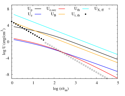
Figure 12: Same as in Fig. 4. In addition, $U_{\rm r,th}$ (filled symbols) and $U_{\rm X,ff}$ (open symbols) are shown for radii where $\tau_{\rm T}\geq 1$ and $<1$, respectively. Other parameter used are: $L_{\rm k}=10^{42}$ erg s^-1, $\xi_{\rm r}=0.1$ and $T_{\rm e}^{(d)}=10^{8}$ K.

Yet, the aforementioned radiation fields can, in principle, contribute to electron cooling via inverse Compton scattering. $U_{\rm r,th}$ turns out to be a more important source for electron cooling, since most of the inverse Compton scatterings between the electrons and X-ray bremsstrahlung photons take place in the Klein-Nishina regime. We note that these additional cooling channels for electrons were not taken into account in our calculations; we would have to rely on many assumptions regarding the thermal processes, which were not the focus of this study.

References

- Aartsen et al. (2015) Aartsen M. G. et al., 2015, Astrophysical Journal, 811, 52
- Aartsen et al. (2014a) Aartsen M. G. et al., 2014a, Physical Review Letters, 113, 101101
- Aartsen et al. (2014b) Aartsen M. G. et al., 2014b, Astrophysical Journal, 796, 109
- Axford et al. (1977) Axford W. I., Leer E., Skadron G., 1977, International Cosmic Ray Conference, 11, 132
- Barniol Duran (2014) Barniol Duran R., 2014, Monthly Notices of the Royal Astronomical Society, 442, 3147
- Barvainis et al. (1987) Barvainis R., McIntosh G., Predmore C. R., 1987, Nature, 329, 613
- Bauer et al. (2008) Bauer F. E., Dwarkadas V. V., Brandt W. N., Immler S., Smartt S., Bartel N., Bietenholz M. F., 2008, Astrophysical Journal, 688, 1210
- Bell (1978) Bell A. R., 1978, Monthly Notices of the Royal Astronomical Society, 182, 147
- Bell (2004) Bell A. R., 2004, Monthly Notices of the Royal Astronomical Society, 353, 550
- Bell (2005) Bell A. R., 2005, Monthly Notices of the Royal Astronomical Society, 358, 181
- Bell (2013) Bell A. R., 2013, Astroparticle Physics, 43, 56
- Bell & Lucek (2001) Bell A. R., Lucek S. G., 2001, Monthly Notices of the Royal Astronomical Society, 321, 433
- Berger et al. (2002) Berger E., Kulkarni S. R., Chevalier R. A., 2002, Astrophysical Journal Letters, 577, L5
- Bietenholz (2014) Bietenholz M. F., 2014, Publications of the Astronomical Society of Australia, 31, e002
- Björnsson & Fransson (2004) Björnsson C.-I., Fransson C., 2004, Astrophysical Journal, 605, 823
- Björnsson & Lundqvist (2014) Björnsson C.-I., Lundqvist P., 2014, Astrophysical Journal, 787, 143
- Blandford & Ostriker (1978) Blandford R. D., Ostriker J. P., 1978, Astrophysical Journal Letters, 221, L29
- Blasi (2013) Blasi P., 2013, Astronomy & Astrophysics Review, 21, 70
- Blumenthal (1970) Blumenthal G. R., 1970, Physical Review D, 1, 1596
- Blumenthal & Gould (1970) Blumenthal G. R., Gould R. J., 1970, Reviews of Modern Physics, 42, 237
- Caprioli & Spitkovsky (2014a) Caprioli D., Spitkovsky A., 2014a, Astrophysical Journal, 783, 91
- Caprioli & Spitkovsky (2014b) Caprioli D., Spitkovsky A., 2014b, Astrophysical Journal, 794, 46
- Cardillo et al. (2015) Cardillo M., Amato E., Blasi P., 2015, Astroparticle Physics, 69, 1
- Chakraborti et al. (2015) Chakraborti S. et al., 2015, Astrophysical Journal, 805, 187
- Chandra et al. (2012) Chandra P., Chevalier R. A., Chugai N., Fransson C., Irwin C. M., Soderberg A. M., Chakraborti S., Immler S., 2012, Astrophysical Journal, 755, 110
- Chevalier (1982) Chevalier R. A., 1982, Astrophysical Journal, 258, 790
- Chevalier (1998) Chevalier R. A., 1998, Astrophysical Journal, 499, 810
- Chevalier (2012) Chevalier R. A., 2012, Astrophysical Journal Letters, 752, L2
- Chevalier & Fransson (1994) Chevalier R. A., Fransson C., 1994, Astrophysical Journal, 420, 268
- Chevalier & Fransson (2003) Chevalier R. A., Fransson C., 2003, in Lecture Notes in Physics, Berlin Springer Verlag, Vol. 598, Supernovae and Gamma-Ray Bursters, Weiler K., ed., pp. 171–194
- Chevalier & Fransson (2006) Chevalier R. A., Fransson C., 2006, Astrophysical Journal, 651, 381
- Chevalier & Irwin (2011) Chevalier R. A., Irwin C. M., 2011, Astrophysical Journal Letters, 729, L6
- Chevalier & Li (2000) Chevalier R. A., Li Z.-Y., 2000, Astrophysical Journal, 536, 195
- Chevalier & Liang (1989) Chevalier R. A., Liang E. P., 1989, Astrophysical Journal, 344, 332
- Chodorowski et al. (1992) Chodorowski M. J., Zdziarski A. A., Sikora M., 1992, Astrophysical Journal, 400, 181
- Chomiuk et al. (2011) Chomiuk L. et al., 2011, Astrophysical Journal, 743, 114
- Chomiuk et al. (2012) Chomiuk L., Soderberg A., Margutti R., Berger E., Milisavljevic D., Sanders N., 2012, The Astronomer’s Telegram, 3931, 1
- Chomiuk et al. (2015) Chomiuk L. et al., 2015, ArXiv e-prints:1510.07662
- Chugai & Chevalier (2006) Chugai N. N., Chevalier R. A., 2006, Astrophysical Journal, 641, 1051
- Chugai & Danziger (1994) Chugai N. N., Danziger I. J., 1994, Monthly Notices of the Royal Astronomical Society, 268, 173
- Cohen & Ramaty (1973) Cohen J. M., Ramaty R., 1973, International Cosmic Ray Conference, 1, 634
- Corsi et al. (2014) Corsi A. et al., 2014, Astrophysical Journal, 782, 42
- Crowther (2007) Crowther P. A., 2007, Ann. Rev. Astron. Asrophys., 45, 177
- de Witt et al. (2016) de Witt A., Bietenholz M. F., Kamble A., Soderberg A. M., Brunthaler A., Zauderer B., Bartel N., Rupen M. P., 2016, Monthly Notices of the Royal Astronomical Society, 455, 511
- Dermer (1986) Dermer C. D., 1986, Astronomy & Astrophysics, 157, 223
- Dong et al. (2015) Dong S. et al., 2015, ArXiv e-prints:1507.03010
- Drout et al. (2013) Drout M. R. et al., 2013, Astrophysical Journal, 774, 58
- Dwarkadas (2005) Dwarkadas V. V., 2005, Astrophysical Journal, 630, 892
- Dwarkadas (2007) Dwarkadas V. V., 2007, Astrophysical Journal, 667, 226
- Finke & Dermer (2012) Finke J. D., Dermer C. D., 2012, Astrophysical Journal, 751, 65
- Fransson et al. (2014) Fransson C. et al., 2014, Astrophysical Journal, 797, 118
- Fransson et al. (1996) Fransson C., Lundqvist P., Chevalier R. A., 1996, Astrophysical Journal, 461, 993
- Gaisser (1990) Gaisser T. K., 1990, Cosmic rays and particle physics
- Gaisser et al. (1998) Gaisser T. K., Protheroe R. J., Stanev T., 1998, Astrophysical Journal, 492, 219
- Gal-Yam (2012) Gal-Yam A., 2012, Science, 337, 927
- Gal-Yam et al. (2009) Gal-Yam A. et al., 2009, Nature, 462, 624
- Giacinti & Bell (2015) Giacinti G., Bell A. R., 2015, Monthly Notices of the Royal Astronomical Society, 449, 3693
- Guo et al. (2014a) Guo X., Sironi L., Narayan R., 2014a, Astrophysical Journal, 794, 153
- Guo et al. (2014b) Guo X., Sironi L., Narayan R., 2014b, Astrophysical Journal, 797, 47
- IceCube Collaboration (2013) IceCube Collaboration, 2013, Science, 342
- Jones & Ellison (1991) Jones F. C., Ellison D. C., 1991, Space Science Reviews, 58, 259
- Kamble et al. (2015a) Kamble A. et al., 2015a, ArXiv e-prints:1504.07988
- Kamble et al. (2015b) Kamble A. et al., 2015b, ArXiv e-prints:1504.07988
- Kamble et al. (2014a) Kamble A., Soderberg A., Berger E., Zauderer A., Chakraborti S., Williams P., 2014a, ArXiv e-prints:1401.1221
- Kamble et al. (2014b) Kamble A., Soderberg A., Zauderer B. A., Chakraborti S., Margutti R., Milisavljevic D., 2014b, The Astronomer’s Telegram, 5763
- Kamble et al. (2014c) Kamble A. et al., 2014c, Astrophysical Journal, 797, 2
- Kasliwal et al. (2010) Kasliwal M. M. et al., 2010, Astrophysical Journal Letters, 723, L98
- Katz et al. (2010) Katz B., Budnik R., Waxman E., 2010, Astrophysical Journal, 716, 781
- Katz et al. (2011) Katz B., Sapir N., Waxman E., 2011, ArXiv e-prints:1106.1898
- Kelner et al. (2006) Kelner S. R., Aharonian F. A., Bugayov V. V., 2006, Physical Review D, 74, 034018
- Kiewe et al. (2012) Kiewe M. et al., 2012, Astrophysical Journal, 744, 10
- Kirk et al. (1998) Kirk J. G., Rieger F. M., Mastichiadis A., 1998, Astronomy & Astrophysics, 333, 452
- Klein & Chevalier (1978) Klein R. I., Chevalier R. A., 1978, Astrophysical Journal Letters, 223, L109
- Kopper et al. (2015) Kopper C., Giang W., Kurahashi N., 2015, To appear in the proceedings of The 34th International Cosmic Ray Conference PoS(ICRC2015)1081
- Mannheim & Schlickeiser (1994) Mannheim K., Schlickeiser R., 1994, Astronomy & Astrophysics, 286, 983
- Margutti et al. (2014) Margutti R. et al., 2014, Astrophysical Journal, 780, 21
- Margutti et al. (2013) Margutti R. et al., 2013, Astrophysical Journal, 778, 18
- Mastichiadis (1996) Mastichiadis A., 1996, Astronomy & Astrophysics, 305, L53
- Mastichiadis & Kirk (1995) Mastichiadis A., Kirk J. G., 1995, Astronomy & Astrophysics, 295, 613
- Matzner & McKee (1999) Matzner C. D., McKee C. F., 1999, Astrophysical Journal, 510, 379
- Mészáros (2006) Mészáros P., 2006, Reports on Progress in Physics, 69, 2259
- Metzger et al. (2016) Metzger B. D., Caprioli D., Vurm I., Beloborodov A. M., Bartos I., Vlasov A., 2016, Monthly Notices of the Royal Astronomical Society, 457, 1786
- Meunier et al. (2013) Meunier C. et al., 2013, Monthly Notices of the Royal Astronomical Society, 431, 2453
- Moderski et al. (2005) Moderski R., Sikora M., Coppi P. S., Aharonian F., 2005, Monthly Notices of the Royal Astronomical Society, 363, 954
- Morlino & Caprioli (2012) Morlino G., Caprioli D., 2012, Astronomy & Astrophysics, 538, A81
- Murase et al. (2011) Murase K., Thompson T. A., Lacki B. C., Beacom J. F., 2011, Physical Review D, 84, 043003
- Murase et al. (2014) Murase K., Thompson T. A., Ofek E. O., 2014, Monthly Notices of the Royal Astronomical Society, 440, 2528
- Nakar & Sari (2010) Nakar E., Sari R., 2010, Astrophysical Journal, 725, 904
- Ofek et al. (2014a) Ofek E. O. et al., 2014a, Astrophysical Journal, 788, 154
- Ofek et al. (2014b) Ofek E. O. et al., 2014b, Astrophysical Journal, 781, 42
- Padovani & Resconi (2014) Padovani P., Resconi E., 2014, Monthly Notices of the Royal Astronomical Society, 443, 474
- Pan et al. (2013) Pan T., Patnaude D., Loeb A., 2013, Monthly Notices of the Royal Astronomical Society, 433, 838
- Park et al. (2015) Park J., Caprioli D., Spitkovsky A., 2015, Physical Review Letters, 114, 085003
- Petropoulou & Mastichiadis (2009) Petropoulou M., Mastichiadis A., 2009, Astronomy & Astrophysics, 507, 599
- Picozza et al. (2013) Picozza P. et al., 2013, Journal of Physics Conference Series, 409, 012003
- Pihlström et al. (2007) Pihlström Y. M., Taylor G. B., Granot J., Doeleman S., 2007, Astrophysical Journal, 664, 411
- Piran (2004) Piran T., 2004, Reviews of Modern Physics, 76, 1143
- Protheroe & Clay (2004) Protheroe R. J., Clay R. W., 2004, Publications of the Astronomical Society of Australia, 21, 1
- Quimby et al. (2011) Quimby R. M. et al., 2011, Nature, 474, 487
- Quimby et al. (2013) Quimby R. M., Yuan F., Akerlof C., Wheeler J. C., 2013, Monthly Notices of the Royal Astronomical Society, 431, 912
- Rabinak & Waxman (2011) Rabinak I., Waxman E., 2011, Astrophysical Journal, 728, 63
- Razin (1960) Razin V. A., 1960, Izuestiya Vys. Ucheb. Zaued. Radiofiz., 3, 921
- Rieger et al. (2007) Rieger F. M., Bosch-Ramon V., Duffy P., 2007, Astrophysics and Space Science, 309, 119
- Rybicki & Lightman (1979) Rybicki G. B., Lightman A. P., 1979, Radiative processes in astrophysics
- Rybicki & Lightman (1986) Rybicki G. B., Lightman A. P., 1986, Radiative Processes in Astrophysics
- Salas et al. (2013) Salas P., Bauer F. E., Stockdale C., Prieto J. L., 2013, Monthly Notices of the Royal Astronomical Society, 428, 1207
- Santana et al. (2014) Santana R., Barniol Duran R., Kumar P., 2014, Astrophysical Journal, 785, 29
- Schinzel et al. (2009) Schinzel F. K., Taylor G. B., Stockdale C. J., Granot J., Ramirez-Ruiz E., 2009, Astrophysical Journal, 691, 1380
- Schlickeiser (2002) Schlickeiser R., 2002, Cosmic Ray Astrophysics
- Sironi et al. (2013) Sironi L., Spitkovsky A., Arons J., 2013, Astrophysical Journal, 771, 54
- Smith et al. (2007) Smith N. et al., 2007, Astrophysical Journal, 666, 1116
- Soderberg et al. (2008) Soderberg A. M. et al., 2008, Nature, 453, 469
- Soderberg et al. (2010) Soderberg A. M. et al., 2010, Nature, 463, 513
- Soderberg et al. (2005) Soderberg A. M., Kulkarni S. R., Berger E., Chevalier R. A., Frail D. A., Fox D. B., Walker R. C., 2005, Astrophysical Journal, 621, 908
- Stawarz et al. (2008) Stawarz Ł., Ostorero L., Begelman M. C., Moderski R., Kataoka J., Wagner S., 2008, Astrophysical Journal, 680, 911
- Sturner et al. (1997) Sturner S. J., Skibo J. G., Dermer C. D., Mattox J. R., 1997, Astrophysical Journal, 490, 619
- Svirski et al. (2012) Svirski G., Nakar E., Sari R., 2012, Astrophysical Journal, 759, 108
- Tammi & Duffy (2009) Tammi J., Duffy P., 2009, Monthly Notices of the Royal Astronomical Society, 393, 1063
- Tan et al. (2001) Tan J. C., Matzner C. D., McKee C. F., 2001, Astrophysical Journal, 551, 946
- Taylor et al. (2004) Taylor G. B., Frail D. A., Berger E., Kulkarni S. R., 2004, Astrophysical Journal Letters, 609, L1
- Truelove & McKee (1999) Truelove J. K., McKee C. F., 1999, Astrophysical Journal Suppl. Ser., 120, 299
- Völk et al. (2005) Völk H. J., Berezhko E. G., Ksenofontov L. T., 2005, Astronomy & Astrophysics, 433, 229
- Waxman & Loeb (2001) Waxman E., Loeb A., 2001, Physical Review Letters, 87, 071101
- Waxman et al. (2007) Waxman E., Mészáros P., Campana S., 2007, Astrophysical Journal, 667, 351
- Weaver (1976) Weaver T. A., 1976, Astrophysical Journal Suppl. Ser., 32, 233
- Webb et al. (1984) Webb G. M., Drury L. O., Biermann P., 1984, Astronomy & Astrophysics, 137, 185
- Wellons et al. (2012) Wellons S., Soderberg A. M., Chevalier R. A., 2012, Astrophysical Journal, 752, 17
- Yuan et al. (2012) Yuan Q., Liu S., Bi X., 2012, Astrophysical Journal, 761, 133
- Zhang et al. (2015) Zhang B.-B., van Eerten H., Burrows D. N., Ryan G. S., Evans P. A., Racusin J. L., Troja E., MacFadyen A., 2015, Astrophysical Journal, 806, 15
- Zirakashvili & Ptuskin (2015) Zirakashvili V. N., Ptuskin V. S., 2015, ArXiv e-prints:1510.08387