Frequency-hiding Dependency-preserving Encryption for Outsourced Databases

Abstract

The cloud paradigm enables users to outsource their data to computationally powerful third-party service providers for data management. Many data management tasks rely on the data dependencies in the outsourced data. This raises an important issue of how the data owner can protect the sensitive information in the outsourced data while preserving the data dependencies. In this paper, we consider functional dependency ($FD$), an important type of data dependency. We design a $FD$-preserving encryption scheme, named $F^{2}$, that enables the service provider to discover the $FDs$ from the encrypted dataset. We consider the frequency analysis attack, and show that the $F^{2}$ encryption scheme can defend against the attack under Kerckhoff’s principle with provable guarantee. Our empirical study demonstrates the efficiency and effectiveness of $F^{2}$.

1 Introduction

With the fast growing of data volume, the sheer size of today’s data sets is increasingly crossing the petabyte barrier, which far exceeds the capacity of an average business computer. In-house solutions may be expensive due to the purchase of software, hardware, and staffing cost of in-house resources to administer the software. Lately, due to the advent of cloud computing and its model for IT services based on the Internet and big data centers, a new model has emerged to give companies a cheaper alternative to in-house solutions: the users outsource their data management needs to a third-party service provider. Outsourcing of data and computing services is becoming commonplace and essential.

Many outsourced data management applications rely on data dependencies in the outsourced datasets. A typical type of data dependency is functional dependency (FD). Informally, a $FD:A\rightarrow B$ constraint indicates that an attribute set $A$ uniquely determines an attribute set $B$. For example, the FD Zipcode$\rightarrow$City indicates that all tuples of the same Zipcode values always have the same City values. FDs serve a wide range of data applications, for example, improving schema quality through normalization [3, 6], and improving data quality in data cleaning [10]. Therefore, to support these applications in the outsourcing paradigm, it is vital that FDs are well preserved in the outsourced datasets.

ID A B C $t_{1}$ $a_{1}$ $b_{1}$ $c_{1}$ $t_{2}$ $a_{1}$ $b_{1}$ $c_{2}$ $t_{3}$ $a_{1}$ $b_{1}$ $c_{3}$ $t_{4}$ $a_{1}$ $b_{1}$ $c_{1}$	ID A B C $t_{1}$ $\hat{a}_{1}$ $\hat{b}_{1}$ $\hat{c}_{1}$ $t_{2}$ $\hat{a}_{1}$ $\hat{b}_{1}$ $\hat{c}_{2}$ $t_{3}$ $\hat{a}_{1}$ $\hat{b}_{1}$ $\hat{c}_{3}$ $t_{4}$ $\hat{a}_{1}$ $\hat{b}_{1}$ $\hat{c}_{1}$
(a) Base table $D$	(b) $\hat{D}_{1}$ encrypted
($FD:A\rightarrow B$)	by deterministic encryption
	(not frequency-hiding)
ID A B C $t_{1}$ $\hat{a}_{1}^{1}$ $\hat{b}_{1}^{1}$ $\hat{c}_{1}^{1}$ $t_{2}$ $\hat{a}_{1}^{1}$ $\hat{b}_{1}^{2}$ $\hat{c}_{2}^{1}$ $t_{3}$ $\hat{a}_{1}^{2}$ $\hat{b}_{1}^{1}$ $\hat{c}_{3}^{1}$ $t_{4}$ $\hat{a}_{1}^{2}$ $\hat{b}_{1}^{2}$ $\hat{c}_{1}^{2}$	ID A B C $t_{1}$ $\hat{a}_{1}^{1}$ $\hat{b}_{1}^{1}$ $\hat{c}_{1}^{1}$ $t_{2}$ $\hat{a}_{1}^{1}$ $\hat{b}_{1}^{1}$ $\hat{c}_{2}^{1}$ $t_{3}$ $\hat{a}_{1}^{2}$ $\hat{b}_{1}^{2}$ $\hat{c}_{3}^{1}$ $t_{4}$ $\hat{a}_{1}^{2}$ $\hat{b}_{1}^{2}$ $\hat{c}_{1}^{2}$
(c) $\hat{D}_{2}$ encrypted by	(d) $\hat{D}_{3}$ encrypted by
probabilistic encryption on	probabilistic encryption
$A$ and $B$ individually	on attribute set $\{A,B\}$
(not FD-preserving)	(Frequency-hiding & FD-preserving)

Figure 1: An example of various encryption schemes

Outsourcing data to a potentially untrusted third-party service provider (server) raises several security issues. One of the issues is to protect the sensitive information in the outsourced data. The data confidentiality problem is traditionally addressed by means of encryption [8]. Our goal is to design efficient FD-preserving data encryption methods, so that the FDs in the original dataset still hold in the encrypted dataset. A naive method is to apply a simple deterministic encryption scheme (i.e. the same plaintext values are always encrypted as the same ciphertext for a given key) on the attributes with FDs. For instance, consider the base table $D$ in Figure 1 (a). Assume it has a FD: $F$: $A\rightarrow B$. Figure 1 (b) shows the encrypted dataset $\hat{D}_{1}$ by applying a deterministic encryption scheme on individual values of the attributes in $D$. Apparently $F$ is preserved in $\hat{D}_{1}$. However, this naive method has drawbacks. One of the main drawbacks is that the deterministic encryption scheme is vulnerable against the frequency analysis attack, as the encryption preserves the frequency distribution. The attacker can easily map the ciphertext (e.g., $\hat{a}_{1}$) to the plaintext values (e.g., $a_{1}$) based on their frequency.

A straightforward solution to defend against the frequency analysis attack is instead of the deterministic encryption schemes, using the probabilistic encryption schemes (i.e., the same plaintext values are encrypted as different ciphertexts) to hide frequency. Though the probabilistic encryption can provide provable guarantee of semantic security [11], it may destroy the FDs in the data. As an example, consider the table $D$ shown in Figure 1 (a) again. Figure 1 (c) shows an instance $\hat{D}_{2}$ by applying the probabilistic encryption scheme at the attributes $A$, $B$, and $C$ individually. We use the notation $\hat{a}_{i}^{j}$ ($\hat{b}_{i}^{j}$, $\hat{c}_{i}^{j}$, resp.) as a ciphertext value of $a_{i}$ ($b_{i}$, $c_{i}$, resp.) by the probabilistic encryption scheme. The four occurrences of the plaintext value $a_{1}$ are encrypted as two $\hat{a}_{1}^{1}$s (tuple $t_{1}$ and $t_{2}$) and two $\hat{a}_{1}^{2}$s (tuple $t_{3}$ and $t_{4}$), while the four occurrences of the plaintext value $b_{1}$ are encrypted as two $\hat{b}_{1}^{1}$s (tuple $t_{1}$ and $t_{3}$) and two $\hat{b}_{1}^{2}$s (tuple $t_{2}$ and $t_{4}$). Now the frequency distribution of the plaintext and ciphertext values is not close. However, the FD $A\rightarrow B$ does not hold on $\hat{D}_{2}$ anymore, as the same (encrypted) value $\hat{a}_{1}$ of attribute $A$ is not associated with the same cipher value of attribute $B$. This example shows that the probabilistic encryption scheme, if it is applied on individual attributes, cannot preserve the FDs. This raises the challenge of finding the appropriate attribute set to be encrypted by the probabilistic encryption scheme. It is true that applying the probabilistic encryption scheme on FD attributes as a unit (e.g., on {A, B} as shown in Figure 1 (d)) can preserve FDs. However, finding $FDs$ needs intensive computational efforts [16]. The data owner may lack of computational resources and/or knowledge to discover FDs by herself. Therefore, we assume that FDs are not available for the encryption.

Contributions. In this paper, we design $F^{2}$, a frequency-hiding, FD-preserving encryption scheme based on probabilistic encryption. We consider the attacker who may possess the frequency distribution of the original dataset as well as the details of the encryption scheme as the adversary knowledge. We make the following contributions.

(i) $F^{2}$ allows the data owner to encrypt the data without awareness of any FD in the original dataset. To defend against the frequency analysis attack on the encrypted data, we apply the probabilistic encryption in a way that the frequency distribution of the ciphertext values is always flattened regardless of the original frequency distribution. This makes $F^{2}$ robust against the frequency analysis attack. To preserve FDs, we discover maximal attribute sets ($MASs$) on which $FDs$ potentially exist. Finding $MASs$ is much cheaper than finding $FDs$, which enables the data owner to afford its computational cost. The probabilistic encryption is applied at the granularity of $MAS$s.

(ii) We consider both cases of one single $MAS$ and multiple $MASs$, and design efficient encryption algorithms for each case. The challenge is that when there are multiple $MASs$, there may exist conflicts if the encryption is applied on each $MAS$ independently. We provide conflict resolution solution, and show that the incurred amounts of overhead by conflict resolution is bounded by the size of the dataset as well as the number of overlapping $MAS$ pairs.

(iii) Applying probabilistic encryption may introduce false positive FDs that do not exist in the original dataset but in the encrypted data. We eliminate such false positive FDs by adding a small amount of artificial records. We prove that the number of such artificial records is independent of the size of the outsourced dataset.

(iv) We formally define the frequency analysis attack, and the $\alpha$-security model to defend against the frequency analysis attack. We show that $F^{2}$ can provide provable security guarantee against the frequency analysis attack, even under the Kerckhoffs’s principle [27] (i.e., the encryption scheme is secure even if everything about the encryption scheme, except the key, is public knowledge).

(v) We evaluate the performance of $F^{2}$ on both real and synthetic datasets. The experiment results show that $F^{2}$ can encrypt large datasets efficiently with high security guarantee. For instance, it takes around 1,500 seconds to encrypt a benchmark dataset of size 1GB with high security guarantee. Furthermore, $F^{2}$ is much faster than FD discovery. For instance, it takes around 1,700 seconds to discover FDs from a dataset of 64KB records, while only 8 seconds to encrypt the dataset by $F^{2}$.

Applications This is the first algorithm that preserves useful FDs with provable security guarantees against the frequency analysis attack in the outsourcing paradigm. To see the relevance of this achievement, consider that FDs have been identified as a key component of several classes of database applications, including data schema refinement and normalization [3, 6, 21], data cleaning [4, 10], and schema-mapping and data exchange [20]. Therefore, we believe that the proposed FD-preserving algorithm represents a significant contribution towards the goal of reaching the full maturity of data outsourcing systems (e.g., database-as-a-service [13] and data-cleaning-as-a-service [9] systems).

The rest of this paper is organized as follows. Section 2 describes the preliminaries. Section 3 discusses the details of our encryption scheme. Section 4 presents the security analysis. Section 5 evaluates the performance of our approach. Related work is introduced in Section 6, and Section 7 concludes the paper.

2 Preliminaries

2.1 Outsourcing Setting

We consider the outsourcing framework that contains two parties: the data owner and the service provider (server). The data owner has a private relational table $D$ that consists of $m$ attributes and $n$ records. We use $r[X]$ to specify the value of record $r$ on the attribute(s) $X$. To protect the private information in $D$, the data owner encrypts $D$ to $\hat{D}$, and sends $\hat{D}$ to the server. The server discovers the dependency constraints of $\hat{D}$. These constraints can be utilized for data cleaning [10] or data schema refinement [3]. In principle, database encryption may be performed at various levels of granularity. However, the encryption at the coarse levels such as attribute and record levels may disable the dependency discovery at the server side. Therefore, in this paper, we consider encryption at cell level (i.e., each data cell is encrypted individually). Given the high complexity of FD discovery [16], we assume that the data owner is not aware of any FD in $D$ before she encrypts $D$.

2.2 Functional Dependency

In this paper, we consider functional dependency (FD) as the data dependency that the server aims to discover. Formally, given a relation $R$, there is a FD between a set of attributes $X$ and $Y$ in $R$ (denoted as $X\rightarrow Y$) if for any pair of records $r_{1},r_{2}$ in $R$, if $r_{1}[X]=r_{2}[X]$, then $r_{1}[Y]=r_{2}[Y]$. We use $LHS(F)$ ($RHS(F)$, resp.) to denote the attributes at the left-hand (right-hand, resp.) side of the FD $F$. For any FD $F:X\rightarrow Y$ such that $Y\subseteq X$, $F$ is considered as trivial. In this paper, we only consider non-trivial $FDs$. It is well known that for any FD $F:X\rightarrow Y$ such that $Y$ contains more than one attribute, $F$ can be decomposed to multiple functional dependency rules, each having a single attribute at the right-hand side. Therefore, for the following discussions, WLOG, we assume that the FD rules only contain one single attribute at the right-hand side.

2.3 Deterministic and Probabilistic Encryption

Our encryption scheme $\Pi$ consists of the following three algorithms:

• $k\leftarrow KeyGen(\lambda)$ generates a key based on the input security parameter $\lambda$.

• $y\leftarrow Encrypt(x,k)$ encrypts the input value $x$ using key $k$ and outputs the ciphertext $y$.

• $x\leftarrow Decrypt(y,k)$ computes the plaintext $x$ based on the ciphertext $y$ and key $k$.

Based on the relationship between plaintexts and ciphertexts, there are two types of encryption schemes: deterministic and probabilistic schemes. Given the same key and plaintext, a deterministic encryption scheme always generates the same ciphertext. One weakness of the deterministic ciphertexts is that it is vulnerable against the frequency analysis attack. On the other hand, the probabilistic encryption scheme produces different ciphertexts when encrypting the same message multiple times. The randomness brought by the probabilistic encryption scheme is essential to defend against the frequency analysis attack [18]. In this paper, we design a FD-preserving, frequency-hiding encryption scheme based on probabilistic encryption. We use the private probabilistic encryption scheme based on pseudorandom functions [17]. Specifically, for any plaintext value $p$, its ciphertext $e=<r,F_{k}(r)\oplus p>$, where $r$ is a random string of length $\lambda$, $F$ is a pseudorandom function, $k$ is the key, and $\oplus$ is the XOR operation.

2.4 Attacks and Security Model

In this paper, we consider the curious-but-honest server, i,e., it follows the outsourcing protocols honestly (i.e., no cheating on storage and computational results), but it is curious to extract additional information from the received dataset. Since the server is potentially untrusted, the data owner sends the encrypted data to the server. The data owner considers the true identity of every cipher value as the sensitive information which should be protected.

Frequency analysis attack. We consider that the attacker may possess the frequency distribution knowledge of data values in $D$. In reality, the attacker may possess approximate knowledge of the value frequency in $D$. However, in order to make the analysis robust, we adopt the conservative assumption that the attacker knows the exact frequency of every plain value in $D$, and tries to break the encryption scheme by utilizing such frequency knowledge. We formally define the following security game $Exp_{\mathcal{A},\Pi}^{freq}$ on the encryption scheme $\Pi=(KeyGen,Encrypt,Decrypt)$ :

• A random key $k$ is generated by running $KeyGen$. A set of plaintexts $\mathcal{P}$ is encrypted by running $Encrypt(\mathcal{P},k)$. A set of ciphertext values $\mathcal{E}\leftarrow Encrypt(\mathcal{P},k)$ is returned.

• A ciphertext value $e$ is randomly chosen from $\mathcal{E}$. Let $p=Decrypt(e,k)$. Let $freq_{\mathcal{P}}(p)$ and $freq_{\mathcal{E}}(e)$ be the frequency of $p$ and $e$ respectively. Let $freq(\mathcal{P})$ be the frequency distribution of $\mathcal{P}$. Then $e$, $freq_{\mathcal{E}}(e)$ and $freq(\mathcal{P})$ is given to the adversary $\mathcal{A}^{freq}$.

• $\mathcal{A}^{freq}$ outputs a value $p^{\prime}\in\mathcal{P}$.

• The output of the experiment is defined to be $1$ if $p^{\prime}=Decrypt(e,k)$, and $0$ otherwise. We write $Exp_{\mathcal{A},\Pi}^{freq}=1$ if the output is $1$ and in this case we say that $\mathcal{A}^{freq}$ succeed.

Security Model. To measure the robustness of the encryption scheme against the frequency analysis attack, we formally define $\alpha$-security.

Definition 2.1

[$\alpha$-security] An encryption scheme $\Pi$ is $\alpha$-secure against frequency analysis attack if for every adversary $\mathcal{A}^{freq}$ it holds that

$$Pr[Exp_{\mathcal{A},\Pi}^{freq}=1]\leq\alpha,$$

where $\alpha$ is a value between $0$ and $1$.

Intuitively, the smaller $\alpha$ is, the stronger security that $\Pi$ is against the frequency analysis attack. In this paper, we aim at designing an encryption scheme that provides $\alpha$-security for any given $\alpha\in(0,1)$.

Kerckhoffs’s principle. Kerckhoffs’s principle [27] requires that a cryptographic system should be secure even if everything about the system, except the key, is public knowledge. Thus, we also require the encryption scheme to satisfy $\alpha$-security under Kerckhoffs’s principle (i.e., the adversary knows the details of $F^{2}$ encryption algorithm).

3 FD-preserving Encryption

The key to design a FD-preserving encryption algorithm is to first identify the set of attributes on which the probabilistic encryption scheme is applied. We have the following theorem to show that for any FD $F$, if the probabilistic encryption scheme is applied on the attribute set that includes both $LHS(F)$ and $RHS(F)$, $F$ is still preserved in the encrypted data.

Theorem 3.1

Given a dataset $D$ and any FD $F$ of $D$, let the attribute set $\mathcal{A}$ be the attribute sets on which the probabilistic encryption scheme is applied on, and let $\hat{D}$ be the encryption result. Then $F$ always holds in $\hat{D}$ if $LHS(F)\cup RHS(F)\subseteq\mathcal{A}$.

Proof 3.2.

Assume that there is a FD: $A\rightarrow B$ which holds in $D$ but not in $\hat{D}$. It must be true that there exists at least one pair of records $r_{1}$, $r_{2}$ such that $r_{1}[A]=r_{2}[A]$ and $r_{1}[B]=r_{2}[B]$ in $D$, while in $\hat{D}$, $\hat{r_{1}}[A]=\hat{r_{2}}[A]$ but $\hat{r_{1}}[B]\neq\hat{r_{2}}[B]$. According to the HS scheme which is applied on an attribute set $\cal{A}$ s.t. $LHS(F)\cup RHS(F)\subseteq\cal{A}$, there are two cases. First, if $r_{1}$ and $r_{2}$ are taken as the same instance, then $\hat{r_{1}}$ and $\hat{r_{2}}$ have the same value in every attribute. It cannot happen as $\hat{r_{1}}[B]\neq\hat{r_{2}}[B]$. Second, if $r_{1}$ and $r_{2}$ are taken as different instances, then it must be true that $\hat{r_{1}}[A]\neq\hat{r_{2}}[A]$ and $\hat{r_{1}}[B]\neq\hat{r_{2}}[B]$ according to Requirement 2 of the HS scheme. So $\hat{r_{1}}$ and $\hat{r_{2}}$ cannot break the FD: $A\rightarrow B$ in $\hat{D}$.

To continue our running example, consider the base table in Figure 1 (a). Figure 1 (d) shows an example table $\hat{D}_{3}$ of applying the probabilistic encryption scheme on the attribute set $\{A,B\}$. By this scheme, the four instances of $(a_{1},b_{1})$ are encrypted as $(\hat{a}_{1}^{1},\hat{b}_{1}^{1}$) and $(\hat{a}_{1}^{2},\hat{b}_{1}^{2}$). Now the FD $A\rightarrow B$ still holds on $\hat{D}_{3}$.

Based on Theorem 3.1, we formally define our FD-preserving probabilistic encryption scheme. We use $|\sigma_{\mathcal{A}=r[\mathcal{A}]}(D)|$ to specify the number of records in $D$ that have the same value as $r[\mathcal{A}]$, for a specific record $r$ and a set of attributes $\mathcal{A}$.

Definition 3.1

[FD-preserving probabilistic encryption scheme] Given a table $D$, a FD $F$ of $D$, and a set of attributes $\mathcal{A}=\{A_{1},\dots,A_{g}\}$ of $D$ such that $LHS(F)\cup RHS(F)\subseteq\mathcal{A}$, for any instance $r\{a_{1},\dots,a_{g}\}\in D$, let $f=|\sigma_{\mathcal{A}=r[\mathcal{A}]}(D)|$. When $f>1$, the FD-preserving probabilistic encryption scheme encrypts the $f$ instances as $t>1$ unique instances $\{r_{1},\dots,r_{t}\}$, such that $r_{1}=\{\hat{a}_{1}^{1},\dots,\hat{a}_{g}^{1}\}$ of frequency $f_{1}$, $\dots$, and $r_{t}=\{\hat{a}_{1}^{t},\dots,\hat{a}_{g}^{t}\}$ of frequency $f_{t}$. We require that:

• Requirement 1: $\sum_{i=1}^{t}f_{i}=f$;

• Requirement 2: $\forall i\ (1\leq i\leq g)$, $\hat{a}_{i}^{x}\neq\hat{a}_{i}^{y}$, for all $x,y\in[1,t]$ where $x\neq y$.

Requirement 1 requires when encrypting a plaintext value set to multiple different ciphertext instances, the sum of frequency of these ciphertext instances is the same as the frequency of the plaintext value set. Requirement 2 requires that the ciphertext values of the same plaintext value set do not overlap at any single attribute. The aim of Requirement 2 is to provide $\alpha$-security under Kerckhoffs’s principle (more details in Section 4.2). We require that $f>1$, since the probabilistic encryption scheme becomes a deterministic encryption scheme when $f=1$.

Our FD-preserving probabilistic encryption method consists of four steps: (1) finding maximum attribute sets; (2) splitting-and-scaling; (3) conflict resolution; and (4) eliminating false positive FDs. We explain the details of these four steps in the following subsections.

3.1 Step 1: Finding Maximum Attribute Sets

Theorem 3.1 states that the set of attributes on which the probabilistic encryption scheme is applied should contain all attributes in FDs. Apparently the set of all attributes of $D$ satisfies the requirement. However, it is not a good solution since it is highly likely that there does not exist a probabilistic encryption scheme, due to the reason that $f=|\sigma_{\mathcal{A}=r[\mathcal{A}]}(D)|$ is more likely to be 1 when $\mathcal{A}$ contains more attributes. Now the main challenge is to decide the appropriate attribute set $\mathcal{A}$ that the probabilistic encryption scheme will be applied on, assuming that the data owner is not aware of the existence of any $FD$. To address this challenge, we define the maximum attribute set on which there exists at least one instance whose frequency is greater than 1. Formally,

Definition 3.2

[Maximum Attribute Set ($MAS$)] Given a dataset $D$, an attribute set $\mathcal{A}$ of $D$ is a maximum attribute set $MAS$ if: (1) there exists at least an instance $\mathcal{a}$ of $\mathcal{A}$ such that $|\sigma_{\mathcal{A}=\mathcal{a}}(D)|>1$; and (2) for any attribute set $A^{\prime}$ of $D$ such that $\mathcal{A}\subseteq\mathcal{A}^{\prime}$, there does not exist an instance $\mathcal{a}^{\prime}$ of $\mathcal{A}^{\prime}$ s.t. $|\sigma_{\mathcal{A}^{\prime}=\mathcal{a}^{\prime}}(D)|>1$.

Our goal is to design the algorithm that finds all $MASs$ of a given dataset $D$. Note that the problem of finding $MASs$ is not equivalent to finding FDs. For instance, consider the base table $D$ in Figure 1 (a). Its $MASs$ is {A, B, C}. But its FD is $A\rightarrow B$. In general, given a set of $MAS$s $\cal M$ and a set of FDs $\cal F$, for each FD $F\in\cal F$, there always exists at least an $MAS$ $M\in\cal M$ such that $(LHS(F)\cup RHS(F))\subseteq M$.

In general, finding $MASs$ is quite challenging given the exponential number of attribute combinations to check. We found out that our $MAS$ is equivalent to the maximal non-unique column combination [15]. Informally, maximal non-unique column combination refers to a set of columns whose projection has duplicates. It has been shown that finding all (non-)unique column combination is an NP-hard problem [12]. In [15], the authors designed a novel algorithm named $Ducc$ that can discover maximal non-unique column combinations efficiently. The complexity of $Ducc$ is decided by the solution set size but not the number of attributes. Therefore, we adapt the $Ducc$ algorithm [15] to find $MASs$. Due to the space limit, we omit the details of the algorithm here. For each discovered $MAS$, we find its partitions [16]. We say two tuples $r$ and $r^{\prime}$ are equivalent with respect to a set of attributes $X$ if $r[X]=r^{\prime}[X]$.

Definition 3.3

[Equivalence Class ($EC$) and Partitions] [16] The equivalence class ($EC$) of a tuple $r$ with respect to an attribute set $X$, denoted as $r_{X}$, is defined as $r_{X}=\{r^{\prime}|r[A]=r^{\prime}[A],\forall A\in X\}$. The size of $r_{X}$ is defined as the number of tuples in $r_{X}$, and the representative value of $r_{X}$ is defined as $r[X]$. The set $\pi_{X}=\{r_{X}|r\in D\}$ is defined as a partition of $D$ under the attribute set $X$. That is, $\pi_{X}$ is a collection of disjoint sets ($ECs$) of tuples, such that each set has a unique representative value of a set of attributes $X$, and the union of the sets equals $D$.

As an example, consider the dataset $\hat{D}_{3}$ in Figure 1 (d), $\pi_{\{A,B\}}$ consists of two $EC$s whose representative values are $\{\hat{a}_{1}^{1},\hat{b}_{1}^{1}\}$ and $\{\hat{a}_{1}^{2},\hat{b}_{1}^{2}\}$. Apparently, a $MAS$ is an attribute set whose partitions contain at least one equivalence class whose size is more than 1.

3.2 Step 2: Splitting-and-scaling Encryption

After the $MASs$ and their partitions are discovered, we design two steps to apply the probabilistic encryption scheme on the partitions: (1) grouping of $ECs$, and (2) splitting and scaling on the $EC$ groups. Next, we explain the details of the two steps.

3.2.1 Step 2.1. Grouping of Equivalence Classes

To provide $\alpha$-security, we group the $EC$s in the way that each equivalence class belongs to one single group, and each group contains at least $k\geq[\frac{1}{\alpha}]$ $EC$s, where $\alpha$ is the threshold for $\alpha$-security. We use $ECG$ for the equivalence class group in short.

We have two requirements for the construction of $ECGs$. First, we prefer to put $EC$s of close sizes into the same group, so that we can minimize the number of new tuples added by the next splitting & scaling step (Section 3.2.2). Second, we do not allow any two $EC$s in the same $ECG$ to have the same value on any attribute of $MAS$. Formally,

Definition 3.4

[Collision of $ECs$] Given a $MAS$ $M$ and two equivalence classes $C_{i}$ and $C_{j}$ of $M$, we say $C_{i}$ and $C_{j}$ have collision if there exists at least one attribute $A\in M$ such that $C_{i}[A]=C_{j}[A]$.

For security reason, we require that all $ECs$ in the same $ECG$ should be collision-free (more details in Section 4.1).

To construct $ECGs$ that satisfy the aforementioned two requirements, first, we sort the equivalence classes by their sizes in ascending order. Second, we group the collision-free $ECs$ with the closest size into the same $ECG$, until the number of non-collisional $ECs$ in the $ECG$ reaches $k=[\frac{1}{\alpha}]$. It is possible that for some $ECG$s, the number of $ECs$ that can be found is less than the required $k=[\frac{1}{\alpha}]$. In this case, we add fake collision-free $ECs$ to achieve the size $k$ requirement. The fake $ECs$ only consist of the values that do not exist in the original dataset. The size of these fake $ECs$ is set as the minimum size of the $ECs$ in the same $ECG$. We must note that the server cannot distinguish the fake values from real ones, even though it may be aware of some prior knowledge of the outsourced dataset. This is because both true and fake values are encrypted before outsourcing.

ID	Representative value	Equivalence class	Size
$C_{1}$	$(a_{1},b_{1})$	$\{r_{1},r_{4},r_{5},r_{7},r_{12}\}$	5
$C_{2}$	$(a_{1},b_{2})$	$\{r_{2},r_{6},r_{8},r_{14}\}$	4
$C_{3}$	$(a_{2},b_{2})$	$\{r_{3},r_{9},r_{16}\}$	3
$C_{4}$	$(a_{2},b_{1})$	$\{r_{10},r_{11}\}$	2
$C_{5}$	$(a_{3},b_{3})$	$\{r_{13},r_{15}\}$	2

Figure 2: An example of $ECG$ construction

As an example, consider an $MAS$ $M=\{A,B\}$ and its five $ECs$ shown in Figure 2. Assume it is required to meet $\frac{1}{3}$-security (i.e., $\alpha=\frac{1}{3}$). The two $ECG$s are $ECG_{1}=\{C_{1},C_{3},C_{6}\}$, and $ECG_{2}=\{C_{2},C_{4},C_{5}\}$, where $C_{6}$ (not shown in Figure 2) is a fake $EC$ whose representative value is $(a_{4},b_{4})$ ($a_{4}$ and $b_{4}$ do not exist in the original dataset). Both $ECG_{1}$ and $ECG_{2}$ only have collision-free $ECs$, and each $ECG$ contains at least three $ECs$. Note that $C_{1}$ and $C_{2}$ cannot be put into the same $ECG$ as they share the same value $a_{1}$, similarly for $C_{2}$ and $C_{3}$ as well as for $C_{3}$ and $C_{4}$.

3.2.2 Step 2.2. Splitting-and-scaling ($S\&S$)

This step consists of two phases, splitting and scaling. In particular, consider an $ECG$ $\overline{\cal C}$ = $\{C_{1},\dots,C_{x}\}$, in which each $EC$ $C_{i}$ is of size $f_{i}$ $(1\leq i\leq x)$. By splitting, for each $C_{i}$, its $f_{i}$ (identical) plaintext values are encrypted to ${\varpi}$ unique ciphertext values, each of frequency $[\frac{f_{i}}{\varpi}]$, where $\varpi$ is the split factor whose value is specified by the user. The scaling phase is applied after splitting. By scaling, all the ciphertext values reach the same frequency by adding additional copies up to $[\frac{f_{max}}{\varpi}]$, where $f_{max}$ is the maximum size of all $ECs$ in $\overline{\cal C}$. After applying the splitting & scaling ($S\&S$), all ciphertext values in the same $ECG$ are of the same frequency.

It is not necessary that every $EC$ must be split. Our aim is to find a subset of given $ECs$ whose split will result in the minimal amounts of additional copies added by the scaling phase. In particular, given an $ECG$ $\overline{\cal C}$ = $\{C_{1},\dots,C_{k}\}$ in which $ECs$ are sorted by their sizes in ascending order (i.e., $C_{k}$ has the largest size), we aim to find the split point $j$ of $\overline{\cal C}$ such that each $EC$ in {$C_{1},\dots,C_{j-1}\}$ is not split but each $EC$ in {$C_{j},\dots,C_{k}\}$ is split. We call $j$ the split point. Next, we discuss how to find the optimal split point that delivers the minimal amounts of additional copies by the scaling phase. There are two cases: (1) the size of $C_{k}$ is still the largest after the split; and (2) the size of $C_{k}$ is not the largest anymore, while the size of $C_{j-1}$ (i.e., the EC of the largest size among all ECs that are not split) becomes the largest. We discuss these two cases below.

Case 1: $[\frac{f_{k}}{\varpi}]\geq f_{j-1}$, i.e., the split of $C_{k}$ still has the largest frequency within the group. In this case, the total number of copies added by the scaling step is

$$R_{1}=\sum\limits_{i=1}^{j-1}([\frac{f_{k}}{\varpi}]-f_{i})+\sum\limits_{i=j}^{k}(f_{k}-f_{i}).$$

It can be easily inferred that when $j=max\{j|f_{j-1}\leq[\frac{f_{k}}{\varpi}]\}$, $R_{1}$ is minimized.

Case 2: $[\frac{f_{k}}{\varpi}]<f_{j-1}$, which means that $C_{j-1}$ enjoys the largest frequency after splitting. For this case, the number of duplicates that is to be added is:

$$R_{2}=\sum\limits_{i=1}^{j-1}(f_{j-1}-f_{i})+\varpi\sum\limits_{i=j}^{k}(f_{j-1}-[\frac{f_{i}}{\varpi}]).$$

$R_{2}$ is not a linear function of $j$. Thus we define $j_{max}=max\{j|[\frac{f_{k}}{\varpi}]>f_{j-1}\}$. We try all $j\in[j_{max},k]$ and return $j$ that delivers the minimal $R_{2}$.

For any given $ECG$, the complexity of finding its optimal split point is $O(|ECG|)$. In practice, the optimal split point $j$ is close to the $ECs$ of the largest frequency (i.e., few split is needed).

Essentially the splitting procedure can be implemented by the probabilistic encryption. In particular, for any plaintext value $p$, it is encrypted as $e=<r,F_{k}(r)\oplus p>$, where $r$ is a random string of length $\lambda$, $F$ is a pseudorandom function, $k$ is the key, and $\oplus$ is the XOR operation. The splits of the same $EC$ can easily be generated by using different random values $r$. In order to decrypt a ciphertext $e=<r,s>$, we can recover $p$ by calculating $p=F_{k}(r)\oplus s$. For security concerns, we require that the plaintext values that appear in different $ECGs$ are never encrypted as the same ciphertext value. The reason will be explained in Section 4.1. The complexity of the $S\&S$ step is $O(t^{2})$, where $t$ is the number of equivalence classes of $D$. As $t=O(nq)$, the complexity is $O(n^{2}q^{2})$, where $n$ is the number of tuples in $D$, and $q$ is the number of $MASs$.

3.3 Step 3: Conflict Resolution

So far the grouping and splitting & scaling steps are applied on one single $MAS$. In practice, it is possible that there exist multiple $MASs$. The problem is that, applying grouping and splitting & scaling separately on each $MAS$ may lead to conflicts. There are two possible scenarios of conflicts:
(1) Type-1. Conflicts due to scaling: there exist tuples that are required to be scaled by one $MAS$ but not so by another $MAS$; and
(2) Type-2. Conflicts due to shared attributes: there exist tuples whose value on attribute(s) $Z$ are encrypted differently by multiple $MASs$, where $Z$ is the overlap of these $MASs$.

It initially seems true that there may exist the conflicts due to splitting too; some tuples are required to be split according to one $MAS$ but not by another. But our further analysis shows that such conflicts only exist for overlapping $MASs$, in particular, the type-2 conflicts. Therefore, dealing with type-2 conflicts covers the conflicts due to splitting.

The aim of the conflict resolution step is to synchronize the encryption of all $MASs$. Given two $MASs$ of the attribute sets $X$ and $Y$, we say these two $MASs$ overlap if $X$ and $Y$ overlap at at least one attribute. Otherwise, we say the two $MASs$ are non-overlapping. Next, we discuss the details of the conflict resolution for non-overlapping $MASs$ (Section 3.3.1) and overlapping $MASs$ (Section 3.3.2).

ID A B C $r_{1}$ $a_{3}$ $b_{2}$ $c_{1}$ $r_{2}$ $a_{1}$ $b_{2}$ $c_{1}$ $r_{3}$ $a_{2}$ $b_{2}$ $c_{1}$ $r_{4}$ $a_{2}$ $b_{2}$ $c_{2}$ $r_{5}$ $a_{3}$ $b_{2}$ $c_{2}$ $r_{6}$ $a_{1}$ $b_{1}$ $c_{3}$	ID A B $r_{1}$ $\hat{a}_{3}^{1}$ $\hat{b}_{2}^{1}$ $r_{2}$ $\hat{a}_{1}^{1}$ $\hat{b}_{2}^{3}$ $r_{3}$ $\hat{a}_{2}^{1}$ $\hat{b}_{2}^{2}$ $r_{4}$ $\hat{a}_{2}^{1}$ $\hat{b}_{2}^{2}$ $r_{5}$ $\hat{a}_{3}^{1}$ $\hat{b}_{2}^{1}$ $r_{6}$ $\hat{a}_{1}^{2}$ $\hat{b}_{1}^{1}$	ID B C $r_{1}$ $\hat{b}_{2}^{3}$ $\hat{c}_{1}^{1}$ $r_{2}$ $\hat{b}_{2}^{3}$ $\hat{c}_{1}^{1}$ $r_{3}$ $\hat{b}_{2}^{3}$ $\hat{c}_{2}^{1}$ $r_{4}$ $\hat{b}_{2}^{4}$ $\hat{c}_{2}^{1}$ $r_{5}$ $\hat{b}_{2}^{4}$ $\hat{c}_{2}^{1}$ $r_{6}$ $\hat{b}_{1}^{1}$ $\hat{c}_{3}^{1}$	ID A B C $r_{1}$ $\hat{a}_{3}^{1}$ $\hat{b}_{2}^{1}$ / $\hat{b}_{2}^{3}$ $\hat{c}_{1}^{1}$ $r_{2}$ $\hat{a}_{1}^{1}$ $\hat{b}_{2}^{3}$ $\hat{c}_{1}^{1}$ $r_{3}$ $\hat{a}_{2}^{1}$ $\hat{b}_{2}^{2}$ / $\hat{b}_{2}^{3}$ $\hat{c}_{1}^{1}$ $r_{4}$ $\hat{a}_{2}^{1}$ $\hat{b}_{2}^{2}$ / $\hat{b}_{2}^{4}$ $\hat{c}_{2}^{1}$ $r_{5}$ $\hat{a}_{3}^{1}$ $\hat{b}_{2}^{1}$ / $\hat{b}_{2}^{4}$ $\hat{c}_{2}^{1}$ $r_{6}$ $\hat{a}_{1}^{2}$ $\hat{b}_{1}^{1}$ $\hat{c}_{3}^{1}$	ID A B C $r_{1}$ $\hat{a}_{3}^{1}$ $\hat{b}_{2}^{1}$ $\hat{c}_{1}^{1}$ $r_{2}$ $\hat{a}_{1}^{1}$ $\hat{b}_{2}^{3}$ $\hat{c}_{1}^{1}$ $r_{3}$ $\hat{a}_{2}^{1}$ $\hat{b}_{2}^{3}$ $\hat{c}_{1}^{1}$ $r_{4}$ $\hat{a}_{2}^{1}$ $\hat{b}_{2}^{4}$ $\hat{c}_{2}^{1}$ $r_{5}$ $\hat{a}_{3}^{1}$ $\hat{b}_{2}^{1}$ $\hat{c}_{2}^{1}$ $r_{6}$ $\hat{a}_{1}^{2}$ $\hat{b}_{1}^{1}$ $\hat{c}_{3}^{1}$	ID A B C $r_{1}$ $\hat{a}_{3}^{1}$ $\hat{b}_{2}^{1}$ $\hat{c}_{1}^{2}$ $r_{2}$ $\hat{a}_{1}^{1}$ $\hat{b}_{2}^{3}$ $\hat{c}_{1}^{1}$ $r_{3}$ $\hat{a}_{2}^{1}$ $\hat{b}_{2}^{2}$ $\hat{c}_{1}^{3}$ $r_{4}$ $\hat{a}_{2}^{1}$ $\hat{b}_{2}^{2}$ $\hat{c}_{2}^{2}$ $r_{5}$ $\hat{a}_{3}^{1}$ $\hat{b}_{2}^{1}$ $\hat{c}_{2}^{3}$ $r_{6}$ $\hat{a}_{1}^{2}$ $\hat{b}_{1}^{1}$ $\hat{c}_{3}^{1}$ $r_{7}$ $\hat{a}_{3}^{2}$ $\hat{b}_{2}^{3}$ $\hat{c}_{1}^{1}$ $r_{8}$ $\hat{a}_{2}^{2}$ $\hat{b}_{2}^{3}$ $\hat{c}_{1}^{1}$ $r_{9}$ $\hat{a}_{2}^{3}$ $\hat{b}_{2}^{4}$ $\hat{c}_{2}^{1}$ $r_{10}$ $\hat{a}_{3}^{3}$ $\hat{b}_{2}^{4}$ $\hat{c}_{2}^{1}$
(a) Dataset $D$	(b) $Enc_{X}(D)$	(c) $Enc_{Y}(D)$	(d) Encryption with	(e) $\hat{D}_{1}$: Encryption by	(f) $\hat{D}_{2}$: Encryption by
$F:C\rightarrow B$			conflicts	the naive solution	conflict resolution

Figure 3: An example of conflict resolution of two overlapping $MASs$

3.3.1 Non-overlapping $MASs$

Given two $MASs$ of attribute sets $X$ and $Y$ such that $X$ and $Y$ do not overlap, only the type-1 conflicts (i.e., conflicts due to scaling) are possible. WLOG we assume a tuple $r$ is required to be scaled by applying scaling on the $ECG$ of $r_{X}$ but not on any $ECG$ of $r_{Y}$. The challenge is that simply scaling of $r$ makes the $ECG$ of $r_{Y}$ fails to have homogenized frequency anymore. To handle this type of conflicts, first, we execute the grouping and splitting & scaling over $\pi_{X}$ and $\pi_{Y}$ independently. Next, we look for any tuple $r$ such that $r$ is required to have $\ell$ ($\ell>1$) copies to be inserted by splitting & scaling over $\pi_{X}$ but free of split and scaling over $\pi_{Y}$. For such $r$, we modify the values of the $\ell$ copies of tuple $r$, ensuring that for each copy $r^{\prime}$, $r^{\prime}[X]=r[X]$ while $r^{\prime}[Y]\neq r[Y]$. To avoid collision between $ECGs$, we require that no $r^{\prime}[Y]$ value exists in the original dataset $D$. By doing this, we ensure that the $ECGs$ of both $r_{X}$ and $r_{Y}$ still achieve the homogenized frequency distribution. Furthermore, by assigning new and unique values to each copy on the attribute set $Y$, we ensure that $MASs$ are well preserved (i.e., both $MASs$ $X$ and $Y$ do not change to be $X\cup Y$). The complexity of dealing with type-1 conflicts is $O(n^{\prime}q)$, where $n^{\prime}$ is the number of the tuples that have conflicts due to scaling, and $q$ is the number of $MASs$.

3.3.2 Overlapping $MASs$

When $MASs$ overlap, both types of conflicts are possible. The type-1 conflicts can be handled in the same way as for non-overlapping $MASs$ (Section 3.3.1). In the following discussion, we mainly focus on how to deal with the type-2 conflicts (i.e., the conflicts due to shared attributes). We start our discussion from two overlapping $MASs$. Then we extend to the case of more than two overlapping $MASs$.

Two overlapping MASs. We say two $ECs$ $C_{i}\in\pi_{X}$ and $C_{j}\in\pi_{Y}$ are conflicting if $C_{i}$ and $C_{j}$ share at least one tuple. We have the following theorem to show that conflicting $ECs$ never share more than one tuple.

Theorem 3.3.

Given two overlapping $MASs$ $X$ and $Y$, for any pair of $ECs$ $C_{i}\in\pi_{X}$ and $C_{j}\in\pi_{Y}$, $|C_{i}\cap C_{j}|\leq 1$.

The correctness of Theorem 3.3 is straightforward: if $|C_{i}\cap C_{j}|>1$, there must exist at least one equivalence class of the partition $\pi_{X\cup Y}$ whose size is greater than 1. Then $X\cup Y$ should be a $MAS$ instead of $X$ and $Y$. Theorem 3.3 ensures the efficiency of the conflict resolution, as it does not need to handle a large number of tuples.

A naive method to fix type-2 conflicts is to assign the same ciphertext value to the shared attributes of the two conflicting $ECs$. As an example, consider the table $D$ in Figure 3 (a) that consists of two $MASs$: $X=\{A,B\}$ and $Y=\{B,C\}$. Figure 3 (b) and Figure 3 (c) show the encryption $Enc_{X}(D)$ over $X$ and $Enc_{Y}(D)$ over $Y$ independently. The conflict appears at tuples $r_{1}$, $r_{3}$, $r_{4}$, and $r_{5}$ on attribute $B$ (shown in Figure 3 (d)). Following the naive solution, only one value is picked for tuples $r_{1}$, $r_{3}$, $r_{4}$, and $r_{5}$ on attribute $B$. Figure 3 (e) shows a conflict resolution scheme $\hat{D}_{1}$ by the naive method. This scheme is incorrect as the FD $F:C\rightarrow B$ in $D$ does not hold in $\hat{D}_{1}$ anymore.

We design a robust method to resolve the type-2 conflicts for two overlapping $MASs$. Given two overlapping $MASs$ $X$ and $Y$, let $Z=X\cap Y$, for any tuple $r$, let $r^{X}[Z]$ and $r^{Y}[Z]$ ($r^{X}[Z]\neq r^{Y}[Z]$) be the value constructed by encryption over $X$ and $Y$ independently. We use $X-Z$ ($Y-Z$, resp.) to denote the attributes that appear in $X$ ($Y$, resp.) but not $Z$. Then we construct two tuples $r_{1}$ and $r_{2}$:

• $r_{1}$: $r_{1}[X-Z]=r[X-Z]$, $r_{1}[Y-Z]=v_{X}$, and $r_{1}[Z]=r^{X}[Z]$;

• $r_{2}$: $r_{2}[X-Z]=v_{Y}$, $r_{2}[Y-Z]=r[Y-Z]$, and $r_{2}[Z]=r^{Y}[Z]$.

where $v_{X}$ and $v_{Y}$ are two values that do not exist in $D$. Note that both $X-Z$ and $Y-Z$ can be sets of attributes, thus $v_{X}$ and $v_{Y}$ can be set of values. Tuples $r_{1}$ and $r_{2}$ replace tuple $r$ in $\hat{D}$. As an example, consider the table in Figure 3 (a), the conflict resolution scheme by following our method is shown in Figure 3 (f). For example, $r_{1}$ and $r_{7}$ in Figure 3 (f) are the two records constructed for the conflict resolution of $r_{1}$ in Figure 3 (d).

Our conflict resolution method guarantees that the ciphertext values of each $ECG$ of $X$ and $Y$ are of homogenized frequency. However, it requires to add additional records. Next, we show that the number of records added by resolution of both types of conflicts is bounded.

Theorem 3.4.

Given a dataset $D$, let $\hat{D}_{1}$ be the dataset after applying grouping and splitting & scaling on $D$, and $\hat{D}_{2}$ be the dataset after conflict resolution on $\hat{D}_{1}$, then $|\hat{D}_{2}|-|\hat{D}_{1}|\leq hn$, where $h$ is the number of overlapping $MAS$ pairs, and $n$ is the size of $D$.

Due to the space limit, we only give the proof sketch here. Note that the resolution of type-1 conflicts does not add any fake record. Thus we only prove the bound of the new records for resolution of type-2 conflicts. This type of conflicts is resolved by replacing any conflicting tuple with two tuples for each pair of conflicting $ECs$. Since two overlapping $MASs$ have $n$ conflicting equivalence class pairs at most, there will be at most $hn$ new records inserted for this type of resolution for $h$ overlapping $MAS$ pairs. We must note that $hn$ is a loose bound. In practice, the conflicting $ECs$ share a small number of tuples. The number of such tuples is much smaller than $n$. We also note that when $h$ = 0 (i.e., there is no overlapping $MAS$), no new record will be inserted.

EC A B Freq $ECG_{1}$ $C_{1}$ $a_{1}$ $b_{1}$ 5 $C_{2}$ $a_{2}$ $b_{3}$ 2 $ECG_{2}$ $C_{3}$ $a_{1}$ $b_{2}$ 4 $C_{4}$ $a_{2}$ $b_{4}$ 3	A B Freq $ECG_{1}$ $\hat{a}_{1}^{1}$ $\hat{b}_{1}^{1}$ 3 $\hat{a}_{1}^{2}$ $\hat{b}_{1}^{2}$ 3 $\hat{a}_{2}^{1}$ $\hat{b}_{3}^{1}$ 3 $ECG_{2}$ $\hat{a}_{1}^{3}$ $\hat{b}_{2}^{1}$ 4 $\hat{a}_{2}^{2}$ $\hat{b}_{4}^{1}$ 4	A B Freq $\hat{a}^{3}$ $\hat{b}^{5}$ 1 $\hat{a}^{3}$ $\hat{b}^{6}$ 1 $\hat{a}^{4}$ $\hat{b}^{7}$ 1 $\hat{a}^{4}$ $\hat{b}^{8}$ 1 $\hat{a}^{5}$ $\hat{b}^{9}$ 1 $\hat{a}^{5}$ $\hat{b}^{10}$ 1
(a) Base table $D$	(b) $\hat{D}$: encryption by Step 1 - 3	(c) Constructed $\Delta D$ to remove
($A\rightarrow B$ does not hold)	($A\rightarrow B$ becomes false positive)	false positive $FD$ $A\rightarrow B$

Figure 4: An example of eliminating false positive $FDs$

More than Two Overlapping MASs. When there are more than two overlapping $MASs$, one way is to execute the encryption scheme that deals with two overlapping $MASs$ repeatedly for every two overlapping $MASs$. This raises the question in which order the $MASs$ should be processed. We have the following theorem to show that indeed the conflict resolution is insensitive to the order of $MASs$.

Theorem 3.5.

Given a dataset $D$ that contains a set of overlapping $MASs$ $M$, let $\hat{D}_{1}$ and $\hat{D}_{2}$ be the datasets after executing conflict resolution in two different orders of $M$, then $|\hat{D}_{1}|=|\hat{D}_{2}|$.

Proof 3.6.

It is easy to show that no new record is inserted by resolution of type-1 conflicts. To fix type-2 conflicts, for each pair of overlapping $MAS$s, every conflicting tuple is replaced by two tuples. The number of conflicting tuples is equal to the number of conflicting equivalence class pairs of the two overlapping $MAS$s. Assume there are $q$ such overlapping $MAS$ pairs, each having $o_{i}$ pairs of conflicting equivalence class pairs. The conflict resolution method adds $O=\sum\limits_{i=1}^{q}o_{i}$ records in total. The number of records is independent from the orders of $MAS$s in which conflict resolution is executed.

Since the order of $MASs$ does not affect the encryption, we pick the overlapping $MAS$ pairs randomly. For each overlapping $MAS$ pair, we apply the encryption scheme for two overlapping $MASs$. We repeat this procedure until all $MASs$ are processed.

3.4 Step 4. Eliminating False Positive FDs

Before we discuss the details of this step, we first define false positive FDs. Given the dataset $D$ and its encrypted version $\hat{D}$, we say the FD $F$ is a false positive if $F$ does not hold in $D$ but holds in $\hat{D}$. We observe that the encryption scheme constructed by Step 1 - 3 may lead to false positive FDs. Next, we show an example of false positive FDs.

Example 3.7.

Consider the table $D$ in Figure 4 (a). Apparently the $FD$ $F:A\rightarrow B$ does not exist in $D$, as the two $ECs$ $C_{1}$ and $C_{3}$ have collisions. However, in the encrypted dataset $\hat{D}$ that is constructed by Step 1 - 3 (Figure 4 (b)), since no splits of any two $ECs$ have collision anymore, $F:A\rightarrow B$ now holds in $\hat{D}$.

Indeed, we have the following theorem to show that free of collision among $EC$s is the necessary and sufficient conditions for the existence of FDs.

Theorem 3.8.

For any MAS $X$, there must exist a FD on $X$ if and only if for any two $ECs$ $C_{i}$ and $C_{j}$ of $\pi_{X}$, $C_{i}$ and $C_{j}$ do not have collision.

Following Theorem 3.8, the fact that Step 1 - 3 construct only collision-free $ECs$ may lead to a large number of false positive $FDs$, which hurts the accuracy of dependency discovering by the server.

Figure 5: An example of FD lattice

The key idea to eliminate the false positive $FDs$ is to restore the collision within the $ECs$. Note that eliminating the false positive FD $F:X\rightarrow Y$ naturally leads to the elimination of all false positive FDs $F^{\prime}:X^{\prime}\rightarrow Y$ such that $X^{\prime}\subseteq X$. Therefore, we only consider eliminating the maximum false positive FDs whose LHS is not a subset of LHS of any other false positive FDs.

A simple approach to eliminate the false positive FDs is that the data owner informs the server the ECs with collisions. Though correct, this solution may bring security leakage as it implies which ciphertext values are indeed encrypted from the same plaintext. For example, consider Figure 4 (b). If the server is informed that $ECG_{1}$ and $ECG_{2}$ have collisions before encryption, it can infer that the three distinct ciphertext values in $ECG_{1}$ must only map to two plaintext values (given the two distinct ciphertext values in $ECG_{2}$). Therefore, we take a different approach based on adding artificial records to eliminate false-positive FDs.

We use the FD lattice to help restore the $ECs$ with collision and eliminate false positive FDs. The lattice is constructed in a top-down fashion. Each $MAS$ corresponds to a level-1 node in the lattice. We denote it in the format $M:\{\}$, where $M$ is the $MAS$ that the node corresponds to. The level-2 nodes in the lattice are constructed as following. For each level-1 node $N$, it has a set of children nodes (i.e., level-2 nodes) of format $X:Y$, where $Y$ corresponds to a single attribute of $D$, and $X=M-\{Y\}$, where $M$ is the $MAS$ that node $N$ corresponds to. Starting from level 2, for each node $X:Y$ at level $\ell$ ($\ell\geq 2$), it has a set of children nodes of format $X^{\prime}:Y^{\prime}$, where $Y^{\prime}=Y$, and $X^{\prime}\subset X$, with $|X|^{\prime}=|X|-1$ (i.e., $X^{\prime}$ is the largest subset of $X$). Each node at the bottom of the lattice is of format $X:Y$, where both $X$ and $Y$ are 1-attribute sets. An example of the FD lattice is shown in Figure 5.

Based on the FD lattice, the data owner eliminates the false positive FDs by the following procedure. Initially all nodes in the lattice are marked as “un-checked”. Starting from the second level of lattice, for each node $N$ (in the format $X:Y$), the data owner checks whether there exists at least two $ECs$ $C_{i},C_{j}\in\pi_{M}$ such that $C_{i}[X]=C_{j}[X]$ but $C_{i}[Y]\neq C_{j}[Y]$, where $M$ is the MAS that $N$’s parent node corresponds to. If it does, then the data owner does the following two steps. First, the data owner inserts $k=\lceil\frac{1}{\alpha}\rceil$ artificial record pairs $\{P_{1},\dots,P_{k}\}$, where $\alpha$ is the given threshold for $\alpha$-security. The reason why we insert $k$ such pairs will be explained in Section 4. Each $P_{i}$ consists of two records $r_{i}^{1}$ and $r_{i}^{2}$:

• $r_{i}^{1}:$ $r_{i}^{1}[X]=x_{i}$, $r_{i}^{1}[Y]=a_{i}^{1}$, and $r_{i}^{1}[MAS-X-\{Y\}]=v_{i}^{1}$;

• $r_{i}^{2}:$ $r_{i}^{2}[X]=x_{i}$, $r_{i}^{2}[Y]=a_{i}^{2}$, and $r_{i}^{2}[MAS-X-\{Y\}]=v_{i}^{2}$.

where $x_{i}$, $a_{i}^{1},a_{i}^{2},v_{i}^{1}$ and $v_{i}^{2}$ are artificial values that do not exist in $\hat{D}$ constructed by the previous steps. We require that $a_{i}^{1}\neq a_{i}^{2}$, and $v_{i}^{1}\neq v_{i}^{2}$. We also require that all artificial records are of frequency one. Second, the data owner marks the current node and all of its descendants in the lattice as “checked” (i.e., the current node is identified as a maximum false positive FD). Otherwise (i.e., the $ECs$ do not have collisions), the data owner simply marks the current node as “checked”. After checking all the nodes at the level $\ell$, the data owner moves to the level $\ell+1$ and applies the above operation on the “un-checked” lattice nodes. The data owner repeats the procedure until all nodes in the lattice are marked as “checked”.

Let $\Delta{D}$ be the artificial records that are constructed by the above iterative procedure. It is easy to see that for any FD $X\rightarrow Y$ that does not hold in $D$, there always exist two $ECs$ $C_{i}^{\prime}$ and $C_{j}^{\prime}$ in $\Delta{D}$, where $C_{i}^{\prime}[X]=C_{j}^{\prime}[X]$ but $C_{i}^{\prime}[Y]\neq C_{j}^{\prime}[Y]$. This makes the FD $X\rightarrow Y$ that does not hold in $D$ fails to hold in $\hat{D}$ too. To continue our Example 3.7, we show how to construct $\Delta D$. It is straightforward that the $MAS$ $\{A,B\}$ contains the $ECs$ that have collision (e.g. $E_{1}$ and $E_{3}$ in Figure 4 (a)). Assume $\alpha=1/3$. Then $\Delta{D}$ (shown in Figure 4 (c)) consists of three pairs of artificial tuples, each pair consisting of two records of the same value on attribute $A$ but not on $B$. The false positive FD $F:A\rightarrow B$ does not exist in $\hat{D}+\Delta{D}$ any more.

Next, we show that the number of artificial records added by Step 4 is bounded.

Theorem 3.9.

Given a dataset $D$, let $M_{1},\dots,M_{q}$ be the $MASs$ of $D$. Let $\hat{D}_{1}$ and $\hat{D}_{2}$ be the dataset before and after eliminating false positive FDs respectively. Then

$$2k\leq|\hat{D}_{2}|-|\hat{D}_{1}|\leq min(2km\binom{m-1}{[\frac{m-1}{2}]},2k\sum_{i=1}^{q}|M_{i}|\binom{|M_{i}|-1}{[\frac{|M_{i}|-1}{2}]}),$$

where $k=\lceil\frac{1}{\alpha}\rceil$ ($\alpha$ as the given threshold for $\alpha$-security), $m$ is the number of attributes of $D$, $q$ is the number of $MASs$, and $|M_{i}|$ as the number of attributes in $M_{i}$.

Proof 3.10.

Due to the limited space, we show the proof sketch here. We consider two extreme cases for the lower bound and upper bound of the number of artificial records. First, for the lower bound case, there is only one $MAS$ whose $ECs$ have collisions. It is straightforward that our construction procedure constructs $2k$ artificial records, where $k=\lceil\frac{1}{\alpha}\rceil$. Second, for the upper bound case, it is easy to infer that the maximum number of nodes in the FD lattice that needs to construct artificial records is $\sum_{i=1}^{q}|M_{i}|\binom{|M_{i}|-1}{[\frac{|M_{i}|-1}{2}]}$. For each such lattice node, there are $2k$ artificial records. So the total number of artificial records is no larger than $2k\sum_{i=1}^{q}|M_{i}|\binom{|M_{i}|-1}{[\frac{|M_{i}|-1}{2}]}$. On the other hand, as for each maximum false positive FD, its elimination needs $2k$ artificial records to be constructed. Therefore, the total number of artificial records added by Step 4 equals $2ku$, where $u$ is the number of maximum false positive FDs. It can be inferred that $u\leq m\binom{m-1}{[\frac{m-1}{2}]}$. Therefore, the number of artificial records cannot exceed $min(2k\sum_{i=1}^{q}|M_{i}|\binom{|M_{i}|-1}{[\frac{|M_{i}|-1}{2}]},2km\binom{m-1}{[\frac{m-1}{2}]})$. Note that the number of artificial records is independent of the size of the original dataset $D$. It only relies on the number of attributes of $D$ and $\alpha$.

The time complexity of eliminating false positive $FDs$ for a single $MAS$ $M$ is $O(2^{|M|}t)$, where $|M|$ is the number of attributes in $M$, and $t$ is the number of $ECs$ of $M$. In our experiments, we observe $t<<n$, where $n$ is the number of records in $D$. For instance, on a benchmark dataset of $n=15,000,000$, the average value of $t$ is $11,828$. Also, the experiment results on all three datasets show that at most $|M|=\frac{m}{2}$. With the existence of $q>1$ $MAS$s, the time complexity is $O(\sum_{i=1}^{q}{2^{|M_{i}|}t_{i}})$, where $t_{i}$ is the number of equivalence classes in $M_{i}$, and $|M_{i}|$ is the number of attributes of $MAS$ $M_{i}$. Considering that $t_{i}<<n$, the total complexity is comparable to $O(nm^{2})$.

We have the following theorem to show that the FDs in $\hat{D}$ and $D$ are the same by our 4-step encryption.

Theorem 3.11.

Given the dataset $D$, let $\hat{D}$ be the dataset after applying Step 1 - 4 of $F^{2}$ on $D$, then: (1) any FD of $D$ also hold on $\hat{D}$; and (2) any FD $F$ that does not hold in $D$ does not hold in $\hat{D}$ either.

Proof 3.12.

First, we prove that the grouping, splitting & scaling and conflict resolution steps keep the original FDs. We prove that for any FD $X\rightarrow A$ that holds on $D$, it must also hold on $\hat{D}$. We say that a partition $\pi$ is a refinement of another partition $\pi^{\prime}$ if every equivalence class in $\pi$ is a subset of some equivalence class ($EC$) of $\pi^{\prime}$. It has been proven that the functional dependency $X\rightarrow A$ holds if and only if $\pi_{X}$ refines $\pi_{\{A\}}$[16]. For any functional dependency $X\rightarrow A$, we can find a $MAS$ $M$ such that $(X\cup\{A\})\subset M$. Obviously, $\pi_{M}$ refines $\pi_{X}$, which means for any $EC$ $C\in\pi_{M}$, there is an $EC$ $C_{p}\in\pi_{X}$ such that $C\subset C_{p}$. Similarly, $\pi_{M}$ refines $\pi_{\{A\}}$. So for any equivalence class $C\in\pi_{M}$, we can find $C_{p}\in\pi_{X}$ and $C_{q}\in\pi_{\{A\}}$ such that $C\subset C_{p}\subset C_{q}$. First, we prove that our grouping over $M$ keeps the FD: $X\rightarrow A$. It is straightforward that grouping $ECs$ together does not affect the FD. The interesting part is that we add fake $ECs$ to increase the size of a $ECG$. Assume we add a fake equivalence class $C_{f}$ into $\pi_{M}$. Because $C_{f}$ is non-collisional, $\pi_{X}=\pi_{X}\cup\{C_{f}\}$ and $\pi_{\{A\}}=\pi_{\{A\}}\cup\{C_{f}\}$. Therefore, $\pi_{X}$ still refines $\pi_{\{A\}}$. The FD is preserved. Second, we show that our splitting scheme does not break the FD: $X\rightarrow A$. Assume that we split the equivalence class $C\in\pi_{M}$ into $\varpi$ unique equivalence classes $C^{1},\dots,C^{\varpi}$. After the split, $C_{p}=C_{p}-C$, $C_{q}=C_{q}-C$. This is because the split copies have unique ciphertext values. As a result, $\pi_{X}=\pi_{X}\cup\{C^{1},\dots,C^{\varpi}\}$ and $\pi_{\{A\}}=\pi_{\{A\}}\cup\{C^{1},\dots,C^{\varpi}\}$. It is easy to see that $\pi_{X}$ is still a refinement of $\pi_{\{A\}}$. The scaling step after splitting still preserves the FD, as it only increases the size of the equivalence class $C\in\pi_{M}$ by adding additional copies. The same change applies to both $C_{p}$ and $C_{q}$. So $C_{p}$ is still a subset of $C_{q}$. As a result, the FD: $X\rightarrow A$ is preserved after splitting and scaling. Lastly, we prove that our conflict resolution step keeps the $FD$s. First, the way of handling non-overlapping $MASs$ is FD-preserving because we increase the size of an equivalence class in a partition while keeping the stripped partitions of the other $MASs$. Second, the conflict resolution for overlapping $MASs$ is also FD-preserving. Assume $C\in\pi_{M}$ and $C^{\prime}\in\pi_{N}$ conflict over a tuple $r$. According to our scheme, we use $r_{1}$ and $r_{2}$ to replace $r$ with $r_{1}[M]=r^{M}[M]$, $r_{2}[N]=r^{N}[N]$, $r_{1}[N-M]$ and $r_{2}[M-N]$ having new values. The effect is to replace $r\in C$ with $r_{1}$. This change does not affect the fact that $C_{p}\subset C_{q}$. Therefore the $FDs$ are still preserved. Here we prove that by inserting artificial records, all original FDs are still kept while all the false positive FDs are removed.

Next, we prove that insertion of artificial records preserves all original FDs. The condition to insert fake records is that there exists equivalence classes $C_{i}$ and $C_{j}$ such that $C_{i}[X]=C_{j}[X]$ but $C_{i}[Y]\neq C_{j}[Y]$ on the attribute sets $X$ and $Y$. For any FD that holds on $D$, this condition is never met. Hence the real FDs in $D$ will be kept.

Last, we prove that any FD $F:X\rightarrow Y$ that does not hold in $D$ is also not valid in $\hat{D}$. First we show that if there does not exist a $MAS$ $M$ such that $X\cup\{Y\}\not\subset M$, $X\rightarrow Y$ can not hold in $\hat{D}$. Since our splitting & scaling procedure ensures that different plaintext values have different ciphertext values, and each value in any equivalence class of a $MAS$ is encrypted to a unique ciphertext value, the set of $MAS$s in $D$ must be the same as the set of $MAS$s in $\hat{D}$. As a consequence, in $\hat{D}$, there do not exist any two records $r_{i}$, $r_{j}$ such that $r_{i}[X]=r_{j}[X]$ and $r_{i}[Y]=r_{j}[Y]$. Therefore, $X\rightarrow Y$ cannot be a FD in $\hat{D}$. Second, we prove that for any $MAS$ $M$ such that $X\cup\{Y\}\subset M$, if $F$ does not hold on $D$, then $F$ must not hold on $\hat{D}$.

4 Security Analysis

In this section, we analyze the security guarantee of $F^{2}$ against the frequency analysis attack, for both cases of without and under Kerckhoffs’s principle. We assume that the attacker can be the compromised server.

4.1 Without Kerckhoffs’s Principle

For any $e\in\mathcal{E}$ be a ciphertext value, let $G(e)=\{p|p\in\mathcal{P},freq_{\mathcal{P}}(p)=freq_{\mathcal{E}}(e)\}$ be the set of distinct plaintext values having the same frequency as $e$. It has shown [26] that for any adversary $\mathcal{A}^{freq}$ and any ciphertext value $e$, the chance that the adversary succeeds the frequency analysis attack is $Pr[Exp_{\mathcal{A},\Pi}^{freq}=1]=\frac{1}{|G(e)|}$, where $|G(e)|$ is the size of $G(e)$. In other words, the size of $G(e)$ determines the success probability of $Exp_{\mathcal{A},\Pi}^{freq}$.

Apparently, the scaling step of $F^{2}$ ensures that all the equivalence classes in the same $ECG$ have the same frequency. Hence, for any encrypted equivalence class $EC^{\prime}$, there are at least $|ECG|$ plaintext $EC$s having the same frequency. Recall that the way we form the equivalence class groups does not allow any two equivalence classes in the same $ECG$ to have the same value on any attribute. Therefore, for any attribute $A$, a $ECG$ contains $k$ distinct plaintext values on $A$, where $k$ is the size of $ECG$. Thus for any $e\in\mathcal{E}$, it is guaranteed that $|G(e)|=k$. As $k\geq[\frac{1}{\alpha}]$, it is guaranteed that $G(e)\geq[\frac{1}{\alpha}]$. In this way, we have $Pr[Exp_{\mathcal{A},\Pi}^{freq}=1]\leq\alpha$. Thus $F^{2}$ is $\alpha$-secure against the frequency analysis attack.

4.2 Under Kerckhoffs’s principle

We assume the attacker knows the details of the $F^{2}$ algorithm besides the frequency knowledge. We discuss how the attacker can utilize such knowledge to break the encryption. We assume that the attacker does not know the $\alpha$ and $\varpi$ values that data owner uses in $F^{2}$. Then the attacker can launch the following 4-step procedure.

Step 1: Estimate the split factor $\varpi$. The attacker finds the maximum frequency $f_{m}^{P}$ of plaintext values and the maximum frequency $f_{m}^{E}$ of ciphertext values. Then it calculates $\varpi^{\prime}=\frac{f_{m}^{E}}{f_{m}^{P}}$. It is highly likely that $\varpi^{\prime}=\varpi$.

Step 2: Find $ECGs$. The attacker applies Step 2.1 of $F^{2}$ bucketizes $\cal E$ by grouping ciphertext values of the same frequency into the same bucket. Each bucket corresponds to one $ECG$.

Step 3: Find mappings between $ECGs$ and plaintext values. The attacker is aware of the fact that for a given ciphertext value $e$, its frequency $f_{\hat{D}}(e)$ must satisfy that $f_{\hat{D}}(e)\geq\varpi f_{D}(p)$, where $p$ is the corresponding plaintext value of $e$. Following this reasoning, for any $ECG$ (in which all ciphertext values are of the same frequency $f$), the attacker finds all plaintext values $\cal P^{\prime}$ such that $\forall P\in\cal P^{\prime}$, $\varpi f_{D}(p)\leq f$.

Step 4: Find mappings between plaintext and ciphertext values. For any $ECG$, the attacker maps any ciphertext value in $ECG$ to a plaintext value in the candidate set returned by Step 3. Note the attacker can run $F^{2}$ to find the optimal split point of the given $ECG$.

Next, we analyze the probability that the attacker can map a ciphertext value $e$ to a plaintext value $p$ by the 4-step procedure above. It is possible that the attacker can find the correct mappings between $ECGs$ and their plaintext values with 100% certainty by Step 1 - 3. Therefore, we mainly analyze the probability of Step 4. Given an $ECG$ that matches to $k$ plaintext values, let $y$ be the number of its unique ciphertext values. Then the number of possible mapping of $y$ ciphertext values (of the same frequency) to $k$ plaintext values is $\binom{y}{k}k^{y-k}$. Out of these mappings, there are $\binom{y-1}{k-1}k^{y-k-1}$ mappings that correspond to the mapping $e\rightarrow p$. Therefore,

$$Prob(e\rightarrow p)=\frac{\binom{y-1}{k-1}k^{y-k-1}}{\binom{y}{k}k^{y-k}}=\frac{1}{y}.$$

Assume in the given $ECG$, $k^{\prime}\leq k$ plaintext values are split by $F^{2}$. The total number of ciphertext values of the given $ECG$ is $y=\varpi k^{\prime}+k-k^{\prime}$. It is easy to compute that $y\geq k$. As we always guarantee that $k\geq\frac{1}{\alpha}$, $Prob(e\rightarrow p)=\frac{1}{y}\leq\frac{1}{k}\leq\alpha.$ Therefore, $F^{2}$ guarantees $\alpha$-security against the frequency analysis attack under Kerckhoffs’s principle.

5 Experiments

In this section, we discuss our experiment results and provide the analysis of our observations.

5.1 Setup

Computer environment. We implement our algorithm in Java. All the experiments are executed on a PC with 2.5GHz i7 CPU and 60GB memory running Linux.

Datasets. We execute our algorithm on two TPC-H benchmark datasets, namely the Orders and Customer datasets, and one synthetic dataset. More details of these three datasets can be found in Table 1. Orders dataset contains nine maximal attribute sets $MASs$. All $MASs$ overlap pairwise. Each $MAS$ contains either four or five attributes. There are fifteen $MAS$s in Customer dataset. The size of these $MASs$ (i.e., the number of attributes) ranges from nine to twelve. All $MAS$s overlap pairwise. The synthetic dataset has two $MAS$s, one of three attributes, while the other of six attributes. The two $MASs$ overlap at one attribute.

Dataset	# of attributes	# of tuples	size
		(Million)
Orders	9	15	1.64GB
Customer	21	0.96	282MB
Synthetic	7	4	224MB

Table 1: Dataset description

Evaluation. We evaluate the efficiency and practicality of our encryption scheme according to the following criteria:

• Encryption time: the time for the data owner to encrypt the dataset (Sec. 5.2);

• Space overhead: the amounts of artificial records added by $F^{2}$ (Sec. 5.3);

• Outsourcing versus local computations: (1) the time of discovering FDs versus encryption by $F^{2}$, and (2) the FD discovery time on the original data versus that on the encrypted data (Sec. 5.4).

Baseline approaches. We implement two baseline encryption methods (AES and Paillier) to encode the data at cell level. The AES baseline approach uses the well-known AES algorithm for the deterministic encryption. We use the implementation of AES in the javax.crypto package. The Paillier baseline approach is to use the asymmetric Paillier encryption for the probabilistic encryption. We use the UTD Paillier Threshold Encryption Toolbox. Our probabilistic approach is implemented by combining a random string (as discussed in Section 3.2) and the AES algorithm. We will compare the time performance of both AES and Paillier with $F^{2}$.

5.2 Encryption Time

In this section, we measure the time performance of $F^{2}$ to encrypt the dataset. First, we evaluate the impact of security threshold $\alpha$ on the running time. We measure the time of our four steps of the algorithm: (1) finding maximal attribute sets (MAX), (2) splitting-and-scaling encryption (SSE), (3) conflict resolution (SYN), and (4) eliminating false positive FDs (FP), individually. We show our results on both Orders and the synthetic datasets in Figure 6. First, we observe that for both datasets, the time performance does not change much with the decrease of $\alpha$ value. This is because the running time of the MAX, SYN and FP steps is independent on $\alpha$. In particular, the time of finding $MASs$ stays stable with the change of $\alpha$ values, as its complexity relies on the data size, not $\alpha$. Similarly, the time performance of FP step is stable with various $\alpha$ values, as its complexity is only dependent on the data size and data schema. The time performance of SYN step does not vary with $\alpha$ value because we only need to synchronize the encryption on the original records, without the worry about the injected records. It is worth noting that on the Orders dataset, the time took by the SYN step is negligible. This is because the SYN step leads to only $24$ artificial records on the Orders dataset (of size $0.325$GB). Second, the time of SSE step grows for both datasets when $\alpha$ decreases (i.e., tighter security guarantee). This is because smaller $\alpha$ value requires larger number of artificial equivalence classes to form $ECG$s of the desired size. This addresses the trade-off between security and time performance. We also observe that the increase in time performance is insignificant. For example, even for Orders dataset of size $0.325$GB, when $\alpha$ is decreased from $0.2$ to $0.04$, the execution time of the SSE step only increases by $2.5$ seconds. This shows that $F^{2}$ enables to achieve higher security with small additional time cost on large datasets. We also observe that different steps dominate the time performance on different datasets: the SSE step takes most of the time on the synthetic dataset, while the MAX and FP steps take the most time on the Orders dataset. This is because the average number of $ECs$ of all the $MAS$s in the synthetic dataset is much larger than that of the Orders dataset (128,512 v.s. 1003). Due to the quadratic complexity of the SSE step with regard to the number of $ECs$, the SSE step consumes most of the time on the synthetic dataset.

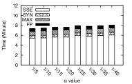
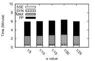
(a) Synthetic dataset (53MB)	(b) Orders dataset (0.325GB)

Figure 6: Time performance for various $\alpha$

Second, to analyze the scalability of our approach, we measure the time performance for various data sizes. The results are shown in Figure 7. It is not surprising that the time performance of all the four steps increases with the data size. We also notice that, on both datasets, the time performance of the SSE step is not linear to the data size. This is due to the fact that the time complexity of the SSE step is quadratic to the number of $EC$s. With the increase of the data size, the average number of $EC$s increases linearly on the synthetic dataset and super-linearly on the Orders dataset. Thus we observe the non-linear relationship between time performance of SSE step and data size. On the synthetic dataset, the dominant time factor is always the time of the SSE step. This is because of the large average number of $EC$s (can be as large as 1 million) and the quadratic complexity of the SSE step. In contrast, the average number of $EC$s is at most $11,828$ on the Orders dataset. So even though the synthetic dataset has fewer and smaller $MAS$s than the Orders dataset, the vast difference in the number of $EC$s makes the SSE step takes the majority of the time performance on the synthetic dataset.

To sum up the observations above, our $F^{2}$ approach can be applied on the large datasets with high security guarantee, especially for the datasets that have few number of $EC$s on the $MAS$s. For instance, it takes around 30 minutes for $F^{2}$ to encrypt the Orders dataset of size 1GB with security guarantee of $\alpha=0.2$.

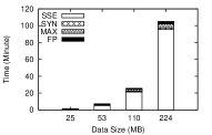
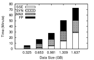
(a) Synthetic dataset ($\alpha$=0.25)	(b) Orders dataset ($\alpha$=0.2)

Figure 7: Time performance for various data sizes

(a) Synthetic dataset ($\alpha$=0.25)	(b) Orders dataset ($\alpha$=0.2)

Figure 8: Time performance Comparison

We also compare the time performance of $F^{2}$ with the two baseline methods. The result is shown in Figure 8. It is not surprising that $F^{2}$ is slower than AES, as it has to handle with the FD-preserving requirement. On the other hand, even though $F^{2}$ has to take additional efforts to be FD-preserving (e.g., finding $MASs$, splitting and scaling, etc.), its time performance is much better than Paillier. This shows the efficiency of our probabilistic encryption scheme. It is worth noting that on the Orders dataset, Paillier takes 1247.27 minutes for the data of size 0.325GB, and cannot finish within one day when the data size reaches 0.653GB. Thus we only show the time performance of Paillier for the data size that is below 0.653GB.

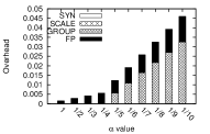
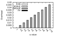
(a) Various $\alpha$ values	(b) Various $\alpha$ values
(Customer 73MB)	(Orders 0.325GB)
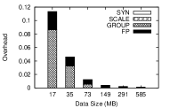
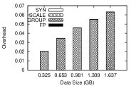
(c) Various data size	(d) Various data size
(Customer $\alpha=0.2$)	(Orders $\alpha$=0.2)

Figure 9: Amounts of Artificial Records Added by $F^{2}$

5.3 Amounts of Artificial Records

In this section, we measure the amounts of the artificial records added by $F^{2}$ on both the Orders and Customer datasets. We measure the amounts of the artificial records added by Step 2.1 grouping (GROUP), Step 2.2 splitting-and-scaling encryption (SCALE), Step 3 conflict resolution (SYN), and Step 4 eliminating false positive FDs (FP) individually. For each step, we measure the data size before and after the step, let them be $s$ and $s^{\prime}$, and calculate the space overhead $r=\frac{s^{\prime}-s}{s}$.

On the Customer dataset, we measure the overhead under various $\alpha$ values in Figure 9 (a). We observe that the GROUP and FP steps introduce most of the overhead. The overhead increases when $\alpha$ decreases, since smaller $\alpha$ value requires larger $ECGs$, and thus more collision-free equivalence classes. But in general, the overhead is very small, always within in 5%. This is because the domain size of the attributes in $MAS$s of the Customer dataset is large. For instance, both the C_Last and C_Balance attribute have more than 4,000 unique values across 120,000 records. Under such setting, different $MASs$ are unlikely collide with each other. As a consequence, the number of artificial records added by the GROUP step is very small. When $\alpha<0.2$, the GROUP step does not even introduce any overhead. The overhead brought by the FP step increases with the decrease of $\alpha$ value. This is because for each maximum false positive FD, $F^{2}$ inserts $2k$ artificial records, where $k=\lceil\frac{1}{\alpha}\rceil$. As $k$ increases, the number of inserted records decreases. But even for small $\alpha$ value such as $\frac{1}{10}$, the overhead brought by the FP step is still very small (around 1.5%). In any case, the space overhead of $F^{2}$ on the Customers dataset never exceeds 5%. We also measure the space overhead with various $\alpha$ values on the Orders dataset. The result is shown in Figure 9 (b). First, the GROUP step adds dominant amounts of new records. The reason is that the domain size of attributes in $MAS$s on the Orders dataset is very small. For example, among the 1.5 million records, the OrderStatus and OrderPriority attributes only have 3 and 5 unique values respectively. Therefore the $ECs$ of these attributes have significant amounts of collision. This requires $F^{2}$ to insert quite a few artificial records to construct the $ECGs$ in which $ECs$ are collision-free. Nevertheless, the amounts of artificial records is negligible compared with the number of original records. The space overhead is 4.5% at most.

In Figure 9 (c) and (d), we show the space overhead of both datasets of various sizes. On the Customer dataset, the overhead reduces with the increase of data size. Such overhead decreases for both GROUP and FP steps. Next we give the reasons. Regarding the GROUP step, this is because in the Customer dataset, the collision between $ECs$ is small. It is more likely that the GROUP step can find collision-free $ECs$ to form the $ECG$s, and thus smaller number of the injected artificial records. Regarding the FP step, its space overhead decreases when the data size grows is due to the fact that the number of artificial records inserted by the FP step is independent of the data size. This makes the number of artificial records constant when the data size grows. Therefore, the overhead ratio decreases for larger datasets. On the Orders dataset, again, the GROUP step contributes most of the injected artificial records. However, contrary to the Orders dataset, the overhead increases with the data size. This is because the $ECs$ of Orders have significant amounts of collision. Thus, the number of $ECs$ increases quadratically with the dataset size. Therefore, the space overhead of the GROUP step increases for larger datasets.

Combining the observations above, our $F^{2}$ method introduces insignificant amounts of artificial records. For instance, the amounts of artificial records takes at most 6% for the Orders dataset, and 12% for the Customer dataset.

5.4 Outsourcing VS. Local Computations

First, we compare the data owner’s performance of finding $FDs$ locally and encryption for outsourcing. We implemented the TANE algorithm [16] and applied it on our datasets. First, we compare the time performance of finding $FDs$ locally (i.e. applying TANE on the original dataset $D$) and outsourcing preparation (i.e., encrypting $D$ by $F^{2}$). It turns out that finding $FDs$ locally is significantly slower than applying $F^{2}$ on the synthetic dataset. For example, TANE takes 1,736 seconds on the synthetic dataset whose size is 25MB to discover FDs, while $F^{2}$ only takes 2 seconds.

(a) Customer dataset (73MB)	(b) Orders dataset (0.325GB)

Figure 10: Dependency Discovery Time Overhead

Second, we compare the performance of discovering $FD$s from the original and encrypted data, for both Customer and Orders datasets. We define the dependency discovery time overhead $o=\frac{T^{\prime}-T}{T}$, where $T$ and $T^{\prime}$ are the time of discovering $FDs$ from $D$ and $\hat{D}$ respectively. The result is shown in Figure 10. For both datasets, the time overhead is small. It is at most 0.4 for the Customers dataset and 0.35 for the Orders dataset. Furthermore, the discovery time overhead increases with the decrease of $\alpha$ value. This is because with smaller $\alpha$, the GROUP and FP steps insert more artificial records to form $ECG$s for higher security guarantee. Consequently the FD discovery time increases. This is the price to pay for higher security guarantee.

6 Related Work

Data security is taken as a primary challenge introduced by the database-as-a-service ($DaS$) paradigm. To protect the sensitive data from the $DaS$ service provider, the client may transform her data so that the server cannot read the actual content of the data outsourced to it. A straightforward solution to data transformation is to encrypt the data while keeping the decryption key at the client side. Hacigumus et al. [14] is one of the pioneering work that explores the data encryption for the $DaS$ paradigm. They propose an infrastructure to guarantee the security of stored data. Different granularity of data to be encrypted, such as row level, field level and page level, is compared. Chen et al. [13] develop a framework for query execution over encrypted data in the $DaS$ paradigm. In this framework, the domain of values of each attribute is partitioned into some bucket. The bucket ID which refers to the partition to which the plain value belongs serves as an index of ciphertext values. Both encryption methods are vulnerable against the frequency analysis attack as they only consider one-to-one substitution encryption scheme. Curino et al. [7] propose a $DaS$ system that provides security protection. Many cryptographic techniques like randomized encryption, order-preserving encryption and homomorphic encryption are applied to provide adjustable security. CryptDB [25] supports processing queries on encrypted data. It employs multiple encryption functions and encrypts each data item under various sequences of encryption functions in an onion approach. Alternatively, Cipherbase [1] exploits the trusted hardware (secure co-processors) to process queries on encrypted data. These cryptographic techniques are not FD-preserving.

Data encryption for outsourcing also arises the challenge of how to perform computations over the encrypted data. A number of privacy-preserving cryptographic protocols are developed for specific applications. For example, searchable encryption [29, 5] allows to conduct keyword searches on the encrypted data, without revealing any additional information. However, searchable encryption does not preserve FDs. Homomorphic encryption [28] enables the service provider to perform meaningful computations on the data, even though it is encrypted. It provides general privacy protection in theory, but it is not yet efficient enough for practice [22].

Integrity constraints such as FDs are widely used for data cleaning. There have been very few efforts on finding data integrity constraints and cleaning of inconsistent data in private settings. Talukder et al. [30] consider a scenario where one party owns the private data quality rules (e.g., $FDs)$ and the other party owns the private data. These two parties wish to cooperate by checking the quality of the data in one party’s database with the rules discovered in the other party’s database. They require that both the data and the quality rules need to remain private. They propose a cryptographic approach for FD-based inconsistency detection in private databases without the use of a third party. The quadratic algorithms in the protocol may incur high cost on large datasets [30]. Barone et al. [2] design a privacy-preserving data quality assessment that embeds data and domain look-up table values with Borugain Embedding. The protocol requires a third party to verify the (encrypted) data against the (encrypted) look-up table values for data inconsistency detection. Both work assume that the data quality rules such as $FDs$ are pre-defined. None of these work can be directly applied to our setting due to different problem definition and possibly high computational cost.

Efficient discovery of FDs in relations is a well-known challenge in database research. Several approaches (e.g., TANE [16], FD_MINE [31], and FUN [23]) have been proposed. [24] classifies and compares seven FD discovery algorithms in the literature. [19] presents an excellent survey of FD discovery algorithms.

7 Conclusion and Discussion

In this paper, we presented $F^{2}$ algorithm that is FD-preserving and frequency-hiding. It can provide provable security guarantee against the frequency analysis attack, even under the Kerckhoffs’s principle. Our experiment results demonstrate the efficiency of our approach.

We acknowledge that $F^{2}$ does not support efficient data updates, since it has to apply splitting and scaling (Step 2.2) from scratch if there is any data update. For the future work, we will consider how to address this important issue. Another interesting direction is to extend to malicious attackers that may not follow the outsourcing protocol and thus cheats on the data dependency discovery results. The problem of verifying whether the returned FDs are correct is challenging, given the fact that the data owner is not aware of any $FD$ in the original dataset.

8 Acknowledgement

This material is based upon work supported by the National Science Foundation under Grant SaTC-1350324 and SaTC-1464800. Any opinions, findings, and conclusions or recommendations expressed in this material are those of the author(s) and do not necessarily reflect the views of the National Science Foundation.

References

- [1] A. Arasu, S. Blanas, K. Eguro, R. Kaushik, D. Kossmann, R. Ramamurthy, and R. Venkatesan. Orthogonal security with cipherbase. In CIDR, 2013.
- [2] D. Barone, A. Maurino, F. Stella, and C. Batini. A privacy-preserving framework for accuracy and completeness quality assessment. Emerging Paradigms in Informatics, Systems and Communication, 2009.
- [3] C. Batini, M. Lenzerini, and S. B. Navathe. A comparative analysis of methodologies for database schema integration. ACM computing surveys (CSUR), 18(4):323–364, 1986.
- [4] P. Bohannon, W. Fan, F. Geerts, X. Jia, and A. Kementsietsidis. Conditional functional dependencies for data cleaning. In International Conference on Data Engineering, 2007.
- [5] D. Boneh, G. Di Crescenzo, R. Ostrovsky, and G. Persiano. Public key encryption with keyword search. In Advances in Cryptology, 2004.
- [6] L. Chiticariu, M. A. Hernández, P. G. Kolaitis, and L. Popa. Semi-automatic schema integration in clio. In Proceedings of the VLDB Endowment, pages 1326–1329, 2007.
- [7] C. Curino, E. Jones, R. A. Popa, N. Malviya, E. Wu, S. Madden, H. Balakrishnan, and N. Zeldovich. Relational cloud: A database service for the cloud. In 5th Biennial Conference on Innovative Data Systems Research, 2011.
- [8] G. I. Davida, D. L. Wells, and J. B. Kam. A database encryption system with subkeys. ACM Transactions on Database Systems (TODS), 6(2):312–328, 1981.
- [9] B. Dong, R. Liu, and W. H. Wang. Prada: Privacy-preserving data-deduplication-as-a-service. In Proceedings of the International Conference on Information and Knowledge Management, pages 1559–1568, 2014.
- [10] W. Fan, F. Geerts, J. Li, and M. Xiong. Discovering conditional functional dependencies. IEEE Transaction of Knowledge and Data Engineering, 23(5):683–698, 2011.
- [11] S. Goldwasser and S. Micali. Probabilistic encryption. Journal of Computer and System Sciences, 1984.
- [12] D. Gunopulos, R. Khardon, H. Mannila, S. Saluja, H. Toivonen, and R. S. Sharma. Discovering all most specific sentences. ACM Transactions on Database Systems (TODS), 28(2):140–174, 2003.
- [13] H. Hacigumus, B. Iyer, C. Li, and S. Mehrotra. Executing sql over encrypted data in the database-service-provider model. In Proceedings of the International Conference on Management of Data, pages 216–227, 2002.
- [14] H. Hacigumus, B. Iyer, and S. Mehrotra. Providing database as a service. In Proceedings of International Conference on Data Engineering. IEEE, 2002.
- [15] A. Heise, J.-A. Quiané-Ruiz, Z. Abedjan, A. Jentzsch, and F. Naumann. Scalable discovery of unique column combinations. Proceedings of the VLDB Endowment, 7(4):301–312, 2013.
- [16] Y. Huhtala, J. Kärkkäinen, P. Porkka, and H. Toivonen. Tane: An efficient algorithm for discovering functional and approximate dependencies. The computer journal, 42(2):100–111, 1999.
- [17] J. Katz and Y. Lindell. Introduction to modern cryptography: principles and protocols. CRC press, 2007.
- [18] F. Kerschbaum. Frequency-hiding order-preserving encryption. In Proceedings of the Conference on Computer and Communications Security, 2015.
- [19] J. Liu, J. Li, C. Liu, and Y. Chen. Discover dependencies from data a review. IEEE Transactions on Knowledge & Data Engineering, (2):251–264, 2010.
- [20] B. Marnette, G. Mecca, and P. Papotti. Scalable data exchange with functional dependencies. Proceedings of the VLDB Endowment, 3(1-2):105–116, 2010.
- [21] R. J. Miller, Y. E. Ioannidis, and R. Ramakrishnan. The use of information capacity in schema integration and translation. In VLDB, 1993.
- [22] M. Naehrig, K. Lauter, and V. Vaikuntanathan. Can homomorphic encryption be practical? In Proceedings of the 3rd ACM Cloud Computing Security Workshop, pages 113–124, 2011.
- [23] N. Novelli and R. Cicchetti. Fun: An efficient algorithm for mining functional and embedded dependencies. In Database Theory (ICDT). 2001.
- [24] T. Papenbrock, J. Ehrlich, J. Marten, T. Neubert, J.-P. Rudolph, M. Schönberg, J. Zwiener, and F. Naumann. Functional dependency discovery: An experimental evaluation of seven algorithms. Proceedings of the VLDB Endowment, 8(10), 2015.
- [25] R. A. Popa, C. Redfield, N. Zeldovich, and H. Balakrishnan. Cryptdb: Processing queries on an encrypted database. Communications of the ACM, 55(9):103–111, 2012.
- [26] T. Sanamrad, L. Braun, D. Kossmann, and R. Venkatesan. Randomly partitioned encryption for cloud databases. In Data and Applications Security and Privacy XXVIII, pages 307–323. 2014.
- [27] C. E. Shannon. Communication theory of secrecy systems*. Bell System Technical Journal, 1949.
- [28] N. P. Smart and F. Vercauteren. Fully homomorphic encryption with relatively small key and ciphertext sizes. In Public Key Cryptography (PKC). 2010.
- [29] D. X. Song, D. Wagner, and A. Perrig. Practical techniques for searches on encrypted data. In Proceedings of IEEE Symposium on Security and Privacy, pages 44–55, 2000.
- [30] N. Talukder, M. Ouzzani, A. K. Elmagarmid, and M. Yakout. Detecting inconsistencies in private data with secure function evaluation. Technical report, Purdue University, 2011.
- [31] H. Yao, H. J. Hamilton, and C. J. Butz. Fd_mine: discovering functional dependencies in a database using equivalences. In IEEE International Conference on Data Mining, pages 729–732, 2002.