Shaping the GeV-spectra of bright blazars

Abstract

Aims. The non-thermal spectra of jetted active galactic nuclei (AGN) show a variety of shapes and degree of curvature in their low- and high energy components. From some of the brightest Fermi-LAT blazars, prominent spectral breaks at a few GeV have been regularly detected, which is inconsistent with conventional cooling effects. We study the effects of continuous time-dependent injection of electrons into the jet with differing rates, durations, locations, and power-law spectral indices, and evaluate its impact on the ambient emitting particle spectrum that is observed at a given snapshot time in the framework of a leptonic blazar emission model. With this study, we provide a basis for analyzing ambient electron spectra in terms of injection requirements, with implications for particle acceleration modes.

Methods. The emitting electron spectrum is calculated by Compton cooling the continuously injected electrons, where target photons are assumed to be provided by the accretion disk and broad line region (BLR). From this setup, we calculate the non-thermal photon spectra produced by inverse Compton scattering of these external target radiation fields using the full Compton cross-section in the head-on approximation.

Results. By means of a comprehensive parameter study we present the resulting ambient electron and photon spectra, and discuss the influence of each injection parameter individually. We found that varying the injection parameters has a notable influence on the spectral shapes, which in turn can be used to set interesting constraints on the particle injection scenarios. By applying our model to the flare state spectral energy distribution (SED) of 3C 454.3, we confirm a previous suggestion that explained the observed spectral changes at a few GeV by a combination of the Compton-scattered disk and BLR radiation. We determine the required injection parameters for this scenario. We also show that this spectral turn-over can also be understood as Compton-scattered BLR radiation only, and provide the corresponding injection parameters. Here the spectral turn-over is explained by a corresponding break in the ambient electron spectrum. In a similar way, we also applied our model to the FSRQ PKS 1510-089, and present two possible model fits. Here, the GeV-spectrum is either dominated by Compton-scattered accretion disk radiation or is a combination of Compton-scattered disk and BLR radiation. We provide the required injection parameters for these fits. In all four scenarios, we found that impulsive particle injection is disfavored.

Conclusions. The presented injection model that is embedded in a leptonic blazar emission model for external Compton-loss dominated jets of AGN aims towards bridging jet emission with acceleration models using a phenomenological approach. Blazar spectral data can be analyzed with this model to constrain injection parameters, in addition to the conventional parameter values of steady-state emission models, if sufficient broad multifrequency coverage is provided.

1 Introduction

Jetted active Galactic Nuclei (AGN) comprise the most numerous variable source population in the $\gamma$-ray sky (e.g., 2013ApJ...771...57A). Their jets are considered as the site of intense broadband emission, with apparently random flaring events, shich cover the electromagnetic band from the radio up to GeV, or TeV energies. Variability timescales for this continuum emission range from months (radio) down to few minutes (TeV). Their broadband spectral energy distribution (SED) can be described as having two broad components, with the lower energy component usually attributed to synchrotron radiation from a population of relativistic electrons in the magnetized emission region. The origin of the photons of the higher energy component is still under debate, and strongly depends on the relativistic particle content of the jet (e.g., 2013APh....43..103R). In many cases, it is only by considering leptonic processes together with external target photon fields that can lead to snapshot or time-averaged SEDs that are in agreement with the corresponding multifrequency observations (e.g., 2013ApJ...768...54B). An often used approach for calculating these SEDs is based on an ad hoc assumption of the emitting electron spectrum as having log-parabolic shapes, (broken) power laws with possible exponential cutoffs, and with the minimum and maximum electron energies, energy of possible breaks and power law indices or curvature of this spectrum as free parameters (e.g., 2009ApJ...692...32D, 2010ApJ...714L.303F, 2014ApJ...782...82D).

The observation of spectral breaks in the high energy photon spectra of bright flat spectrum radio quasars (FSRQ) was among the first findings of the Fermi-LAT in the extragalactic $\gamma$-ray sky (2009ApJ...699..817A; 2010ApJ...710.1271A, and confirmed subsequently in 2011ApJ...743..171A). Typically, bright FSRQs (and also some low frequency peaked-BL Lacs (LBLs) and intermediate frequency peaked-BL Lacs (IBLs)) show $\gamma$-ray spectra that can be described phenomenologically either by broken power laws or log-parabolas with strong concave curvature (2014MNRAS.441.3591H) between 1 and 10 GeV, which is too low to be caused by absorption in the extragalactic background light (e.g., 2010ApJ...723.1082A), and with a power-law index change much larger than expected from cooling ($\Delta\Gamma=0.5$). For example, the turn-over in the GeV spectra of FSRQ 3C 454.3 is located at $\sim 2.5$ GeV with a power law index change of about $\Delta\Gamma=1.1\pm 0.1$. The break energy does not seem to be correlated with the $\gamma$-ray luminosity. Several scenarios have been proposed to explain these breaks. These range from photon pair production in the broad-line region of the source (BLR; 2010ApJ...717L.118), to a two-component $\gamma$-ray spectrum (2010ApJ...714L.303F), or GeV breaks in the photon spectra owing to corresponding breaks in the electron spectra (2010ApJ...710.1271A).

Some recent studies, however, have cast doubt on the internal absorption scenario, which would predict well-defined break energies in the AGN’s source frame. 2012ApJ...761....2H did not find such universal values of the break energies. 2015MNRAS.449.2901K described the occurence of spectral breaks, which were investigated from a set of 40 bright LAT-blazars as “random”. In fact they report a tendency for short duration flares to possess stronger curvature than those hat are integrated over a longer timescale. The other two non-absorption scenarios mentioned above invoke ad hoc broken power-law particle spectra. 2009MNRAS.397..985G show that Klein-Nishina or simple cooling effects cannot explain the strength and shape of the observed peaks (see however, 2013ApJ...771L...4C who propose a high-energy cutoff at GeV energies from Klein-Nishina effects in scattering Ly_α photons).

Using the ambient particle spectrum as an input parameter, however, broadly ignores the build-up of this emitting particle spectrum that is impacted by the various particle energy losses, and gains through particle energization mechanisms which, in general, requires a time-dependent treatment of the problem. As a consequence one can not gain much information on the particle acceleration mechanisms at work in these environments from modeling broadband SEDs this way.

In the present work we attempt to improve on this situation by studying the impact of various injection scenarios of relativistic particles on the resulting emitting particle and photon spectrum. Specifically, we calculate the ambient particle spectrum that results from injection during a finite time range in the past, and viewed at a given (snapshot) time. Comparing to the broken power-law, emitting-particle spectra, which are required in broadband modeling of blazar snapshot SEDs, will then help us draw inferences on the required particle acceleration mechanisms.

In this sense, our approach differs from works which directly implement a specific acceleration mechanism into an emission code (e.g., 2014JHEAp...1...63D).

We restrict ourselves to leptonic emission processes in blazar jets here where external photon fields, such as accretion disk radiation and radiation partly re-scattered at the BLR, present the dominant target for particle-photon interactions. This setup is expected to be suitable for application to those radio-loud jetted AGN, which show a strong accretion disk radiation field, such as FSRQs and LBLs. The analog procedure, including hadronic interactions as well, is more complex and will be postponed to a subsequent paper.

We aim to explain the observed breaking spectra at GeV-energies, and hence focus here on steep spectrum LAT-AGN. This is unlike 2014ApJ...790...45P, whose study on spectral shapes is based on a data set in which those periods are exclusively considered where the sources emitted significant $>10$ GeV photons and are therefore associated with hard $\gamma$-ray spectrum-flaring events. 2014JHEAp...1...63D complemented their time-dependent leptonic blazar emission code with an implementation of a Fermi-II acceleration scenario, in addition to time-dependent particle “pick-up”, with the goal of identifying observational signatures for the origin of flares. Hence they studied the effect of a perturbation of various input parameters that could potentially be associated with causing outbursts on top of a steady-state situation. They explored observational signatures such as correlations between lightcurves at different frequencies, possible time lags, etc. Our present work attempts to explore the impact of a specific injection history on the resulting high-energy spectrum thereby offering an alternative explanation for the often observed strong breaks in bright FSRQ spectra at GeV-energies.

Section 2 of this paper describes the emission model used here (an external inverse Compton emission model that broadly follows 1993ApJ...416..458D, 2009ApJ...692...32D), and the calculation of the emitting electron spectrum, which is the result of radiative losses that impact upon an electron population that has been continuously injected while propagating along the jet. Such continuously injected electron spectra, like the one we use in this work, were first proposed by 2000MNRAS.312..177M. We present a detailed parameter study in Sect. 3, and summarize and discuss the results of our work in Sect. 4.

2 Model

2.1 Basic model

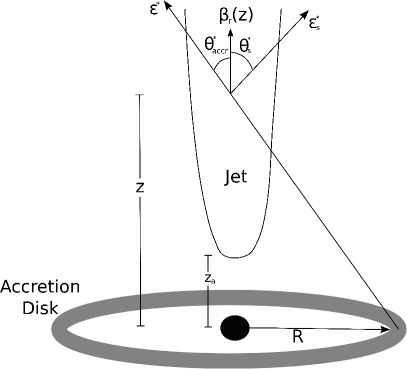
Figure 1: Geometry of the blazar jet model considered in this work (Figure adapted from 1993ApJ...416..458D).

We consider the AGN to be powered by accretion onto a supermassive Schwarzschild black hole of mass $M_{\rm BH}$. The central black hole is surrounded by a Shakura-Sunyaev accretion disk (1973A&A....24..337S). Accretion disk photons, with energy $\varepsilon^{*}$, enter the jet under the angle $\theta^{*}_{accr}$. These photons are scattered into the angle $\theta_{s}^{*}$ with scattered photon energy $\varepsilon_{s}^{*}$, by the jet electrons. The plasma outflow of the jet starts at a distance $z_{0}$ from the central black hole and flows along the symmetry axis of the system with bulk Lorentz factor $\Gamma$ and the velocity $\beta_{\Gamma}c$, where $\beta_{\Gamma}=\sqrt{1-1/\Gamma^{2}}$. Figure 1 illustrates the basic model used in this work. Other than in the model of 1993ApJ...416..458D, electrons are injected continuously along the jet axis between heights $z_{a}$ and $z_{b}$ with a time-dependent injection rate $\propto z(t)^{-\alpha}$, with $\alpha$ being a free parameter. We consider cooling of the the injected electrons as being dominantly the result of inverse Compton losses on external target radiation fields. Two target photon fields are considered here: the aforementioned accretion disk radiation, which generally enters the jet under small angles $\theta^{*}_{accr}$, and the accretion disk radiation that has been backscattered by the BLR. Most of this backscattered radiation enters the jet under angles $\theta^{*}>90^{\circ}$, which leads to a different scattering behavior. Because the two target photon fields have different angular distributions in the jet frame, the inverse Compton scattered photon distributions that are produced by each of the target photon fields shows correspondingly different spectral shapes. The BLR model used here largely follows 2009ApJ...692...32D and is described in Sect. 2.2.1.

In the following, quantities with asterisks are in the rest frame of the accretion disk. All energies are in units of the electron rest mass $m_{e}c^{2}$.

2.2 Compton cooling rates

We consider Compton cooling of electrons in the comoving frame of the jet. This radiative cooling rate is dependent on the differential Compton photon production rate,

rCl ˙n(ε_s,Ω_s,z) & = c∫^∞_0 dε∮dΩ∫^∞_1 dγ∮dΩ_e (1-β⋅cos(ψ))
⋅n_ph(ε,Ω,z) ⋅n_e(γ,Ω_e) dσCdεsdΩs,

which is dependent on

• $n_{\rm{ph}}(\varepsilon,\Omega,z)$, the photon density of the target photon field at solid angle ($\Omega$), energy ($\varepsilon$) and position ($z$) along the jet axis,

• $n_{e}(\gamma,\Omega_{e})$, the electron density at electron Lorentz factor $\gamma$ and the solid angle ($\Omega_{e}$),

• the differential Compton scattering cross section $\frac{d\sigma_{C}}{d\varepsilon_{s}d\Omega_{s}}$.

Here, $\cos(\psi)=\mu\mu_{e}+\sqrt{(1-\mu^{2})}\sqrt{1-\mu_{e}^{2}}\cos(\phi-\phi_{e})$ describes the three-dimensional collision angle.

We assume that the electron density is isotropic in the comoving frame of the jet, $n_{e}(\gamma,\Omega_{e})=\frac{n_{e}(\gamma)}{4\pi}$. To calculate the energy loss rate, we set $n_{e}(\gamma)=\delta(\gamma-\bar{\gamma})$, where $\delta()$ denotes the Delta distribution. By only considering relativistic electrons, the assumption $\gamma\gg 1$ is justified. Furthermore, we use the Thomson approximation for the differential cross-section with the $\delta$-approximation in the head-on case:

$$\frac{d\sigma}{d\varepsilon_{s}d\Omega_{s}}=\sigma_{T}\delta[\varepsilon_{s}-\gamma^{2}\varepsilon(1-\beta\cos(\psi))]\delta(\Omega_{s}-\Omega_{e})$$ (1)

where $\sigma_{T}$ denotes the Thomson cross-section. This is valid as long as $\varepsilon^{\prime}\equiv\gamma\varepsilon(1-\cos(\psi))\leq 1$. For $\varepsilon^{\prime}>1$ (Klein-Nishina regime) we assume that the cross-section is zero when calculating the cooling rates, since the Klein-Nishina cross-section declines rapidly at high energies.

With these approximations, the integrations over $\Omega_{e}$ and $\varepsilon$ are trivial. To achieve further simplification, we average the azimuthally symmetric problem over $\phi$ implying $\langle\cos(\psi)\rangle=\mu\mu_{s}$ .

The integrations then lead to

$$\dot{n}(\varepsilon_{s},\mu_{s},z)=\frac{c\sigma_{T}}{4\pi}\int^{1}_{-1}d\mu\,\gamma^{-2}\cdot n_{\rm{ph}}\left(\frac{\varepsilon_{s}}{\gamma^{2}(1-\beta\cos(\psi))},\mu,z\right).$$ (2)

To make progress in calculating the scattered differential photon production rate the two differential target photon densities $n_{\rm{ph}}$ (in the comoving frame) are required. Their calculations are shown in the following two sections.

2.2.1 BLR target photon density

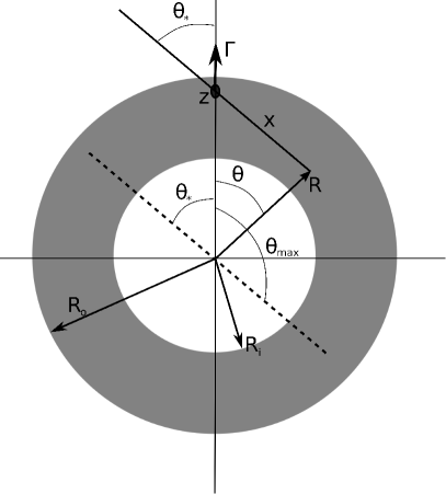
Figure 2: Our BLR model consists of a spherically symmetric shell of gas between $R_{i}$ and $R_{o}$ and a density gradient $\zeta$ with $n_{e}(R)\propto R^{\zeta}$ (Figure adapted from 2009ApJ...692...32D).

.

Figure 2 sketches the BLR model used here, mainly following 2009ApJ...692...32D, where the BLR target photon field is the result of reprocessing the accretion disk radiation and with any direct BLR line emissivity being neglected. For the purpose of calculating the target photon field re-scattered at the BLR (BLR target photon field), we consider the central source as an isotropically emitting point source.

An anisotropic central source would slightly increase the energy density caused by the BLR in the jet-frame with distance from the illuminating disk (1996MNRAS.280...67G).

The central source radiation is isotropically Thomson-scattered by material of the BLR, back to a distance $z$ (above the black hole) on the jet axis. We consider a spherically symmetric shell of thin gas for the scattering BLR material with a density gradient inside this shell (see Fig. 2). Taking into account a clumpy BLR, instead, would require the introduction of further free parameters (cloud radius distribution) while the expected impact on the distribution of the reprocessed radiation likely stays small for not too large cloud sizes: one would expect additional inhomogenities to some extent on top of an R-dependence from the BLR density gradient.

The calculations here are all carried out in the rest frame of the BLR.

The Thomson-scattered photon density is obtained by

$$n^{\rm{BLR}}_{\rm{ph}}(\varepsilon_{*};z)=\int dV\frac{\dot{n}(\varepsilon_{*};\@vec{R})}{4\pi x^{2}c}.$$ (3)

Here $x^{2}=R^{2}+z^{2}-2zR\cos(\theta)$, and $\dot{n}(\varepsilon_{*};\@vec{R})$, the differential BLR-scattered photon density rate, is given by

$$\dot{n}(\varepsilon_{*};\@vec{R})=\frac{\dot{N}_{\rm{ph}}(\varepsilon_{*})\sigma_{T}n_{e}^{BLR}(R)}{4\pi R^{2}},$$ (4)

where

• $\dot{N}_{\rm{ph}}(\varepsilon_{*})$ is the central source photon production rate,

• $\sigma_{T}n_{e}^{BLR}(R)$ gives the fraction of the incoming flux that is scattered,

• $\frac{1}{4\pi R^{2}}$ is the geometric dilution from an isotropic source.

With spherical coordinates and Eq.(4), Eq.(3) we find:

$$n^{\rm{BLR}}_{\rm{ph}}(\varepsilon_{*};z)=\frac{\sigma_{T}\dot{N}_{\rm{ph}}(\varepsilon_{*})}{8\pi c}\int_{-1}^{1}d\mu\int_{0}^{\infty}dR\frac{n_{e}(R)}{x^{2}}.$$ (5)

Since inverse Compton scattering is angle dependent, we need the angle-dependent target photon spectrum. With $\delta(\mu_{*}-\bar{\mu}_{*})$, $\mu_{*}=\cos\ \theta_{*}$ and by changing the variables to $g=R/z$ we get

rCl n^BLR_ph(ε_*;z) & = σT˙Nph(ε*)8πc z
⋅∫_-μ^*^1 dμ∫_0^∞ dg ne(gz) δ[μ*-¯μ*(μ,g)]g2+1-2gμ.

We use the law of sines $R^{2}(1-\mu^{2})=x^{2}(1-\mu_{*}^{2})$ to calculate the angle $\mu_{*}$ under which the scattered photons reach the point $z$:

$${\bar{\mu}}_{*}(\mu,g)=\frac{\pm(1-g\mu)}{\sqrt{(1+g^{2}-2g\mu)}}.$$ (6)

$\bar{\mu}_{*}(\mu,g)$ defines a line. If the scattering process takes place on that line, a photon emitted into the angle $\mu$ arrives with angle $\mu_{*}$ at point $z$. Formally, there are two solutions with the positive one being the physically relevant one for the already $\phi$-integrated quantity ${\bar{\mu}}_{*}(\mu,g)$.

Carrying out the integration we find:

$$n^{\rm{BLR}}_{\rm{ph}}(\varepsilon_{*},\mu_{*};z)=\frac{\sigma_{T}\dot{N}_{\rm{ph}}(\varepsilon_{*})}{8\pi c}\frac{\Pi(\mu_{*},z)}{z},$$ (7)

where

$$\Pi(\mu_{*},z)\equiv\int^{1}_{-\mu_{*}}d\mu\ n_{e}(\bar{g}z)\frac{\sqrt{1+\bar{g}^{2}-2\bar{g}\mu}}{\bar{g}(1-\mu^{2})}$$

and

$$\bar{g}=\bar{g}(\mu,\mu_{*})\equiv\frac{-\mu(1-\mu_{*}^{2})+\mu_{*}\sqrt{(1-\mu^{2})(1-\mu_{*}^{2})}}{\mu_{*}^{2}-\mu^{2}}.$$

Here $\bar{g}$ describes the radius $R$ at which the photons, emitted into the angle $\mu$, have to be scattered to end up in $\mu_{*}$. $n_{e}(\bar{g}z)$ is the electron density at the scattering point. This means $\Pi(\mu_{*},z)$ gives a measure for the total number of photons that end up in the angle element $\mu_{*}$ at point $z$ along the jet axis.

$\Pi$ cannot be solved analytically, but numerically. The results of these calculations, which we find in agreement with 2009ApJ...692...32D, are shown in Fig. 3. The figure shows the angular distribution of the BLR photons for different positions $z$. For $z\geq R_{o}$ there are no incoming photons from the front ($\mu_{*}<0$) since there is no scattering BLR material in front of $z$.

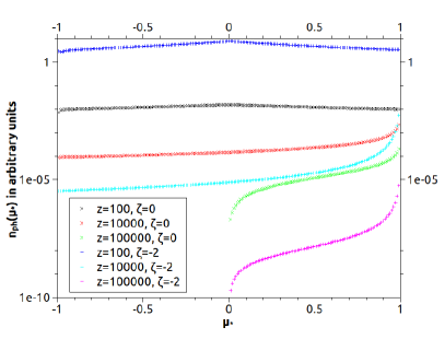
Figure 3: Angle dependence of $n_{\rm{ph}}^{BLR}$ for a BLR extending from $10^{2}$ to $10^{5}$ $R_{g}$ for different values of $z$ (in $R_{g}$) and $\zeta$, in agreement with 2009ApJ...692...32D.

The central source photon-production rate $\dot{N}_{\rm{ph}}(\varepsilon_{*})$ is calculated by assuming that this photon source emits a monochromatic spectrum with luminosity $L_{0}$:

$$\dot{N}_{\rm{ph}}(\varepsilon_{*})=\frac{L_{0}\delta(\varepsilon_{*}-\varepsilon_{0*})}{m_{e}c^{2}\varepsilon_{*}}.$$ (8)

Here $L_{0}=L_{\rm{edd}}l_{\rm{edd}}$, with $L_{\rm{edd}}$ the Eddington luminosity of the black hole. 2008MNRAS.386..945T have shown that the BLR radiation, simulated with the photoionization code CLOUDY, as the target field for inverse Compton scattering can be adequately approximated by a blackbody with a peak at 1.5 times the Ly_α-frequency , when considering the IC spectrum above a few keV. Afterwards, we approximate this blackbody with a monochromatic spectrum.

The resulting BLR target photon density is

$$n^{\rm{BLR}}_{\rm{ph}}(\varepsilon_{*},\mu_{*};z)=\frac{\sigma_{T}L_{\rm{edd}}l_{\rm{edd}}\delta(\varepsilon_{*}-\varepsilon_{0*})}{8\pi m_{e}c^{3}\varepsilon_{*}}\frac{\Pi(\mu_{*},z)}{z}.$$ (9)

To transform this into the comoving frame we use $\varepsilon_{*}=\Gamma\varepsilon(1+\beta_{\Gamma}\mu)$ and $\mu_{*}=\frac{(\mu+\beta_{\Gamma})}{1+\beta_{\Gamma}\mu}$, to get

rCl n^BLR_ph(ε,μ;z) & = σTLeddleddδ(Γ(1+βΓμ)(ε-ε0))8πmec3εΓ(1+βΓμ)
⋅Π((μ+βΓ)1+βΓμ,z)z.

2.2.2 Accretion disk target photon density

To calculate the accretion disk photon density in the comoving jet-frame, we follow the procedure outlined in 1993ApJ...416..458D. The accretion disk target photon density at the point $z$ is given by

$$n^{\rm{SSD}}_{\rm{ph}}(\varepsilon_{*},\mu_{*},R;z)=\frac{\dot{N}_{\rm{ph}}(\varepsilon_{*},R)}{4\pi x^{2}c}\frac{\delta(\mu_{*}-\bar{\mu}_{*,accr})}{2\pi},$$ (10)

with

$$\dot{N}_{\rm{ph}}(\varepsilon_{*},R)=\frac{2\pi RF(\varepsilon_{*},R)}{\varepsilon_{*}}$$ (11)

and the surface energy flux for a Shakura-Sunyaev disk is

$$F(R)=\frac{3GM\dot{M}}{8\pi m_{e}c^{2}R^{3}}I(R).$$ (12)

Here $I(R)=1-\sqrt{R_{i}/R}$, $\dot{M}$ is the mass accretion rate and $R_{i}=6R_{g}$ for a Schwarzschild black hole with $R_{g}=GM/c^{2}$ the gravitational radius. In gravitational units, $\tilde{R}=R/R_{g}$, Eq. (12) becomes

$$F(\tilde{R})=\frac{\Phi_{F}}{\tilde{R}^{3}}I(\tilde{R}),$$ (13)

with $\Phi_{F}=8.43\cdot 10^{24}\Psi\mathrm{cm}^{-2}\mathrm{s}^{-1}$ and $\Psi=l_{\rm{edd}}/\epsilon_{f}M_{8}$ where $M_{8}$ is the black hole mass in $10^{8}$ solar masses .

We use a monochromatic approximation for the blackbody radiation that is emitted locally at a specific radius $\tilde{R}$ of the accretion disk. The mean photon energy emitted at a radius $\tilde{R}$ is then given by

$$\bar{\varepsilon}^{*}=2.69\cdot 10^{-4}\tilde{R}^{-3/4}\Psi^{1/4}I(\tilde{R})^{1/4}.$$ (14)

By combining Eq. (11),  (13) and,  (14) we get

$$\dot{N}_{\rm{ph}}(\varepsilon^{*},\tilde{R})=\frac{2\pi R_{g}^{2}\Phi_{F}I(\tilde{R})}{\bar{\varepsilon}^{*}\tilde{R}^{2}}\delta(\varepsilon^{*}-\bar{\varepsilon}^{*}).$$ (15)

After substituting $\dot{N}_{\rm{ph}}$ in Eq.(10) with Eq.(15) and transforming the result into the comoving frame we find

rCl n^SSD_ph(ε,μ,~R;z) & = Rg2ΦFI(~R)4πx2c ~R2¯ε* δ(Γ(1+β_Γμ)(ε-¯ε))
⋅δ(μ-¯μ*,accr-βΓ1-βΓ¯μ*,accr).

2.3 Energy loss and equation of motion

2.3.1 Energy loss in the BLR radiation field

With the differential target photon density, we now calculate the scattered photon density. We use Eq.(3) together with Eq. (2) to calculate $\dot{n}^{\rm{BLR}}(\varepsilon_{s},\mu_{s},z)$. By integrating over all scattering angles $\mathbf{\mu_{s}}$, and all scattering energies $\varepsilon_{s}$, we get the energy-loss rate of a single electron of given $\gamma$:

$$-\dot{\gamma}(\gamma,z)=\int^{1}_{-1}d\mu_{s}\int^{\infty}_{0}d\varepsilon_{s}\;\varepsilon_{s}\cdot\dot{n}^{\rm{BLR}}(\varepsilon_{s},\mu_{s},z).$$ (16)

After integrating over $\varepsilon_{s}$ we get:

rCl -˙γ(γ,z) &= σT2Leddledd⋅γ216 π⋅mec2Γ2 ∫^1_-1 dμ_s ∫^1_-1 dμ  (1-μμs)2(1+βΓμ)2
⋅Π(μ+βΓ1+βΓμ,z)z.

Because the electron energy loss rate depends on $(1-\mu\mu_{s})^{2}/(1+\beta_{\rm{\Gamma}}\mu)^{2}$ photons with incident angles $\mu<0$ contribute more strongly to the electron energy loss rate than photons with incident angles $\mu>0$. The small number of reprocessed BLR photons causes the energy loss due to the BLR to be negligible for the cases that we considered here (see Fig.4).

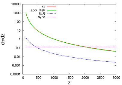
(a) Radiative electron energy loss rates for varying $z$ for electron energy $\gamma=500$ and BLR1 with $\tau_{\rm{BLR}}=0.01$.

(b) Radiative electron energy loss rates for varying $\gamma$ at $z=100$ and BLR1 with $\tau_{\rm{BLR}}=0.01$. BLR shows the BLR energy loss used in our calculations, here we set the energy loss in the Klein-Nishina regime to 0.

Figure 4: Comparison of radiative electron energy-loss rates. Here we choose BLR1 at $z=100$ as an example, while noting that the qualitative picture, with the negligible BLR losses, is the same in all the cases we considered in our study. We compare with synchrotron loss rates for a $B=4.5$G magnetic field.

2.3.2 Energy loss in the accretion disk photon field

The procedure is analogous to the BLR case: We use Eq.(2) to calculate the differential photon production rate for one electron: rCl ˙n^SSD(ε_s,μ_s,R,z) & = σTΦFI(~R)8πx2Rg2~R2¯ε*
⋅δ(Γ(1+β_Γ¯μ)(εsγ2(1-¯μμs)-¯ε)) .

This leads to the energy-loss rate induced by the accretion disk target photons of

rCl -˙γ(γ,z) & = σTΦF8πγ2 ∫_R_i^∞ dR ~R^-2 ~x^2 ∫_0^∞ dε_s  ε_s I(~R)ε*
⋅δ(Γ(1+β_Γ¯μ)(εsγ2(1-¯μμs)-¯ε).

The very good approximation for the solution of Eq. (2.3.2) in the near-field regime ($z<0.1\Gamma^{4}(1+\beta_{\Gamma})^{4}$) is given by 1993ApJ...416..458D, which we use in the following.

2.3.3 Thomson scattering criterion

The energy loss rates are calculated in the Thomson regime, and are therefore only valid for $\varepsilon^{\prime}\equiv\gamma\varepsilon(1-\cos(\psi))\leq 1$ while, in the Klein-Nishina regime, the cross section is set to zero. After transforming the target photon energy $\varepsilon$ into the rest frame of the BLR, we obtain the Thomson limit criterion:

$$\gamma\Gamma\varepsilon_{*}(1-\beta_{\Gamma}\mu_{*})(1-\beta\cos(\psi))<1.$$ (17)

Again, we use the monochromatic approximation for both external target photon fields to confine the range of $\gamma$, where both energy loss rates are in the Thomson regime. Since $1-\beta\cos(\psi)$ can never be larger than 2, the scattering will always be in the Thomson regime if the following relation is fulfilled:

$$2\gamma\Gamma\varepsilon_{*}(1-\beta_{\Gamma}\mu_{*})<1.$$ (18)

The accretion disk photons will mainly enter the jet from behind, i.e. $\mu_{*}\approx 1$. In this case, the Thomson criterion for scattering the accretion disk target photons is:

$$\gamma<\frac{1}{2\Gamma\varepsilon_{*}(1-\beta_{\Gamma})}.$$ (19)

The BLR photons that are most important for the problem will enter the jet from the front, $\mu_{*}\approx-1$. In this case the Thomson criterion changes to:

$$\gamma<\frac{1}{4\Gamma\varepsilon_{*}}.$$ (20)

For larger $\gamma$, the rate of inverse Compton scattering in the BLR reduces to the Klein-Nishina regime, which we neglect in the following. We can neglect the energy loss in the Klein-Nishina regime for the BLR target photons. This neglect is justified since the energy loss owing to the BLR is negligible with respect to the energy loss caused by the accretion disk target photons in the cases that are considered in this work (see Fig.4). In the cases we studied, the accretion disk photons are usually scattered in the Thomson regime.

2.3.4 Omission criterium for synchrotron energy losses

In particular, this work targets accretion radiation-strong blazars such as FSRQs. Here synchrotron energy losses of the charged particles are typically weak when compared to Compton losses (see also Fig.4). In the Thomson limit, synchrotron losses can therefore be neglected when, in the jet-frame, the magnetic field energy density $u^{\prime}_{B}=\frac{B^{2}}{8\pi}$ is much lower than the sum of all target photon fields, i.e.,:

$$u^{\prime}_{B}\ll u^{\prime}_{BLR}+u^{\prime}_{acc}$$ (21)

The jet-frame accretion disk energy density in the near field regime for a Schwarzschild black hole reads

$$u^{\prime}_{acc}=\frac{0.207R_{g}l_{edd}L_{edd}}{\pi cz^{3}\Gamma^{2}}$$

(see 2009herb.book.....D), while the jet-frame BLR radiation field is given by

$$u^{\prime}_{BLR}=u_{BLR}\Gamma^{2}(1+\frac{1}{3}\beta_{\Gamma}^{2})$$

where the galaxy-frame BLR energy density $u_{BLR}$ can be evaluated following 2010ApJ...714L.303F. In the case of negligible BLR Compton energy losses, Eq. 28 reduces to:

$$z\ll 380R_{g}[\frac{1+\beta_{\Gamma})\Gamma}{B_{G}}]^{2/3}(\frac{l_{edd}}{\epsilon_{f}M_{8}})^{1/3}$$

where $l_{edd}L_{edd}=\epsilon_{f}\dot{M}c^{2}$ (see 1993ApJ...416..458D).

2.4 The emitting electron spectrum

The equation of motion of the relativistically outflowing jet with constant velocity $\beta_{\Gamma}c$ is

$$z(t^{*})=z_{i}+\beta_{\Gamma}ct^{*}.$$ (22)

The time interval in the rest frame of the disk is related to the comoving frame by $\delta t^{*}=\Gamma\delta t$. By combining Eq. (22) with Eq. (2.3.1) and using the solution of Eq. (2.3.2) in the near-field regime we get

rCl dγd~z & = 34.5 leddϵf (1+βΓ)2ΓβΓ γ2~z3 + σT2Leddledd⋅γ216 π⋅mec3Γ3βΓ ∫^1_-1 dμ_s
⋅∫^1_-1 dμ  (1-μμs)2(1+βΓμ)2 Π(μ+βΓ1+βΓμ,~z)~z,

which describes the change of electron energy over a distance $dz$. We note that, while in the model of 1993ApJ...416..458D only Compton energy losses in the disk radiation field are discussed, here we also take energy losses from Compton scattering in the BLR radiation field into account. The initial value problem for calculating the electron spectrum consists of Eq. (2.4), the point $z$, the injection point $z_{i}$, and the Lorentz factor $\gamma$ that the electrons possess, after having propagated from $z_{i}$ to $z$. This can only be solved numerically. For all $\gamma>\frac{1}{4\Gamma\varepsilon_{*}}$, the BLR component does not play a role. In this case Eq. (2.4) simplifies to

$$\frac{d\gamma}{d\tilde{z}}=34.5\frac{l_{\rm{edd}}}{\epsilon_{f}}\frac{(1+\beta_{\Gamma})^{2}\Gamma}{\beta_{\Gamma}}\frac{\gamma^{2}}{\tilde{z}^{3}}\equiv K_{n}\frac{\gamma^{2}}{\tilde{z}^{3}},$$ (23)

which has an analytic solution:

$$\gamma^{-1}(z)=\gamma_{i}^{-1}+0.5K_{n}(z_{i}^{-2}-z^{-2})$$ (24)

We consider the continuous injection of an electron power-law spectrum, with spectral index $s$, into a moving plasma blob along the jet at an injection rate that depends on the height above the disk and with an injection index $\alpha$. The electron spectrum injected at height $z_{i}$ can be described by $N_{e}(\gamma_{i})=Q_{0}\gamma_{i}^{-s}H[\gamma_{i}-\gamma_{1}]H[\gamma_{2}-\gamma_{i}]$, with $Q_{0}$ the normalization parameter. Using Eq. 24, the cooled injected electron spectrum then has the form

$$N_{e}(\gamma,z,z_{i})=Q_{0}\cdot\gamma^{-2}\left[\gamma^{-1}-0.5K_{n}(z_{i}^{-2}-z^{-2})\right]^{s-2}$$ (25)

(see also 1993ApJ...416..458D).

When continuously injecting power-law electron spectra into the moving plasma blob with a given injection rate $\propto z_{i}^{-\alpha}$, the resulting emitting electron spectrum $N_{e}(\gamma,z)$ is a superposition of the cooling electron spectra that have been injected and weighted by the corresponding injection rate. This is described by

$$N_{e}(\gamma,z)=\int_{z_{a}}^{z_{b}}dz_{i}{z_{i}}^{-\alpha}N_{e}(\gamma,z,z_{i})H[\gamma-\tilde{\gamma}_{1}(z)]H[\tilde{\gamma}_{2}(z)-\gamma].$$ (26)

where

$$\tilde{\gamma}_{j}^{-1}(z)=\gamma_{j}(z)^{-1}+0.5K_{n}(z_{i}^{-2}-z^{-2}),j=1,2$$ (27)

describe the limits of the cooling electron spectrum (see also 2000MNRAS.312..177M).

An electron that was injected with an initial energy $\gamma_{i}$ cooled down to $\tilde{\gamma}$ after having propagated a distance $z_{\rm{travel}}=z-z_{i}$. Accordingly, $\tilde{\gamma}_{1}$ corresponds to the energy that an electron injected at point $z_{i}$ with the energy $\gamma_{1}$ possesses after having propagated from $z_{i}$ to $z$. The two Heaviside functions $H[\gamma-\tilde{\gamma}_{1}(z)]$ and $H[\tilde{\gamma}_{2}(z)-\gamma]$ prevent all electrons that are injected outside of the contributing energy range from adding to $N_{e}(\gamma,z)$.

2.5 Calculating the photon spectrum

Having determined the emitting electron spectrum, we now proceed to calculate the scattered photon spectrum of both the accretion disk target photon field and the BLR target photon field. For this purpose, we follow 2009ApJ...692...32D. The $\nu F_{\nu}$ spectrum is given by

$$f^{C}_{\varepsilon_{obs}}=\frac{\varepsilon_{s}^{*}L_{C}(\varepsilon_{s}^{*},\Omega_{s}^{*})}{d_{L}^{2}},$$

where $d_{L}$ is the distance to the source.

Here $\varepsilon_{s}^{*}\equiv(1+z_{r})\varepsilon_{\rm obs}$ with $z_{r}$ the redshift of the photons that are emitted by the source. The $\nu L_{\nu}$ spectrum is related to the photon production rate via

$$\varepsilon_{s}^{*}L_{C}(\varepsilon_{s}^{*},\Omega_{s},z)=V_{b}m_{e}c^{2}\varepsilon_{s}^{*2}\dot{n}(\varepsilon_{s}^{*},\Omega_{s}^{*},z)$$ (28)

where $V_{b}=(4/3)\pi R_{b}^{3}$ is the (observer frame) volume of the emitting plasma blob with a radius $R_{b}$. We now calculate the photon scattering in the rest frame of the accretion disk. Eq. (2.2) in the rest frame of the accretion disk reads

rCl ˙n(ε_s^*,Ω_s^*,z) &= c∫^∞_0 dε^* ∮dΩ^* ∫^∞_1 dγ^* ∮(1-β⋅cos(ψ))
⋅n_ph(ε^*,Ω^*,z) ⋅n_e^*(γ^*,Ω_s^*) dσCdεs, where, again, the head-on approximation has been used, which implies $\Omega_{e}=\Omega_{s}$.

To calculate the scattered photon spectrum, we use the full Compton cross-section with the scattering treated in the head-on approximation:

$$\frac{d\sigma_{C}}{d\varepsilon_{s}}\approx\frac{\pi r_{e}^{2}}{\gamma\bar{\varepsilon}}\ \Xi\ H(\varepsilon_{s}^{*};\frac{\bar{\varepsilon}}{2\gamma},\frac{2\gamma\bar{\varepsilon}}{1+2\bar{\varepsilon}}).$$ (29)

$\bar{\varepsilon}\equiv\gamma\varepsilon^{*}(1-\beta\mu^{*}\mu_{s}^{*})$ is the invariant collision energy after having averaged over $\phi$ and

$$\Xi\equiv y+y^{-1}-\frac{2\varepsilon_{s}^{*}}{\gamma\bar{\varepsilon}y}+(\frac{\varepsilon_{s}}{\gamma\bar{\varepsilon}y})^{2},$$ (30)

with

$$y\equiv 1-\frac{\varepsilon_{s}^{*}}{\gamma}.$$

The Heaviside function gives the integration limits:

$$\gamma_{low}=\frac{\varepsilon_{s}^{*}}{2}\left(1+\sqrt{1+\frac{2}{\varepsilon^{*}\varepsilon_{s}^{*}(1-\beta\mu^{*}\mu_{s}^{*})}}\right)$$ (31)

is the lowest $\gamma$ value at which an electron can still transfer enough energy to a photon so that it reaches the energy $\varepsilon_{s}^{*}$ after the scattering.

$$\varepsilon_{hi}^{*}=\frac{2\varepsilon_{s}}{1-\beta\mu^{*}\mu_{s}^{*}},$$ (32)

is the highest photon energy, so that the smallest energy transfer still yields a scattered photon with $\varepsilon_{s}^{*}$.

After transforming the emitting electron spectrum (calculated in the comoving frame) into the rest frame of the accretion disk by

$$n_{e}^{*}(\gamma^{*},\Omega_{s}^{*})=\delta_{D}^{3}\frac{n_{e}(\frac{\gamma^{*}}{\delta_{D}})}{4\pi},$$ (33)

we combine Eq. (28) with Eqs. (2.5), (29), (30) and  (33) to arrive at

rCl ε_s^* L_C (ε_s^*,Ω_s,z) & = c re2π2 V_b ε_s^*2 δ_D^3 m_e c^2 ∫_-1^1 dμ^*
⋅∫_0^ε^*_hi dε^* nph(ε*,μ*,z)ε* ∫_γ_low