Anisotropy in Cosmic-Ray Arrival Directions in the Southern Hemisphere Based on Six Years of Data from the IceCube Detector

Abstract

The IceCube Neutrino Observatory has accumulated a total of 318 billion cosmic-ray induced muon events between May 2009 and May 2015. This data set was used for a detailed analysis of the sidereal cosmic-ray arrival direction anisotropy in the TeV to PeV energy range. The observed global sidereal anisotropy features large regions of relative excess and deficit, with amplitudes on the order of $10^{-3}$ up to about 100 TeV. A decomposition of the arrival direction distribution into spherical harmonics shows that most of the power is contained in the low-multipole ($\ell\leq 4$) moments. However, higher multipole components are found to be statistically significant down to an angular scale of less than $10^{\circ}$, approaching the angular resolution of the detector. Above 100 TeV, a change in the morphology of the arrival direction distribution is observed, and the anisotropy is characterized by a wide relative deficit whose amplitude increases with primary energy up to at least 5 PeV, the highest energies currently accessible to IceCube. No time dependence of the large- and small-scale structures is observed in the six-year period covered by this analysis. The high-statistics data set reveals more details on the properties of the anisotropy and is potentially able to shed light on the various physical processes that are responsible for the complex angular structure and energy evolution.

1. Introduction

In the last few decades, a number of experiments have provided long-term, statistically significant evidence of a faint sidereal anisotropy in the cosmic-ray arrival direction distribution across six orders of magnitude in energy, from tens of GeV to tens of PeV. The small amplitude of the observed large-scale anisotropy, on the order of $10^{-4}$–$10^{-3}$, alongside the energy-dependent morphology and angular structure, hint at multiple phenomenological contributions to the observations. Muon detectors in the Northern Hemisphere observed cosmic-ray anisotropy from energies of several tens to hundreds of GeV, which is beyond the direct solar wind influence (Nagashima et al., 1998; Hall et al., 1999; Munakata et al., 2010). Various surface arrays and underground detectors reported observations in the TeV energy range (Amenomori et al., 2005, 2006; Guillian et al., 2007; Abdo et al., 2008, 2009; De Jong et al., 2011; Oshima et al., 2011; Bartoli et al., 2013, 2015; Abeysekara et al., 2014), in some cases extending up to hundreds of TeV (Aglietta et al., 2009; Chiavassa et al., 2014; Amenomori et al., 2015). Recently, the IceCube Neutrino Observatory reported the first observations of sidereal cosmic-ray anisotropy in the Southern Hemisphere, with unprecedented event statistics in the energy range between 10 TeV and 1 PeV (Abbasi et al., 2010, 2011, 2012; Aartsen et al., 2013a).

All the observations show a morphologically consistent large-scale anisotropy structure across the sky in celestial coordinates. In the energy interval from 60 GeV to 100 TeV, the cosmic-ray arrival direction distribution shows a wide relative excess in the 30^∘–120^∘ range in right ascension, and a deficit in the 150^∘–250^∘ range. The degree of this directional asymmetry is found to increase with energy up to about 10 TeV, and to decrease at higher energies up to about 100 TeV. In the 100–300 TeV energy range, a major change in the anisotropy morphology is observed by both the EAS-TOP array in the Northern Hemisphere (Aglietta et al., 2009) and by IceCube in the Southern Hemisphere (Abbasi et al., 2012). IceCube data show that at an energy in excess of a few hundred TeV, the cosmic-ray arrival distribution seems mostly characterized by a relative deficit at a right ascension of 60^∘–120^∘ (Abbasi et al., 2012), with amplitude increasing with energy.

It is evident from the observations that the anisotropy cannot be described with a simple dipole, although this is typically used to estimate the amplitude. Instead, a quantitative description of the anisotropy requires a characterization of the distribution over a wide range of angular scales. In particular, the arrival direction distribution can be described as a superposition of spherical harmonic contributions, where most of the power is in the low-multipole ($\ell\leq 4$) terms. A fit using only the low-multipole terms, however, describes the data poorly, indicating that the higher-multipole terms must be accounted for as well. In fact, statistically significant smaller angular scale features, with amplitudes on the order of $10^{-5}$–$10^{-4}$, have been observed in the TeV energy range by several experiments (Amenomori et al., 2007; Abdo et al., 2008; Abbasi et al., 2011; Bartoli et al., 2013; Abeysekara et al., 2014). More detailed studies with detectors in the Northern Hemisphere have shown that the energy spectrum of the cosmic-ray flux in the most dominant excess region is harder than that of the isotropic cosmic-ray flux (Abdo et al., 2008; Bartoli et al., 2013; Abeysekara et al., 2014). Although further confirmation is needed, this result might indicate that whatever produces the localized region of excess is responsible for the spectral deviation as well.

The evolution of cosmic-ray anisotropy in energy has also been observed by experiments sensitive to ultra-high-energy particles. The Pierre Auger Observatory, in a search for a dipole and quadrupole component of the cosmic-ray arrival direction distribution, found that a shift in the phase of the anisotropy occurs at about 1 EeV as well (Abreu et al., 2011, 2012, 2013; Aab et al., 2015). Below 1 EeV, the dipole phase is consistent with the phase observed by IceCube at PeV energies. Around 4 EeV, the phase changes and the relative excess moves towards the range in right ascension that includes the Galactic anticenter direction. This may be an indication that a new population of extragalactic cosmic rays begins to become dominant. At energies in excess of 1 EeV, cosmic rays are less bent by Galactic and intergalactic magnetic fields, making it possible to transition into the regime of cosmic-ray astronomy (Abbasi et al., 2014) if the composition is light.

This paper reports new results on the energy and time dependence of the cosmic-ray anisotropy as observed by IceCube. It is based on 318 billion cosmic-ray events recorded between May 2009 and May 2015. The large size of the data set allows for a detailed study of the energy dependence of the anisotropy in the TeV to PeV energy range. At PeV energies, additional data from the IceTop air-shower array is used to provide an independent analysis. We also include a study of the time dependence of the anisotropy over the six-year period of data-taking used in this analysis.

The paper is organized as follows. In Section 2, we describe the IceCube detector and summarize basic characteristics of the data set used in this analysis. The analysis techniques, including the energy estimation for the cosmic-ray primaries, are described in Section 3. Results on large and small-scale anisotropy, including a study of the anisotropy in several energy bands from 13 TeV to 5.3 PeV and a study of the stability of the anisotropy, are reported in Section 4. Several systematic checks are described in Section 5. A discussion of the results (Section 6) concludes the paper. Many of the techniques used in this analysis are described in detail in Abbasi et al. (2010, 2011, 2012) and Aartsen et al. (2013a).

2. IceCube

Configuration	Livetime (days)	Number of Events
IC59	339.38 (91.7%)	$3.579\times 10^{10}$
IC79	315.76 (92.6%)	$4.131\times 10^{10}$
IC86-I	343.04 (93.0%)	$5.906\times 10^{10}$
IC86-II	331.92 (94.0%)	$5.630\times 10^{10}$
IC86-III	362.20 (97.9%)	$6.214\times 10^{10}$
IC86-IV	369.76 (97.8%)	$6.327\times 10^{10}$
Total	2062.06 (94.5%)	$3.179\times 10^{11}$

Configuration	Livetime (days)	Number of Events
IT59	338.25 (91.4%)	$2.887\times 10^{7}$
IT73	312.66 (91.7%)	$3.690\times 10^{7}$
IT81	343.04 (93.0%)	$3.800\times 10^{7}$
IT81-II	332.26 (94.1%)	$3.713\times 10^{7}$
IT81-III	361.20 (97.6%)	$3.101\times 10^{7}$
IT81-IV	362.61 (95.9%)	$2.810\times 10^{7}$
Total	2050.01 (94.0%)	$1.719\times 10^{8}$

Table 1Detector configurations and their respective number of events for all years used in this analysis. IC indicates IceCube, IT IceTop, and the number that follows indicates the number of strings or stations participating in data acquisition.

The IceCube Neutrino Observatory (Achterberg et al., 2006), located at the geographic South Pole, comprises a neutrino detector in the deep ice (hereafter labeled IceCube) and a surface air-shower array (labeled IceTop). Completed in 2010 after seven years of construction, IceCube consists of 86 vertical strings containing a total of 5,160 optical sensors, called digital optical modules (DOMs), frozen in the ice at depths from 1.5 to 2.5 km below the surface of the ice. A DOM consists of a pressure-protective glass sphere that houses a 10-inch Hamamatsu photomultiplier tube together with electronic boards used for detection, digitization, and readout. The strings are separated by an average distance of 125 m, each one hosting 60 DOMs equally spaced over the kilometer of instrumented length. The DOMs detect Cherenkov radiation produced by relativistic particles passing through the ice, including muons and muon bundles produced by cosmic-ray air showers in the atmosphere above IceCube. These atmospheric muons form a large background for neutrino analyses, but also provide us with an opportunity to use IceCube as a large cosmic-ray detector.

In order to reject background signals produced by the 500 Hz dark noise from each DOM, a local coincidence in time with an interval of $\pm$ 1 $\mu$s is required between neighboring DOMs. A trigger is then produced when eight or more DOMs detect photons in local coincidence within 5 $\mu$s (Kelley et al., 2014). The trigger rate in IceCube, predominantly from atmospheric muons, ranges between 2 and 2.4 kHz. This modulation is due to the large seasonal variation of the stratospheric temperature and consequently the density, which affects the decay rate of mesons into muons (Duperier, 1949, 1951; Barrett et al., 1952; Trefall, 1955). The effect has also recently been studied with IceCube data (Tilav et al., 2010; Desiati, 2011). The detected muon events are generated by primary cosmic-ray particles with median energy of about 20 TeV, according to simulations.

The IceTop air-shower array (Abbasi et al., 2013a) consists of 81 surface stations, with two light-tight tanks per station. Each tank is 1.8 m in diameter, 1.3 m in height, and filled with transparent ice up to a height of 0.9 m. It hosts two DOMs, operating at different gains for an increased dynamic range. The trigger in IceTop requires at least three stations to have recorded hits within a time window of 5 $\mu$s (Kelley et al., 2014). IceTop detects showers at a rate of approximately 30 Hz with a minimum primary particle energy threshold of about 400 TeV. Its surface location near the shower maximum makes it sensitive to the full electromagnetic component of the shower, not just the muonic component.

Due to the limited satellite bandwidth for data transmission to the Northern Hemisphere, IceCube data are analyzed online and reduced according to various physics-motivated event selections. All events that trigger IceCube are processed through two directional reconstruction procedures. Their arrival direction is first estimated using a $\chi^{2}$ linear-track fit to the DOM hits. Then, using this estimate as a seed, a more complex likelihood-based reconstruction is applied, accounting for aspects of light generation and propagation in the ice (Aartsen et al., 2014). The likelihood-based fit provides a median angular resolution of $3^{\circ}$ according to simulation (Abbasi et al., 2011). This angular resolution, which lacks offline post-processing of event reconstructions and is therefore not typical of neutrino analyses in IceCube, worsens past zenith angles of approximately $70^{\circ}$. The analysis is therefore limited to a declination range of $-90^{\circ}<\delta<-25^{\circ}$. Note that at the South Pole, declination $\delta$ and zenith angle $\theta$ are directly related ($\delta=\theta-90^{\circ}$). Simulation studies show that the direction of an air-shower muon is typically within 0.2^∘ of the direction of the parent cosmic-ray particle (Abbasi et al., 2013b), so the arrival direction distribution of muons recorded in the detector is also a map of the primary cosmic-ray arrival directions. Due to the nature of cosmic-ray showers as a background for neutrino studies and the limited data transfer rate available from the South Pole, all cosmic-ray data are stored in a compact data storage and transfer (DST) format, containing the results of the angular reconstructions described as well as some limited information per event.

Due to the limited transmission bandwidth, data collected by IceTop necessitate a prescale, which changed from year to year with growing detector configurations. However, all showers that trigger eight or more stations are never prescaled and thereby provide a consistent data set. Only these events were used for this analysis, resulting in an event rate of about 1 Hz and a high-energy data set with a median energy of 1.6 PeV. The angular resolution is a function of energy. The 68% resolution is about $0.6^{\circ}$ at 1 PeV and $0.3^{\circ}$ at 10 PeV (Abbasi et al., 2013a).

The experimental data used in this analysis were collected between May 2009 and May 2015. In the first two years, IceCube and IceTop operated in partial detector configurations, with 59 active strings/stations (IC59/IT59) from May 2009 to May 2010, and 79/73 strings/stations (IC79/IT73) from May 2010 to May 2011. The number of reconstructed events in IceCube and IceTop for each analysis year are shown in Tab. 1 along with the corresponding detector livetime in days and as a percentage that accounts for detector uptime and data run selection. It indicates the improved stability of the data sample over the analysis period. The table shows that in roughly 2062 days IceCube collected about 318 billion events and IceTop collected 170 million high-energy events.

The simulated data used in this paper were created using the standard air shower Monte Carlo program CORSIKA (Heck et al., 1998), the SIBYLL hadronic interaction model (Version 2.1) (Ahn et al., 2009), and a full simulation of the IceCube and IceTop detectors. For the primary cosmic-ray composition and energy spectrum, we assume a mixed model based on Hörandel (2003).

3. Analysis

3.1. Method

The analysis methods for this work have been published previously in Abbasi et al. (2011); what follows is a brief overview. All sky maps shown were made using HEALPix (Górski et al., 2005), a mapping program that pixelizes the sky into bins of equal solid-angle. For this work, a pixel size of approximately $(0.84^{\circ})^{2}$ ($N_{\mathrm{side}}=64$) is used.

In order to study the anisotropy, we need to compare the actual sky map of cosmic-ray arrival directions (“data map”) to a sky map which represents the response of the detector to an isotropic cosmic-ray flux (“reference map”). Due to detector effects, for example nonuniform exposure to different parts of the sky and gaps in the detector uptime, the reference map is not itself isotropic. The reference map can be determined by integrating the time dependent exposure of the detector over the livetime. We determine the exposure from the data themselves using the time-scrambling method described in Alexandreas et al. (1993), a standard method in the search for gamma-ray, cosmic-ray, and neutrino sources for large-field-of-view detectors. In brief, for each detected event stored in the data map, 20 “fake” events are generated by keeping the local zenith and azimuth angles fixed and calculating new values for right ascension using times randomly selected from within a pre-defined time window $\Delta t$ bracketing the time of the event being considered. These fake events are stored in the reference map with a weight of 1/20. The creation of several “fake” events per real event and subsequent weighting serves to reduce statistical fluctuations. The size of the time window $\Delta t$ determines the sensitivity of the search to features of various angular sizes: a time window of four hours would make a search sensitive to structures of 4 hr / 24 hr $\times$ 360^∘ = 60^∘ or smaller in size. In this work, a scrambling period of 24 hours is used to make the search sensitive to structures on all angular scales. The choice of 24 hours scrambling time is possible because the local arrival direction distribution, i.e., the distribution of zenith and azimuth angles in local detector coordinates, is stable within such a time interval (see Section 5).

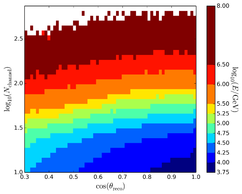
Figure 1.— Median true energy as a function of the cosine of the reconstructed zenith angle $\theta_{\mathrm{reco}}$ and the number of DOMs hit in the event, $N_{\mathrm{channel}}$, from simulation.

It is important to emphasize that scrambling the time of events with a given zenith angle in local detector coordinates is equivalent to randomly modifying the right ascension of the event within the same declination band, with the width of the band determined by the pixelization used. As a result, the residual between the actual arrival direction distribution and the reference maps, determined by independently normalizing each declination band, is sensitive primarily to anisotropy modulations in right ascension (Ahlers et al., 2016). Simulation studies (Santander, 2013) indicate that any structure is effectively reduced to its projection onto right ascension, limiting the sensitivity to the determination of the true anisotropy. The relative intensity of any small-scale features is also underestimated because of the overestimation of the isotropic “floor” for the entire declination band. This distortion is unavoidable, but for the small level of anisotropy and the choice of 24 hours scrambling time in this analysis, the effect is not significant.

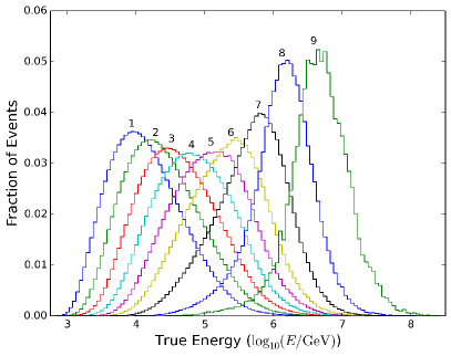
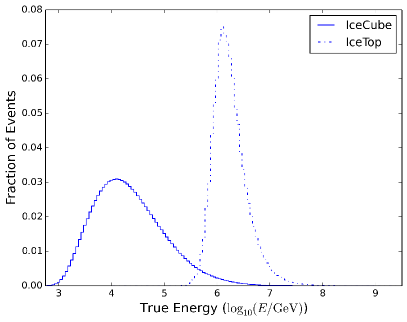
Figure 2.— Left: Fraction of events as a function of the true energy for the nine energy bins used in this analysis, from simulation. The median energy and the 68% central interval for the nine bins are listed in the first row of Tab. 3. The primary cosmic-ray composition and energy spectrum are based on Hörandel (2003). Right: Fraction of events as a function of true energy for the full IceCube (solid line) and IceTop (dashed line) data sets used in this analysis. The IceCube data set includes the data from all nine energy bins plus low energy events not included in the lowest energy bin (see text).

The map of cosmic-ray anisotropy is obtained by calculating the residual between the data map and the reference map. The relative intensity is defined as $\delta I_{i}=(N_{i}-\langle N\rangle_{i})/\langle N\rangle_{i}$, where $N_{i}$ and $\langle N\rangle_{i}$ are the number of observed events and the number of reference events in the $i^{th}$ pixel, respectively. Maps showing the statistical significance of deviations are calculated according to Li & Ma (1983). To study the small-scale anisotropy, the dipole and quadrupole terms of the spherical harmonic functions were fit to the data and then subtracted. All maps undergo a top-hat smoothing procedure in which a single pixel’s value is the sum of all pixels within a given angular distance, or smoothing radius. In the case of this data set, the median angular resolution, as found from simulation, is 3^∘. Therefore, a smoothing of $5^{\circ}$, roughly equivalent to the optimal bin size for point-source searches (Alexandreas et al., 1993), is applied to the maps.

3.2. Separation into Energy Bins

In order to study the anisotropy in cosmic-ray arrival direction as a function of primary energy in IceCube, a similar energy estimation procedure to that of Abbasi et al. (2012) is used. Events are classified using the number of DOMs that detected Cherenkov light, $N_{\mathrm{channel}}$, and the reconstructed zenith angle, $\theta_{\mathrm{reco}}$. $N_{\mathrm{channel}}$ is used as an energy estimator of the muons detected by IceCube. The reconstructed angle $\theta_{\mathrm{reco}}$ is considered because at larger zenith angles muons, and therefore the primary cosmic-ray particles, must have higher energy in order to reach and trigger the buried IceCube experiment. Simulation data are used to determine bands in primary particle energy as a function of $N_{\mathrm{channel}}$ and the cosine of $\theta_{\mathrm{reco}}$, as shown in Fig. 1. The figure shows that for a given $N_{\mathrm{channel}}$, events at larger zenith angles are produced by cosmic-ray particles with higher energy.

Region	Right Ascension (deg)	Declination (deg)	Peak Significance
1a	$142.5_{-2.4}^{+4.9}$	$-49.7_{-3.9}^{+2.3}$	$11.0\sigma$
1b	$110.5_{-3.5}^{+5.3}$	$-55.9_{-2.3}^{+5.4}$	$6.9\sigma$
2	$261.0_{-8.5}^{+3.4}$	$-48.9_{-2.3}^{+4.7}$	$11.4\sigma$
3	$200.4_{-1.4}^{+2.8}$	$-38.7_{-2.3}^{+2.3}$	$10.8\sigma$
4	$327.9_{-16.8}^{+11.9}$	$-74.6_{-4.4}^{+4.4}$	$11.0\sigma$
5	$215.6_{-8.6}^{+18.7}$	$-72.4_{-2.2}^{+5.2}$	$-9.3\sigma$
6	$74.5_{-4.2}^{+4.2}$	$-36.4_{-3.8}^{+5.0}$	$-10.3\sigma$
7a	$317.1_{-2.1}^{+4.2}$	$-38.7_{-1.5}^{+5.2}$	$-7.2\sigma$
7b	$292.5_{-1.4}^{+1.4}$	$-41.0_{-1.6}^{+1.6}$	$-9.6\sigma$
8	$164.7_{-2.9}^{+3.2}$	$-48.1_{-3.9}^{+4.7}$	$-11.9\sigma$
$9^{*}$	$94.1_{-40.9}^{+9.4}$	$-82.0_{-2.2}^{+5.1}$	$-7.9\sigma$
$10^{*}$	$27.4_{-1.4}^{+4.9}$	$-27.3_{-2.0}^{+3.3}$	$10.6\sigma$

Table 2Locations and pre-trial peak significance values for the small-scale structures visible after subtracting the best-fit dipole and quadrupole functions. Errors indicate the positions of the farthest pixels within $1\sigma$ of the peak significance. Regions marked a and b were previously reported as one region. Regions with an asterisk are new to this analysis.

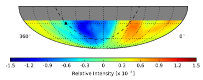
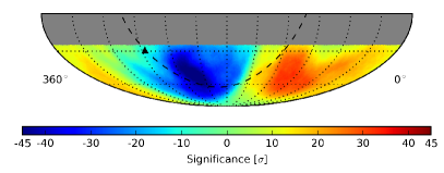
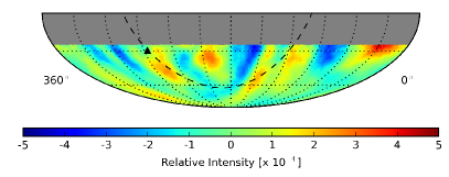
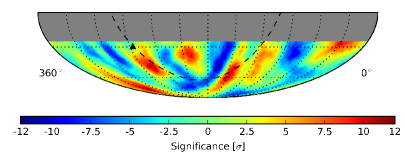
Figure 3.— Relative intensity (left) and pre-trial statistical significance (right) maps shown before (top) and after (bottom) dipole- and quadrupole-subtraction. The maps are in equatorial coordinates and use an angular smoothing radius of $5^{\circ}$. The dashed line indicates the Galactic plane and the triangle indicates the Galactic center.

A B-spline function (see Whitehorn et al. (2013) for a description of the method applied here) in $N_{\mathrm{channel}}$ and $\cos$($\theta_{\mathrm{reco}}$) is used to fit the data in Fig. 1 in order to reduce the errors due to limited simulation data statistics. Events are then separated into nine energy bins with increasing mean primary particle energies ranging from 13 TeV (bin 1) to 5.4 PeV (bin 9). The resolution of this energy assignment depends on the detector configuration and energy band but is on the order of 0.5 in $\log_{10}(E/\mathrm{GeV})$. It is primarily limited by the relatively large fluctuations in the fraction of the total shower energy that is transferred to the muon bundle. The individual colors in Fig. 1 correspond to the different energy bins. The dark blue bin corresponds to events with $\log_{10}(E/\mathrm{GeV})<4.0$. This bin is not used because of the limited zenith range of the events.

The nine data samples created by this method are statistically independent, but as a result of the limited energy resolution, the energy distributions of the events in the bins overlap considerably. To illustrate this, the left panel of Fig. 2 shows the fraction of events as a function of the true primary energy for the nine energy bins, from simulation. The median energy and the 68% central interval for the nine bins are also listed in the first row of Tab. 3. The right panel of Fig. 2 shows the fraction of events as a function of the true primary energy for the entire data set, without energy cuts. Note that this includes all events from the nine energy bins, but also the events in the dark blue bin ($\log_{10}(E/\mathrm{GeV})<4.0$) of Fig. 1 which are not part of the lowest energy bin.

In contrast to IceCube, the IceTop data set at present cannot be split into several energy bins because the total number of events is still too small. For this work, a single high-energy IceTop sample was selected by using all events with $N_{\mathrm{station}}\geq 8$, resulting in a median energy of 1.6 PeV. Fig. 2 (right) shows the fraction of events as a function of the true primary energy for the IceTop data set used in this analysis.

4. Results

4.1. Large- and Small-Scale Structure

Figure 3 shows relative intensity and pre-trial significance sky maps for large- and small-scale structures. All of the maps contain six years of IceCube data at all energies. The energy distribution of these events, i.e., the fraction of events as a function of the true energy, is shown in the right panel of Fig. 2. The maps are top-hat smoothed with a $5^{\circ}$ angular radius. The relative intensity map, shown in the top left plot of Fig. 3, is similar to previously published work based on IC59 data (Abbasi et al., 2011) and shows anisotropy at the $10^{-3}$ level, characterized by a large excess from $30^{\circ}$ to $120^{\circ}$ and a deficit from $150^{\circ}$ to $250^{\circ}$. The corresponding significance of the large-scale structure, shown in the top right plot of Fig. 3, shows the increasingly high statistical significance of the observation. While this large-scale structure dominates the anisotropy, there is also anisotropy on smaller scales. This structure, with a relative intensity on the order of $10^{-4}$, becomes visible after the best-fit dipole and quadrupole are subtracted from the sky map. The lower left panel of Fig. 3 shows the relative intensity of the residual map, and the lower right panel the corresponding significance map. The maps show the presence of cosmic-ray anisotropy at angular scales approaching the angular resolution of IceCube for cosmic-ray primaries.

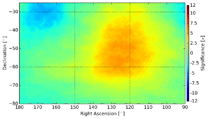
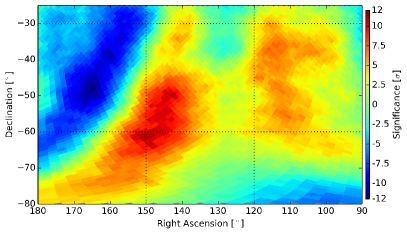
Figure 4.— Significance map in the vicinity of Region 1 (see Tab. 2) as previously published using only data taken with the IC59 configuration (Abbasi et al., 2011) with $20^{\circ}$ smoothing (left) and for the full data set used in this analysis with $5^{\circ}$ smoothing (right). Maps are shown in equatorial coordinates.

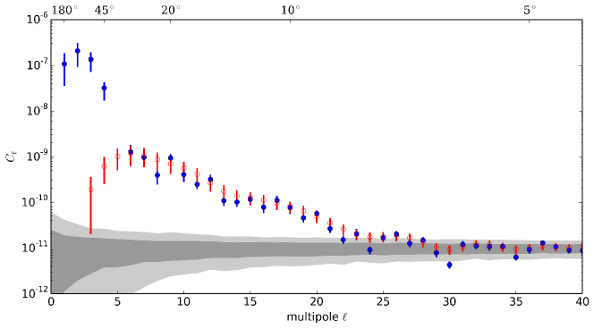
Figure 5.— Angular power spectra for the relative intensity map for six years of IceCube data. Blue and red points show the power spectrum before and after the subtraction of the best-fit dipole and quadrupole terms from the relative intensity map. Error bars are statistical (see the text for a discussion of systematic errors). The gray bands indicate the 68% (dark) and 95% (light) spread in the $C_{\ell}$ for a large sample of isotropic data sets. The power spectrum is calculated using the unsmoothed map.

Table 2 shows the positions and peak significances of excess and deficit regions with a pre-trial significance exceeding $5\sigma$. The regions are numbered to maintain consistency with Abbasi et al. (2011) whenever possible. The significances quoted are pre-trial, and any blind search would have to account for the fact that we search for significant excess or deficit regions anywhere in the roughly $10^{4}$ independent bins of the map. However, all but two of the regions listed in Tab. 2 have been previously reported in the analysis of the IC59 data set. In the new data set, which includes the IC59 data set but is a factor of nine larger, all regions appear with greatly increased significance.

Figure 4 provides an example of how the high-statistics data set reveals more details of the anisotropy. The left plot shows a region of excess using only the IC59 data set with $20^{\circ}$ smoothing applied, as in Abbasi et al. (2011). The same region is shown in the right plot, using the updated data set and $5^{\circ}$ angular smoothing. What previously appeared as one region is now observed as two distinct regions, each at high significance. This difference does not appear to be the result of a time dependence of the small-scale structure, as the same split is visible in the IC59 map with $5^{\circ}$ smoothing but not at high enough significance to be previously reported.

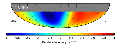
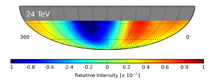
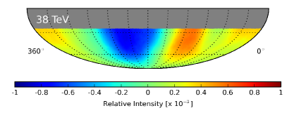
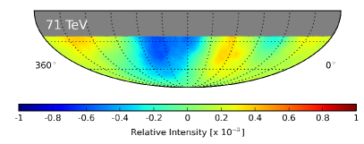
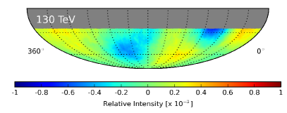
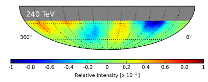
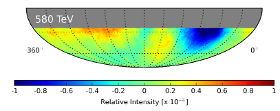
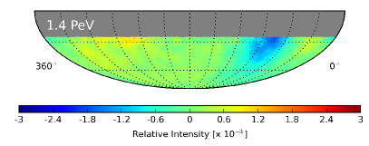
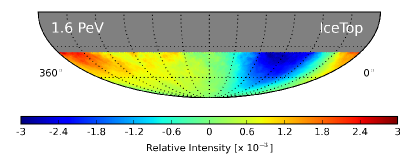
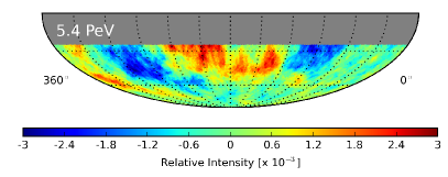
Figure 6.— Relative intensity maps in equatorial coordinates for the energy bins described in Section 3.2. The median energy of the data shown in each map is indicated in the upper left. Maps have been smoothed with a $20^{\circ}$ smoothing radius. The final three maps are shown on a different relative intensity scale. The map at 1.6 PeV in the lower left panel is based on IceTop data. All other maps show IceCube data.

1

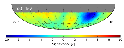
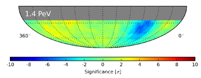
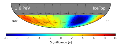
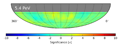
Figure 7.— Significance maps in equatorial coordinates for the four highest energy bins described in Section 3.2. The median energy of the data shown in each map is indicated in the upper left. Maps have been smoothed with a $20^{\circ}$ smoothing radius. The map at 1.6 PeV in the lower left panel is based on IceTop data. All other maps show IceCube data.

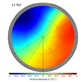
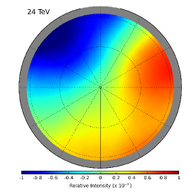
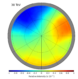
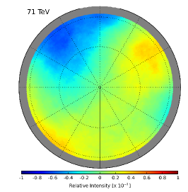
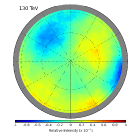
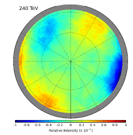
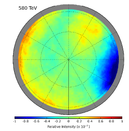
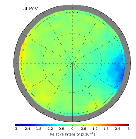
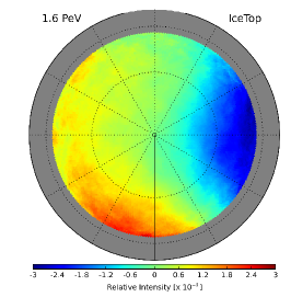
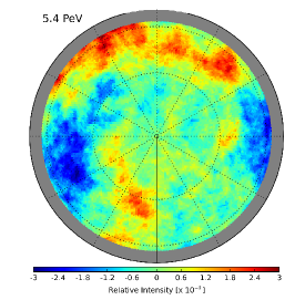
Figure 8.— Relative intensity maps in polar coordinates for the energy bins described in Section 3.2. The median energy of the data shown in each map is indicated in the upper left. Maps have been smoothed with a $20^{\circ}$ smoothing radius. The final three maps are shown on a different relative intensity scale. The 1.6 PeV map is based on IceTop data. All other maps show IceCube data.

The angular power spectrum for the six-year data set is shown in Fig. 5. Similar to previous work, it is calculated using PolSpice (Szapudi et al., 2001; Chon et al., 2004), which corrects for systematic effects introduced by partial-sky coverage. The power spectrum is calculated for the unsmoothed data map and is shown before (blue) and after (red) subtracting the dipole and quadrupole functions from the sky map. The gray bands indicate the 68% and 95% spread in the $C_{\ell}$ for a large number of power spectra for isotropic data sets generated by introducing Poisson fluctuations in the reference skymap. The power spectrum confirms the presence of significant structure up to multipoles $\ell\simeq 20$, corresponding to angular scales of less than $10^{\circ}$.

The error bars on the $C_{\ell}$ shown in Fig. 5 are statistical. We estimate the systematic error caused by the partial-sky coverage by comparing the angular power spectrum before and after subtraction of the best-fit dipole and quadrupole functions. After the subtraction, $C_{1}$ and $C_{2}$ are consistent with zero, as expected. In principle, the two spectra should be identical for all $\ell\geq 3$, but because of the partial-sky coverage, the multipole moments are no longer independent. While PolSpice tries to mitigate the effect of coupling between multipole moments, a significant coupling between the low-$\ell$ modes remains. As a consequence, the subtraction of dipole and quadrupole fits also leads to a strong reduction in the power of the $\ell=3$, $\ell=4$, and $\ell=5$ multipoles. The systematic error on these multipoles is therefore large, as we cannot rule out that the presence of these multipoles is entirely caused by systematic effects. For multipoles $\ell\geq 6$, the distortion is much smaller and the spectra agree within uncertainties. For these moments, the systematic errors on the $C_{\ell}$ are therefore at most of the same order as the statistical errors.

In the unsubtracted power spectrum, the uncertainty in the lower multipole moments causes the $C_{\ell}$ value for $\ell=5$ to be negative — a result of PolSpice’s calculation of the $C_{\ell}$ values through the use of the two-point autocorrelation function. Simulations using artificial sky maps with strong dipole components indicate that this behavior is typical for the weighting and apodization used in this analysis (see Abbasi et al. (2011) for details) and is another indication of the coupling between low-$\ell$ multipoles.

4.2. Energy Dependence of Anisotropy

To study the energy dependence of the cosmic-ray anisotropy, we split the data into the nine energy bins described in Section 3.2. This results in a sequence of maps with increasing median energy, starting from 13 TeV for the lowest-energy bin to 5.3 PeV for the highest-energy bin. The sky maps in relative intensity for all nine energy bins in equatorial coordinates are shown in Fig. 6. In addition to the nine maps based on IceCube data, we also show the IceTop map with its median energy of 1.6 PeV. Because of the reduced statistics in these maps, we have applied a top-hat smoothing procedure with a smoothing radius of $20^{\circ}$ to all, improving the sensitivity to larger structure. Note that the relative intensity scale for these plots is identical for energies up to 580 TeV, where it then switches to a different scale to account for the strong increase in relative intensity. For the IceTop bins with 580 TeV, 1.4 PeV, and 5.4 PeV median energy and for the IceTop data, Fig. 7 shows the sky maps in statistical significance.

The maps clearly indicate a strong energy dependence of the global anisotropy. The large excess from $30^{\circ}$ to $120^{\circ}$ and deficit from $150^{\circ}$ to $250^{\circ}$ that dominate the sky map at lower energies gradually disappear above 50 TeV. Above 100 TeV a change in the morphology is observed. At higher energies, the anisotropy is characterized by a wide relative deficit from $30^{\circ}$ to $120^{\circ}$, with an amplitude increasing with energy up to at least 5 PeV, the highest energies currently accessible to IceCube. To illustrate the phase change, the relative intensity sky maps are shown in polar coordinates in Fig. 8. It is important to note that the time-scrambling method used to calculate the reference map decreases in sensitivity as we approach the polar regions. This effect is clearly visible in Fig. 8, where the relative intensity approaches zero at the pole for each map, but is not indicative of the morphology of the true anisotropy.

Because of the poor energy resolution, it is difficult to accurately determine the energy where the transition in anisotropy occurs and how rapid the transition is. To illustrate the energy dependence of the phase and strength of the anisotropy, we show in Fig. 9 amplitude (left) and phase (right) of the dipole moment as a function of energy. Both values are calculated by fitting the set of harmonic functions with $n\leq 3$ to the projection of the two-dimensional relative intensity map (Fig. 6) in right ascension,

$$\sum_{n=0}^{3}A_{n}\cos[n(\alpha-\phi_{n})]~{},$$ (1)

where $A_{n}$ is the amplitude and $\phi_{n}$ is the phase of the $n^{th}$ harmonic term, respectively. The fit is performed on a projection with a $5^{\circ}$ bin width in right ascension. We fit the one-dimensional projection in right ascension rather than the full sky map because the two-dimensional fit of spherical harmonics to the map is difficult to perform with a limited field of view. As a result of the method we apply to generate the reference map, the sky map will in any case only show the projection of any dipole component, so the one-dimensional fit is sufficient to study the energy dependence of the dominant dipole. The values for the projections in each energy bin are provided in Tab. 3.

R.A.	$\log_{10}(E_{\mathrm{median}}/\mathrm{GeV})$
	$4.12^{+0.62}_{-0.50}$	$4.38^{+0.65}_{-0.54}$	$4.58^{+0.68}_{-0.55}$	$4.85^{+0.73}_{-0.64}$	$5.12^{+0.74}_{-0.72}$	$5.38^{+0.75}_{-0.78}$	$5.77^{+0.60}_{-0.83}$	$6.13^{+0.52}_{-0.63}$	$6.73^{+0.46}_{-0.58}$	$6.21^{+0.36}_{-0.27}$
$350^{\circ}$	3.84	3.56	3.11	1.41	0.89	1.29	0.36	-3.00	6.64	18.29
$330^{\circ}$	2.64	3.45	3.41	2.96	1.81	4.36	1.72	0.90	23.10	15.79
$310^{\circ}$	0.34	1.17	0.78	1.52	2.32	2.77	1.46	8.89	-2.14	8.99
$290^{\circ}$	-3.02	-1.52	-0.16	0.19	1.57	1.26	2.22	1.60	-40.43	6.56
$270^{\circ}$	-4.46	-3.25	-1.72	-0.76	0.64	1.11	1.14	6.56	-2.97	10.44
$250^{\circ}$	-7.11	-6.33	-3.77	-2.63	-2.15	-0.46	2.87	9.04	-8.79	6.02
$230^{\circ}$	-10.30	-10.24	-7.88	-5.59	-4.49	-3.89	2.09	0.85	8.49	11.14
$210^{\circ}$	-9.24	-9.02	-7.24	-5.51	-3.13	-1.71	1.54	5.26	15.01	8.23
$190^{\circ}$	-7.14	-6.74	-5.66	-2.70	-3.07	-0.25	0.46	-0.25	8.10	-0.99
$170^{\circ}$	-5.26	-5.26	-4.27	-3.78	-1.52	2.07	-1.21	0.75	-7.95	2.75
$150^{\circ}$	0.05	0.32	1.54	3.15	2.16	3.93	5.81	1.47	39.23	-1.61
$130^{\circ}$	4.03	3.83	2.82	2.08	1.47	1.07	-1.06	-0.89	-2.84	-11.94
$110^{\circ}$	6.66	7.41	6.62	3.92	2.38	-1.70	-1.46	-4.50	-5.75	-21.35
$90^{\circ}$	6.92	6.09	3.84	1.95	0.84	-0.71	-5.38	-11.09	-11.34	-21.95
$70^{\circ}$	6.06	4.52	1.39	-0.16	-1.53	-7.26	-8.70	-14.24	10.69	-20.22
$50^{\circ}$	5.89	4.18	2.89	0.31	-1.32	-0.74	-2.51	-1.29	-3.25	-17.69
$30^{\circ}$	5.37	4.35	2.23	2.21	3.12	-0.33	-0.05	-0.13	-21.37	0.00
$10^{\circ}$	4.80	3.42	2.08	1.55	-0.14	-0.74	1.92	-1.19	11.77	12.26
$\sigma_{\mathrm{stat}}$	0.18	0.18	0.36	0.66	1.02	1.42	1.49	3.23	14.39	4.48

Table 3Relative intensity ($\times 10^{4}$) projected in right ascension for each energy bin. Right ascension values indicate the center of each bin. Energy values indicate the median true energy for each bin, as estimated by simulation, with error bars containing 68% of the data. The last row gives the mean of the statistical error on the relative intensity values in the column ($\sigma_{stat}$). The separate rightmost column contains data for the IceTop energy bin.

The red data points in Fig. 9 are based on the IceTop data. While the phase agrees well with that of the IceCube data at similar energies, the amplitude of the anisotropy is larger for the IceTop data than for any IceCube energy bin. A possible explanation for the difference could be the different chemical composition of the IceCube and IceTop data sets. Table 4 shows the relative composition of cosmic rays detected in IceCube and IceTop according to simulation, based on a primary cosmic-ray composition according to the model by Hörandel (2003). For IceCube, we list the composition for all nine energy bins. Elements are grouped in four main categories with increasing mass number as described in the caption. The simulation indicates that the data set recorded by IceTop is composed of 34% protons and 12% heavy elements. At a comparable median energy, in the second-highest energy bin, the data set recorded by IceCube is composed of 24% protons and 21% heavy elements. The reason for the discrepancy is the fact that at this median energy, the effective area of IceTop for iron showers is still smaller than for proton showers. Iron primaries start interacting higher in the atmosphere than proton primaries, so iron and proton showers are at different stages of development when reaching the detector altitude. The probability to reach the detector altitude and trigger at low energy is therefore smaller for iron showers than for proton showers. If the anisotropy is predominantly caused by protons, the lighter composition of the IceTop data could lead to a stronger dipole amplitude.

The IceCube and IceTop sky maps also show different structures in other parts of the maps, but as indicated in Fig. 7, most of these structures are not statistically significant, especially near the edge of the field of view. The large structure with a significance of approximately $5\,\sigma$ between $300^{\circ}$ and $360^{\circ}$ in right ascension and $-30^{\circ}$ and $-60^{\circ}$ in declination in the IceTop sky map is also marginally visible in the 1.4 PeV IceCube map, but with a low significance because of the small size of the data set.

$\log_{10}(E_{\mathrm{median}}/\mathrm{GeV})$	H	He	CNO	Fe
4.12	0.74	0.21	0.04	0.01
4.38	0.70	0.23	0.06	0.01
4.58	0.67	0.25	0.07	0.02
4.85	0.61	0.27	0.09	0.03
5.12	0.54	0.28	0.12	0.05
5.38	0.46	0.29	0.16	0.09
5.77	0.35	0.30	0.21	0.14
6.13	0.24	0.28	0.26	0.21
$6.21^{*}$	0.34	0.30	0.24	0.12
6.73	0.17	0.18	0.28	0.37

Table 4Chemical composition of each IceCube energy bin and for IceTop as determined by simulation using a primary chemical composition following Hörandel (2003). Listed is the relative fraction of the composition group in the detected cosmic-ray flux. The composition groups are as follows: H: ${}^{1}\mathrm{H}$, He: ${}^{4}\mathrm{He}$ - ${}^{11}\mathrm{B}$, CNO: ${}^{12}\mathrm{C}$ - ${}^{39}\mathrm{K}$, Fe: ${}^{40}\mathrm{Ca}$ - ${}^{56}\mathrm{Fe}$. The IceTop bin is marked with an asterisk.

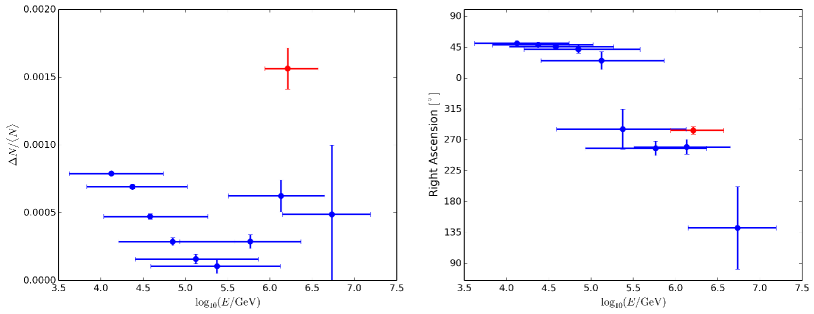
Figure 9.— Amplitude (left) and phase (right) of the dipole moment of the projection of the relative intensity in right ascension for the nine energy bins of IceCube (blue) and for IceTop (red). The projections were fit with the set of harmonic functions (see Eq. 1), but only the dipole is reported here. Data points indicate the median energy of each energy bin, with error bars on the energy showing the 68% central interval.

Figure 10.— Projection of relative intensity for all declinations as a function of right ascension for each configuration of the IceCube detector from IC59 to the fourth year of IC86. The yearly data points are placed side by side in time sequence, and the different right ascension bins are delineated by vertical lines. The shaded areas indicate systematic errors, calculated using the anti-sidereal frame for each year independently.

4.3. Time Dependence of Anisotropy

The data used in this analysis was recorded over a period of six years and therefore also allows for a study of the stability of the anisotropy over this time period. An observed time-modulation of the anisotropy, in particular one that coincides with the 11-year solar cycle, could be evidence for a heliospheric influence on the observations. Time-dependent studies have been performed previously by several experiments, with contradictory results. Milagro reported a steady increase in the amplitude of the large-scale anisotropy over a seven-year time period (2000-2007) (Abdo et al., 2009). However, the Tibet experiment did not observe significant time variation in the large-scale anisotropy between 1999 and 2008 (Amenomori et al., 2010), and the ARGO-YBJ experiment did not observe significant variation in the medium-scale ($10^{\circ}-45^{\circ}$) anisotropy in data covering the period from 2007 to 2012 (Bartoli et al., 2013). Note that the 23rd solar cycle lasted from 1996 June to 2008 January and reached a maximum in March 2000. The current (24th) solar cycle started in January 2008 and reached a maximum in April 2014. The IceCube data set therefore covers the period from minimum to maximum of the current cycle.

Figure 10 shows the one-dimensional projection of the relative intensity in right ascension for each detector configuration used in this analysis, each one corresponding to approximately a year of data (see Tab. 1). The yearly data points are placed side by side in time sequence, and the different right ascension bins are delineated by vertical lines. The shaded regions represent systematic errors determined by calculating the maximum amplitude of the signal in the anti-sidereal time frame (discussed in Section 5). Systematic errors are estimated separately for each detector configuration. The energy distributions for events in the IC59 through IC86-IV data sets are similar and match the distribution shown in the right panel of Fig.2.

Within errors, the large-scale structure is stable over the data taking period considered here. Table 5 shows the $\chi^{2}$ values calculated by comparing each year to the ensemble. The resulting $p$-values are consistent with random fluctuations, indicating there is no time dependence over the period of this study. In addition, no systematic trends with time are detected within the individual right ascension bins in Fig. 10. A study of the stability over a period of twelve years (2000-2012) using data recorded with the AMANDA and IceCube detectors (Aartsen et al., 2013b) with the same method also did not find evidence for a time dependence of the structure.

Configuration	$\chi^{2}$	$N$	$p$-value
IC59	31.42	23	0.11
IC79	16.12	23	0.85
IC86	19.66	23	0.66
IC86-II	15.44	23	0.88
IC86-III	24.27	23	0.39
IC86-IV	18.16	23	0.75

Table 5Results of a $\chi^{2}$ test comparing the relative intensity profile (see Fig. 10) for each year to the collective ensemble. The table provides $\chi^{2}$ values, number of degrees of freedom, $N$, and corresponding $p$-values.

To study the time dependence of the small-scale structure, we analyze the relative intensity of the excess and deficit regions listed in Tab. 2 as a function of time. For the location of the regions, we use the values determined from the full six-year data set. Fig. 11 shows the relative intensity for each detector configuration, i.e., as a function of time, for each region. Also shown is the average value as determined from the analysis of the full six-year data set. The error bars on the data points and the error band on the average indicate statistical uncertainties only, but we list the average flux, including statistical and systematic errors, for each region in the figures. The systematic errors for the individual years have similar values. The relative intensity at the excess and deficit regions of the small-scale structure is constant within errors for the time period covered by this analysis.

As an additional test of the stability of the small-scale map, we subtract the relative intensity sky map of the full six-year data set from the sky map of each individual detector configuration, i.e., of each of the six years of data, and calculate the angular power spectrum of the residual maps. All of them have power spectra that are, within errors, compatible with isotropy, indicating that there are no significant differences between the maps for individual years and the average. The small-scale anisotropy, like the large-scale anisotropy, is constant over the time period covered by this analysis.

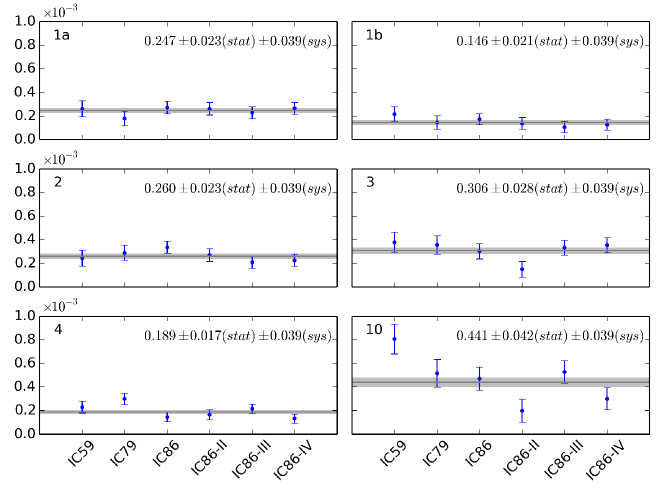
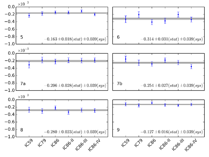
Figure 11.— Relative intensity as a function of detector configuration for the locations of the excess and deficit regions of the small-scale structure listed in Tab. 2. The horizontal lines indicate the six-year average relative intensity. Error bars and bands are statistical, but the relative intensity, including statistical and systematic errors, is given for each region.

5. Systematic Checks

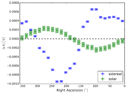
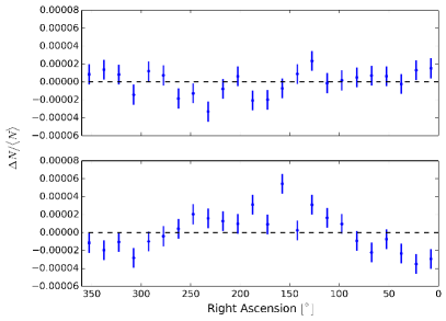
Figure 12.— Projection of relative intensity in right ascension for solar and sidereal time (left), and anti-sidereal (right, top) and extended-sidereal time (right, bottom). Error boxes for the solar and sidereal projection indicate systematic errors. Note that both the anti-sidereal and extended-sidereal frames are non-physical, so “right ascension” has no physical meaning in these frames. For the solar frame, the right ascension axis shows the difference between the right ascension of the event and the right ascension of the Sun.

In Abbasi et al. (2010), several sources of systematic bias are considered, including detector geometry and livetime, nonuniform exposure to different regions of the sky, and seasonal variations in atmospheric conditions. The location of the IceCube detector minimizes the effect of some of these sources; the southern celestial sky is fully visible at all times, and seasonal variations are slow and automatically accounted for in the estimation of the reference map. The checks performed in that previous analysis continue to hold, and the detector livetime has improved on average, as seen in Tab. 1. In this section we expand on one possible source of systematic bias that the increased data set allows us to study in more detail: the possible influence of the solar dipole on the sidereal signal and vice versa.

As the Earth orbits around the Sun, we observe an excess in the relative intensity of cosmic rays in the direction of motion and a corresponding deficit in the direction opposite to the motion. This effect manifests itself as a dipole in the relative intensity when the cosmic-ray arrival directions are plotted using solar time, i.e., in a frame where the position of the Sun is at a fixed location. This solar dipole has been measured previously (Abbasi et al., 2011, 2012) and now serves as a check of the consistency and reliability of the analysis methods used.

Ideally, the solar dipole should not cause any systematic uncertainties in the analysis of cosmic-ray arrival directions in sidereal time, as any signal in solar time averages to zero over a year. In practice, however, seasonal variations in the solar dipole can manifest themselves as an anisotropy in the sidereal time frame and vice versa. In order to study this mutual influence, we consider two nonphysical time scales: anti- and extended-sidereal time.

Solar time has a frequency of 365.24 cycles per year. The sidereal day is roughly four minutes shorter, with a frequency of 366.24 cycles per year. The influence of the solar dipole on the sidereal anisotropy can be estimated from the influence it has on the other side band in frequency space, i.e., on a frame with 364.24 cycles per year. This is the anti-sidereal frame. No physical signal is expected with a frequency of 364.24 cycles per year, so any significant “signal” that appears in the anti-sidereal frame stems from a modulation of the solar frame and is equivalent to the systematic effect of the solar frame on the sidereal frame and therefore on the anisotropy signal. This method can also be used to estimate the effect of the sidereal anisotropy on the solar dipole. In this case, the second side band of the sidereal frame, the extended-sidereal time frame with a frequency of 367.24 cycles per year, can be analyzed. Any significant signal in the extended-sidereal frame is due to seasonal modulations in the sidereal frame and is equivalent to the systematic effect of the sidereal frame on the solar frame.

The projection of the relative intensity in right ascension for the sidereal and solar frames is shown in Fig. 12 (left). For the solar frame, the “right ascension” axis shows the difference between the right ascension of the event and the right ascension of the Sun. In this system, the Sun is located at $0^{\circ}$, so the maximum of relative intensity is at an angle of $270^{\circ}$, in the direction of the Earth’s motion. The solar dipole is well measured with six years of IceCube data. The fit of the projection to a dipole results in an amplitude of $(2.242\pm 0.029)\times 10^{-4}$ and a phase of $(268.00\pm 0.75)^{\circ}$. The $\chi^{2}$-probability of the fit is 0.21 ($\chi^{2}=17.42$ for 23 degrees of freedom). The amplitude of the sidereal anisotropy is larger, but is not well described by a dipole. Statistical errors are shown, but are smaller than the data points due to the high statistics of the data set.

In contrast, Fig. 12 (right) shows the projection of the relative intensity in anti-sidereal and extended-sidereal time. Note that the amplitude of these projections is an order of magnitude smaller than the amplitude of the solar dipole and the sidereal anisotropy, indicating that the effect of the solar on the sidereal frame and vice versa is small. We use the maximum amplitude of the relative intensity in the anti- and extended-sidereal frames as a conservative estimate for the systematic error in the sidereal and solar frame resulting from the other. This amplitude appears as systematic error bars in Fig. 10 and Fig. 12 (left).

6. Summary and Discussion

6.1. Large-Scale Anisotropy

The analysis of 318 billion cosmic-ray events recorded between May 2009 and May 2015 has shown anisotropy in the arrival direction distribution consistent with previously published IceCube results (Abbasi et al., 2011, 2012). The increased statistics of this data set allow for observation of the small-scale structure at a level approaching the angular resolution. The resulting sky map shows separate structures that were not resolved in previous analyses, as well as two new regions, an excess and a deficit, observed with high statistical significance.

In addition, a detailed study of the evolution of the anisotropy as a function of energy in the TeV to PeV range shows a strong dependence of the amplitude and the morphology of the anisotropy on energy. This analysis extends our previous work (Abbasi et al., 2011; Aartsen et al., 2013a) and confirms that the anisotropy changes rather dramatically between 130 TeV and 240 TeV; the phase of a best-fit dipole shifts from around $50^{\circ}$ to $270^{\circ}$ in right ascension. At energies below this shift, the amplitude of the best-fit dipole decreases. Above the shift, it increases again, up to the highest energies currently accessible to IceCube.

The source of the cosmic-ray anisotropy remains unknown. The large-scale anisotropy may be qualitatively explained by homogeneous and isotropic diffusive propagation of cosmic rays in the Galaxy from stochastically distributed sources. Such discrete sources are responsible for a density gradient of cosmic rays, which causes a dipole anisotropy. Numerical studies show that it is possible to find a particular realization of Galactic source distribution that explains the observed non-monotonic energy dependence of the anisotropy amplitude. The change in the phase of the anisotropy between TeV and PeV energies could indicate that the location of the dominant source(s) shifts from the Orion arm to the direction of the Galactic center (Sveshnikova et al., 2013). The observed phase above several hundred TeV coincides with the right ascension of the Galactic center, $\alpha_{GC}=268.4^{\circ}$.

As indicated earlier, the Pierre Auger Observatory has studied the amplitude and phase of the first harmonic modulation in right ascension at EeV energies (Abreu et al., 2011, 2012, 2013; Aab et al., 2015). While the amplitude did not show any significant deviation from isotropy, the phase measurement showed consistent results in adjacent energy bins. This was interpreted as a first indication of anisotropy. At energies below 1 EeV, a phase of $270^{\circ}$ for the first harmonic was found, a result that is consistent with the phase measured at PeV energies by IceCube and IceTop (see Fig. 9). Around 1 EeV, a phase shift occurs, and above 4 EeV, the phase is about $100^{\circ}$. Since this is roughly consistent with the direction towards the Galactic anticenter, the shift might be caused by a transition from a Galactic to an extragalactic origin of cosmic rays. The gap between the IceCube measurements and the measurements by the Pierre Auger Observatory is filled by the KASCADE-Grande experiment. KASCADE-Grande data shows a dipole phase between median energies of 2.7 PeV and 33 PeV which is consistent with the IceCube results at PeV energies and the Auger results below 1 EeV (Chiavassa et al., 2015). For the dipole amplitude, KASCADE-Grande measurements only yield upper limits.

While the interpretation of the dipole phase as an indication of the direction towards the dominant source or sources is tantalizing, simulations of large-scale phase and amplitude resulting from certain source distributions show that for an ensemble of realizations, the mean amplitude is larger than what is observed (Erlykin & Wolfendale, 2006; Blasi & Amato, 2012; Ptuskin, 2012; Pohl & Eichler, 2013; Sveshnikova et al., 2013). It is known that transport of cosmic rays in magnetic fields is anisotropic, even for large magnetic perturbations compared to the regular mean field (Giacalone & Jokipii, 1999; Shalchi, 2009; Tautz, 2009; Desiati & Zweibel, 2014; Shalchi, 2015) and that propagation perpendicular to the local magnetic field direction is slower than in the parallel direction. The possible misalignment between the regular magnetic field and the cosmic-ray density gradient decreases the amplitude of the observed anisotropy. This might explain the observed smaller amplitudes of the anisotropy (Effenberger et al., 2012; Kumar & Eichler, 2014; Mertsch & Funk, 2015), but it also means that the anisotropy does not point in the direction of any particular nearby source.

The fact that the cosmic-ray anisotropy is not a simple dipole, nor well fit solely by lower-multipole terms, suggests that other transport processes might be important as well. For instance, drift diffusion driven by a gradient of cosmic-ray density in the local interstellar medium, producing a bidirectional flow of Galactic cosmic rays, was considered by Amenomori et al. (2007) and Mizoguchi et al. (2009).

6.2. Small-Scale Anisotropy

The small-scale anisotropy may be produced by the interactions of cosmic rays with an isotropically turbulent interstellar magnetic field. Scattering processes with stochastic magnetic instabilities produce perturbations in the arrival direction distribution of an anisotropic distribution of cosmic-ray particles within the scattering mean free path. Such perturbations may be observed as stochastic localized excess or deficit regions (Giacinti & Sigl, 2012; Biermann et al., 2013). The corresponding angular power spectrum can be analytically predicted from Liouville’s theorem (Ahlers, 2014; Ahlers & Mertsch, 2015). The injection scale of interstellar turbulence is on the order of 10 pc within the Galactic arms and 100 pc in the inter-arm regions (Haverkorn et al., 2006). In the cascading processes down to smaller scales, the turbulent eddies become elongated along the magnetic field lines. This anisotropic turbulence makes scattering processes inefficient. The scattering mean free path can be larger than the turbulence injection scale, so particles basically stream along magnetic field lines with small cross-field line transport (Yan & Lazarian, 2008; Lazarian & Yan, 2014).

Besides the cascading interstellar magnetic field turbulence down to the damping scale (typically on the order of 0.1 pc), there are other sources of magnetic perturbations on smaller scales. The closest to Earth is represented by the heliosphere, formed by the interaction between the solar wind and the interstellar flow. It is about 600 astronomical units (AU) wide, and it could extend several thousand AU downstream of the interstellar wind (Pogorelov et al., 2009). Globally, the heliosphere constitutes a perturbation in the 3 $\mu$G local interstellar magnetic field with an injection scale comparable to the $\sim$ 10 TeV proton gyroradius (0.003 pc, or 620 AU). It is therefore reasonable that the local interstellar magnetic field draping around the heliosphere might be a significant source of resonant scattering, capable of redistributing the arrival directions of TeV cosmic-ray particles.

6.3. Time Dependence

A study of the time dependence of the large- and small-scale structure over the six-year period covered by this analysis reveals no significant change with time. This result is consistent with previous studies in the Northern and Southern Hemispheres (Bartoli et al., 2013; Amenomori et al., 2010; Aartsen et al., 2013b), but inconsistent with others (Nagashima et al., 1998; Abdo et al., 2008).

We do not expect time variations due to interstellar magnetic field effects, so the non-observation of time variations does not constrain any astrophysical scenarios that could explain the cosmic-ray anisotropy. However, time variations are expected to arise from local phenomena within the heliosphere. At TeV energies, we are not sensitive to the effects of the solar wind and to the direct effects of the solar cycles. Such direct effects, caused by the modulation of the solar wind average strength and its interaction with the cosmic rays, are only detectable at energies below 30 GeV. Modulations in the cosmic-ray spectrum below 30 GeV arising from the 11-year solar cycle have been observed by other experiments (Potgieter et al., 2014, 2015; Adriani et al., 2015).

On the other hand, there could be an indirect effect of the solar cycles on higher energy cosmic rays. This might arise from the fact that the reversing in the solar magnetic field polarity every 11 years produces vast regions of magnetized plasma pushed away from the Sun straight into the heliospheric tail by the solar wind. In such regions the magnetic field is expected to have a coherent polarity (Pogorelov et al., 2009). Subsequent 11-year solar cycles, therefore, produce a series of reversing uni-polar magnetic field regions that are pushed towards the heliotail. Each region is approximately 200 to 300 AU wide, roughly the proton gyroradius at TeV energies in typical Galactic magnetic fields. Cosmic rays, especially with high $Z$, might be affected by these magnetized regions, in particular those produced in the previous solar cycle and just past the solar system towards the heliotail (Lazarian & Desiati, 2010; Desiati & Lazarian, 2012, 2013). We should observe an 11-year modulation, although not necessarily in sync with the current solar cycle. However, based on current observations, such effects may be very small, possibly smaller than $10^{-5}$ in relative intensity, and they might only be detectable towards the general direction of the heliotail.

Annual modulations may also be expected from the fact that in December, Earth is slightly closer to the heliotail than in June. However, the variability in relative intensity is also expected to be of the order of $10^{-5}$ or less and cannot be detected or excluded with IceCube data.

6.4. Outlook

The PeV energy region is not only significant for the energy-dependent cosmic-ray anisotropy; it is also a region where the cosmic-ray energy spectrum shows noticeable fine structure and the chemical composition of the cosmic-ray flux changes (see for example Aartsen et al. (2013c)). In the future, we will focus on a detailed study of possible connections between the arrival direction anisotropy and the energy spectrum and chemical composition of the cosmic-ray flux. The IceTop air shower array has an energy resolution better than 0.1 in $\log_{10}(E/\mathrm{GeV})$ (Abbasi et al., 2013a). IceTop data can thus be used to compare the energy spectrum in regions of excess or deficit flux to the isotropic spectrum. At TeV energies, this type of analysis already showed that the spectrum in excess regions is harder than the overall energy spectrum (Abdo et al., 2008; Bartoli et al., 2013; Abeysekara et al., 2014). With IceTop data, we can search for similar effects at PeV energies. IceTop also has some sensitivity to the chemical composition of the cosmic-ray flux. A study of composition-dependent parameters as a function of sky location could reveal correlations between the anisotropy and the composition of the cosmic-ray flux. In addition, future data will help to extend the IceCube/IceTop measurements to higher energies where they can be compared with results from the KASCADE-Grande experiment in the Northern Hemisphere.

With new cosmic-ray data of unprecedented quantity and quality now available from a number of experiments, the challenge for any theory of cosmic-ray origin and propagation is to explain simultaneously the fine structure of the cosmic-ray energy spectrum, the chemical composition of the cosmic-ray flux, and the amplitude and phase of the anisotropy over a wide energy range from TeV to EeV energies.

References

- Aab et al. (2015) Aab, A., Abreu, P., Aglietta, M., et al. 2015, Proc. 34th Int. Cosmic Ray Conference, The Hague, Netherlands
- Aartsen et al. (2013a) Aartsen, M. G., Abbasi, R., Abdou, Y., et al. 2013a, ApJ, 765, 55
- Aartsen et al. (2013b) —. 2013b, Proc. 33rd Int. Cosmic Ray Conference, Rio de Janeiro, Brasil
- Aartsen et al. (2013c) —. 2013c, Phys. Rev. D, 88, 042004
- Aartsen et al. (2014) Aartsen, M. G., Abbasi, R., Ackermann, M., et al. 2014, Journal of Instrumentation, 9, P03009
- Abbasi et al. (2010) Abbasi, R., Abdou, Y., Abu-Zayyad, T., et al. 2010, ApJ, 718, L194
- Abbasi et al. (2011) —. 2011, ApJ, 740, 16
- Abbasi et al. (2012) —. 2012, ApJ, 746, 33
- Abbasi et al. (2013a) Abbasi, R., Abdou, Y., Ackermann, M., et al. 2013a, Nucl. Instr. Meth. Phys. Res. A, 700, 188
- Abbasi et al. (2013b) —. 2013b, Phys. Rev. D, 87, 012005
- Abbasi et al. (2014) Abbasi, R., Abe, M., Abu-Zayyad, T., et al. 2014, ApJ, 790, L21
- Abdo et al. (2008) Abdo, A., Allen, B., Aune, T., et al. 2008, Phys. Rev. Lett., 101, 221101
- Abdo et al. (2009) —. 2009, ApJ, 698, 2121
- Abeysekara et al. (2014) Abeysekara, A., Alfaro, R., Alvarez, C., et al. 2014, ApJ, 796, 108
- Abreu et al. (2011) Abreu, P., Aglietta, M., Ahn, E.-J., et al. 2011, Astropart. Phys., 34, 627
- Abreu et al. (2012) —. 2012, ApJS, 203, 34
- Abreu et al. (2013) Abreu, P., Aglietta, M., Ahlers, M., et al. 2013, ApJ, 762, L13
- Achterberg et al. (2006) Achterberg, A., Ackermann, M., Adams, J., et al. 2006, Astropart. Phys., 26, 155
- Adriani et al. (2015) Adriani, O., Barbarino, G., Bazilevskaya, G., et al. 2015, ApJ, 810, 142
- Aglietta et al. (2009) Aglietta, M., Alekseenko, V., Alessandro, B., et al. 2009, ApJ, 692, L130
- Ahlers (2014) Ahlers, M. 2014, Phys. Rev. Lett., 112, 021101
- Ahlers & Mertsch (2015) Ahlers, M., & Mertsch, P. 2015, ApJ, 815, L2
- Ahlers et al. (2016) Ahlers, M., BenZvi, S., Desiati, P., et al. 2016, ApJ, 823, 10
- Ahn et al. (2009) Ahn, E.-J., Engel, R., Gaisser, T., Lipari, P., & Stanev, T. 2009, Phys. Rev. D, 80, 094003
- Alexandreas et al. (1993) Alexandreas, D., Berley, D., Biller, S., et al. 1993, Nucl. Instr. Meth. Phys. Res. A, 328, 570
- Amenomori et al. (2005) Amenomori, M., Ayabe, S., Cui, S., et al. 2005, ApJ, 626, L29
- Amenomori et al. (2006) Amenomori, M., Ayabe, S., Bi, X. J., et al. 2006, Science, 314, 439
- Amenomori et al. (2007) Amenomori, M., Ayabe, S., Bi, X. J., et al. 2007, AIP Conf. Proc. 932, 283
- Amenomori et al. (2010) Amenomori, M., Bi, X. J., Chen, D., et al. 2010, ApJ, 711, 119
- Amenomori et al. (2015) —. 2015, Proc. 34th Int. Cosmic Ray Conference, The Hague, Netherlands
- Barrett et al. (1952) Barrett, P. H., Bollinger, L. M., Cocconi, G., Eisenberg, Y., & Greisen, K. 1952, Rev. Mod. Phys. 24, 133
- Bartoli et al. (2013) Bartoli, B., Bernardini, P., Bi, X. J., et al. 2013, Phys. Rev. D, 88, 082001
- Bartoli et al. (2015) —. 2015, ApJ, 809, 90
- Biermann et al. (2013) Biermann, P. L., Becker Tjus, J., Seo, E.-S., & Mandelartz, M. 2013, ApJ, 768, 124
- Blasi & Amato (2012) Blasi, P., & Amato, E. 2012, J. Cosmology Astropart. Phys, 1, 11
- Chiavassa et al. (2014) Chiavassa, A., Apel, W. D., Arteaga-Velázquez, J. C., et al. 2014, Journal of Physics Conference Series, 531, 012001
- Chiavassa et al. (2015) —. 2015, Proc. 34th Int. Cosmic Ray Conference, The Hague, Netherlands
- Chon et al. (2004) Chon, G., Challinor, A., Prunet, S., Hivon, E., & Szapudi, I. 2004, MNRAS, 350, 914
- De Jong et al. (2011) De Jong, J., et al. 2011, Proc. 32nd Int. Cosmic Ray Conference, Beijing, China, 4, 46
- Desiati (2011) Desiati, P. 2011, Proc. 32nd Int. Cosmic Ray Conference, Beijing, China, 1, 78
- Desiati & Lazarian (2012) Desiati, P., & Lazarian, A. 2012, Nonlinear Processes in Geophysics, 19, 351
- Desiati & Lazarian (2013) —. 2013, ApJ, 762, 44
- Desiati & Zweibel (2014) Desiati, P., & Zweibel, E. G. 2014, ApJ, 791, 51
- Duperier (1949) Duperier, A. 1949, Proc. Phys. Soc. A 62, 359
- Duperier (1951) —. 1951, J. Atmos. Terr. Phys. 1, 296
- Effenberger et al. (2012) Effenberger, F., Fichtner, H., Scherer, K., & Büsching, I. 2012, A&A, 547, A120
- Erlykin & Wolfendale (2006) Erlykin, A. D., & Wolfendale, A. W. 2006, Astropart. Phys., 25, 183
- Giacalone & Jokipii (1999) Giacalone, J., & Jokipii, J. R. 1999, ApJ, 520, 204
- Giacinti & Sigl (2012) Giacinti, G., & Sigl, G. 2012, Phys. Rev. Lett., 109, 071101
- Górski et al. (2005) Górski, K. M., Hivon, E., Banday, A. J., et al. 2005, ApJ, 622, 759
- Guillian et al. (2007) Guillian, G., Hosaka, J., Ishihara, K., et al. 2007, Phys. Rev. D, 75, 062003
- Hall et al. (1999) Hall, D. L., Munakata, K., Yasue, S., et al. 1999, J. Geophys. Res., 104, 6737
- Haverkorn et al. (2006) Haverkorn, M., Gaensler, B. M., Brown, J. C., et al. 2006, ApJ, 637, L33
- Heck et al. (1998) Heck, D., Knapp, J., Capdevielle, J. N., Schatz, G., & Thouw, T. 1998, CORSIKA: A Monte Carlo Code to Simulate Extensive Air Showers, Tech. Rep. FZKA-6019
- Hörandel (2003) Hörandel, J. R. 2003, Astropart. Phys., 19, 193
- Kelley et al. (2014) Kelley, J., et al. 2014, AIP Conference Proceedings, 1630, 154
- Kumar & Eichler (2014) Kumar, R., & Eichler, D. 2014, ApJ, 785, 129
- Lazarian & Desiati (2010) Lazarian, A., & Desiati, P. 2010, ApJ, 722, 188
- Lazarian & Yan (2014) Lazarian, A., & Yan, H. 2014, ApJ, 784, 38
- Li & Ma (1983) Li, T.-P., & Ma, Y.-Q. 1983, ApJ, 272, 317
- Mertsch & Funk (2015) Mertsch, P., & Funk, S. 2015, Phys. Rev. Lett., 114, 021101
- Mizoguchi et al. (2009) Mizoguchi, Y., Munakata, K., Takita, M., & Kota, J. 2009, Proc. 31st Int. Cosmic Ray Conference, Lodz, Poland
- Munakata et al. (2010) Munakata, K., Mizoguchi, Y., Kato, C., et al. 2010, ApJ, 712, 1100
- Nagashima et al. (1998) Nagashima, K., Fujimoto, K., & Jacklyn, R. M. 1998, J. Geophys. Res., 103, 17429
- Oshima et al. (2011) Oshima, A., Antia, H., Dugad, S., et al. 2011, Proc. 32nd Int. Cosmic Ray Conference, Beijing, China, 1, 109
- Pogorelov et al. (2009) Pogorelov, N. V., Borovikov, S. N., Zank, G. P., & Ogino, T. 2009, ApJ, 696, 1478
- Pohl & Eichler (2013) Pohl, M., & Eichler, D. 2013, ApJ, 766, 4
- Potgieter et al. (2014) Potgieter, M. S., Vos, E. E., Boezio, M., et al. 2014, Solar Physics, 289, 391
- Potgieter et al. (2015) Potgieter, M. S., Vos, E. E., Munini, R., Boezio, M., & Felice, V. D. 2015, ApJ, 810, 141
- Ptuskin (2012) Ptuskin, V. 2012, Astropart. Phys., 39, 44
- Santander (2013) Santander, M. 2013, PhD Thesis, University of Wisconsin-Madison
- Shalchi (2009) Shalchi, A. 2009, Nonlinear Cosmic Ray Diffusion Theories, Vol. 362 (Springer-Verlag Berlin Heidelberg)
- Shalchi (2015) —. 2015, Physics of Plasmas, 22, 010704
- Sveshnikova et al. (2013) Sveshnikova, L. G., Strelnikova, O. N., & Ptuskin, V. S. 2013, Astropart. Phys., 50, 33
- Szapudi et al. (2001) Szapudi, I., Prunet, S., Pogosyan, D., Szalay, A. S., & Bond, J. R. 2001, ApJ, 548, L115
- Tautz (2009) Tautz, R. C. 2009, ApJ, 703, 1294
- Trefall (1955) Trefall, H., 1955, Proc. Phys. Soc. A 68, 625
- Tilav et al. (2010) Tilav, S., Desiati, P., Kuwabara, T., et al. 2010, Proc. 31st Int. Cosmic Ray Conference, Lodz, Poland
- Whitehorn et al. (2013) Whitehorn, N., van Santen, J., & Lafebre, S. 2013, Comput. Phys. Commun., 184, 2214
- Yan & Lazarian (2008) Yan, H., & Lazarian, A. 2008, ApJ, 673, 942