The Accretion Disk Wind in the Black Hole GRS 1915+105

Abstract

We report on a 120 ks Chandra/HETG spectrum of the black hole GRS 1915$+$105. The observation was made during an extended and bright soft state in June, 2015. An extremely rich disk wind absorption spectrum is detected, similar to that observed at lower sensitivity in 2007. The very high resolution of the third-order spectrum reveals four components to the disk wind in the Fe K band alone; the fastest has a blue-shift of $v=0.03c$. Broadened re-emission from the wind is also detected in the first-order spectrum, giving rise to clear accretion disk P Cygni profiles. Dynamical modeling of the re-emission spectrum gives wind launching radii of $r\simeq 10^{2-4}~{}{\rm GM/c^{2}}$. Wind density values of $n\simeq 10^{13-16}~{}{\rm cm}^{-3}$ are then required by the ionization parameter formalism. The small launching radii, high density values, and inferred high mass outflow rates signal a role for magnetic driving. With simple, reasonable assumptions, the wind properties constrain the magnitude of the emergent magnetic field to be $B\simeq 10^{3-4}$ Gauss if the wind is driven via magnetohydrodynamic (MHD) pressure from within the disk, and $B\simeq 10^{4-5}$ Gauss if the wind is driven by magnetocentrifugal acceleration. The MHD estimates are below upper limits predicted by the canonical $\alpha$-disk model (Shakura & Sunyaev 1973). We discuss these results in terms of fundamental disk physics and black hole accretion modes.

1. Introduction

Disk accretion onto stellar-mass black holes at high Eddington fractions is dominated by thermal emission from an accretion disk. This blackbody-like emission can be characterized extremely well with just two parameters: flux, and color temperature. This simplicity enables efficient traces of disk temperature across orders of magnitude in flux (e.g. Reynolds & Miller 2013), but it hides the underlying physics that mediate the accretion process.

The magneto-rotational instability (MRI; Balbus & Hawley 1991) appears to supply the degree of effective viscosity required to drive disk accretion. Alternatively, gas might escape along poloidal magnetic field lines, transferring angular momentum and allowing mass transfer through the disk (e.g., Blandford & Payne 1982). Accretion in FU Ori and T Tauri systems suggests that these mechanisms might operate concurrently: thermal continuum emission signals a viscous disk, but the profiles observed in line spectra signal a rotating disk wind (e.g., Calvet, Kenyon, & Hartmann 1993). If young stellar disks are any guide, line spectra and winds may hold the key to understanding disks around black holes.

Miller et al. (2015) recently examined the richest disk winds found in Chandra/HETG spectra of the stellar-mass black holes 4U 1630$-$472, H 1743$-$322, GRO J1655$-$40, and GRS 1915$+$105. The observations were obtained in the disk–dominated “high/soft” or “thermal dominant” state (see, e.g., Remillard & McClintock 2006). The Fe K band was found to require 2–3 velocity/ionization components when fit with new, self-consistent XSTAR photoionization models. The spectra also require re-emission from the dense absorbing gas, and the emission is broadened by a degree that is loosely consistent with Keplerian orbital motion at the photoionization radius. This provides a means of estimating wind launching radii, densities, outflow rates, kinetic power, and driving mechanisms.

The observation of GRS 1915$+$105 treated in Miller et al. (2015) was obtained during an extended soft state in 2007 (also see Ueda et al. 2009, Neilsen & Lee 2009). In the spring of 2015, GRS 1915$+$105 was observed to be in a long decline in the SWIFT/BAT (15–50 keV). The source flux eventually became consistent with zero in single visits, indicating that GRS 1915$+$105 had again locked into a steady soft state. We therefore triggered an approved Chandra target of opportunity (TOO) observation of GRS 1915$+$105.

2. Observations and Reduction

GRS 1915$+$105 was observed for 120 ks starting on 2015 June 9 at 15:30:59 UT (”obsid” 16711), using the HETGS. Owing to the high flux level expected in the Chandra band, the ACIS-S array was read-out in ”continuous clocking” mode to prevent photon pile-up, reducing the nominal frame time to just 2.85 ms. A 100-column ”gray” filter was applied across the full height of the S3 chip, windowing the zeroth-order aimpoint. Within this window, one in 10 events was telemetered; this enables the wavelength grid to be reconstructed while preserving telemetry.

CIAO version 4.7 and the associated current calibration files were used to generate spectral files and responses. The tool ”add_grating_orders” was used to combine opposing spectra from the first and third orders. Redistribution matrices were created using the tool ”mkgrmf” and the ancillary responses were created using ”mkgarf”.

The Fe K band traces the mostly highly ionized gas, likely originating closest to the black hole. Following Miller et al. (2015), we proceed to only analyze the combined third-order HEG spectrum in the 5–8 keV band (above 8 keV, order sorting becomes difficult and stray flux enters the extraction region), and the combined first-order HEG spectrum over the 5–10 keV band.

3. Analysis and Results

Models were fit to the data using XSPEC version 12.8.2 (Arnaud 1996). In all of the fits, ”Churazov” weighting (Churazov et al. 1996) was adopted. All of the errors reported in this work are $1\sigma$ confidence intervals.

An equivalent neutral hydrogen column density of $N_{\rm ISM}=4.0\times 10^{22}~{}{\rm cm}^{-2}$ was assumed in all fits and modeled using “tbabs” (Wilms et al. 2000). Fits to the first-order spectrum confirmed that the continuum can be well described with disk blackbody (Mitsuda et al. 1984) and power-law components. The $kT\simeq 1.6$ keV thermal emission dominates over the steep ($\Gamma\simeq 2.8$) power-law (see Table 1). This characterization of the first-order spectrum gives an unabsorbed flux of $F\simeq 4.1\times 10^{-8}~{}{\rm erg}~{}{\rm cm}^{-2}~{}{\rm s}^{-1}$ in the 0.5–30.0 keV band, corresponding to a luminosity of $L\simeq 3.7\times 10^{38}~{}{\rm erg}~{}{\rm s}^{-1}$ for $d=8.6$ kpc (Reid et al. 2014).

In order to characterize the the wind, we generated a grid of photoionized line spectra using XSTAR version 2.2.1bo8 (see, e.g., Kallman et al. 2009). This (newest) version of the code includes the effects of resonant scattering when calculating emission spectra, in addition to recombination, fluorescence, and collisional ionization. A blackbody input spectrum with $kT=1.6$ keV and $L=3.7\times 10^{38}~{}{\rm erg}~{}{\rm s}^{-1}$ was assumed. Following Miller et al. (2015), a turbulent velocity of $300~{}{\rm km}~{}{\rm s}^{-1}$, solar abundances (except for iron, fixed at twice the solar value as per Lee et al. 2002), a covering factor of $\Omega/4\pi=0.5$, and a gas density of $n=10^{14}~{}{\rm cm}^{-3}$ were assumed. Via the ”xstar2xspec” function, 400 photoionization models were created, spanning a range of $6.0\times 10^{21}~{}{\rm cm}^{-2}\leq N\leq 6.0\times 10^{23}$, and $3.0\leq{\rm log}(\xi)\leq 6.0$. The resolution of the models was set to give 100,000 spectral bins.

Photoionized absorption was included in the overall model as a multiplicative component acting upon the continuum. It was characterized in terms of a column density, ionization parameter, and velocity shift (${\rm N}_{H,wind}$, $\xi=L/nr^{2}$, and $v/c$). Self-consistency demands an additive re-emission component for each absorption component. The column density and ionization parameter were linked between the absorption and re-emission components in each zone. The emission component carries a flux normalization, given by $K=(\Omega/4\pi)~{}L_{38}/d_{kpc}^{2}$ (where $L_{38}$ is the luminosity in units of $10^{38}~{}{\rm erg}~{}{\rm s}^{-1}$ and $d_{kpc}$ is the distance in units of kpc). Normalization values were restricted to the 0.1–10.0 range. The re-emission spectra are consistent with a gas at zero velocity shift, per emission from a broad range of azimuth in a cylindrical geometry. Emission velocity shifts were then fixed at zero.

The re-emission is broadened, and is expected to have a non-Gaussian shape if it originates from several hundred or several thousand radii. We therefore convolved each re-emission component with the “rdblur” function (Fabian et al. 1989). This Schwarzschild function differs negligibly from the anticipated (see, e.g., McClintock et al. 2006, Miller et al. 2013) near-maximal Kerr potential far from the black hole, and its range extends to the launching radii whereas newer Kerr blurring functions do not. The inclination was jointly determined between all zones (restricted to the $60^{\circ}\leq\theta\leq 80^{\circ}$ range). Tests revealed that a constant density emissivity profile ($r^{-2}$) gave the best fits, with the outer radius fixed at a multiple of the inner radius for all zones. A value of 5.0 gave the lowest fit statistic ($R_{out}=5.0\times R_{in}$), and values reported in Table 1 reflect fits made with this scheme. Last, a Gaussian emission feature with an energy constrained to lie in the 6.40–6.43 keV range (Fe I-XVII) was included to account for any distant, low-ionization emission.

Initial fits were made to the first and third-order spectra separately. A model with three zones is able to reproduce the lines in the third-order spectrum below 7 keV, and even an H-like absorption doublet blue-shifted by approximately 0.01 c, up to 7.05 keV. However, a weak H-like doublet is apparent at approximately 7.2 keV. We therefore included a fourth zone in fits to the third-order spectrum, measuring a blue-shift of $v=0.0305(4)~{}c$.

We next made joint fits to the first-order and third-order spectra. The continuum in the first-order spectrum is robust and reported in Table 1, but the continuum in the third-order is affected by stray continuum flux, so the continuum parameters and column densities are not linked between the two spectra. The first-order spectrum is generally more sensitive and the parameters of the third-order wind model were tied to those for the first-order spectrum, with the exception of the third and fourth zones, which carry higher velocity shifts. For those zones, the velocity is determined by the third-order spectrum.

The best-fit model is detailed in Table 1. The fits are shown in Figures 1 and 2. Figure 3 illustrates that the re-emission spectrum is broadened. Last, Figure 4 compares the 2007 and 2015 spectra of the high/soft state in GRS 1915$+$105. Overall, a good fit is achieved, with $\chi^{2}/\nu=1951.2/1572=1.241$. Each zone is required by the data, as measured by the F-statistic. The best two-zone model is an enormous ($>>8\sigma$) improvement over the best single-zone model. The best three-zone model is a $5\sigma$ improvement over any fit with just two zones. The addition of the fourth zone is a $3\sigma$ improvement over any three-zone model. Re-emission from Zone 3 is not highly broadened, suggesting a more distant origin. The re-emission from Zone 4 is not well-constrained, and was fixed at a representative value of $K=0.5$. In general, the re-emission normalizations should be regarded as relative scaling factors, since they are partially affected by small continuum disparities between the first and third-order spectra.

The slower components of the wind (Zones 1 and 2 in Table 1) have lower ionizations and higher densities; in contrast, the faster components (Zones 3 and 4 in Table 1) have higher ionizations, and lower densities. This may be consistent with acceleration within the absorbing region. However, the fastest component - Zone 4 - appears to originate at small radii. The wind is likely inconsistent with a homogeneous flow with uniform acceleration, but it may be consistent with a complex flow with multiple stream lines.

Table 1 also gives estimates of the gas density, mass outflow rate, kinetic power, and filling factor in each wind zone. The gas density was obtained through the ionization parameter ($\xi=L/nr^{2}$), utilizing the radius implied by the broadening of the re-emission. The mass outflow rate is estimated without assuming a density by utilizing $L/\xi=nr^{2}$, giving $\dot{M}_{wind}=\Omega\mu m_{p}v(L/\xi)$. The kinetic power is then just $L_{kin}=0.5\dot{M}_{wind}v^{2}$. It is notable that the outflow rate is comparable to the accretion rate in the inner disk in Zones 2, 3, and 4. Summing all zones, the kinetic power of the wind is nominally about 0.1% of the radiative power. The thickness of each wind zone can be estimated via $\Delta r=N/n$, and the volume filling factor is then given by $f=\Delta r/r$. Table 1 gives estimates of $f$ for each zone. Depending on the geometry, it may or may not be appropriate to multiply the mass outflow rates and kinetic power by $f$, reducing both quantities. The best fits are obtained when $\Delta r/r=5$ in the blurring function; this may indicate that the filling factor is not very small.

Radiative line driving is only effective for ${\rm log}(\xi)\leq 3$ (Proga 2003); the wind cannot be driven in this manner. Thermal driving is effective outside of the Comptonization radius, $R_{C}=10^{10}\times(M_{BH}/(M_{\odot})/T_{C,8}~{}{\rm cm}$ (where $T_{C,8}$ is the Compton temperature in units of $10^{8}$ K; Begelman et al. 1983). Other work suggests that winds can be driven from 0.1 $R_{C}$ (Woods et al. 1996; also see Proga & Kallman 2002). Approximating the Compton temperature with the disk temperature (reasonable under equilibrium conditions), $R_{C}\simeq 5\times 10^{11}$ cm, or $3.3\times 10^{5}~{}{\rm GM/c^{2}}$. Thus, $R_{C}$ is 2–3 orders of magnitude larger than implied by the broadening of the re-emission spectra of Zones 1, 2, and 4 (see Table 1). The wind densities and outflow rates also exceed estimates from thermal driving models, though such models are evolving (e.g., Higginbottom & Proga 2015). Emission line broadening might arise via turbulent motions in thermal winds (e.g., Sim et al. 2010). However, this would lead to similar line widths in emission and absorption, whereas the emission lines are much broader than the absorption lines in our best-fit model (see Figure 3).

If the wind is driven by MHD pressure (e.g., Proga et al. 2003), the magnetic pressure must equal or exceed the gas pressure in the wind, meaning that $B^{2}/8\pi=2nkT$, or $B=\sqrt{16\pi nkT}$. If magnetocentrifugal driving (Blandford & Payne 1982) dominates, the magnetic field pressure must equal or exceed the ram pressure of the wind (else the poloidal field geometry will break down), giving $B^{2}/8\pi=0.5\rho v_{tot}^{2}$, or $B=\sqrt{4\pi\mu m_{p}nv_{tot}^{2}}$ (where $v_{tot}$ includes radial and azimuthal velocities). We ran new XSTAR models assuming the derived densities to ascertain the temperature within the wind; these temperatures and the magnetic field magnitudes are listed in Table 1. Using equation 2.19 in Shakura & Sunyaev (1973), limits on the magnetic field strength expected in the $\alpha$-disk prescription were calculated; these are also listed in Table 1.

4. Discussion and Conclusions

We have obtained a sensitive Chandra/HETGS observation of the black hole GRS 1915$+$105, in an extended soft state. The spectrum shows strong absorption lines in the Fe K band, and weaker, broadened emission lines, together creating accretion disk P Cygni profiles (see Figures 1–4). Four distinct wind zones are detected in fits to the first and third-order spectra; the fastest has a blue shift of $v=0.03c$. The broadening of the re-emission components of the wind permits measurements of its launching radius ($R\simeq 10^{2-4}~{}{\rm GM/c^{2}}$), which in turn allow for estimates of the wind density ($n\simeq 10^{13-16}~{}{\rm cm}^{-3}$) and other parameters. The wind is likely driven by magnetic processes, connecting the wind to fundamental aspects of disk accretion, including momentum and mass transfer.

Though luminosities can be difficult to estimate even for X-ray binaries, we observed GRS 1915$+$105 at an apparent luminosity of $L=0.28~{}L_{Edd}$, assuming the most recent estimates of its distance and mass. This is significant because simulations suggest that standard thin accretion disks operate at this Eddington fraction (e.g., Shafee et al. 2008, Reynolds & Fabian 2008). Simulations find that winds might be Compton-thick very close to the disk, but do not remain so as the gas moves upward and outward (Chakravorty et al. 2016). It is possible but unlikely that a Compton-thick, super-Eddington flow was observed in GRS 1915$+$105; all of the column densities measured in Table 1 are significantly below ${\rm N}_{\rm H}=10^{24}~{}{\rm cm}^{-2}$, and the total kinetic power of the wind is only a small fraction ($\simeq 0.1\%$) of the radiated luminosity.

Wind rotation might nominally favor magnetocentrifugal driving (Blandford & Payne 1982), but rotation is not necessarily unique to this mechanism. Moreover, a low filling factor may be required in order to hold the mass outflow rate below the accretion inflow rate (else the wind transfers more angular momentum than the disk can supply; see, e.g., Reynolds 2012). Velocity profiles can shed additional light: if an MHD wind is a momentum-conserving flow, then azimuthal velocity should decrease linearly ($v\propto R^{-1}$); however, in the magnetocentrifugal case, azimuthal velocity increases linearly with radius ($v\propto R$). Associating observed blue-shifts with local escape speeds gives a poor radius estimate (effectively an upper limit). Our results reveal no trend between rotational broadening (traced by the radius estimate from blurring with “rdblur”) and radius (poorly traced by outflow speed). This is consistent with a combination of MHD and magnetocentrifugal driving; the wind would then fail to conserve momentum and transfer some away from the disk, aiding mass transfer through the disk.

The magnetic field estimates made assuming that MHD pressure drives the wind are safely below the limits predicted by $\alpha$-disk models (Shakura & Sunyaev 1973; see Table 1). This may offer new support for the basic framework of $\alpha$-disk models, at least in the inner disk in stellar-mass black holes. Moreover, the magnetic energy flux predicted in MRI disk simulations by Miller & Stone (2000) appears sufficient to power the wind launched in the soft state of GRS 1915$+$105. The equatorial nature of this disk wind (and others) is also consistent with simulations of MHD winds; indeed, the inferred wind parameters (such as density) closely resemble some values obtained in Proga et al. (2003). Chakravorty et al. (2016) simulated MHD winds in X-ray binaries and found that magnetic winds are possible at small radii for high densities and high ionizations; this appears to confirm AGN-focused studies of MHD flows (e.g., Fukumura et al. 2014, 2015). In the broadest sense, magnetic field constraints from disk winds may mark a turning point in our ability to probe fundamental disk physics, and the start of closer comparisons between observations and simulations.

Observations indicate that winds and jets are anti-correlated by spectral state (e.g., Miller et al. 2006a,b,2008; Neilsen & Lee 2009, King et al. 2012, Ponti et al. 2012). This may also indicate a link between disk properties, magnetic field configurations, and outflow modes. Begleman et al. (2015) have proposed an association between the spectral state and the structure of the dynamo based on an analytic description of magnetically dominated disks supported by shearing box simulations (Salvesen et al. 2016). The close similarity in wind properties in soft states of GRS 1915$+$105 separated by eight years signals an even closer relationship between the state of the disk and the nature of the wind that is launched (see Figure 4). An intriguing possibility is that winds may act to partly regulate the operation of the disk. Obtaining sensitive spectra at a high cadence could detect changes in the wind and disk continuum, and determine which geometry leads variations.

We thank the anonymous referee for suggestions that improved this paper.

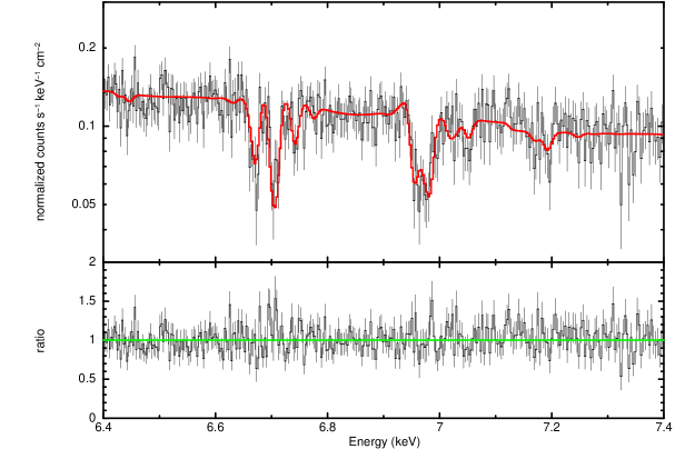
Figure 1.— The third-order spectrum of GRS 1915$+$105. The best-fit model based on joint fits to the first and third-order spectra is shown in red (see Table 1). Four photoionization zones with paired absorption and re-emission are required to fit the data. The He-like Fe XXV line is resolved into intercombination and resonance lines (rest frame energy: 6.700 keV). Instances of H-like Fe XXVI absorption lines close to the rest-frame value of 6.970 keV, and blue-shifted up to 7.05 keV and 7.2 keV are apparent. The Fe XXVI line shape is a doublet owing to the expected spin-orbit splitting in the H-like atom.

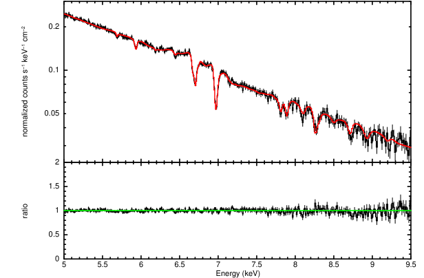
Figure 2.— The first-order spectrum of GRS 1915$+$105. The best-fit model is shown in red (see the text, and Table 1).

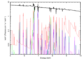
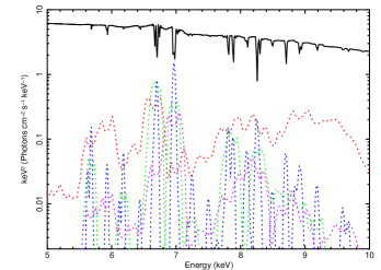
Figure 3.— Dynamical broadening plays an important role in shaping the re-emission spectrum of the wind. Zones 1–4 are depicted in red, green, blue, and magenta, respectively. Left: Dynamical broadening has been removed from the model in Table 1, yielding wind re-emission lines that are much sharper than the data. Right: The spectral model detailed in Table 1, with the blurring required by the data.

Figure 4.— First-order HEG spectra of GRS 1915$+$105 from the soft states observed in 2007 and 2015. The spectra are shown as a ratio to the best-fit continuum, with the best-fit wind spectrum plotted through the ratio. In this representation, the presence of accretion disk P Cygni line profiles is clear. Top: Data from the 2007 soft state, with the model of Miller et al. (2015). Middle: Data from the 2015 soft state, with the corresponding best-fit model (see Figure 2 and Table 1). Bottom: The 2007 and 2015 data and respective models are plotted together. The similarity of the spectra suggests that a particular wind geometry manifests in soft states.

Table 1Spectral Fitting Results and Derived Wind Parameters

Parameter	Zone 1	Zone 2	Zone 3	Zone 4	Continuum
${\rm N}_{\rm H}~{}(10^{22}~{}{\rm cm}^{-2})$	$30(2)$	$0.65(5)$	$1.0(3)$	$2.5^{+2.5}_{-1.2}$	–
log($\xi$)	$4.04(2)$	$3.87(5)$	$4.5(1)$	$4.7(5)$	–
$v/c~{}(10^{-3})$	$-0.70(5)$	$-6.2(3)$	$-11.0(5)$	$-30.5(5)$	–
$R~{}({\rm GM/c^{2}})$	$850^{+250}_{-50}$	$3000^{+600}_{-400}$	$30,000_{-2000}$	$1200^{+300}_{-300}$	–
$\theta$ (deg)	$60^{+7}$	$60^{+7}$	$60^{+7}$	$60^{+7}$	–
emis. norm.	$0.10^{+0.01}$	$0.21(2)$	$0.38(7)$	$0.5*$	–
$n~{}(10^{15}~{}{\rm cm}^{-3})$	20(5)	2.4(6)	0.006(1)	2.2(3)	–
$\dot{\rm M}_{wind}~{}(10^{18}~{}{\rm g}~{}{\rm s}^{-1})$	0.73(6)	10(1)	4.0(9)	8(8)	–
$\dot{\rm M}_{wind}~{}(10^{-8}~{}{\rm M}_{\odot}~{}{\rm yr}^{-1})$	1.2(1)	15(2)	6(2)	1(1)	–
$\dot{\rm M}_{wind}/\dot{\rm M}_{accr.}$	0.18(2)	2.3(3)	1.0(3)	2(2)	–
$L_{kin}(10^{34}~{}{\rm erg}~{}{\rm s}^{-1})$	0.016(2)	17(2)	22(5)	30(30)	–
$f~{}(10^{-2})$	1.3(4)	0.06(2)	4(1)	0.1(1)	–
${\rm log}({\rm T}_{wind})$	6.5(2)	6.0(2)	7.0(2)	7.0(2)	–
$|B_{MHD}|$ ($10^{4}$ Gauss)	2.1(8)	0.4(2)	0.06(2)	1.(1)	–
$|B_{MCF}|$ ($10^{4}$ Gauss)	80(30)	14(6)	5(2)	30(30)	–
$|B_{\alpha}|$ ($10^{4}$ Gauss)	30-100	20-60	1.4-2.6	70-230	–
kT (keV)	–	–	–	–	1.521(3)
disk norm.	–	–	–	–	$139(1)$
$\Gamma$	–	–	–	–	$2.8(1)$
power-law norm.	–	–	–	–	$11.0(7)$
$\sigma$ (keV)	–	–	–	–	0.08(1)
Gauss norm. $(10^{-3})$	–	–	–	–	2.2(2)

References

- (1)
- (2) Arnaud, K., 1996, Astronomical Data Analysis Software and Systems V, ASP Converence Series, eds. G. H. Jacoby and J. Barnes, 101, 17
- (3)
- (4) Begelman, M. C., McKee, C. F., & Shields, G. A., 1983, ApJ, 271, 70
- (5)
- (6) Begelman, M. C., Armitage, P. J., Reynolds, C. S., 2015, ApJ, 809, 118
- (7)
- (8) Calvet, N., Hartmann, L., & Kenyon, S. J., 1993, ApJ, 402, 623
- (9)
- (10) Chakravorty, S., Petrucci, P.-O., Ferreira, J., Henri, G., Belmont, R., Clavel, M., Corbel, S., Rodriguez, J., Coriat, M., Drappeau, S., Malzac, J, 2016, A&A, in press, arxiv:1512.09149
- (11)
- (12) Churazov, E., Gilfanov, M., Forman, W., Jones, C., 1996, ApJ, 471, 673
- (13)
- (14) Fabian, A. C., Rees, M. J., Stella, L., White, N. E., 1989, MNRAS, 238, 729
- (15)
- (16) Fukumura, K., Tombesi, F., Kazanas, D., Shrader, C., Behar, E., Contopoulos, I., 2014, ApJ, 780, 120
- (17)
- (18) Fukumura, K., Tombesi, F., Kazanas, D., Shrader, C., Behar, E., Contopoulos, I., 2015, ApJ, 805, 17
- (19)
- (20) Higginbottom, N., & Proga, D., 2015, ApJ, 807, 107
- (21)
- (22) Kallman, T. R., & Bautista, M. A., 2001, ApJS, 133, 221
- (23)
- (24) Kallman, T. R., Bautista, M. A., Goriely, S., Mendoza, C., Miller, J. M., Palmieri, P., Quinet, P., Raymond, J., 2009, ApJ, 701, 865
- (25)
- (26) King, A. L., Miller, J. M., Raymond, J., Fabian, A. C., Reynolds, C. S., Kallman, T. R., Maitra, D., Cackett, E. M., Rupen, M. P., 2012, ApJ, 746, L20
- (27)
- (28) King, A. L., Miller, J. M., Raymond, J., Fabian, A. C., Reynolds, C. S., Gultekin, K., Cackett, E. M., Allen, S. W., Proga, D., Kallman, T. R., 2013, ApJ, 762, 103
- (29)
- (30) Lee, J. C., Reynolds, C. S., Remillard, R., Schulz, N. S., Blackman, E. G., Fabian, A. C., 2002, ApJ, 567, 1102
- (31)
- (32) McClintock, J., Shafee, R., Narayan, R., Remillard, R., Davis, S., Li, L., 2006, ApJ, 652, 518
- (33)
- (34) Miller, J. M., Raymond, J., Fabian, A., Steeghs, D., Homan, J., Reynolds, C., van der Klis, M., Wijnands, R., 2006, Nature, 441, 953
- (35)
- (36) Miller, J. M., Raymond, J., Homan, J., Fabian, A. C., Steeghs, D., Wijnands, R., Rupen, M., Charles, P., van der Klis, M., Lewin, W. H. G., 2006b, ApJ, 646, 394
- (37)
- (38) Miller, J. M., Raymond, J., Reynolds, C. S., Fabian, A. C., Kallman, T. R., Homan, J., 2008, ApJ, 680, 1359
- (39)
- (40) Miller, J. M., et al., 2013, ApJ, 775, L45
- (41)
- (42) Miller, J. M., Fabian, A. C., Kaastra, J., Kallman, T., King, A. L., Proga, D., Raymond, J., Reynolds, C. S., 2015, ApJ, 814, 87
- (43)
- (44) Miller, K. A., & Stone, J. M., 2000, ApJ, 534, 398
- (45)
- (46) Mitsuda, K., Inoue, H., Koyama, K., Makishima, K., Matsuoka, M., Ogawara, Y., Suzuki, K., Tanaka, Y., Shibazaki, N., Hirano, T., 1984, PASJ, 37, 741
- (47)
- (48) Neilsen, J., & Lee, J. C., 2009, Nature, 458, 481
- (49)
- (50) Ponti, G., Fender, R. P., Begelman, M. C., Dunn, R., Neilsen, J., Coriat, M., 2012, MNRAS, 442, L11
- (51)
- (52) Proga, D., 2003, ApJ, 585, 406
- (53)
- (54) Proga, D., & Kallman, T., 2002, ApJ, 565, 455
- (55)
- (56) Remillard, R. A., & McClintock, J. E., 2006, ARA&A, 44, 49
- (57)
- (58) Reynolds, C. S., 2012, ApJ, 759, L15
- (59)
- (60) Reynolds, C. S., & Fabian, A. C., 2008, ApJ, 675, 1048
- (61)
- (62) Reynolds, M., & Miller, J. M., 2013, ApJ, 769, 16
- (63)
- (64) Salvesen, G., Simon, J., Armitage, P. J., Begelman, M., 2016, MNRAS, 457, 857
- (65)
- (66) Shafee, R., Narayan, R., McClintock, J., 2008, ApJ, 676, 549
- (67)
- (68) Sim, S., Proga, D., Miller, L., Long, K., Turner, T. J., 2010, MNRAS, 408, 1396
- (69)
- (70) Steeghs, D., McClintock, J. E., Parsons, S. G., Reid, M. J., Littlefair, S., Dhillon, V. S., 2013, ApJ, 768, 185
- (71)
- (72) Ueda, Y., Yamaoka, K., Remillard, R., 2009, ApJ, 695, 888
- (73)
- (74) Wilms, J., Allen, A., McCray, R., 2000, ApJ, 542, 914
- (75)
- (76) Woods, D. T., Klein, R. I., Castor, J. I., McKee, C. F., & Bell, J. B., 1996, ApJ, 461, 767
- (77)