Modeling and related results for current-actuated piezoelectric beams by including magnetic effects

Abstract

Piezo-electric material can be controlled with current as the electrical variable, instead of voltage. The main purpose of this paper is to derive the governing equations for a current-controlled piezo-electric beam and to investigate stabilizability. Besides the consideration of current control, there are several new aspects to the model here. Most significantly, magnetic effects are included. For the electromagnetic part of the model, electrical potential and magnetic vector potential are chosen to be quadratic-through thickness to include the induced effects of the electromagnetic field. Two sets of decoupled system of partial differential equations are obtained; one for stretching motion and another one for bending motion. Hamilton’s principle is used to derive a boundary value problem that models a single piezo-electric beam actuated by a charge (or current) source at the electrodes. Current or charge controllers at the electrodes can only control the stretching motion. Attention is therefore focused on control of the stretching equations in this paper. It is shown that the Lagrangian of the beam is invariant under certain transformations. A Coulomb-type gauge condition which is widely used in the electromagnetic theory is used here. This gauge condition decouples the electrical potential equation from the equations of the magnetic potential. A semigroup approach is used to prove that the Cauchy problem is well-posed. Unlike the voltage or charge actuation, a bounded control operator in the natural energy space is obtained in the current actuation case. The paper concludes with analysis of stabilizability and comparison with other actuation approaches and models.

1 Introduction

Piezoelectric materials are elastic beam/plates covered by electrodes at the top and bottom surfaces, insulated at the edges (to prevent fringing effects), and connected to an external electric circuit. (See Figure 1.) They convert mechanical energy to electrical and magnetic energy, and vice versa. These materials are widely used in civil, aeronautic and space structures due to their small size and high power density. These materials can be actuated by either external mechanical forces or electrical forces. There are mainly three ways to (electrically) actuate piezoelectric materials: voltage, current or charge. Piezoelectric materials have been traditionally activated by a voltage source [3, 4, 9, 27, 28, 30, 31, 32]. It is well-known that the control operator is unbounded in the energy space if the piezoelectric structure is controlled by a voltage or a charge source, for instance see [2, 9, 16, 21, 28].

Hysteresis occurs in the voltage-strain relationship for piezo-electric structures; see for instance, [28]. This complicates control of these materials. One way to avoid hysteresis is by applying only low voltages, but this prevents these structures from being used at their maximum potential. Therefore controller design needs to consider hysteresis in order to obtain maximum accuracy and effectiveness. Some approaches are passivity [14] and inverse compensation [29]. Another way to reduce the hysteresis is current or charge actuation, see for instance [6, 12, 15, 19, 20, 23]. Existing models for current control use only circuit equations attached to the standard elastic beam equations, and magnetic effects are not considered. Magnetic effects, even though small, were previously shown to be very important to the controllability and stabilizability of piezoelectric beams [33]. In fact, it has been shown [21] that voltage-controlled beams cannot even be asymptotically stabilized for certain material parameters.

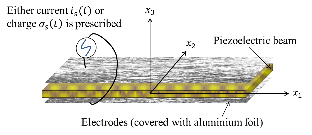
Fig. 1: When either charge $\sigma_{s}(t)$ or current $i_{s}(x,t)$ is prescribed to the electrodes, an electric field is created between the electrodes, and therefore the beam/plate either shrinks or extends. Unlike the voltage actuation, the input-output hysteresis reduces substantially.

In this paper, dynamic magnetic effects are included in the derivation of a model for piezoelectric beams actuated by a current (or charge) source. The electromagnetic field is described in terms of scalar electric potential and magnetic vector potential, After deriving expressions the various contributions to the energy, Hamilton’s Principle is used to derive a system of partial differential equations modelling the coupling between the mechanical and the electro-magnetic dynamics. These equations do not have a unique solution since the potentials are not uniquely determined. This is because the Lagrangian corresponding to Maxwell’s equations is invariant under certain transformations; for instance see [8, page 80]). Obtaining a system of equations with a unique solution requires a appropriate gauge condition. A number of gauges are possible. A Coulomb type of transformation is used here. Implementation of this transformation simplifies the equations considerably. The original highly coupled system of equations becomes a system of equations where the equations corresponding to the electrical variables are completely decoupled from the ones involving magnetic potential variables. Well-posedness of the model in an appropriate Hilbert space is then established. The norm in the Hilbert space corresponds to the energy of the system. It is shown that the spectrum of the generator consists entirely of imaginary eigenvalues. Stabilizability of the model is compared to voltage control, as well as to the case where magnetic effects are neglected. Some of the results presented in this paper, in particular, Lemma 2.1, Theorem 3.1, Theorems 4.1, 4.2 and a weaker version of Theorem 5.1 were previously reported in the conference paper [22].

$A$	Magnetic potential vector	$\rho$	Mass density per unit volume
$B$	Magnetic flux density vector	$n$	Surface unit outward normal vector
$c,\alpha$	Elastic stiffness coefficients	$\sigma_{s}$	Surface charge density
$D$	Electric displacement vector	$\sigma_{b}$	Volume charge density
$E$	Electric field intensity vector	$S$	Strain tensor
$\varepsilon$	Permittivity coefficients	$T$	Stress tensor
$h$	Thickness of the beam	$U_{1}$	$x_{1}$ component of the displacement field
$i_{b}$	Volume current density	$U_{3}$	$x_{3}$ component of the displacement field
$i_{s}$	Surface current density	$v$	Longitudinal disp. of the centerline of the beam
$\phi$	Electric potential	$V$	Voltage
$\gamma$	Piezoelectric coefficients	$w$	Transverse displacement of the beam
$\mu$	Magnetic permeability of beams

Table 1: Notation

2 Physical Model

Let $x_{1},x_{2}$ be the longitudinal directions, and $x_{3}$ be the transverse directions (see Figure 1). Assume that the piezoelectric beam occupy the region $\Omega=[0,L]\times[-r,r]\times[-\frac{h}{2},\frac{h}{2}]$ with the boundary $\partial\Omega,$ the electroded region and the insulated region, where $L>>h.$ Throughout this paper, dots denote differentiation with respect to time, that is $\dot{x}(t)=\frac{dx}{dt}.$

A very widely-used linear constitutive relationship [31] for piezoelectric beams is

$$\left(\begin{array}[]{l}T\\ D\\ \end{array}\right)=\left[{\begin{array}[]{*{20}c}c&-\gamma^{\text{T}}\\ \gamma&\varepsilon\\ \end{array}}\right]\left(\begin{array}[]{l}S\\ E\\ \end{array}\right)$$ (7)

where $T=(T_{11},T_{22},T_{33},T_{23},T_{13},T_{12})^{\rm T}$ is the stress vector,
$S=(S_{11},S_{22},S_{33},S_{23},S_{13},S_{12})^{\rm T}$ is the strain vector, $D=(D_{1},D_{2},D_{3})^{\text{T}}$ and $E=(E_{1},E_{2},E_{3})^{\text{T}}$ are the electric displacement and the electric field vectors, respectively, and moreover, the matrices $[c],[\gamma],[\varepsilon]$ are the matrices with elastic, electro-mechanic and dielectric constant entries (for more details see [31]). Under the assumption of transverse isotropy and polarization in $x_{3}-$direction, these matrices reduce to

$$c=\left({\begin{array}[]{*{20}c}{c_{11}}&{c_{12}}&{c_{13}}&0&0&0\\ {c_{21}}&{c_{22}}&{c_{23}}&0&0&0\\ {c_{31}}&{c_{32}}&{c_{33}}&0&0&0\\ 0&0&0&c_{44}&0&0\\ 0&0&0&0&c_{55}&0\\ 0&0&0&0&0&c_{66}\end{array}}\right),~{}~{}~{}~{}\Gamma=\left({\begin{array}[]{*{20}c}0&0&0&0&\gamma_{15}&0\\ 0&0&0&-\gamma_{15}&0&0\\ \gamma_{31}&\gamma_{31}&\gamma_{33}&0&0&0\end{array}}\right)$$ (17)

$$\varepsilon=\left({\begin{array}[]{*{20}c}\varepsilon_{11}&0&0\\ 0&\varepsilon_{22}&0\\ 0&0&\varepsilon_{33}\\ \end{array}}\right)$$ (21)

We assume that all forces acting in the $x_{2}$ direction are zero which implies a beam. Moreover, $T_{33}$ is also assumed to be zero. Therefore

$$T=(T_{11},T_{13})^{\text{T}},S=(S_{11},S_{13})^{\text{T}},D=(D_{1},D_{3})^{\text{T}},E=(E_{1},E_{3})^{\text{T}}$$

and (7) reduces to

$$\left(\begin{array}[]{l}T_{11}\\ T_{13}\\ D_{1}\\ D_{3}\end{array}\right) =\left({\begin{array}[]{*{20}c}{c_{11}}&0&0&-\gamma_{31}\\ 0&{c_{55}}&-\gamma_{15}&0\\ 0&\gamma_{15}&\varepsilon_{11}&0&\\ \gamma_{31}&0&0&\varepsilon_{55}\\ \end{array}}\right)\left(\begin{array}[]{l}S_{11}\\ S_{13}\\ E_{1}\\ E_{3}\end{array}\right).$$ (34)

Let $(U_{1},U_{3})$ denote the displacement field vector of a point $(x_{1},x_{3}).$ Continuing with the Euler-Bernoulli beam small-displacement assumptions, the displacement field is given as the following

$$U_{1}=v-x_{3}\frac{\partial w}{\partial x_{1}},\quad U_{3}=w$$ (35)

where $v=v(x_{1})$ and $w=w(x_{1})$ denote the longitudinal displacement of the center line in $x_{1}$ direction, and transverse displacement of the beam, respectively. Since $S_{13}=\frac{1}{2}\left(\frac{\partial U_{1}}{\partial x_{3}}+\frac{\partial U_{3}}{\partial x_{1}}\right)=0,$ the only nonzero strain component is given by

$$S_{11}=\frac{\partial U_{1}}{\partial x_{1}}=\frac{\partial v}{\partial x_{1}}-x_{3}\frac{\partial^{2}w}{\partial x_{1}^{2}}.$$ (36)

To keep the notation simple let

$$\alpha=c_{11},\quad\gamma=\gamma_{31},\quad\gamma_{1}=\gamma_{15},\quad\varepsilon_{1}=\varepsilon_{11},\quad\varepsilon_{3}=\varepsilon_{33}.$$ (37)

With the new notation, the linear constitutive equations for an Euler-Bernoulli piezoelectric beam are

$$\left\{\begin{array}[]{ll}T_{11}=\alpha S_{11}-\gamma E_{3}&\\ T_{13}=-\gamma_{1}E_{1}&\\ D_{1}=\varepsilon_{1}E_{1}&\\ D_{3}=\gamma S_{11}+\varepsilon_{3}E_{3}&\end{array}\right.$$ (42)

Let $\mathbf{K},\mathbf{P},\mathbf{E}$ and $\mathbf{B}$ be kinetic, potential, electrical, and magnetic energies of the beam, respectively, and let $\mathbf{W}$ be the work done by the external forces. To model charge or current-actuated piezoelectric beams we use the following Lagrangian [18]

$$\mathbf{L}=\int_{0}^{T}\left[\mathbf{K}-(\mathbf{P}-\mathbf{E}+\mathbf{B})+\mathbf{W}\right]dt$$ (43)

for which we use the constitutive equations (42) where the pair $(S,E)$ belongs to the set of independent variables. In the above, $\mathbf{P}-\mathbf{E}+\mathbf{B}$ is called electrical enthalpy. Note that in modeling piezoelectric beams by voltage-actuated electrodes we use a different Lagrangian

$$\tilde{\mathbf{L}}=\int_{0}^{T}\left[\mathbf{K}-(\mathbf{P}+\mathbf{E})+\mathbf{B}+\mathbf{W}\right]~{}dt$$ (44)

for which the constitutive equations (42) are written in terms of the independent variables $(S,D).$ The Lagrangian $\tilde{\mathbf{L}}$ can be obtained by applying a Legendre transformation to $\mathbf{L}.$ Here $\mathbf{P}+\mathbf{E}$ denotes the total stored energy of the beam, and $\mathbf{B}$ acts as the electrical kinetic energy of the beam. This case is studied in [21]. Depending on the prescribed quantity at the electrodes, Lagrangian is chosen either $\mathbf{L}$ or $\tilde{\mathbf{L}}.$

The full set of Maxwell’s equations is; see for example [10, Page 332]),

$$\nabla\cdot D=~{}\sigma_{b}\quad{\rm{in}}\quad\Omega\times\mathbb{R}^{+}~{}\quad$$ (Electric Gauss’s  law) (45)

$$\nabla\cdot B=~{}0\quad{\rm{in}}\quad\Omega\times\mathbb{R}^{+}~{}\quad$$ (Gauss’s law of magnetism)

$$\nabla\times E=~{}-\dot{B}\quad{\rm{in}}\quad\Omega\times\mathbb{R}^{+}~{}\quad$$ (Faraday’s law)

$$\frac{1}{\mu}(\nabla\times B)=~{}i_{b}+\dot{D}\quad{\rm{in}}\quad\Omega\times\mathbb{R}^{+}~{}\quad$$ (Ampére-Maxwell law)

with one of the essential electric boundary conditions prescribed on the electrodes

$$-D\cdot n=~{}\sigma_{s}(t) \quad{\rm{on}}\quad{\partial\Omega}\times\mathbb{R}^{+}~{}\quad$$ (Charge ) (46)

$$\frac{1}{\mu}(B\times n)=~{}i_{s}(t) \quad{\rm{on}}\quad{\partial\Omega}\times\mathbb{R}^{+}~{}\quad$$ (Current) (47)

$$\phi=~{}V(t) \quad{\rm{on}}\quad{\partial\Omega}\times\mathbb{R}^{+}~{}\quad$$ (Voltage) (48)

and appropriate mechanical boundary conditions at the edges of the beam (the beam is clamped, hinged, free, etc.). Here $B$ denotes the magnetic field vector, and $\sigma_{b},i_{b},\sigma_{s},\\ i_{s},V,\mu,n$ denote body charge density, body current density, surface charge density, surface current density, voltage, magnetic permeability, and unit normal vector to the surface $\partial\Omega,$ respectively. In this paper we consider only current and charge-driven electrodes (i.e. we ignore(48)). The voltage-driven electrode case is handled in details in [21]. In modeling piezoelectric beams, there are mainly three approaches including electric and magnetic effects [31]:

i) Electrostatic electric field:

Electrostatic electric field approach is the most widely-used approach in the literature. It completely ignores magnetic effects: $B=\dot{D}=i_{b}=\sigma_{b}=0.$ Maxwell’s equations (45) reduce to $\nabla\cdot D=0$ and $\nabla\times E=0.$ Therefore, there exist a scalar electric potential such that $E=-\nabla\phi$ and $\phi$ is determined up to a constant.

ii) Quasi-static electric field:

This approach rules out some of the magnetic effects (non-magnetizable materials) [31]: $\sigma_{b}=i_{b}=0.$ However, $\dot{D}$ and $B$ are non-zero. Therefore, (45) reduce to

$$\nabla\cdot D=0,~{}~{}~{}\nabla\cdot B=0,~{}~{}~{}\dot{B}=-\nabla\times E,~{}~{}~{}\dot{D}=\frac{1}{\mu}(\nabla\times B).$$

The equation $\nabla\cdot B=0$ implies that there exists a vector $A$ such that $B=\nabla\times A.$ This vector is called the magnetic potential . It follows from substituting $B$ to $\dot{B}=-\nabla\times E$ that there exists a scalar electric potential $\phi$ such that

$$E=-\dot{A}-\nabla\phi.$$ (49)

where $\dot{A}$ stands for the induced electric field due to the time-varying magnetic effects. One simplification in this approach is to ignore $A$ and $\dot{A}$ since $A,\dot{A}\ll\phi.$ With this assumption $\dot{D}$ may be non-zero.

iii) Fully dynamic electric field:

Unlike the quasi-static assumption, $A$ and $\dot{A}$ are left in the model. Depending on the type of material, body charge density $\sigma_{b}$ and body current density $i_{b}$ can also be non-zero. Note that even though the displacement current $\dot{D}$ is assumed to be non-zero in both quasi-static and fully dynamic approaches, the term $\ddot{D}$ is zero in quasi-static approach since $\dot{A}=0.$

Since the piezoelectric materials are not perfectly insulated, the electric field $E$ causes currents to flow when conductivity occurs. Therefore the time-dependent equation of the continuity of electric charge must be employed. In this paper, we follow the fully dynamic approach to include all of the magnetic effects. If we take the divergence of both sides of Ampére-Maxwell equation (45), we obtain

$$\frac{1}{\mu}\nabla\cdot\left(\nabla\times B\right)=\nabla\cdot i_{b}+\nabla\cdot\dot{D}.$$ (50)

The term on the left hand side of the equation above is zero, and therefore by using Gauss’s law (45), we obtain the following electric continuity condition

$$\dot{\sigma}_{b}+\nabla\cdot i_{b}=0\quad{\text{i}n}~{}~{}\Omega$$ (51)

The physical interpretation of (51) is the local conservation of electrical charge. From (45)

$$\frac{1}{\mu}\int_{\partial\Omega}\left(\nabla\times B\right)\cdot n~{}dS=\int_{\partial\Omega}\left(i_{b}\cdot n+\dot{D}\cdot n\right)~{}dS,$$

and use the charge boundary conditions (46) with $i_{s}(x,t)\equiv 0$

$$0=\frac{1}{\mu}\int_{\partial\Omega}\nabla\times B\cdot n~{}dS = \int_{\partial\Omega}\left(i_{b}^{3}-\dot{\sigma}_{s}\right)~{}dS$$

or, alternatively, use the current boundary condition (47) with $\sigma_{s}\equiv 0$

$$\frac{1}{\mu}\int_{\partial\Omega}\nabla\times B\cdot n~{}dS = \int_{\partial\Omega}i_{b}^{3}~{}dS$$

where $n$ is the outward unit normal vector on $\partial\Omega.$ Hence we obtain surface electric continuity conditions (or compatibility conditions)

$$\dot{\sigma}_{s}-i_{b}^{3}=0,\quad{\rm or,}\quad\frac{di_{s}}{dx}-i_{b}^{3}=0\quad\text{on}~{}\partial\Omega.$$ (52)

For more details, the reader can refer to [11, Section 3.9].

Henceforth, to simplify the notation, $x=x_{1}$ and $z=x_{3}.$

Note that piezoelectricity is the direct result of piezoelectric effect, which is, once the external electric field is applied to the electrodes, strain is produced and therefore the beam/plate extends or shrinks (direct effect), whereas, when the plate/beam extends and shrink, it produces electric voltage which is so-called the induced (inverse) effect. The linear through-thickness assumption of the electric potential $\phi(x,z)=\phi^{0}(x)+z\phi^{1}(x)$ completely ignores the induced potential effect since $\phi$ is completely known as a function of voltage. For example, when the voltage is prescribed at the electrodes, i.e. $\phi\left(\frac{h}{2}\right)=V$ and $\phi\left(-\frac{h}{2}\right)=0,$ we have

$$\phi=\frac{V}{2}+z\frac{V}{h},$$

and therefore the electric field component in the transverse direction $E_{3}$ becomes uniform in the transverse direction, i.e. $E_{3}=-\phi^{1}=-\frac{V}{h},$ as we consider electrostatic and quasi-static assumptions. Therefore the induced effect is ignored in the linear-through thickness assumption. In this paper, we use a quadratic-through thickness potential distribution that takes care of the induced effect and improves the modeling accuracy:

$$\phi(x,z)=\phi^{0}(x)+z\phi^{1}(x)+\frac{z^{2}}{2}\phi^{2}(x).$$ (53)

Since we are in the beam theory, we assume that the magnetic vector potential $A$ has nonzero components only in $x$ and $z$ directions. To keep the consistency with $\phi$, we assume that $A$ is quadratic through-thickness as well:

$$A(x,z)=\left(\begin{array}[]{c}A_{1}(x,z)\\ 0\\ A_{3}(x,z)\\ \end{array}\right)=\left(\begin{array}[]{c}A_{1}^{0}(x)+zA_{1}^{1}(x)+\frac{z^{2}}{2}A_{1}^{2}(x)\\ 0\\ A_{3}^{0}(x)+zA_{3}^{1}(x)+\frac{z^{2}}{2}A_{3}^{2}(x)\\ \end{array}\right).$$ (60)

By (49)

$$E_{1}=-\left(\dot{A}_{1}^{0}+z\dot{A}_{1}^{1}+\frac{z^{2}}{2}\dot{A}_{1}^{2}\right)-\left(({\phi}^{0})_{x}+z(\phi^{1})_{x}+\frac{z^{2}}{2}(\phi^{2})_{x}\right),$$

$$E_{3}=-\left(\dot{A}_{3}^{0}+z\dot{A}_{3}^{1}+\frac{z^{2}}{2}\dot{A}_{3}^{2}\right)-\left(\phi^{1}+z\phi^{2}\right).$$ (61)

Now we use the constitutive equations (42) along with (35), (36), and (53)-(61) to write

$$\mathbf{E}-\mathbf{P} = \frac{1}{2}\int_{\Omega}\left(D_{1}E_{1}+D_{3}E_{3}-T_{11}S_{11}-T_{13}S_{13}\right)~{}dX$$ (62)

$$= \frac{1}{2}\int_{\Omega}\left(-\alpha S_{11}^{2}+2\gamma S_{11}E_{3}+{\varepsilon_{1}}E_{1}^{2}+{\varepsilon_{3}}E_{3}^{2}\right)~{}dX$$

$$= \frac{1}{2}\int_{0}^{L}\left[-{\alpha}h\left(v_{x}^{2}+\frac{h^{2}}{12}w_{xx}^{2}\right)-2{\gamma}h\left(\left(\phi^{1}+\dot{A}_{3}^{0}+\frac{h^{2}}{24}\dot{A}_{3}^{2}\right)v_{x}-\frac{h^{2}}{12}w_{xx}\left(\phi^{2}+\dot{A}_{3}^{1}\right)\right)\right.$$

$$\quad+{{\varepsilon_{1}}}h\left((\phi^{0}_{x})^{2}+\frac{h^{2}}{12}(\phi^{1}_{x})^{2}+\frac{h^{4}}{320}(\phi^{2}_{x})^{2}+(\dot{A}_{1}^{0})^{2}+\frac{h^{2}}{12}(\dot{A}_{1}^{1})^{2}+\frac{h^{4}}{320}(\dot{A}_{1}^{3})^{2}\right)$$

$$\quad+{{\varepsilon_{3}}}h\left((\phi^{1})^{2}+\frac{h^{2}}{12}(\phi^{2})^{2}+(\dot{A}_{3}^{0})^{2}+\frac{h^{2}}{12}(\dot{A}_{3}^{1})^{2}+\frac{h^{4}}{320}(\dot{A}_{3}^{2})^{2}\right)$$

$$\quad+2{{\varepsilon_{1}}}h\left((\phi^{0})_{x}\dot{A}_{1}^{0}+\frac{h^{2}}{24}(\phi^{0})_{x}(\phi^{2})_{x}+\frac{h^{2}}{24}\dot{A}_{1}^{0}\dot{A}_{1}^{2}+\frac{h^{2}}{24}(\phi^{0})_{x}\dot{A}_{1}^{2}\right.$$

$$\left.\quad\quad\quad\quad\quad+\frac{h^{2}}{24}(\phi^{2})_{x}\dot{A}_{1}^{0}+\frac{h^{2}}{12}(\phi^{1})_{x}\dot{A}_{1}^{1}+\frac{h^{4}}{320}(\phi^{2})_{x}\dot{A}_{1}^{2}\right)$$

$$\quad\left.\quad+2{{\varepsilon_{3}}}h\left(\phi^{1}\dot{A}_{3}^{0}+\frac{h^{2}}{24}\dot{A}_{3}^{0}\dot{A}_{3}^{2}+\frac{h^{2}}{24}\phi^{1}\dot{A}_{3}^{2}+\frac{h^{2}}{12}\phi^{2}\dot{A}_{3}^{0}\right)\right]~{}dx,$$

$$\mathbf{B} = \frac{\mu}{2}\int_{\Omega}(\nabla\times A)\cdot(\nabla\times A)~{}dX$$ (63)

$$= \frac{\mu}{2}\int_{0}^{L}\int_{-h/2}^{h/2}\left(A_{1}^{1}+zA_{1}^{2}-(A_{3}^{0})_{x}-z(A_{3}^{1})_{x}-\frac{z^{2}}{2}(A_{3}^{2})_{x}\right)^{2}~{}dzdx$$

$$= \frac{\mu h}{2}\int_{0}^{L}\left[(A_{1}^{1})^{2}+\frac{h^{2}}{12}(A_{1}^{2})^{2}+((A_{3}^{0})_{x})^{2}+\frac{h^{2}}{12}((A_{3}^{1})_{x})^{2}+\frac{h^{4}}{320}((A_{3}^{2})_{x})^{2}\right.$$

$$\left.-2\left(A_{1}^{1}~{}(A_{3}^{0})_{x}+\frac{h^{2}}{24}A_{1}^{1}(A_{3}^{2})_{x}-\frac{h^{2}}{12}A_{1}^{2}(A_{3}^{1})_{x}-\frac{h^{2}}{24}(A_{3}^{0})_{x}(A_{3}^{2})_{x}\right)\right]~{}dx,\quad\quad\quad$$

$$\mathbf{K} = \frac{\rho}{2}\int_{\Omega}\left(\dot{U}_{1}^{2}+\dot{U}_{3}^{2}\right)~{}dX=\frac{\rho h}{2}\int_{0}^{L}\left(\dot{v}^{2}+\dot{w}^{2}+\frac{h^{2}}{12}\dot{w}_{x}^{2}\right)~{}dx,$$ (64)

Now we define the work $\mathbf{W}$ done by the external forces. We first define the body force resultants $i_{b},\sigma_{b},i_{s},\sigma_{s}$ as in [17]:

$$i_{b}=\int_{-h/2}^{h/2}\tilde{i}_{b}~{}dz,\quad\sigma_{b}=\int_{-h/2}^{h/2}\tilde{\sigma}_{b}~{}dz$$

$$i_{s}=\int_{-h/2}^{h/2}\tilde{i}_{s}~{}dz,\quad\sigma_{s}=\int_{-h/2}^{h/2}\tilde{\sigma}_{s}~{}dz.$$

In the above the surface charge density $\tilde{\sigma}_{s}$ and surface current density $\tilde{i}_{s}$ are independent of $z$ since they are given at the electrodes. For the Euler-Bernoulli beam, it is appropriate to assume that body charge $\tilde{\sigma}_{b}$ and body current $\tilde{i}_{b}$ are independent of $z,$

$$i_{b}=\tilde{i}_{b}h,\quad\sigma_{b}=\tilde{\sigma}_{b}h,\quad i_{s}=\tilde{i}_{s}h,\quad\sigma_{s}=\tilde{\sigma}_{s}h.$$

We choose either surface charge $\sigma_{s}$ or $i_{s}$ to be non-zero, and either $i_{b}$ or $\sigma_{b}$ to be nonzero, depending on the type of actuation. We assume that there are no mechanical external forces acting on the beam. The work done by the electrical external forces is [18]

$$\mathbf{W} = \int_{\Omega}\left(~{}-\tilde{\sigma}_{b}~{}\phi+\tilde{i}_{b}\cdot A\right)~{}dX+\int_{\partial\Omega}\left(-\tilde{\sigma}_{s}~{}\phi+\tilde{i}_{s}\cdot A\right)~{}dX$$ (65)

$$= \int_{\Omega}\left(~{}-\tilde{\sigma}_{b}~{}\phi+\tilde{i}_{b}^{1}A_{1}\right)~{}dX+\int_{\partial\Omega}\left(-\tilde{\sigma}_{s}~{}\phi+\tilde{i}_{s}^{1}\cdot A_{1}\right)~{}dX$$

$$= -\int_{0}^{L}\int_{-h/2}^{h/2}\tilde{\sigma}_{b}\left(\phi^{0}(x)+z\phi^{1}(x)+\frac{z^{2}}{2}\phi^{2}(x)\right)~{}dzdx$$

$$+\int_{0}^{L}\int_{-h/2}^{h/2}\tilde{i}_{b}^{1}\left(A_{1}^{0}(x)+zA_{1}^{1}(x)+\frac{z^{2}}{2}A_{1}^{2}\right)~{}dzdx$$

$$+\int_{0}^{L}\left(-\tilde{\sigma}_{s}\left(\phi(h/2)-\phi(-h/2)\right)+\tilde{i}_{s}^{1}\left(A_{1}(h/2)-A_{1}(-h/2)\right)\right)~{}dx$$

$$= \int_{0}^{L}\left(-\sigma_{b}\left(\phi^{0}+\frac{h^{2}}{24}\phi^{2}\right)-\sigma_{s}+i_{b}^{1}\left(A_{1}^{0}+\frac{h^{2}}{24}A_{1}^{2}\right)-\sigma_{s}~{}\phi^{1}+i_{s}^{1}~{}A_{1}^{1}\right)~{}dx$$

where $i_{s}(x,t)=(i_{s}^{1}(x,t),0,0),$ and $i_{b}(x,t)=(i_{b}^{1}(x,t),0,0).$ In the above $i_{s}$ has only one nonzero component since $i_{s}\perp B$, and $i_{s}\perp n$ by (47). Moreover, $i_{b}$ has only one nonzero component since we assumed that there is no force acting in the $x_{2}$ and $x_{3}$ directions.

If the magnetic effects are neglected, a variational approach cannot be used in the case of current actuation since $A\equiv 0$ and so $\mathbf{W}\equiv 0.$ This is very different from the charge and voltage actuation cases since for charge and voltage actuation $\mathbf{W}$ is not a function of $A.$

3 Derivation of Governing Equations

Assume that both ends of the piezoelectric beam are free. The application of Hamilton’s principle, setting the variation of Lagrangian $\mathbf{L}$ in (43) with respect to the all kinematically admissible displacements

$$\{v,w,\phi^{0},\phi^{1},\phi^{2},A_{1}^{0},A_{1}^{1},A_{1}^{2},A_{3}^{0},A_{3}^{1},A_{3}^{2}\}$$

to zero, yields stretching equations and bending equations respectively:

$$\left\{\begin{array}[]{l l}\rho h\ddot{v}-{\alpha}hv_{xx}-{\gamma}h\left((\phi^{1})_{x}+(\dot{A}_{3}^{0})_{x}+\frac{h^{2}}{24}(\dot{A}_{3}^{2})_{x}\right)=0&\\ -\frac{{{\varepsilon_{1}}}h^{3}}{12}\left((\phi^{1})_{xx}+(\dot{A}_{1}^{1})_{x}\right)+{{\varepsilon_{3}}}h\left(\dot{A}_{3}^{0}+\frac{h^{2}}{24}\dot{A}_{3}^{2}+\phi^{1}\right)-{\gamma}hv_{x}=\sigma_{s}&\\ \frac{{{\varepsilon_{1}}}h^{3}}{12}\ddot{A}_{1}^{1}+\frac{{{\varepsilon_{1}}}h^{3}}{12}(\dot{\phi}^{1})_{x}-\mu h\left((A_{3}^{0})_{x}+\frac{h^{2}}{24}(A_{3}^{2})_{x}-A_{1}^{1}\right)=i_{s}^{1}&\\ {{\varepsilon_{3}}}h\left(\ddot{A}_{3}^{0}+\frac{h^{2}}{24}\ddot{A}_{3}^{2}+\dot{\phi}^{1}\right)-\mu h\left((A_{3}^{0})_{xx}+\frac{h^{2}}{24}(A_{3}^{2})_{xx}-(A_{1}^{1})_{x}\right)-{\gamma}h\dot{v}_{x}=0&\\ \frac{{{\varepsilon_{3}}}h^{3}}{24}\left(\ddot{A}_{3}^{0}+\dot{\phi}^{1}\right)+\frac{{\varepsilon_{3}}h^{5}}{320}\ddot{A}_{3}^{2}-\mu h^{3}\left(\frac{h^{2}}{24}(A_{3}^{0})_{xx}+\frac{h^{2}}{320}(A_{3}^{2})_{xx}-\frac{1}{24}(A_{1}^{1})_{x}\right)&\\ \quad\quad\quad\quad\quad-\frac{{\gamma}h^{3}}{24}\dot{v}_{x}=0&\end{array}\right.$$ (66)

$$\left\{\begin{array}[]{l l}\rho h\ddot{w}-\frac{\rho h^{3}}{12}\ddot{w}_{xx}+\frac{{\alpha}h^{3}}{12}w_{xxxx}-\frac{{\gamma}h^{3}}{12}\left((\phi^{2})_{xx})+(\dot{A}_{3}^{1})_{xx}\right)=0&\\ -{{\varepsilon_{1}}}h\left((\phi^{0})_{xx}+\frac{h^{2}}{24}(\phi^{2})_{xx}+(\dot{A}_{1}^{0})_{x}+\frac{h^{2}}{24}(\dot{A}_{1}^{2})_{x}\right)=\sigma_{b}&\\ -\frac{{{\varepsilon_{1}}}h^{3}}{24}\left((\phi^{0})_{xx}+\frac{h^{2}}{24}(\phi^{2})_{xx}+(\dot{A}_{1}^{0})_{x}+\frac{h^{2}}{24}(\dot{A}_{1}^{2})_{x}\right)+\frac{{\gamma}h^{3}}{24}w_{xx}&\\ \quad\quad\quad\quad\quad-\frac{{{\varepsilon_{1}}}h^{5}}{720}(\phi^{2})_{xx}-\frac{{{\varepsilon_{1}}}h^{5}}{720}(\dot{A}_{1}^{2})_{x}+\frac{{{\varepsilon_{3}}}h^{3}}{12}\left(\phi^{2}+\dot{A}_{3}^{1}\right)=\frac{h^{2}\sigma_{b}}{24}&\\ {{\varepsilon_{1}}}h\left(\ddot{A}_{1}^{0}+\frac{h^{2}}{24}\ddot{A}_{1}^{2}+(\dot{\phi}^{0})_{x}+\frac{h^{2}}{24}(\dot{\phi}^{2})_{x}\right)=i_{b}^{1}&\\ \frac{{{\varepsilon_{1}}}h^{3}}{24}\left(\ddot{A}_{1}^{0}+\frac{h^{2}}{24}(\ddot{A}_{1}^{2})+(\dot{\phi}^{0})_{x}+\frac{h^{2}}{24}(\dot{\phi}^{2})_{x}\right)&\\ \quad\quad\quad\quad\quad+\frac{{{\varepsilon_{1}}}h^{5}}{720}\ddot{A}_{1}^{2}+\frac{{{\varepsilon_{1}}}h^{5}}{720}(\dot{\phi}^{2})_{x}+\frac{h^{3}\mu}{12}\left(A_{1}^{2}-(A_{3}^{1})_{x}\right)=\frac{h^{2}i_{b}^{1}}{24}&\\ \frac{{{\varepsilon_{3}}}h^{3}}{12}\left(\ddot{A}_{3}^{1}-\frac{\mu}{{{\varepsilon_{3}}}}(A_{3}^{1})_{xx}\right)+\frac{{{\varepsilon_{3}}}h^{3}}{12}\dot{\phi}^{2}+\frac{h^{3}\mu}{12}(A_{1}^{2})_{x}+\frac{{\gamma}h^{3}}{12}\dot{w}_{xx}=0&\end{array}\right.$$ (67)

with the natural boundary conditions at $x=0,L$

$$\left\{\begin{array}[]{r r}{\alpha}hv_{x}+{\gamma}h\left(\phi^{1}+\dot{A}_{3}^{0}+\frac{h^{2}}{24}\dot{A}_{3}^{2}\right)=0&{\rm{(Lateral~{}force)}}\\ \frac{h^{3}}{12}\left(-{\alpha}w_{xx}+{\gamma}\phi^{2}\right)=0&{\rm{(Bending~{}moment)}}\\ -\rho\ddot{w}_{x}+{\alpha}w_{xxx}-{\gamma}(\phi^{2})_{x}=0&{\rm{(Shear)}}\\ {\varepsilon_{1}}h\left(\dot{A}_{1}^{0}+\frac{h^{2}}{24}\dot{A}_{1}^{2}+({\phi}^{0})_{x}+\frac{h^{2}}{24}(\phi^{2})_{x}\right)=0&{\rm{(Charge)}}\\ \frac{{\varepsilon_{1}}h^{3}}{12}\left(\dot{A}_{1}^{1}+(\phi^{1})_{x}\right)=0&{\rm{(First~{}charge~{}moment)}}\\ {{\varepsilon_{1}}}h^{3}\left(\frac{1}{12}\dot{A}_{1}^{0}+\frac{h^{2}}{160}\dot{A}_{1}^{2}+\frac{1}{12}({\phi}^{0})_{x}+\frac{h^{2}}{160}(\phi^{2})_{x}\right)=0&{\rm{(Second~{}charge~{}moment)}}\\ \mu h\left(A_{1}^{1}-(A_{3}^{0})_{x}-\frac{h^{2}}{24}(A_{3}^{2})_{x}\right)=0&{\rm{(Current)}}\\ \frac{\mu h^{3}}{12}\left(A_{1}^{2}-(A_{3}^{1})_{x}\right)=0&{\rm{(First~{}current~{}moment)}}\\ \mu h^{3}\left(\frac{1}{24}A_{1}^{1}-\frac{1}{24}(A_{3}^{0})_{x}-\frac{h^{2}}{320}(A_{3}^{2})_{x}\right)=0&{\rm{(Second~{}current~{}moment)}}\end{array}\right.$$ (68)

The bending motion is described by the Rayleigh beam equation coupled to the electromagnetic equations. If the rotational inertia of the cross section of the beam is ignored, the terms $\ddot{w}_{xx}$ in (67)and $\ddot{w}_{x}$ in (68) go away.

The last equation in (66) can be simplified by using the previous one to get

$$\left\{\begin{array}[]{l l}\rho h\ddot{v}-{\alpha}hv_{xx}-{\gamma}h\left((\phi^{1})_{x}+(\dot{A}_{3}^{0})_{x}+\frac{h^{2}}{24}(\dot{A}_{3}^{2})_{x}\right)=0&\\ -\frac{{{\varepsilon_{1}}}h^{3}}{12}\left((\phi^{1})_{xx}+(\dot{A}_{1}^{1})_{x}\right)+{{\varepsilon_{3}}}h\left(\dot{A}_{3}^{0}+\frac{h^{2}}{24}\dot{A}_{3}^{2}+\phi^{1}\right)-{\gamma}hv_{x}=\sigma_{s}&\\ \frac{{{\varepsilon_{1}}}h^{3}}{12}\ddot{A}_{1}^{1}+\frac{{{\varepsilon_{1}}}h^{3}}{12}(\dot{\phi}^{1})_{x}-\mu h\left((A_{3}^{0})_{x}+\frac{h^{2}}{24}(A_{3}^{2})_{x}-A_{1}^{1}\right)=i_{s}^{1}&\\ {{\varepsilon_{3}}}h\left(\ddot{A}_{3}^{0}+\frac{h^{2}}{24}\ddot{A}_{3}^{2}+\dot{\phi}^{1}\right)-\mu h\left((A_{3}^{0})_{xx}+\frac{h^{2}}{24}(A_{3}^{2})_{xx}-(A_{1}^{1})_{x}\right)-{\gamma}h\dot{v}_{x}=0&\\ \frac{{{\varepsilon_{3}}}h^{3}}{24}\left(\ddot{A}_{3}^{0}+\frac{h^{2}}{24}\ddot{A}_{3}^{2}+\dot{\phi}^{1}\right)-\frac{\mu h^{3}}{24}\left((A_{3}^{0})_{xx}+\frac{h^{2}}{24}(A_{3}^{2})_{xx}-(A_{1}^{1})_{x}\right)&\\ \quad\quad\quad\quad\quad-\frac{{\gamma}h^{3}}{24}\dot{v}_{x}+\left(\frac{{{\varepsilon_{3}}}h^{5}}{720}\ddot{A}_{3}^{2}-\frac{\mu h^{5}}{720}(A_{3}^{2})_{xx}\right)=0\end{array}\right.$$ (69)

Note that the stretching (69) and bending (67) equations are completely decoupled when only one type of external electrical force is present. It will be assumed, as is common in practice, that there is no free body charge or current, i.e. $\sigma_{b}\equiv i_{b}\equiv 0.$ Then the bending equations (67) are entirely uncontrolled and also decoupled from the stretching equations (69). Therefore, from this point on, only the stretching equations (69) are considered with the corresponding boundary conditions at $x=0,L$

$$\left\{\begin{array}[]{l r}{\alpha}hv_{x}+{\gamma}h\left(\phi^{1}+\dot{A}_{3}^{0}+\frac{h^{2}}{24}\dot{A}_{3}^{2}\right)=0&{\rm{(Lateral~{}force)}}\\ \frac{{\varepsilon_{1}}h^{3}}{12}\left(\dot{A}_{1}^{1}+(\phi^{1})_{x}\right)=0&{\rm{(First~{}charge~{}moment)}}\\ \mu h\left(A_{1}^{1}-(A_{3}^{0})_{x}-\frac{h^{2}}{24}(A_{3}^{2})_{x}\right)=0&{\rm{(Current)}}\\ \frac{\mu h^{3}}{24}\left(A_{1}^{1}-(A_{3}^{0})_{x}-\frac{h^{2}}{24}(A_{3}^{2})_{x}\right)-\frac{\mu h^{5}}{720}(A_{3}^{2})_{x}=0&{\rm{(Second~{}current~{}moment)}}\end{array}\right.$$ (70)

The last two boundary conditions can also be simplified as

$$\left\{A_{1}^{1}-(A_{3}^{0})_{x}\right\}_{x=0,L}=\left\{(A_{3}^{2})_{x}\right\}_{x=0,L}=0.$$ (71)

The magnetic potential vector $A$ and the electric potential $\phi$ are not uniquely defined by (45). In fact, the Lagrangian $\mathbf{L}$ (43) is invariant under a large class of transformations.

Theorem 3.1.

For any scalar $C^{1}$ function $\chi=\chi(x,z,t),$ the Lagrangian $\mathbf{L}$ is invariant under the transformation

$$A\mapsto\tilde{A}:=A+\nabla\chi$$

$$\phi\mapsto\tilde{\phi}:=\phi-\dot{\chi}.$$ (72)

Proof: By (72), $\tilde{A}$ and $\tilde{\phi}$ satisfy

$$\tilde{B}=\nabla\times\tilde{A}=\nabla\times A+\nabla\times\nabla\chi=\nabla\times A=B$$

$$\tilde{E}=-\dot{\tilde{A}}-\nabla\tilde{\phi}=-\dot{A}-\nabla\dot{\chi}-\nabla\phi+\nabla\dot{\chi}=-\dot{A}-\nabla\phi=E.$$

This implies that $\mathbf{E}-\mathbf{P}$ and $\mathbf{B}$ defined respectively by (62) and (63) are invariant under the transformation. Since $\mathbf{K}$ in (64) is independent of $A$ and $\phi,$ we need to check if $\mathbf{W}$ defined by (65) is invariant under (72). We choose the arbitrary scalar function $\chi$ to be quadratic-through thickness $\chi=\chi^{0}+z\chi^{1}+\frac{z^{2}}{2}\chi^{2}$ to be consistent with the choices of $\varphi$ and $A$ in (53) and (60), respectively. We also assume that $\chi$ satisfies the stationary conditions $\left|\chi^{0}=\chi^{1}=\chi^{2}\right|_{t=0,T}=0$ for compatibility. By (72) we have

$$\tilde{A}_{1}^{0}=A_{1}^{0}+(\chi^{0})_{x},\quad A_{1}^{1}=A_{1}^{1}+(\chi^{1})_{x},\quad A_{1}^{2}=A_{1}^{2}+(\chi^{2})_{x},\quad\tilde{A}_{3}^{0}=A_{3}^{0}+\chi^{1},\quad\tilde{A}_{3}^{2}=A_{3}^{2},$$

$$\tilde{\phi}^{0}=\phi^{0}-\dot{\chi}^{0},\quad\tilde{\phi}^{1}=\phi^{1}-\dot{\chi}^{1},\quad\tilde{\phi}^{2}=\phi^{2}-\dot{\chi}^{2},$$

and therefore

$$\int_{0}^{T}{\tilde{\mathcal{W}}}~{}dt = \int_{0}^{T}\int_{0}^{L}\left(-\sigma_{b}\left({\tilde{\phi^{0}}}+\frac{h^{2}}{24}\tilde{\phi}^{2}\right)-\sigma_{s}~{}\tilde{\phi^{1}}+i_{b}^{1}\left(\tilde{A}_{1}^{0}+\frac{h^{2}}{24}\tilde{A}_{1}^{2}\right)+i_{s}^{1}~{}\tilde{A}_{1}^{1}\right)~{}dxdt$$

$$= \int_{0}^{T}\mathcal{W}dt+\int_{0}^{T}\int_{0}^{L}\left(\sigma_{b}\left(\dot{\chi}^{0}+\frac{h^{2}}{24}\dot{\chi}^{2}\right)+\sigma_{s}\dot{\chi}^{1}\right.$$

$$\quad\left.+\left(i_{b}^{1}\left((\chi^{0})_{x}+\frac{h^{2}}{24}(\chi^{2})_{x}\right)+i_{s}^{1}~{}(\chi^{1})_{x}\right)\right)~{}dxdt.$$

$$= \int_{0}^{T}{{\mathcal{W}}}~{}dt+\int_{0}^{T}\int_{0}^{L}\left[\left(\frac{di_{s}^{1}}{dx}\right)\chi^{1}-\frac{di_{b}^{1}}{dx}\left(\chi^{0}+\frac{h^{2}}{24}\chi^{2}\right)\right]~{}dxdt$$

$$+\int_{0}^{T}\int_{0}^{L}\left(\dot{\sigma}_{b}\left(\chi^{0}+\frac{h^{2}}{24}\chi^{2}\right)+\dot{\sigma}_{s}\chi^{1}\right)~{}dxdt$$

$$+h\left[\int_{0}^{T}\left(i_{s}^{1}~{}\chi^{1}+i_{b}^{1}\left(\chi^{0}+\frac{h^{2}}{24}\chi^{2}\right)\right)~{}dt\right]_{0}^{L}$$

$$+\left[\int_{0}^{L}\left(\sigma_{b}\left(\chi^{0}+\frac{h^{2}}{24}\chi^{2}\right)+\sigma_{s}\chi^{1}\right)~{}dt\right]_{0}^{T}$$

$$= \int_{0}^{T}{{\mathcal{W}}}~{}dt$$

where we used $i_{s}^{1}=i_{b}^{1}=0$ at the insulated edges of electrodes. Hence, the Lagrangian $\mathbf{L}$ is invariant under the transformation (72). $\square$

Since $\mathbf{L}$ is invariant under transformations of type (72), the electric and magnetic potentials are not uniquely determined by (69) and (70). An additional condition can be added to remove the ambiguity. The additional condition is generally known as a gauge and it is generally chosen to simplify the equations. It is often convenient to choose the gauge to decouple the electrical potential equation from the equations of the magnetic potential. The Coulomb gauge in standard electromagnetic theory is defined by

$$\rm{Div}A=0\quad{\rm in}\quad\Omega,\quad A\cdot n=0\quad{\rm on}\quad\partial\Omega.$$

This is one of the gauges commonly used in electromagnetic theory. With this additional condition, the Maxwell equations (45) written in terms of the potentials

$$-\nabla^{2}\phi-\frac{\partial(\nabla\cdot A)}{\partial t}=0$$ (73)

$$\frac{\partial^{2}A}{\partial t^{2}}-\nabla^{2}A=-\nabla\frac{\partial\phi}{\partial t}-\nabla(\nabla\cdot A)$$

are decoupled (for instance see [8, page 80]) and (73) becomes

$$-\nabla^{2}\phi=0.$$

Here it was assumed that $A$ and $\phi$ are quadratic in the thickness variable $z$. So in (62)-(65) integration by parts is with respect to the $x$ variable, but not $z$. Thus, (69) is not identical to (73). Examining equation (69 b) the appropriate condition to decouple the magnetic and electric equations is

$$-\frac{{\varepsilon_{1}}h^{2}}{12}(A_{1}^{1})_{x}+{\varepsilon_{3}}\left(A_{3}^{0}+\frac{h^{2}}{24}A_{3}^{2}\right)=0.$$ (74)

The boundary conditions

$$(A_{1}^{1})(0)=(A_{1}^{1})(L)=0$$ (75)

are added so that the boundary conditions (70)-(71) are also decoupled.

The gauge condition uniquely determines $\phi$ and $A.$ Let $A$, $\tilde{A}$ be potentials that satisfy (74) and (75), and also are related by a transformation of the form (72). Then the arbitrary scalar function $\chi$ has to satisfy the following differential equation

$$0 = -\frac{{\varepsilon_{1}}h^{2}}{12}(\tilde{A}_{1}^{1})_{x}+{\varepsilon_{3}}\left(\tilde{A}_{3}^{0}+\frac{h^{2}}{24}\tilde{A}_{3}^{2}\right)$$ (76)

$$= -\frac{{\varepsilon_{1}}h^{2}}{12}\left((A_{1}^{1})_{x}+(\chi^{1})_{xx}\right)+{\varepsilon_{3}}\left(A_{3}^{0}+\chi^{1}+\frac{h^{2}}{24}A_{3}^{2}\right)$$

$$= -\frac{{\varepsilon_{1}}h^{2}}{12}(\chi^{1})_{xx}+{\varepsilon_{3}}\chi^{1}.$$ (77)

with the boundary conditions

$$(\chi^{1})_{x}(0)=(\chi^{1})_{x}(L)=0$$

where we used (75). Since (77) with this boundary condition has only the trivial solution $\chi^{1}\equiv 0$ it follows that the additional conditions (74,75) uniquely define the potentials $\phi$ and $A$ in (72). The existence and uniqueness of the solutions of the system (69) with (74,75) will be analyzed in details in Section 4.

Note that other components of $\chi$ are coupled through the bending equation (67). Showing that these components are equal to zero requires to choice of another gauge condition similar to (74). Since bending equations are not considered in this paper, this point is not considered.

Define $\eta:=A_{3}^{0}+\frac{h^{2}}{24}A_{3}^{2},\quad\theta:=A_{1}^{1}.$ The gauge condition (74) and boundary conditions (75) are

$$-\xi\theta_{x}+\eta=0,\quad\theta(0)=\theta(L)=0.$$ (78)

Simplifying the equations in (69) and the boundary conditions (70)-(71) by using (78) yields

$$\rho\ddot{v}-{\alpha}v_{xx}-{\gamma}\left((\phi^{1})_{x}+\dot{\eta}_{x}\right)=0$$ (79)

$$-\frac{{{\varepsilon_{1}}}h^{2}}{12}(\phi^{1})_{xx}+{{\varepsilon_{3}}}~{}\phi^{1}-{\gamma}v_{x}=\frac{\sigma_{s}(t)}{h}$$ (80)

$$\frac{{{\varepsilon_{1}}}h^{2}}{12}\ddot{\theta}+\mu\theta-\mu\eta_{x}+\frac{{{\varepsilon_{1}}}h^{2}}{12}(\dot{\phi}^{1})_{x}=\frac{i_{s}^{1}(t)}{h}$$ (81)

$${{\varepsilon_{3}}}\ddot{\eta}-\mu\eta_{xx}+\mu\theta_{x}+{\varepsilon_{3}}\dot{\phi}^{1}-{\gamma}\dot{v}_{x}=0$$ (82)

with the boundary conditions

$$\left\{(\phi^{1})_{x}(0)=\theta(0)=\eta_{x}(0)=\alpha v_{x}(0)+{\gamma}\left(\phi^{1}+\dot{\eta}\right)\right\}_{x=0,L}=0.$$ (83)

It is shown in the next section that a well-posed system of equations has been obtained.

4 Well-posedness

Consider first the existence and uniqueness of solutions to (82,83) in the absence of control. It will be shown that these equations do have a unique solution. The solution defines a strongly continuous semigroup on a Hilbert space with norm corresponding to the physical energy. Moreover this semigroup is unitary, that is, the energy is conserved with time.

Define $\xi=\frac{{{\varepsilon_{1}}}h^{2}}{12{{\varepsilon_{3}}}}.$ The elliptic equation (80) with the associated boundary conditions can be written as

$$-\xi\phi^{1}_{xx}+\phi^{1}=\frac{\gamma}{{\varepsilon_{3}}}v_{x},\quad(\phi^{1})_{x}(0)=(\phi^{1})_{x}(L)=0.$$ (84)

Consider

$$-\xi D_{x}^{2}\phi+\phi=z,$$ (85)

with $D_{x}^{2}\phi=\phi_{xx}$ and domain

$${\rm Dom}(D_{x}^{2})=\{\phi\in H^{2}(0,L),\quad\phi_{x}(0)=\phi_{x}(L)=0\}.$$

Equation (84) has a unique solution for $\phi$ for any $z\in{\mathcal{L}}_{2}(0,L).$ Define the operator $P_{\xi}$

$$P_{\xi}:=\left(-\xi D_{x}^{2}+I\right)^{-1}.$$ (86)

It is well-known that ${P_{\xi}}$ is a compact operator on ${\mathcal{L}}_{2}(0,L)$. Also, $P_{\xi}$ is a non-negative operator. To see this, let $P_{\xi}u=w.$ Then $w-\xi w_{xx}=u$ with $w_{x}(0)=w_{x}(L)=0,$ and

$$\left<P_{\xi}u,u\right>_{{\mathcal{L}}_{2}(0,L)}=\left<w,w-\xi w_{xx}\right>_{{\mathcal{L}}_{2}(0,L)}=\|w\|^{2}_{{\mathcal{L}}_{2}(0,L)}+\xi\|w_{x}\|^{2}_{{\mathcal{L}}_{2}(0,L)}\geq 0.$$ (87)

Therefore, equation (80) has the solution

$$\phi^{1}=\left\{\begin{array}[]{ll}\frac{{\gamma}}{{{\varepsilon_{3}}}}~{}P_{\xi}v_{x},&\sigma_{s}(t)\equiv 0,i_{s}^{1}(t)\neq 0,\\ \frac{{\gamma}}{{{\varepsilon_{3}}}}~{}P_{\xi}v_{x}+\frac{\sigma_{s}(t)}{{\varepsilon_{3}}h}\left(H(x)-H(x-L)\right)+K,&\sigma_{s}(t)\neq 0,i_{s}^{1}(t)\equiv 0.\end{array}\right.$$ (90)

where $K$ is an arbitrary constant. In the case of current actuation, the solution is unique.

Using (90), the stretching equations (82) are rewritten as

$$\rho\ddot{v}-{\alpha}v_{xx}-\frac{{\gamma}^{2}}{{{\varepsilon_{3}}}}(P_{\xi}v_{x})_{x}-{\gamma}\dot{\eta}_{x}=\frac{\gamma\sigma_{s}(t)}{{\varepsilon_{3}}h}\left(\delta(x)-\delta(x-L)\right) {\mbox{in}}~{}\Omega\times\mathbb{R}^{+}$$ (91)

$$\frac{{\varepsilon_{1}}h^{2}}{12}\ddot{\theta}+\mu\theta-\mu\eta_{x}+\frac{{{\varepsilon_{1}}}h^{2}}{12}\frac{{\gamma}}{{{\varepsilon_{3}}}}(P_{\xi}\dot{v}_{x})_{x}=\frac{i_{s}^{1}(t)}{h} {\mbox{in}}~{}\Omega\times\mathbb{R}^{+}$$ (92)

$${{\varepsilon_{3}}}\ddot{\eta}-\mu\eta_{xx}+\mu\theta_{x}-{\gamma}\left(\dot{v}_{x}-(P_{\xi}\dot{v}_{x})\right)=0 {\mbox{in}}~{}\Omega\times\mathbb{R}^{+}~{}$$ (93)

with the same boundary conditions at $x=0,L$,

$${\alpha}v_{x}+\frac{{\gamma}^{2}}{{\varepsilon_{3}}}{P_{\xi}}v_{x}+{\gamma}\dot{\eta}=\theta=\eta_{x}=0.$$ (94)

Note that the operator $P_{\xi}$ increases the mechanical stiffness in the first equation of (93). This stiffening does not occur if the potential $\phi$ in (53) is assumed to vary linearly with thickness, instead of quadratically as assumed here.

Defining the state variable,

$${\bf y}=\begin{bmatrix}v_{x}\\ \theta\\ \eta\\ \dot{v}\\ \dot{\theta}\\ \dot{\eta}\end{bmatrix}=\begin{bmatrix}y_{1}\\ y_{2}\\ \vdots\\ y_{6}\end{bmatrix}$$

the natural energy associated with (93) is

$$\mathrm{E}(t)=\frac{1}{2}\int_{0}^{L}\left\{\rho|y_{4}|^{2}+\frac{{\varepsilon_{1}}h^{2}}{12}|y_{5}|^{2}+{\varepsilon_{3}}|y_{6}|^{2}+{\alpha}|y_{1}|^{2}+\frac{{\gamma}^{2}}{{\varepsilon_{3}}}({P_{\xi}}y_{1})\bar{y}_{1}\right.$$

$$\left.+\mu|y_{2}-(y_{3})_{x}|^{2}\right\}dx,~{}~{}~{}~{}t\in\mathbb{R}.$$ (95)

Writing

$$H^{1}_{0}(0,L)=\{f\in H^{1}(0,L)~{}:~{}f(0)=f(L)=0\},$$

the energy motivates definition of the linear space

$$\mathrm{H} = \left\{{\bf y}\in{\mathcal{L}}_{2}(0,L)\times H^{1}_{0}(0,L)\times{H}^{1}(0,L)\times{\mathcal{L}}_{2}(0,L)\times{\mathcal{L}}_{2}(0,L)\times{\mathcal{L}}_{2}(0,L)\right.,$$ (96)

$$\left.-\xi(y_{2})_{x}+y_{3}=-\xi(y_{5})_{x}+y_{6}=0\right\}$$

and bilinear form

$$\left<{\bf y},{\bf z}\right>_{\mathrm{H}}=\int_{0}^{L}\left\{\rho y_{4}\bar{z}_{4}+\frac{{\varepsilon_{1}}h^{2}}{12}y_{5}\bar{z}_{5}+{\varepsilon_{3}}y_{6}\bar{z}_{6}+{\alpha}y_{1}\bar{z}_{1}+\frac{{\gamma}^{2}}{{\varepsilon_{3}}}{P_{\xi}}y_{1}\bar{z}_{1}\right.$$

$$\quad\quad\quad\left.+\mu y_{2}\bar{z}_{2}+\mu(y_{3})_{x}(\bar{z}_{3})_{x}-\mu y_{2}(\bar{z}_{3})_{x}-\mu(y_{3})_{x}\bar{z}_{2}\right\}dx.~{}~{}~{}~{}\quad\quad$$ (97)

Theorem 4.1.

The form (97) defines an inner product on the linear space $\mathrm{H}$. Moreover, $E$ is the norm induced by this inner product and $\mathrm{H}$ is complete.

Proof: It is straightforward to verify that (97) defines a sesquilinear form. The main problem is to show that this bilinear form (97) is coercive. This follows since $P_{\xi}$ is a self-adjoint positive operator on ${\mathcal{L}}_{2}(0,L).$ Using the gauge condition (78), and Poincáre’s inequality with the Poincáre constant $C,$

$$-\int_{0}^{L}y_{2}(\bar{y}_{3})_{x}~{}dx = -\xi\int_{0}^{L}y_{2}(\bar{y}_{2})_{xx}~{}dx=\xi\int_{0}^{L}|(y_{2})_{x}|^{2}~{}dx\geq C\xi\int_{0}^{L}|y_{2}|^{2}~{}dx$$

Therefore, (97) is a valid inner product on $\mathrm{H}$ and so defines a norm. It is straightforward to verify that $E(t)$ as defined in (95) is the norm induced by (97).

It can also easily be shown that $\mathrm{H}$ with this norm is complete. This follows from the fact that the gauge constraints in $\mathrm{H}$ are satisfied weakly, i.e.

$$0 = \left<\xi y_{2},\phi_{x}\right>_{{\mathcal{L}}_{2}(0,L)}+\left<{\bf y}_{3},\phi\right>_{{\mathcal{L}}_{2}(0,L)}$$

$$0 = \left<\xi y_{5},\phi_{x}\right>_{{\mathcal{L}}_{2}(0,L)}+\left<{\bf y}_{6},\phi\right>_{{\mathcal{L}}_{2}(0,L)}$$

for every $\phi\in H^{1}(0,L).$ Therefore a Cauchy sequence $\{Y_{n}\}$ in $\mathrm{H}$ converges to $Y\in\mathrm{H}.$ $\square$

Define

$$A_{1}=\left({\begin{array}[]{*{20}c}D_{x}\left(\frac{{\alpha}}{\rho}I+\frac{{\gamma}^{2}}{{\varepsilon_{3}}\rho}{P_{\xi}}\right)&0&0\\ 0&\frac{-12\mu}{{\varepsilon_{1}}h^{2}}I&\frac{12\mu}{{\varepsilon_{1}}h^{2}}D_{x}\\ 0&-\frac{\mu}{{\varepsilon_{3}}}D_{x}&\frac{\mu}{{\varepsilon_{3}}}D_{x}^{2}\\ \end{array}}\right)$$ (101)

$$A_{2}=\left({\begin{array}[]{*{20}c}0&0&\frac{{\gamma}}{\rho}D_{x}\\ -\frac{{\gamma}}{{\varepsilon_{3}}}D_{x}{P_{\xi}}D_{x}&0&0\\ \frac{{\gamma}}{{\varepsilon_{3}}}(I-{P_{\xi}})D_{x}&0&0\\ \end{array}}\right),\quad\mathcal{A}=\left({\begin{array}[]{*{20}c}0&I_{3\times 3}\\ A_{1}&A_{2}\\ \end{array}}\right)$$ (107)

with

$${\rm Dom}(\mathcal{A}) = \left(H^{1}(0,L)\times H^{2}(0,L)\times H^{2}(0,L)\times H^{1}(0,L)\times H^{1}_{0}(0,L)\times(H^{1}(0,L))\right)$$ (108)

$$\bigcap\left\{{\bf y}\in\mathrm{H}:\left|~{}\left(\frac{}{}{\alpha}I+\frac{{\gamma}^{2}}{{\varepsilon_{3}}}{P_{\xi}}\right)y_{1}+{\gamma}y_{6}=y_{2}=(y_{3})_{x}~{}\right|_{x=0,L}=0\right\}.$$

Lemma 4.1.

The operator $\mathcal{A}$ is densely defined in $\mathrm{H}$.

Proof: Let ${\bf y}_{n}\in{\rm Dom}(\mathcal{A})\to{\bf y}\in\mathrm{H}.$ Then

$$\|y_{1n}-y_{1}\|_{{\mathcal{L}}_{2}(0,L)}\to 0$$

$$\|y_{2n}-y_{2}\|_{H^{1}_{0}(0,L)}\to 0$$

$$\|y_{3n}-y_{3}\|_{H^{1}(0,L)}\to 0$$

$$\|y_{4n}-y_{4}\|_{{\mathcal{L}}_{2}(0,L)}\to 0$$

$$\|y_{5n}-y_{5}\|_{{\mathcal{L}}_{2}(0,L)}\to 0$$

$$\|y_{6n}-y_{6}\|_{{\mathcal{L}}_{2}(0,L)}\to 0.$$ (109)

For every ${\bf z}\in(C_{0}^{\infty}[0,L])^{\prime},$ we have $\left<{\bf y}_{n},z\right>\to\left<y,z\right>$ in $C_{0}^{\infty}[0,L].$ This also shows that the trace for $y_{2}$ is well defined. For this we need the Green’s formula as the following For $y_{2n}\in H^{1}_{0}(0,L)$ and $\phi\in H^{1}(0,L)$

$$\left<{y_{2n}}_{x},\phi\right>_{{\mathcal{L}}_{2}(0,L)} = -\left<y_{2n},\phi_{x}\right>_{{\mathcal{L}}_{2}(0,L)}+\left.y_{2n}\phi\right|_{x=0}^{L}$$

$$= -\left<y_{2n},\phi_{x}\right>_{{\mathcal{L}}_{2}(0,L)}$$

$$\to -\left<y_{2},\phi_{x}\right>_{{\mathcal{L}}_{2}(0,L)}$$

$$= \left<y_{2x},\phi_{x}\right>_{{\mathcal{L}}_{2}(0,L)}-\left.y_{2}\phi\right|_{x=0}^{L}$$

and therefore $\left.y_{2}\right|_{x=0,L}=0.$ We check whether ${\bf y}$ satisfies the gauge conditions.

$$0=\left<-\xi(y_{2n})_{x}+y_{3n},\phi\right>_{{\mathcal{L}}_{2}(0,L)} = \left<\xi y_{2n},\phi_{x}\right>_{{\mathcal{L}}_{2}(0,L)}+\left<y_{3n},\phi\right>_{{\mathcal{L}}_{2}(0,L)}$$

$$\to \left<\xi y_{2},\phi_{x}\right>_{{\mathcal{L}}_{2}(0,L)}+\left<y_{3},\phi\right>_{{\mathcal{L}}_{2}(0,L)}$$

$$= \left<-\xi(y_{2})_{x}+y_{3},\phi\right>_{{\mathcal{L}}_{2}(0,L)},$$

and,

$$0=\left<-\xi(y_{5n})_{x}+y_{6n},\phi\right>_{{\mathcal{L}}_{2}(0,L)} \to \left<\xi y_{5},\phi_{x}\right>_{{\mathcal{L}}_{2}(0,L)}+\left<y_{6},\phi\right>_{{\mathcal{L}}_{2}(0,L)}$$

$$= \left<\xi y_{5},\phi_{x}\right>_{{\mathcal{L}}_{2}(0,L)}+\left<y_{6},\phi\right>_{{\mathcal{L}}_{2}(0,L)}$$

Now we show that $\mathcal{A}:{\rm Dom}({\mathcal{A}})\to\mathrm{H}.$

Lemma 4.2.

Let ${\rm Dom}(D_{x}^{2})=\{w\in H^{2}(0,L)~{}:~{}w_{x}(0)=w_{x}(L)=0\}.$ The operator $\frac{1}{\xi}(P_{\xi}-I)$ is continuous, self-adjoint and non-positive on ${\mathcal{L}}_{2}(0,L).$ Moreover, for all $w\in{\rm Dom}(P_{\xi}),$

$$J=D_{x}^{2}~{}P_{\xi}=D_{x}^{2}(I-\xi D_{x}^{2})^{-1}w.$$

Proof: Define $J=\frac{1}{\xi}(P_{\xi}-I).$ Continuity and self-adjointness easily follow from the definition of $J.$ We first prove that $J$ is a non-positive operator. Let $u\in{\mathcal{L}}_{2}(0,L).$ Then $(I-\xi D_{x}^{2})^{-1}u=s$ implies that $s\in{\rm Dom}(D_{x}^{2})$ and $s-\xi s_{xx}=u$

$$\left<Ju,u\right>_{{\mathcal{L}}_{2}(0,L)} = \left<\frac{1}{\xi}(P_{\xi}-I)u,u\right>_{{\mathcal{L}}_{2}(0,L)}$$

$$= \frac{1}{\xi}\left<s-s+\xi s_{xx},s-\xi s_{xx}\right>_{{\mathcal{L}}_{2}(0,L)}$$

$$= -\|s_{x}\|^{2}_{{\mathcal{L}}_{2}(0,L)}-\xi\|s_{xx}\|^{2}_{{\mathcal{L}}_{2}(0,L)}.$$

Let $Jw=\frac{1}{\xi}(P_{\xi}-I)w$ and $v:=P_{\xi}w.$ Then $v-\xi v_{xx}=w.$ By a simple rearrangement of the terms

$$Jw=\frac{1}{\xi}(v-w)=\frac{1}{\xi}(v-v+\xi v_{xx})=v_{xx}=D_{x}^{2}P_{\xi}w.~{}~{}\square$$

Lemma 4.3.

The operator $\mathcal{A}:{\rm Dom}{\mathcal{A}}\to\mathrm{H}.$

Proof: Let ${\bf y}\in{\rm Dom}(\mathcal{A}).$ Then

$$\mathcal{A}{\bf y}=\left(\begin{array}[]{c}y_{4}\\ y_{5}\\ y_{6}\\ \frac{{\alpha}}{\rho}(y_{1})_{x}+\frac{{\gamma}^{2}}{{\varepsilon_{3}}\rho}({P_{\xi}}y_{1})_{x}+\frac{{\gamma}}{\rho}(y_{6})_{x}\\ -\frac{12\mu}{{\varepsilon_{1}}h^{2}}y_{2}+\frac{12\mu}{{\varepsilon_{1}}h^{2}}(y_{3})_{x}-\frac{{\gamma}}{{\varepsilon_{3}}}({P_{\xi}}(y_{4})_{x})_{x}\\ \frac{\mu}{{\varepsilon_{3}}}(y_{3})_{xx}-\frac{\mu}{{\varepsilon_{3}}}(y_{2})_{x}+\frac{{\gamma}}{{\varepsilon_{3}}}(I-{P_{\xi}})(y_{4})_{x}\end{array}\right).$$

First observe that since ${\bf y}\in{\rm Dom}(\mathcal{A}),$ we automatically have $y_{4}\in{H}^{1}(0,L),$ $y_{5}\in H^{1}_{0}(0,L),$ and $y_{6}\in{H}^{1}(0,L).$ Next, $\frac{{\alpha}}{\rho}(y_{1})_{x}+\frac{{\gamma}^{2}}{{\varepsilon_{3}}\rho}({P_{\xi}}y_{1})_{x}-\frac{{\gamma}}{\rho}(y_{3})_{x}\in{\mathcal{L}}_{2}(0,L)$ and $-\frac{12\mu}{{\varepsilon_{1}}h^{2}}y_{2}+\frac{12\mu}{{\varepsilon_{1}}h^{2}}(y_{3})_{x}-\frac{{\gamma}}{{\varepsilon_{3}}}({P_{\xi}}(y_{4})_{x})_{x}\in{\mathcal{L}}_{2}(0,L)$ follows from definition of $P_{\xi}.$ Finally, $\frac{\mu}{{\varepsilon_{3}}}(y_{3})_{xx}-\frac{\mu}{{\varepsilon_{3}}}(y_{2})_{x}+\frac{{\gamma}}{{\varepsilon_{3}}}(I-{P_{\xi}})(y_{4})_{x}\in{\mathcal{L}}_{2}(0,L)$ also follows from the definition of $P_{\xi}$.

Since ${\bf y}\in{\mbox{Dom}}(\mathcal{A}),$ $-\xi(y_{5})_{x}+y_{6}=0.$ Next, we show that the other gauge constraint is satisfied. Using Lemma 4.2, we obtain

$$-\frac{{\varepsilon_{1}}h^{2}}{12}\left[-\frac{12\mu}{{\varepsilon_{1}}h^{2}}y_{2}+\frac{12\mu}{{\varepsilon_{1}}h^{2}}(y_{3})_{x}-\frac{{\gamma}}{{\varepsilon_{3}}}({P_{\xi}}(y_{4})_{x})_{x}\right]_{x}$$

$$\quad\quad\quad+{\varepsilon_{3}}\left[\frac{\mu}{{\varepsilon_{3}}}(y_{3})_{xx}-\frac{\mu}{{\varepsilon_{3}}}(y_{2})_{x}+\frac{{\gamma}}{{\varepsilon_{3}}}(I-{P_{\xi}})(y_{4})_{x}\right]$$

$$= \mu(y_{2})_{x}-\mu(y_{3})_{xx}+\frac{{\varepsilon_{1}}{\gamma}h^{2}}{12{\varepsilon_{3}}}({P_{\xi}}(y_{4})_{x})_{xx}+\mu(y_{3})_{xx}-\mu(y_{2})_{x}+{\gamma}(I-{P_{\xi}})(y_{4})_{x}$$

$$= \mu(y_{2})_{x}-\mu(y_{3})_{xx}+\gamma\xi({P_{\xi}}(y_{4})_{x})_{xx}+\mu(y_{3})_{xx}-\mu(y_{2})_{x}+{\gamma}(I-{P_{\xi}})(y_{4})_{x}$$

$$= 0.\square$$

Theorem 4.2.

The operator $\mathcal{A}$ satisfies $\mathcal{A}^{*}=-\mathcal{A}$ on $\mathrm{H},$ and $\mathcal{A}:{\rm Dom}(\mathcal{A})\subset\mathrm{H}\to\mathrm{H}$ defined by (107) is the generator of a unitary semigroup $\{e^{\mathcal{A}t}\}_{t\geq 0}$ on $\mathrm{H}.$

Proof: Let ${\bf y},{\bf z}\in{\rm Dom}(\mathcal{A}).$ Then we have

$$\left<\mathcal{A}{\bf y},{\bf z}\right>_{\mathrm{H}}=\left<\left(\begin{array}[]{c}y_{4}\\ y_{5}\\ y_{6}\\ \frac{{\alpha}}{\rho}(y_{1})_{x}+\frac{{\gamma}^{2}}{{\varepsilon_{3}}\rho}({P_{\xi}}y_{1})_{x}+\frac{{\gamma}}{\rho}(y_{6})_{x}\\ -\frac{12\mu}{{\varepsilon_{1}}h^{2}}y_{2}+\frac{12\mu}{{\varepsilon_{1}}h^{2}}(y_{3})_{x}-\frac{{\gamma}}{{\varepsilon_{3}}}({P_{\xi}}(y_{4})_{x})_{x}\\ \frac{\mu}{{\varepsilon_{3}}}(y_{3})_{xx}-\frac{\mu}{{\varepsilon_{3}}}(y_{2})_{x}+\frac{{\gamma}}{{\varepsilon_{3}}}(I-{P_{\xi}})(y_{4})_{x}\end{array}\right),\left(\begin{array}[]{c}z_{1}\\ z_{2}\\ z_{3}\\ z_{4}\\ z_{5}\\ z_{6}\\ \end{array}\right)\right>_{\mathrm{H}}$$ (124)

$$=\int_{0}^{L}\left\{\left({\alpha}(y_{1})_{x}+\frac{{\gamma}^{2}}{{\varepsilon_{3}}}({P_{\xi}}(y_{1})_{x}+{\gamma}(y_{6})_{x}\right)\bar{z}_{4}+\left(-\mu y_{2}+\mu(y_{3})_{x}-\gamma\xi({P_{\xi}}(y_{4})_{x})_{x}\right)\bar{z}_{5}\right.$$

$$~{}~{}+\left(\mu(y_{3})_{xx}-\mu(y_{2})_{x}+{\gamma}(I-{P_{\xi}})(y_{4})_{x}\right)\bar{z}_{6}+{\alpha}y_{4}\bar{z}_{1}+\frac{{\gamma}^{2}}{{\varepsilon_{3}}}{P_{\xi}}y_{4}\bar{z}_{1}+\mu y_{5}\bar{z}_{2}+\mu(y_{6})_{x}(\bar{z}_{3})_{x}$$

$$\left.~{}~{}-\mu y_{5}(\bar{z}_{3})_{x}-\mu(y_{6})_{x}\bar{z}_{2}\right\}~{}dx$$

$$=\int_{0}^{L}\left\{-\left({\alpha}y_{1}+\frac{{\gamma}^{2}}{{\varepsilon_{3}}}{P_{\xi}}y_{1}+{\gamma}y_{6}\right)(\bar{z}_{4})_{x}+\left(-\mu y_{2}+\mu(y_{3})_{x}-\gamma\xi({P_{\xi}}(y_{4})_{x})_{x}\right)\bar{z}_{5}\right.$$

$$~{}~{}+\left(\mu(y_{3})_{xx}-\mu(y_{2})_{x}+{\gamma}(I-{P_{\xi}})(y_{4})_{x}\right)\bar{z}_{6}+{\alpha}(y_{4})_{x}(\bar{z}_{1})_{x}$$

$$~{}~{}\left.+\frac{{\gamma}^{2}}{{\varepsilon_{3}}}{P_{\xi}}(y_{4})_{x}(\bar{z}_{1})_{x}+\mu y_{5}\bar{z}_{2}+\mu(y_{6})_{x}(\bar{z}_{3})_{x}-\mu y_{5}(\bar{z}_{3})_{x}-\mu(y_{6})_{x}\bar{z}_{2}\right\}~{}dx$$ (125)

where we integrated the first integral by using the boundary condition (108). Moreover, the integrals $-\gamma\xi\int_{0}^{L}({P_{\xi}}(y_{4})_{x})_{x}\bar{z}_{5}~{}dx$ and $-\gamma\int_{0}^{L}P_{\xi}(y_{4})_{x}\bar{z}_{6}~{}dx$ cancel each other by the gauge condition (96). Now we focus our attention to the last term in the first integral. We replace the term $y_{6}(\bar{z}_{4})_{x}$ by $y_{6}P_{\xi}^{-1}P_{\xi}(\bar{z}_{4})_{x}$ since $P_{\xi}^{-1}P_{\xi}=(I-\xi D_{x}^{2})P_{\xi}=I.$ By the gauge condition (96) and integration by parts using (108)

$$\gamma\int_{0}^{L}y_{6}(\bar{z}_{4})_{x}~{}dx = \gamma\int_{0}^{L}\left(y_{6}P_{\xi}(\bar{z}_{4})_{x}+y_{6}(I-{P_{\xi}})(\bar{z}_{4})_{x}\right)~{}dx$$

$$= \gamma\int_{0}^{L}\left(\xi(y_{5})_{x}P_{\xi}(\bar{z}_{4})_{x}+y_{6}(I-{P_{\xi}})(\bar{z}_{4})_{x}\right)~{}dx$$

$$= \gamma\int_{0}^{L}\left(-\xi y_{5}(P_{\xi}(\bar{z}_{4})_{x})_{x}+y_{6}(I-{P_{\xi}})(\bar{z}_{4})_{x}\right)~{}dx.$$

Integration by parts of the other terms in (125), using the gauge condition (96) and the boundary conditions (108), results in

$$\left<\mathcal{A}{\bf y},{\bf z}\right>_{\mathrm{H}} = \int_{0}^{L}-\left\{\left({\alpha}\bar{z}_{1}+\frac{{\gamma}^{2}}{{\varepsilon_{3}}}{P_{\xi}}\bar{z}_{1}+{\gamma}(\bar{z}_{6})_{x}\right)y_{4}\right.$$

$$~{}~{}+\left(-\mu\bar{z}_{2}+\mu(\bar{z}_{3})_{x}-\gamma\xi({P_{\xi}}(\bar{z}_{4})_{x})_{x}\right)y_{5}$$

$$~{}~{}+\left(\mu(\bar{z}_{3})_{xx}-\mu(\bar{z}_{2})_{x}+{\gamma}(I-{P_{\xi}})(\bar{z}_{4})_{x}\right)y_{6}+{\alpha}y_{4}\bar{z}_{1}$$

$$\left.~{}~{}+\frac{{\gamma}^{2}}{{\varepsilon_{3}}}{P_{\xi}}\bar{z}_{4}y_{1}+\mu(\bar{z}_{5})(y_{2})+\mu(\bar{z}_{6})_{x}(y_{3})_{x}-\mu(\bar{z}_{5})(y_{3})_{x}-\mu(y_{2})(\bar{z}_{6})_{x}\right\}dx.$$

$$= \left<{\bf y},-\mathcal{A}{\bf z}\right>_{{\mathrm{H}}}=\left<{\bf y},\mathcal{A}^{*}{\bf z}\right>_{{\mathrm{H}}}.$$

This implies that $\mathcal{A}$ is skew-symmetric. To prove that $\mathcal{A}$ is skew-adjoint on $\mathrm{H},$ i.e. $\mathcal{A}^{*}=-\mathcal{A}$ on $\mathrm{H},$ with the same domains it is required to show that for any ${\bf g}\in\mathrm{H}$ there is ${\bf y}\in\text{Dom}(\mathcal{A})$ so that $\mathcal{A}{\bf y}={\bf g}.$ This is equivalent to solving the system of equations for ${\bf y}\in\text{Dom}(\mathcal{A}).$ Simplifying the equations leads to

$$y_{4}=g_{1}$$

$$y_{5}=g_{2}$$

$$y_{6}=g_{3}$$

$$\frac{{\alpha}}{\rho}(y_{1})_{x}+\frac{{\gamma}^{2}}{{\varepsilon_{3}}\rho}({P_{\xi}}y_{1})_{x}+\frac{{\gamma}}{\rho}(y_{6})_{x}=g_{4}$$

$$-\frac{12\mu}{{\varepsilon_{1}}h^{2}}y_{2}+\frac{12\mu}{{\varepsilon_{1}}h^{2}}(y_{3})_{x}-\frac{{\gamma}}{{\varepsilon_{3}}}({P_{\xi}}(y_{4})_{x})_{x}=g_{5}$$

$$\frac{\mu}{{\varepsilon_{3}}}(y_{3})_{xx}-\frac{\mu}{{\varepsilon_{3}}}(y_{2})_{x}+\frac{{\gamma}}{{\varepsilon_{3}}}(I-{P_{\xi}})(y_{4})_{x}=g_{6}.$$ (126)

Since ${\bf g}\in\mathrm{H},$ we have ${\bf g}\in{\mathcal{L}}_{2}(0,L)\times H^{1}_{0}(0,L)\times{H}^{1}(0,L)\times{\mathcal{L}}_{2}(0,L)\times{\mathcal{L}}_{2}(0,L)\times{\mathcal{L}}_{2}(0,L)$ and the components of $g$ satisfy the Gauge condition

$$-\xi(g_{2})_{x}+g_{3}=0,\quad-\xi(g_{5})_{x}+g_{6}=0.$$ (127)

Then obviously, $-\xi(y_{5})_{x}+y_{6}=0.$ The solutions $y_{2}$ and $y_{3}$ are given by

$$y_{2}(x) = (y_{3})_{x}-\frac{\gamma{\varepsilon_{1}}h^{2}}{12\mu{\varepsilon_{3}}}({P_{\xi}}(g_{1})_{x})_{x}-\frac{{\varepsilon_{1}}h^{2}}{12\mu}g_{5}$$

$$y_{3}(x) = P_{\xi}\left[-\frac{\gamma{\varepsilon_{1}}h^{2}}{12\mu{\varepsilon_{3}}}(P_{\xi}-I)(g_{1})_{x}-\frac{{\varepsilon_{1}}h^{2}}{12\mu}g_{6}\right].$$ (128)

Now we check whether the gauge condition in (96) is satisfied

$$(y_{2})_{x} = D_{x}^{2}(y_{3})-\frac{\gamma{\varepsilon_{1}}h^{2}}{12\mu{\varepsilon_{3}}}D_{x}^{2}{P_{\xi}}(g_{1})_{x}-\frac{{\varepsilon_{1}}h^{2}}{12\mu}(g_{5})_{x}$$

$$= D_{x}^{2}P_{\xi}\left[-\frac{\gamma{\varepsilon_{1}}h^{2}}{12\mu{\varepsilon_{3}}}(P_{\xi}-I)(g_{1})_{x}-\frac{{\varepsilon_{1}}h^{2}}{12\mu}g_{6}\right]-\frac{\gamma{\varepsilon_{1}}h^{2}}{12\mu{\varepsilon_{3}}}D_{x}^{2}{P_{\xi}}(g_{1})_{x}-\frac{{\varepsilon_{3}}}{\mu}g_{6}$$

$$= \frac{1}{\xi}\left[P_{\xi}-I\right]\left[-\frac{\gamma{\varepsilon_{1}}h^{2}}{12\mu{\varepsilon_{3}}}(P_{\xi}-I)(g_{1})_{x}-\frac{{\varepsilon_{1}}h^{2}}{12\mu}g_{6}\right]-\frac{\gamma{\varepsilon_{1}}h^{2}}{12\mu{\varepsilon_{3}}}\frac{1}{\xi}\left[P_{\xi}-I\right](g_{1})_{x}-\frac{{\varepsilon_{3}}}{\mu}g_{6}$$

$$= \frac{1}{\xi}y_{3}$$

where we used (128) and Lemma 4.2. We find the unique solution $y_{1}\in{\mathcal{L}}_{2}(0,L)$ by the Lax-Milgram theorem since

$$a(y_{1},z_{1})=\int_{0}^{L}\left[\frac{{\alpha}}{\rho}y_{1}\bar{z}_{1}+\frac{{\gamma}^{2}}{{\varepsilon_{3}}\rho}{P_{\xi}}y_{1}\bar{z}_{1}\right]~{}dx$$

is a continuous and coercive bilinear form on ${\mathcal{L}}_{2}(0,L)$ due to the positivity of the operator ${P_{\xi}}$ (see (87)). Therefore ${\bf y}\in{\rm Dom}({\mathcal{A}}).$ This proves that $\mathcal{A}$ is skew-adjoint. By taking ${\bf z}={\bf y},$ (125) yields

$$\left<\mathcal{A}{\bf y},{\bf y}\right>_{\mathrm{H}}=\int_{0}^{L}\left\{{\alpha}\left(y_{4}{\bar{y}}_{1}-{\bar{y}}_{4}y_{1}\right)+\frac{{\gamma}^{2}}{{\varepsilon_{3}}}\left({P_{\xi}}y_{4}\bar{y}_{1}-{P_{\xi}}\bar{y}_{4}y_{1}\right)\right.$$

$$+{\gamma}\left((y_{4})_{x}\bar{y}_{6}-(\bar{y}_{4})_{x}y_{6}\right)+\mu\left(y_{5}\bar{y}_{2}-\bar{y}_{5}y_{2}\right)+\mu\left((y_{3})_{x}\bar{y}_{5}-(\bar{y}_{3})_{x}y_{5}\right)$$

$$\left.+\mu\left((\bar{y}_{3})_{x}(y_{6})_{x}-(y_{3})_{x}(\bar{y}_{6})_{x}\right)+\mu\left((\bar{y}_{2})_{x}y_{6}-(y_{2})_{x}\bar{y}_{6}\right)\right\}~{}dx.$$

Therefore ${\mbox{Re}}\left<\mathcal{A}{\bf y},{\bf y}\right>_{\mathrm{H}}={\mbox{Re}}\left<\mathcal{A}^{*}{\bf y},{\bf y}\right>_{\mathrm{H}}=0.$

It follows then from the Lumer-Phillips Theorem, that $\mathcal{A}$ generates a dissipative semigroup on ${\mathrm{H}}.$ Since $\mathcal{A}$ is skew-adjoint, the semigroup is unitary, that is in the absence of control

$$\|y(t)\|=\|y(0)\|.\square$$

The fact that $\mathcal{A}$ generates a unitary semigroup means that the norm and hence the energy $\mathrm{E}(t)$ is conserved along solution trajectories of (107) if there is no control term.

For ${\bf y}=[v_{x},\theta,\eta,\dot{v},\dot{\theta},\dot{\eta}]^{\rm T}.$ The system (79)-(83) can be written as

$$\dot{\bf y}=\mathcal{A}{\bf y}+Bi_{s}(t),\quad{\bf y}(0)=y_{0},$$ (129)

where the control operator $B$ is defined by $B\psi=[0~{}0~{}0~{}0~{}\frac{12}{\varepsilon_{1}h^{3}}~{}0]^{\rm T}=\psi_{5}.$

Theorem 4.3.

Let $T>0,$ and $i_{s}(t)\in{\mathcal{L}}_{2}(0,L)(0,T).$ For any ${\bf y}_{0}\in\mathcal{H},$ ${\bf y}\in C[[0,T];\mathcal{H}],$ and there exists a positive constants $c(T)$ such that (129) satisfies

$$\|{\bf y}(T)\|^{2}_{\mathcal{H}} \leq c(T)\left\{\|{\bf y}^{0}\|^{2}_{\mathcal{H}}+\|i_{s}\|^{2}_{{\mathcal{L}}_{2}(0,L)(0,T)}\right\}.$$ (130)

Proof: The operator $\mathcal{A}:{\rm{Dom}}(\mathcal{A})\to\mathcal{H}$ is a unitary semigroup by Lemma 4.2. Therefore it is an infinitesimal generator of $C_{0}-$semigroup of contractions by Lümer-Phillips theorem. Since

$$\left<Bi_{s}(t),\tilde{\psi}\right>_{\mathrm{H},\mathrm{H}}=\int_{0}^{L}i_{s}(t)\psi_{5}(x)dx<\infty,$$

$B$ is an admissible control operator for the semigroup $\{e^{\mathcal{A}t}\}_{t\geq 0}$ corresponding to (129), and hence the conclusion (130) follows. $\square$

Theorem 4.4.

The spectrum of $\mathcal{A}$ consists entirely of eigenvalues on the imaginary axis.

Proof: By Lemma 4.1, ${\rm Dom}({\mathcal{A}})$ is densely defined in ${\mathrm{H}}.$ ${\rm Dom}({\mathcal{A}})$ is also compact in ${\mathrm{H}}.$ To show this, let $\{Y_{n}\}$ be a bounded sequence in ${\rm Dom}({\mathcal{A}}),$ i.e.,

$$\|y_{1n}\|_{H^{1}(0,L)},\|y_{2n}\|_{H^{2}(0,L)},\|y_{3n}\|_{H^{2}(0,L)},\|y_{4n}\|_{H^{1}(0,L)},\|y_{5n}\|_{H^{1}(0,L)},\|y_{6n}\|_{H^{1}(0,L)}<\infty.$$

From the Sobolev theory we know that both $H^{1}_{0}(0,L)$ and $H^{1}(0,L)$ are compactly embedded in $L^{2}(0,L).$ There exists a subsequence $\{Y_{n}\}\in\mathrm{H},$ renamed similarly as $\{Y_{n}\},$ such that

$$\|y_{1n}-y_{1}\|_{{\mathcal{L}}_{2}(0,L)}\to 0$$

$$\|y_{2n}-y_{2}\|_{H^{1}(0,L)}\to 0$$

$$\|y_{3n}-y_{3}\|_{H^{1}(0,L)}\to 0$$

$$\|y_{4n}-y_{4}\|_{{\mathcal{L}}_{2}(0,L)}\to 0$$

$$\|y_{5n}-y_{5}\|_{{\mathcal{L}}_{2}(0,L)}\to 0$$

$$\|y_{6n}-y_{6}\|_{{\mathcal{L}}_{2}(0,L)}\to 0.$$ (131)

Therefore for $\phi\in H^{1}(0,L)$

$$0=\left<-\xi(y_{2n})_{x}+y_{3n},\phi\right>_{{\mathcal{L}}_{2}(0,L)} = \left<\xi y_{2n},\phi_{x}\right>_{{\mathcal{L}}_{2}(0,L)}+\left<y_{3n},\phi\right>_{{\mathcal{L}}_{2}(0,L)}$$

$$\to \left<\xi y_{2},\phi_{x}\right>_{{\mathcal{L}}_{2}(0,L)}+\left<y_{3},\phi\right>_{{\mathcal{L}}_{2}(0,L)}$$

$$= \left<-\xi(y_{2})_{x}+y_{3},\phi\right>_{{\mathcal{L}}_{2}(0,L)},$$

and,

$$0=\left<-\xi(y_{5n})_{x}+y_{6n},\phi\right>_{{\mathcal{L}}_{2}(0,L)} \to \left<\xi y_{5},\phi_{x}\right>_{{\mathcal{L}}_{2}(0,L)}+\left<y_{6},\phi\right>_{{\mathcal{L}}_{2}(0,L)}$$

$$= \left<-\xi(y_{5})_{x}+y_{6},\phi\right>_{{\mathcal{L}}_{2}(0,L)}$$

where we used (131). This proves the compactness. Moreover, $0\in\rho({{\mathcal{A}}})$ by Theorem 4.2, it follows that $(\lambda I-{\mathcal{A}})^{-1}$ is compact at $\lambda=0,$ and thus compact for all $\lambda\in\rho({\mathcal{A}}).$ Hence the spectrum of ${\mathcal{A}}$ has all isolated eigenvalues. $\square$

5 Conclusions

In this paper a model for current actuation of a piezo-electric beam was derived in detail with fully dynamic electro-magnetic effects using Hamilton’s Principle. An Euler-Bernoulli model was used for the mechanical model. If the Mindlin-Timoshenko small displacement assumptions are used instead, the bending equations (67) change substantially. However, stretching equations in (69) remain the same. Since the control only affects the stretching equations, the choice of beam model does not affect stabilizability.

With dynamic magnetic effects, the adjoint $B^{*}$ feedback in both the voltage- and current-controlled cases is electrical: for electrostatic models this feedback is mechanical.

In the case of voltage actuation of a piezoelectric beam model the control enters as a distribution. Letting $\delta$ indicate the Dirac delta function, $c$ a physical parameter, the control operator is[21]

$$B=c\left(\begin{array}[]{c}0_{3\times 1}\\ \delta(x-L)-\delta(x)\end{array}\right)$$

As when magnetic effects are neglected, the control operator $B$ is not bounded on the state space $\mathcal{H}=(H^{1}(0,L))^{2}\times({\mathcal{L}}_{2}(0,L))^{2}.$ However, when magnetic effects are included, the voltage-actuated piezo-electric beam is only exactly observable and exponentially stabilizable when the material parameters satisfy number-theoretical conditions. The system is asymptotically stabilizable under a wider set of parameter values [21]. Explicit polynomial estimates for certain combination of parameters have been obtained [24].

Unlike voltage control, for current actuation with magnetic effects, the control operator is bounded and rank 1. Thus, it is compact and it is not possible to exponentially stabilize the piezoelectric beam; see [13] or the textbook [7]. Only asymptotic stabilization is possible.

Theorem 5.1.

A given eigenvalue of $\mathcal{A}$ is asymptotically stabilizable if and only if the corresponding eigenfunctions $\phi$ satisfy $\int_{0}^{L}\phi_{5}dx\neq 0.$

Proof: Let $\lambda$ be an eigenvalue of $\tilde{\mathcal{A}}$ with eigenfunction $\psi,$ $\|\psi\|=1:$

$$\lambda\psi={\mathcal{A}}\psi-k_{1}BB^{*}\psi.$$

If $B^{*}\psi=0$ then $\psi$ is an eigenfunction of $\mathcal{A}$ and so $B^{*}\psi\neq 0.$ Then

$$\lambda=\langle{\mathcal{A}}\psi,\psi\rangle_{H}-k_{1}|B^{*}\psi|_{H}^{2}$$

and

$$\rm{Re}\,\lambda=-k_{1}|B^{*}\psi|_{H}^{2}<0.$$

Thus, since the spectrum consists only of imaginary eigenvalues (Theorem 4.4), and there are no eigenvalues on the imaginary axis, Arendt-Batty’s stability theorem [1] implies that the semigroup is asymptotically stable. Conversely, if $\int_{0}^{L}\phi_{5}dx=0$ for some eigenfunction, the corresponding eigenvalue remains on the imaginary axis and the system is not asymptotically stable. $\square$

With the state space $H$, based on energy, used in this paper, $0$ is an eigenvalue of $\mathcal{A}$ with an infinite-dimensional eigenspace

$$E=\{y\in{H};\;y_{4}=y_{5}=y_{6}=0,\;y_{3}\in H^{2}(0,L),\;y_{3x}(0)=y_{3x}(L)=0,\;y_{2}=y_{3x}\}\subset{\mathcal{D}}(\mathcal{A}).$$

Since $y_{5}=0$ for all $y\in E$, the $0$ eigenvalue is not stabilizable. This is typical for a structure with a rigid body mode; a voltage-controlled piezo-electric beam with natural boundary conditions, such as used here, also has an unstabilizable eigenvalue at $0.$ Further investigation is needed to determine whether the rest of the system is asymptotically stabilizable.

Stabilizability is quite different for electro-static models. For the voltage-controlled system, an elliptic-type differential equation is obtained for charge, and once this equation is solved and back substituted to the mechanical equations, the system reduces to a simple wave equation with the voltage control $V(t)$ acting at the free end of the beam. This model is well-known to be exponentially stabilizable with $B^{*}$ feedback, i.e. see [5, 26]. Hamilton’s principle cannot be used to derive a current-controlled system with electrostatic or quasi-static assumptions. Such a model can be obtained by adding a circuit equation for the capacitance $\dot{V}=\frac{1}{C_{p}}i$ to the voltage controlled model. The control operator is bounded, so the system is not exponentially stabilizable. The $B^{*}$ feedback involves voltage. The same analysis used for the voltage-controlled case in [21] can be used to show that the system is asymptotically stabilizable for certain parameter values.

Charge actuation is mathematically very similar to voltage actuation for both electrostatic and quasi-static assumptions. This is because $\theta,\eta,\dot{\theta},\dot{\eta},\ll\phi^{1}.$ Without the terms $\theta,\eta,\dot{\theta},\dot{\eta}$ in (93)-(94), the model (93)-(94) for the clamped-free case becomes

$$\left\{\begin{array}[]{ll}\rho\ddot{v}-{\alpha}v_{xx}-\frac{{\gamma}^{2}}{{{\varepsilon_{3}}}}(P_{\xi}v_{x})_{x}=\frac{\gamma\sigma_{s}(t)}{{\varepsilon_{3}}h}\delta(x-L)\quad{\mbox{in}}~{}(0,L)\times\mathbb{R}^{+}&\\ \left.v(0)={\alpha}v_{x}+\frac{{\gamma}^{2}}{{\varepsilon_{3}}}{P_{\xi}}v_{x}\right|_{x=L}=0,\quad t\in\mathbb{R}^{+}.&\\ v(x,0)=v_{0}(x),\quad\dot{v}(x,0)=v_{1}(x)\quad{\mbox{in}}~{}(0,L)\end{array}\right.$$ (135)

Define $H^{1}_{L}(0,L)=\{\varphi\in H^{1}(0,L)~{}:~{}\varphi(0)=0\}.$ As for voltage control of the electrostatic model, $B^{*}$ feedback control $\sigma_{s}(t)=-kB^{*}{\bf y}=-k\dot{v}(L,t)$ where $k>0,$ leads to an exponentially stable system; details can be found in [25]. The case of charge actuation with magnetic effects yields a model very similar to voltage control with magnetic effects and the system can be shown to be stabilizable for certain parameter values.

Thus, for all of voltage-, current and charge- control, magnetic effects have a significant effect on stabilizability. Although the magnetic coupling $\mu$ is very small, stabilizability of piezo-electric beams is qualitatively different for models with dynamic magnetics than for an electrostatic models.