Gauging and Decoupling in 3d dualities
Abstract
One interesting feature of 3d theories is that gauge-invariant operators can decouple by strong-coupling effects, leading to emergent flavor symmetries in the IR. The details of such decoupling, however, depends very delicately on the gauge group and matter content of the theory. We here systematically study the IR behavior of 3d SQCD with flavors, for gauge groups and . We apply a combination of analytical and numerical methods, both to small values of and also to the Veneziano limit, where and are taken to be large with their ratio fixed. We highlight the role of the monopole operators and the interplay with Aharony-type dualities. We also discuss the effect of gauging continuous as well as discrete flavor symmetries, and the implications of our analysis to the classification of –BPS co-dimension 2 defects of 6d theories.
1 Introduction and Summary
In this paper we study three-dimensional supersymmetric gauge theories [1, 2]. Since the gauge coupling is dimensionful in three spacetime dimensions, we expect that generic three-dimensional gauge theories become strongly-coupled in the deep IR (infrared), where the non-perturbative effects play prominent roles. For example, in three-dimensional pure super Yang-Mills theory non-perturbative instanton effects generate a superpotential term, which lifts the supersymmetric vacuum [3].
One interesting feature of the IR behavior of 3d supersymmetric gauge theories is that there are often indications that strong-coupling effects make some operators free, and decouple those from the rest of the system, in the IR. In this case we need to subtract the corresponding degrees of freedom to discuss truly strongly-coupled interacting dynamics. This also means that there are emergent flavor symmetries in the IR, which act only on that decoupled fields.
That some operators could decouple in the IR is known also in four dimensions, e.g. from the analysis of the 4d adjoint QCD [4, 5]. The story is, however, even richer in the three-dimensional counterparts discussed in this paper. This is because in three dimensions we have monopole operators (constructed out of dual photons), which are new sources for possible IR decouplings. Indeed, we will see below a strong evidence that such a decoupling of monopole operators do happen for 3d gauge theory with flavors, for infinitely many values of and (see [6] for a similar analysis for gauge groups, which provided an inspiration for this paper). This is in contrast with their 4d counterparts, which show no sign of such decouplings.
One useful signal of the IR decoupling of operators is the unitarity bound [7, 8, 9, 10] (see [11, 12] for recent discussion). In 3d theories there is a simple formula for the scaling dimensions of the monopole operators [13], which lead to the good/ugly/bad classifications of 3d theories [14]. More concretely, the absence of the IR decouplings for 3d SQCD (Supersymmetric QCD) with flavors require a simple inequality .
One natural question is then what happens to the case of reduced supersymmetry, i.e. 3d supersymmetry. In this paper we study 3d SQCD with flavors.111In this paper we only discuss parity-preserving theories, and in particular we do not discuss theories with Chern-Simons terms. The Chern-Simons terms renders the monopole operator to be gauge variant, which significantly modifies the discussion below, as already commented in [6]. In this case, the conformal dimension of a chiral primary operator (such as the monopole operator) is determined by its R-charge. The complication is that the UV (ultraviolet) R-symmetry could mix in the IR with flavor symmetries, hence the IR R-symmetry in the IR superconformal algebra is in general different from the UV R-symmetry.
The correct IR R-symmetry can be determined with the help of the -maximization [15], i.e. the maximization of the supersymmetric partition function on the round three-sphere [16, 15, 17]. However, the partition function is a complicated integral expression, an evaluation of which often requires numerical analysis, and it turns out that whether or not the IR decoupling happens or not depends very sensitively on the choice of the gauge groups and the matter contents of the theory. For this reason we consider SQCD with various different gauge groups, and , with flavors, with different values of and . Our analysis simplifies somewhat in the Veneziano limit
| (1) |
In all the cases we find that there is a critical value , below which some of the monopole operators decouple. Once some operators decouple we can re-do the -maximization following the prescription of [18, 19, 20].
When we carry out the -maximization, we run into another subtlety: the partition function does not always converge. This causes a problem, since we need partition function to determine the correct IR scaling dimension.
What saves the day is that 3d SQCD has a non-perturbative magnetic dual, found by Aharony [21] (see also [22, 23, 24]).222The case of gauge group is special, since is also , which is also the same as up to global quotient. This means that a single electric theory has several different magnetic duals. Whenever the electric theory has a divergent partition function, the magnetic partition function is convergent, whose partition function can be used for -maximization.
We point out that a gauging of flavor symmetries (either continuous or discrete) can drastically modify the IR behavior of the theory. We discuss this phenomena for the following three examples (see later sections for precise notations):
-
•
A gauging of the symmetry of SQCD, to obtain SQCD. For the gauge group, the critical value in the Veneziano limit is also the value where we switch from the electric to magnetic descriptions (this is also the case for and gauge groups). This is in contrast with the case of SQCD, where the magnetic description turns out to be valid above as well as below.
-
•
A gauging of or discrete flavor symmetries of the SQCD, to obtain , , or SQCD. Such a gauging changes the monopole operator with the minimal charge. We find some examples where the monopole operator decouples for and gauge groups, but not for , , gauge groups.
-
•
A gauging of flavor symmetry of SQCD, to obtain a quiver gauge theory with gauge group . This gauging changes the IR scaling dimensions, and also changes the convergence bound for the partition functions.
Another highlight of our paper is a formula for the scaling dimension of the quark applicable to any gauge group in the large limit, up to the order of (103).
The organization of the rest of this paper is given as follows. In sections 2, 3, 4 we discuss and SQCD in turn. In section 5 we briefly comment on group theory aspects of the scaling dimensions. In section 6 we discuss quiver gauge theories, and in section 7 we comments on implications of our results to the theories arising from the compactifications of M5-branes, and in particular their -BPS co-dimension defects. The appendices contain several technicalities and review materials.
2 SQCD
Let us begin with SQCD with flavors, and its magnetic dual [22]. Note that in three dimensions even a gauge group becomes strongly coupled in the IR, and we indeed will find crucial differences from the case of SQCD analyzed in [6].
2.1 Dual Pairs
Electric Theory
The electric theory has a gauge group (3d vector multiplet) , as well as quarks in the fundamental representation and anti-quarks in the anti-fundamental representation (these fields are 3d chiral multiplets). We do not have a superpotential term: . The theory has independent monopole operators corresponding to the Cartan of the gauge group, however most of them are lifted by the instanton-generated superpotential, with the exception of a a single unlifted monopole operator which is typically denoted by in the literature [1] (cf. Appendix A). This should be contrasted with the case of a gauge group, where we have two unlifted monopole operators [1, 2].
The theory has flavor symmetries, under which the fields transform as follows:
| (6) |
Here the -charge was denoted , to emphasize that it is one of the many possible R-symmetries of the UV theory and is not the IR R-symmetry inside the superconformal algebra. We listed the -charge of the monopole operator [13]; we will comment more on this later when we discuss the partition function.
Note also that the theory has no topological symmetry: the topological symmetry is generated by the current , however this vanishes since the gauge field is traceless.
Magnetic Theory
The gauge group is , and not as one might naively expect. For notational simplicity we define by
| (7) |
The theory has dual quark and anti-quark , and also and . The meson , as well as the monopole operator of the electric theory, are now fundamental fields in the magnetic theory. The magnetic theory also has two unlifted monopole operators .
The theory also has a superpotential
| (8) |
Note that this superpotential breaks the topological symmetry, which rotates the fields .
The magnetic theory has the same flavor symmetry as the electric theory, under which the fields transform as follows:
| (17) |
Since is an Abelian symmetry, there is no canonical normalization of its charges; the charges above, which differ from those in [22] by a factor of , are chosen in such a way that it matches with the standard normalization when embedded into the gauge group.
The case of requires a separate analysis. In this case the magnetic theory does not have any gauge fields, and is described by chiral multiplets with the superpotential
| (18) |
The fields and are the monopole operator and the meson of the electric theory, as before. The fields and are the baryons, which when are gauge-invariant and related to the of the above-mentioned magnetic theory by the relation
| (19) |
The charge assignment of the fields is
| (25) |
The case of can be derived from the theory by mass deformation. For the Coulomb branch smoothly connects with the Higgs branch, giving rise the to constraint [1]. When we have , the instanton-generated superpotential completely lifts the vacuum moduli space [3]. For this reason we will concentrate on the case in the rest of this section.
2.2 IR Analysis
As already mentioned in Introduction, the R-symmetry mentioned above is only one of the many possible R-symmetries in the UV, and the correct IR R-symmetry inside the superconformal algebra is a mixture of the UV R-symmetry with global symmetries. The correct combination is determined by the procedure of -maximization [15].
Since non-Abelian flavor symmetries do not mix with the R-symmetry, we can parametrize the R-symmetry as
| (26) |
where are generators of , respectively.
As we will see momentarily -maximization gives , and does not play crucial roles below.
Unitarity Bound
The dimensions of the operators are given by
| (27) |
The unitary bound is given by
| (28) |
where here and in the following the symbol will denote the Veneziano limit (1).
Note that there are other gauge singlet operators, such as and in the magnetic theory, whose dimension could become smaller than the threshold value . However these are not chiral primary operators, and hence the constraints from the unitarity bound does not necessarily apply. For example, the operator is trivial in the chiral ring thanks to the F-term relation for the field , and hence is not a chiral primary. The same applies to the operator .
-maximization
The partition function [16, 15, 17] of the electric/magnetic theories can be written down straightforwardly following the matter content given above (see Appendix B). For the electric theory we have
| (29) |
The integral is over the Cartan of the gauge group, and the integrand represents the 1-loop determinants for vector and chiral multiplets. Here and in the following we use the shorthanded notation that inside the expression means the sum of the corresponding two expressions. For example,
| (30) |
For the magnetic theory, let us first consider the case . We then have
| (31) |
where () parametrizes the Cartan of (). The -dependence inside the integrand can be eliminated by the shift , after which the delta function constraint becomes , i.e. is the diagonal part of the gauge group. After a trivial delta-function integral over we obtain
| (32) |
The case of is much simpler thanks to the absence of the gauge group in the magnetic theory. We have
| (33) |
Note that this expression can also be obtained by formally setting in (32).

Convergence
We have written down the expressions for the partition function, however they are in general only formal integral expressions and are actually not convergent.
We can analyze the convergence condition of the partition function by sending one of the ’s to infinity (for the electric theory, we need to send one to infinity and another to minus infinity, for the consistency with the traceless constraint ), while keeping other ’s finite. We can evaluate the leading behavior of the integrand from the asymptotic expansions (see (122) in Appendix B), and we see that the convergence bound of the partition function is
| (34) |
Note that for numerical computations the practical convergence bound is slightly stronger than this, since as we approach the convergence bound the computational time becomes increasingly large.
It turns out that these conditions are the same as the condition that the dimensions of the monopole operators ( for the electric theory, for the magnetic theory) are non-negative:
| (35) |
That we obtain the same conditions from two different considerations is not a coincidence, and we will encounter the same phenomena in later sections. In fact, we can think of this as a convenient way to obtain the R-charge/conformal dimension of monopole operators.
When we analyze the convergence of the partition function, we go to infinity in the Coulomb branch in the direction of the Cartan corresponding to a monopole operator , for example in the magnetic theory (cf. Appendix A). Since Coulomb branch parameter is a dynamical version of the real mass parameter, this has the effect of making the fields massive. We can integrate out the these massive modes, except that we then could have induced Chern-Simons term with level and induced FI parameter . In the theories discussed in this paper, we have however , leaving to the expression
| (36) |
and the dimension (or equivalently the -charge) of the monopole operator , whose real part is , can be identified with :
| (37) |
In our example, the partition function gives
| (38) | |||
| (39) |
and their positivity conditions indeed match with (35).
As a side remark, this also explains clearly that the convergence condition is weaker than the unitarity constraint: for a monopole operator the former requires , while the latter requires .
Duality as Equality
In the literature, the duality between two 3d theories is often translated to an equivalence of the partition functions:
| (40) |
Such equivalences have been verified in [25, 26, 27, 28, 22].333In Appendix D we derive such an identity fro the theory from the corresponding identity for the theory.
There are subtleties to the identity (40), however. In fact, as we have already seen in (34), we find that as a function of the parameter the right hand side always converges, whereas the left hand side converges only when is small enough, invalidating (40).
We can see this problem more sharply for the theory. The magnetic partition function has poles at , as follows from the definition of the function (see Appendix B). The electric partition function, however, does not show any singular behavior at these points.
This is not in contradiction with the existing results in the literature. In the analysis above we assumed that is a real parameter, however in the literature takes values in the complex plane, where the imaginary part of plays the role of the real mass parameter for the flavor symmetry. The partition function is known to be a holomorphic function of this complexified parameter [15, 29], and we can then regard the both sides of (40) as complex functions of , establish the identities in the regions where the real part of is small, and then analytically continue into the whole complex plane. This is what is usually meant by the identity (40).
However, we do not wish to turn on imaginary parts of for the purpose of this paper. When we turn on the real mass parameter for the symmetry, the quarks gets a mass and hence can be integrated out in the deep IR, thereby dramatically changing the IR behavior of the theory. We need to keep real, for the numerical analysis of the -maximization below.
This means that we need be careful in interpreting the equality (40), at least for the purpose of -maximization—When only one of the two sides converge, we should use that convergent partition function to determine the IR conformal dimensions, whereas if the both sides converge they should give the same value of the -function (possibly up to an overall constant independent of the parameter ) and they both give the same IR conformal dimensions.444It is possible to render the expression convergent by deforming the integration contour at infinity. However, the meaning of such a deformation, and the connection with the -theorem, is not clear.
In the case of the SQCD discussed here, the result (34) shows that magnetic partition function is convergent for all the values of the parameter . This is in sharp contrast with the case of the SQCD discussed in [6], where region for the convergent magnetic partition function was complementary to that of the electric partition function; the overlapping region exists only for fine-tuned values of and , and vanishes in the Veneziano limit.
-maximization
We can determine the values of and by maximization of the free energy , related to the the partition function (29) and (32) (which are identical thanks to the duality, modulo the issues just mentioned) by the relation
| (41) |
Maximization with respect to straightforwardly gives . We can then numerically search for the maximal value of with respect to . Note that it is crucial for our numerical analysis that takes a maximal value, not just an extremal value. In fact, in many of our examples the function has more than one local maximums.
We have carried out explicit numerical integration of the matrix integral, and obtained the critical value of after -maximization, for some sample values of small and , as shown in Table 1.
|
|
|
|
|
|
|||||||||||
| - |
|
|
|
||||||||||||
| - | - |
|
|
||||||||||||
| - | - | - | |||||||||||||
| - | - | - | - |
For the values (in entries in red boxes in Table 1) we find that after performing the first -maximization that the unitarity bound (28) is violated for some operators. We interpret this to mean that we need to decouple corresponding operators. The details of the decoupling varies for different values of and , as shown in the diagonal entries of Table 1.
After decoupling an operator, we need to again do -maximization with the modified -function, which are for example given by
| (42) | ||||
depending on whether only , only or both and decoupling. For the choice of we find after the second (and third for ) -maximization that we need to decouple further operators, and consequently find that all the operators become free, leaving to a free IR theory.
Something interesting happens for . After the first -maximization, we find that the monopole operator decouples. After decoupling , we find that the modified -function apparently has no maximum. We propose to interpret this as a signal for the decoupling of the baryon . After yet another -maximization we find that the meson also becomes free, leading to the critical value and the trivial IR fixed point. One consistency check of this proposal is that the critical value is consistent with the analysis of the Veneziano limit shown below in Figure 2.
Note also that the value of the at the critical value decreases as we decrease the value of . This is consistent with the -theorem [30, 31, 32, 33], since we can give a mass to one of the flavors, thereby reducing the number of flavors by one. It is probably worth pointing out that for a fixed flavor number the value of the free energy could decrease as we increase .
In Table 1 the monopole operator decoupling happens only in the diagonal . However this is an artifact of the choice of small values. The constraint from the unitarity bound (27) becomes stronger as we increase the value of , and therefore we expect to find more and more examples of with monopole decoupling.
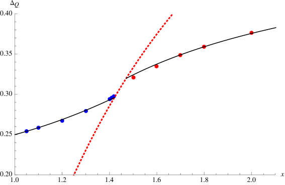
To analyze monopole decoupling in the Veneziano limit, we adopt techniques of [6, Appendix A.3] (see also [34]), which gives the scaling dimension of the quarks/anti-quarks to be
| (43) |
which reduces to
| (44) |
The combined plot of the numerical data points as well as the large expansion of (44) is shown in Figure 2. We find that hits the convergence bound at the critical value .
The analysis in this subsection is partly case-by-case, and it would be interesting to find more uniform patterns in their IR behaviors. A related question is to find a concrete UV Lagrangian description of the theory after decoupling of monopole operators, perhaps along the lines of [35].
3 SQCD
Let us next consider the theory.555Readers not interested in or gauge groups can proceed directly to the discussion of quiver gauge theories in section 6. We find that the structure here is similar to the case of the theory. In particular, we find a small window where the electric and magnetic descriptions hold simultaneously, which window shrinks in the Veneziano limit.
3.1 Dual Pairs
Electric Theory
The electric theory is given by quarks , and comes with a monopole operator . We do not have a superpotential term: . The theory has flavor symmetry, under which the quark and the monopole operator transform as follows:
| (48) |
Magnetic Theory
For , the dual magnetic theory has gauge symmetry with chiral multiplets, dual quark , and additional single chiral multiplets and [21]. Coulomb branch of this magnetic theory is parametrized by the monopole operator .
The charge assignment is given by
| (49) |
The theory also has a superpotential
| (50) |
For , we expect that the magnetic theory is trivial. We propose that the magnetic theory in this case is described by and , with the superpotential
| (51) |
We can verify that this theory is consistent with the charge assignment, which is given as
| (52) |
We have a deformed moduli space for [36], and the supersymmetry is broken for . We therefore concentrate on the case below.
3.2 IR Analysis
Let us parametrize the IR R-symmetry by
| (53) |
where the notation is the same as in the previous section.
Unitarity Bound
The dimensions of the operators and are
| (54) |
The unitary bound is satisfied if
| (55) |
Partition Function
The partition function of the electric theory is given by (see (123) and (124))
| (56) |
For the magnetic theory, we have
| (57) |
for and
| (58) |
for .
Using again the expansion (122), we determine the convergence bound to be
| (59) |
The width of intersection of these two regions shrinks to zero in the Veneziano limit.

-maximization
We can again numerically maximize the -function for small values of and . For this purpose it is sometimes useful to use the trick explained in Appendix E (the same trick could be applied to the theory discussed in the next section). The results of the numerical computation is summarized in Table 2.
|
|
|
|
|
|
|||||||||||
| - |
|
|
|
||||||||||||
| - | - |
|
|
||||||||||||
| - | - | - | |||||||||||||
| - | - | - | - |
For , we always see that the monopole always saturates the unitarity bound, thus we set its scaling dimension at . This modified magnetic theory forces . Inside the table is the only operator which decouples in the IR, and in this sense the structure here is much simpler than that of the SQCD discussed in previous section.
We can again check the consistency with the -theorem by decreasing the values of for a fixed .
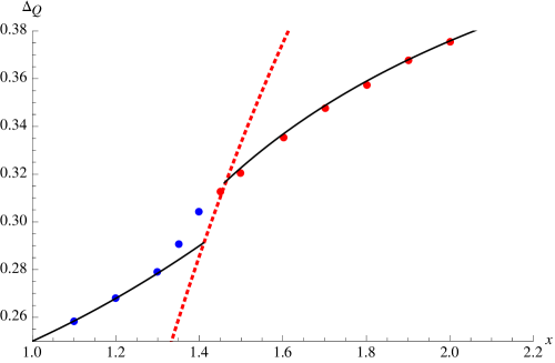
We can also obtain analytic expressions of the scaling dimensions in the large limit, by the techniques of [6, Appendix A.3]. This gives the scaling dimension of the electric quarks to be
| (60) |
In the Veneziano limit, this reduces into
| (61) |
On the other hand, when is close to 1, expansion [6, Appendix A.3] makes sense and we get another expansion of :
| (62) |
In Figure 4 we have plotted these result in combination from the numerical data points coming from the several explicit integrations for small values of and . We find good agreement between numerical and analytical results, and the critical value for is given by .
4 SQCD
Let us now discuss the case of the gauge group. The duality for this case is worked out in [23] (see [28, 37, 38] for a closely related discussion for theories).
It should be kept in mind that the details of the duality depends on the global properties of the gauge group (e.g. or ), as well as the set of local operators we include to the theory. For example, for the gauge group, we have two choices, which are denoted by [23]. In the following we first deal with the case of the gauge group, and then come back to the cases of and gauge groups in section 4.3.
4.1 Dual Pairs
Electric Theory
The electric theory has quarks in the fundamental representation, and as usual we have . The theory also has the monopole operator , the baryon , as well as a composite “baryon-monopole operator” .
The theory has continuous flavor symmetry, under which the fields transform as follows:
| (69) |
Here and represents totally antisymmetric representations. We have listed there discrete symmetry , and (we here list charges only for gauge-invariant fields). We can easily check that is a combination of and , and is not independent. These discrete symmetries will play crucial roles when we change the gauge groups later in section 4.3.
Magnetic Theory
Let us consider the case . First, the magnetic theory has dual quarks . The meson as well as the monopole operator of the electric theory, are now fundamental fields in the magnetic theory. The magnetic theory also has the monopole operator , the baryon , and the dual baryon-monopole .
Note that the baryon and the baryon-monopole do not appear as fundamental fields of the magnetic theory (compare this with the case of theory). Rather they are identified with their magnetic counterparts , by an identification
| (70) |
The magnetic theory has a superpotential
| (71) |
The theory has the same flavor symmetries as the electric theory, under which the fields transform as follows:
| (79) |
Note that the charge assignment for and symmetries here is consistent with the identification (70).
For the case the magnetic theory has no gauge group, contains fields and , with superpotential given by (see [28, 37, 38] for case)
| (80) |
The charge assignment is given by
| (85) |
and as before this case should be treated separately from the rest.
For lower values of , we have the quantum-corrected moduli space for [38], and the supersymmetry is broken for . We will hereafter concentrate on the case .
4.2 IR Analysis
Let us parametrize the IR R-symmetry by
| (86) |
where as before are generators of , respectively.
Unitarity Bound
Let us consider the electric theory. The dimensions of the operators are given by
| (87) | ||||
The unitary bound gives
| (88) | ||||
Notice that in the Veneziano limit, the unitarity bound for the monopole operator depends on the value of , whereas that for the baryon-monopole is independent of .
Partition Function
Let us write down the partition functions of electric and magnetic theories. The precise expression depends on whether is even or odd.
For even with , the electric partition function is given by (see (123) and (124))
| (89) |
while odd with , we have
| (90) |
The magnetic partition function is similar, and for even ()
| (91) |
For with (i.e. ), we have
| (92) |
For (i.e. ), we have
| (93) |
The convergence bounds of the partition functions are given in the following form, which hold irrespective of whether are even or odd:
| (94) |
In this case there is a small overlapping region where both electric and magnetic descriptions are valid. However the width of the overlapping region shrinks to zero in the Veneziano limit. It is therefore expected that we really should not expect both electric and magnetic descriptions to be valid, except for only for limited values of and .

-maximization
We have done the -maximization for several small values of and .666Note that part of the entries have appeared in [37], which gives the critical values of consistent with ours, in the first -maximization. In several cases, however, the monopole operators decouple and we need to do another -maximization, to determine the correct R-symmetry.
|
|
|
|
|
|
|
|||||||||||||
| - |
|
|
|
|
||||||||||||||
| - | - |
|
|
|
||||||||||||||
| - | - | - |
|
|||||||||||||||
| - | - | - | - |
As commented before, one interesting feature of theories is the existence of the baryon-monopole operator . This means that the baryon-monopole , in addition to the baryon , could decouple in the IR. In the examples we studied in Table 3, however, we find that never decouples (this is also the case in the Veneziano limit, to be discussed below, see Figure 6).
We also compute for both odd and even, in the large limit. The partition functions take slightly different forms for odd and even, however it is natural to think that the value of should coincide between the two cases in this limit. Analytic calculation by order in shows that odd/even cases give the same answer, which reads
| (95) |
In the Veneziano limit this expansion reduces to
| (96) |
In the case of the magnetic theory, we can expand in order of which gives us
| (97) |
which reduces in the Veneziano limit into
| (98) |
4.3 , and Gauge Groups
Dual Pairs
Let us now come to the other gauge groups, , and . Note that all these gauge groups have the same Lie algebra as that of . These dualities can be obtained by gauging discrete symmetries of the electric and magnetic theories.
When we gauge a single symmetry, there are three choices: , and , leading to , and theories, respectively, for the electric theory.
We can apply the same gauging to the magnetic theory. In fact, all the terms which appear in the magnetic superpotentials (see (71) and (80)) have charge under any of the three symmetries, and hence the gauging is consistent with the superpotential. There is one big difference from the electric case, however: the role of the and should be exchanged, as follows from the identification (70).
When we gauge two symmetries, there is only one choice, since we are gauging all the discrete symmetries, and we obtain the theory.
These gauging patterns are summarised in Figure 7.
This immediately implies that the correct Aharony-like duality works as [23]
| (99) | ||||
This should be compared with the duality
| (100) |
When we gauge discrete symmetries, we project out the fields which has charge .
For example, when gauging the symmetry (charge conjugation symmetry) we obtain the dualities for gauge groups. In this case, the baryon and the baryon-monopole are projected out, while their combinations, such as and , remain in the theory.
Similarly, when we gauge either or symmetry, the monopole operator in itself is projected out, and we instead have its square remaining:
| (101) |
IR Analysis
We now come to a natural question: does the gauging of the discrete symmetries discussed above have any impact on the IR behavior of the theory?
It turns out most of the preceding analysis for gauge groups does not require any modification. This is because we are primarily interested in -maximization, which requires only the partition function with no operators inserted, and hence is insensitive to gauging of discrete symmetries.
There is one big change, however. While we have the same set of operators, gauging makes some of the gauge-invariant operators gauge-non-invariant. Since the unitarity bound applies only to gauge-invariant operators, the discrete symmetry gauging will in general change the unitarity bounds.
In the analysis for the gauge groups we did not find any examples where the baryon , the meson , or the baryon-monopole decouple. We can therefore concentrate on the monopole operator . As we discussed above, the change for , and gauge groups is that the gauge-invariant monopole operator is not , but rather (101), whose scaling dimension is twice that of .
This immediately means that the unitarity bound for in (88) is replaced by
| (102) | ||||
As expected, the difference from the discrete symmetry gauging goes away in the Veneziano limit.
We can redo the IR decoupling analysis, to obtain the new table as in Table 4. Clearly the only difference can happen when the monopole operator decouples in the theory. In the table this happens when , when the monopole operator no longer decouples.
|
|
|
|
|
|
|
|||||||||||||
| - |
|
|
|
|
|
|||||||||||||
| - | - |
|
|
|
|
|||||||||||||
| - | - | - |
|
|||||||||||||||
| - | - | - | - |
5 Digression on Group Theory
While the analysis in sections 2, 3 and 4 are treated separately, some of the structures are can understood in a more unified manner from the representation theory of the Lie algebras, as one might expect.
To give one example for this phenomena, let us point out that the scaling dimension of the quarks and anti-quarks , in the large expansion up to the order of , can be uniformly represented as
| (103) |
where and are quadratic Casimirs in fundamental and adjoint representation, respectively. Concretely, we have
| (104) | ||||
with which we can verify that (103) reproduce the formulas (43), (60), (95) and (151). We expect the formula (103) to apply to SQCD with other gauge groups, e.g. exceptional gauge groups. That the quadratic Casimirs appear in the expansion coefficients can be explained by the fact that the coefficients compute the certain Feynman diagrams (cf. [6, Appendix B]). Note that in the leading Veneziano limit we always have and the differences of the gauge groups are washed away. This is basically the reason that the plots of (in Figures 2, 4 and 6), as well as the critical value , are similar among different choices of gauge groups with the same ranks.
6 Gauging and Quiver Gauge Theories
The difference between theory and the theory is an example where the gauging of a flavor symmetry dramatically modifies the IR dynamics. We have also seen in section 4.3 that gauging of discrete symmetries also changes the IR decoupling. These can be thought of as particular examples of more general phenomena where the gauging of a flavor symmetry modifies the IR dynamics of the theory.
As yet another example of this type, we study gauging of the flavor symmetry of the SQCD, to obtain a quiver gauge theory with a product gauge group. We discuss the effect of the gauging to the IR R-symmetry, and to the decoupling of monopole operators. Such quiver gauge theories naturally arise in string theory (see e.g [39, 40] and references therein), and (as we will discuss later in the next section) for example in the compactifications of M5-branes.
6.1 Electric Gauging
Let us start with the SQCD with flavors, discussed in section C.
As shown in (129), this theory has symmetry. Let us choose to gauge the diagonal of these two symmetries, which we denote by . The resulting theory then has gauge symmetry, and flavor symmetry, where is the axial (anti-diagonal) combination of . As a result of this gauging, we obtain a quiver gauge theory, whose quiver diagram is shown in Figure 8.
One remark is that the resulting theory has a symmetry exchanging and . In fact, the gauge group can equivalently be taken as , with matters in the bifundamental representations and . This is a quiver gauge theory, and since we only have bifundamental matters the overall of the gauge group trivially decouples, leading to the gauge group as before.
In the rest of this section we use the notation , to make this symmetry more manifest. In fact, now that the symmetry is manifest we can regard the same quiver gauge theory as obtained from the gauging flavor symmetry of the SQCD with flavors, with and reversed from above (Figure 8).
Now, the question we ask in this subsection is whether or not this gauging of the symmetry has any effect in the discussion of the IR scaling dimension and the decoupling of monopole operators.
The best way to see this is to write down the partition function as the parameter corresponding to the mixing of the symmetry, as in Appendix C:
| (105) |
Note that the integral is kept invariant under the simultaneous shift of and , and this represents the overall decoupled commented before. The same partition function can also be written as
| (106) |
In either way, it is clear that gauging dramatically change the partition function as a function of the parameter , and consequently the IR R-charges/conformal dimensions of the theory. In fact, this is to be expected since we have a manifest symmetry between and after gauging; by contrast theory and clearly have different IR dynamics, as we have seen in the rest of this paper.
This symmetry between and is actually a source for trouble, when we consider the convergence bound for the electric partition function. The convergence bound before gauging was worked out in (34), and since now we have symmetry and and , we should impose the same constraint with and ( and ) exchanges. This gives
| (107) |
and in particular will be negative unless .
Note that convergence constraint is ameliorated by including flavor matters to gauge groups and . Suppose that we include flavors ( flavors) to gauge groups and . The convergence constraint then reads
| (108) |
and in particular the constraint in practice goes away for sufficiently large and . Such flavors are natural from string theory constructions, however we will set in the discussion below, to simplify analysis.
6.2 Magnetic Gauging
To avoid this convergence issue, one might be tempted to switch to the magnetic description. Namely, instead of gauging the flavor symmetry of the electric theory, we can choose to gauge the flavor symmetry of the magnetic theory.
For the case , we can first go to the magnetic theory of SQCD with flavors, go to the magnetic dual, and then gauge the flavor symmetry of the theory. Note that these magnetic descriptions break the symmetry between and , as is clear from the fact that the magnetic descriptions requires us to take . The resulting partition function is given by (compare this with (32)):
| (109) |
Equivalently, we can start with the SQCD with flavors, and then gauge the flavor symmetry (compare (148)):
| (110) |
The formal equivalence of the two expressions (109) and (110) (up to a constant phase factor) can be checked directly by using the identities (158) and (121). (In fact, this is essentially the argument used for deriving dualities from dualities, as reviewed in Appendix D).
Unfortunately, the convergence bound for (109) and (110) is satisfied for
| (111) | ||||
where the first (second) inequality comes from the convergence of the () integrals. In other words the partition function (109) and (110) cannot be used for any practical -maximization.
The situation is better for the case . We can then gauge the flavor symmetry of the magnetic theory, leading to the partition function
| (112) | ||||
We can instead choose to gauge the flavor symmetry of the magnetic theory, leading to the expression
| (113) | ||||
The equivalence of (112) and (113) can again be checked by using the identities (158) and (121). The convergence bound for these expressions is an inequality
| (114) |
It is natural to expect that the magnetic quiver theories discussed here are dual to the electric quiver gauge theories discussed before. There is one caveat, however. We have implicitly assumed that the order of two operations, namely gauging of the flavor symmetry and going to the dual magnetic description, commute with each other. Since the duality at hand is an IR duality, in general the gauging of the flavor symmetry could change the behavior under the RG flow, and hence spoil the IR duality.
We however expect that this does not happen when the gauge coupling for the newly-gauged flavor symmetry is much smaller than other gauge couplings. If in the UV the gauge coupling for is much larger than that for the gauge group, one imagines that the strong coupling effect of kicks in first, and then the dynamics of does not matter until at much lower scales. We can then discuss the dynamics of and gauge groups separately. Since the partition function is independent of gauge couplings, the equality of the partition functions should hold for any value of the gauge coupling, giving further evidence for the duality after gauging.
Numerical Results
The numerical analysis of the quiver case is computationally more challenging than the SQCD case, and as we have seen the convergence bound tends to be severe. Therefore let us here consider the simplest case of magnetic theory. We can then do -maximization for the partition function (112) (compare with Table 1). The numerical results for the values are summarized in Table 5.
There are two remarks on this result. First, the value of at the maximum is different from that before gauging, as expected. Another non-trivial result here is that here in none of these cases exhibit operator decoupling. This is partly because the meson of the magnetic theory, after gauging, is now an adjoint field with respect to the newly-introduced gauge symmetry, and hence is not gauge invariant. Therefore there is no need to consider the unitarity bound of the meson itself.
|
|
|
|
|
6.3 General Quivers
Having discussed quiver gauge theories with two nodes, we can discuss more general 3d quiver gauge theories, whose matter content is determined by a quiver diagram, i.e. an oriented graph777We also need to specify the superpotentials, however this choice does not really modify the qualitative features of the conclusions below.. We can then gauge the appropriate flavor symmetries, whose effect is to concatenate two quiver diagrams and to generate a more complicated quiver diagram (Figure 9). For example, if we glue two quivers at a node to obtain a new quiver , then partition function for the larger quiver can be schematically written in the form
| (115) |
where is the contribution from the vector multiplet which is gauged under the gluing, and denote the parameters repressing the flavor symmetries of the theories .

As before, the extremum of as a function of () is in general different from that of the (). This means that to tell whether the monopole operator for the gauge group in the quiver decouples or not, we need to know in advance the detailed data for the quiver , however large the quiver may be.888In the spirit of [41] one might be tempted to say that there is a “long-range entanglement in the theory space”. It would be interesting to explore this point further, and connect the discussion here to the entanglement in the dual statistical mechanical model discussed in [42, 43]. This is in sharp contrast with the case of 3d supersymmetry, where the IR decoupling of the monopole operators can be checked locally at the quiver diagram, by verifying the inequality (cf. [44, 45] for recent discussion in gravity dual).
7 Implications for M5-brane Compactifications
The comments from the previous section has interesting implications to the M5-brane compactifications, which we now turn to.
7.1 Boundary Conditions of 4d SYM
Let us first start with the results of [14], which classifies –BPS boundary conditions of 4d Super Yang-Mills Theory (SYM). Some of the boundary conditions (of the Neumann type, realized by D3-branes ending on NS5-branes in type IIB string theory) contain a non-trivial boundary field theory , which is given as a 3d linear-chain quiver gauge theory. When contains monopole operators decoupling in the IR, we regard the corresponding as containing redundant degrees of freedom, in the sense that contains fields which decouples completely from the bulk 4d theory. Since we are interested in the classification of the minimal set of boundary conditions in the IR, this means we can disregard such from the classification of boundary conditions. This, together with the criterion mentioned above, lead to the conclusion that the choices of are exhausted by the so-called theories, with being the partition of .999 If we consider the mixture of Dirichlet and Neumann boundary conditions we obtain a slightly more general class of theories , labeled by a pair of partitions .
We can now consider the –BPS boundary conditions [46, 47], whose boundary field theory would then be 3d theories. As we have seen above the criterion for the decoupling/un-decoupling is now more complicated than the inequality . In particular, in the Veneziano limit101010 This is natural in the context of the holographic dual. we have learned from [6] that the decoupling happens at the critical value . This suggests that the minimal set of (Neumann type) boundary conditions should no longer be labeled by partitions.111111 In 3d theories, for each vertex of the quiver diagram we have the choice of whether or not to include adjoint chiral multiplet. This means that the natural generalization of the –BPS analysis is that the boundary conditions are labeled by a decorated partition. However, our point here is that this is likely a redundant characterization of the IR boundary condition. It would be interesting to see if/how this conclusion could fit together with the analysis of the generalized Nahm equations in [46, 47], or their 4d counterparts [48, 49].
7.2 Co-dimension Defects of 6d Theory
Since the 4d SYM is an compactification of 5d SYM (super-Yang-Mills) and also a compactification of the 6d theory of type, we can try to lift the conclusions of the previous subsection into the statements on the 5d SYM and the 6d theory.
For the -BPS case, the same consideration leads to the conclusion that (see [50, section 2.1] for review) the –BPS co-dimension 2 defects are labeled by a partition of , and the effect of the defect in the 5d language is to couple the 5d SYM to the theory mentioned above. This fact has been utilized recently in the context of the compactifications of the 6d theories on 2-manifolds [51, 52, 53] and 3-manifolds [54, 50].
Now we can repeat the same argument for the –BPS boundary conditions, and again obtain –BPS boundary conditions for 5d SYM and the 6d theory. Our conclusion is then that these defects should not be labeled by partitions, since otherwise we would be over-counting. This should have some interesting counterparts as data specifying –BPS defects in 4d theories arising from the 2-manifold compactifications [55, 56], or 3d theories arising from the 3-manifold compactifications [57, 58, 59, 60].
Acknowledgements
We would like to thank I. Klebanov for encouragement, advice and for careful readings of this manuscript. We also thank I. Yaakov and B. Willett for discussion. J. L. received support from the Samsung Scholarship. M. Y. was supported by WPI program (MEXT, Japan), by JSPS Program for Advancing Strategic International Networks to Accelerate the Circulation of Talented Researchers, by JSPS KAKENHI Grant No. 15K17634, and by Institute for Advanced Study.
Appendix A Monopole Operators
Given a root of the gauge group, we can write down the corresponding monopole operator
| (116) |
where are the Cartan part of the scalar in the adjoint vector multiplet, and are the dual photon of the Cartan part of the gauge group. The latter is periodic with period , making well-defined.
Only the ’s for positive simple roots are independent, and hence classically we have independent monopole operators. This parametrizes the classical Coulomb branch. However many of these Coulomb branches are lifted by quantum corrections (instanton-generated superpotential).
For example, for , classically we have monopole operators
| (117) |
however the only remaining operator in the end is
| (118) |
This is the monopole operator discussed in section 2.
Appendix B Partition Functions
The partition function [16, 15, 17] is given by (in the absence of Chern-Simons terms, FI parameters and real mass parameters)
| (119) |
where is the order of the Weyl group, () is the representation under the gauge group (R-charge) of the chiral multiplet and the function is defined by
| (120) |
This function has poles at integers on the real axis, except at the origin. We also have the relation
| (121) |
For convergence of the partition function we use the following asymptotics in the limit :
| (122) |
For gauge groups the Cartan subalgebra is parametrized as
| (123) |
and the roots are given by
| (124) |
Appendix C SQCD
In this Appendix we briefly summarize the case of the gauge group [6]. It is instructive to compare the discussion in this Appendix with that of the theory in the main text. Some of the ingredients discussed in this Appendix will be used in the discussion of quiver gauge theories in section 6.
C.1 Dual Pairs
Electric Theory
The electric theory is similar to the SQCD. The major difference is that we have two remaining monopole operators .
The theory has a gauge symmetry, as well as flavor symmetries, under which the fields transform as follows:
| (129) |
Note that compared with the case we have the topological symmetry in this case, whereas the symmetry, being part of the gauge symmetry, is absent.
Magnetic Theory
Let us first assume . The magnetic theory has gauge group (remember the definition ), and has dual quark , anti-quarks , and the meson and . The magnetic theory also has two monopole operators for the dual photons of magnetic gauge groups. The superpotential is given by
| (130) |
The theory again has the same flavor symmetry as the electric theory, under which the fields transform as follows:
| (137) |
For , the magnetic theory do not have a gauge group, and is described by the chiral superfields , with the superpotential
| (138) |
The charge assignment in this case is
| (142) |
C.2 IR Analysis
As in other cases discussed in the main text, we need to consider the IR-mixing of the R-symmetry with the symmetry
| (143) |
Note that we do not need to consider the mixing with the topological symmetry, since otherwise the parity is broken.
Unitarity Bound
The dimensions of and are given by
| (144) |
which leads to the unitarity bound is given by
| (145) |
which in the Veneziano limit simplifies to
| (146) |
Note this requires , and we will find the crack before this value.
Partition Function
The partition function of the electric theory is given by
| (147) |
and that of the magnetic theory (for ) by
| (148) |
The convergence of the expression for the partition function above gives
| (149) |
As explained in the main text for the case, we can either derive this from the positivity of the dimension of the monopole operators, or from the positivity of the effective FI parameter introduced in (37):
| (150) |

The large and small expansions of the scaling dimensions of the matter quarks are given by
| (151) |
and
| (152) |
Appendix D Dualities from Dualities
In this Appendix we derive the dualities from the dualities. The basic argument is not really new, and basically the same as in [24], except that here we work out the derivation at the level of the partition function (as opposed to the 3d index in [24]). Similar manipulations appear in the discussion of quiver gauge theories in section 6.
Let us begin with the partition functions of theories, with all the real mass/FI parameters to our partition functions turned on in (147), (148) (this means that is now complexified). When we denote the real mass parameters for the and symmetries by (), we have the partition functions
| (153) |
and
| (154) |
Now to obtain the duality all we need to do is apply the -transformation (as defined in [61]) to the global symmetry. In other words we add an off-diagonal Chern-Simons term
| (155) |
and gauge the gauge field for . As we will see momentarily, the new gauge field will be identified with that of the symmetry of the magnetic theory: at the level of the partition function this amounts to the Fourier transform with respect to .
For the electric theory, we have
| (156) |
where in the last line we shifted . We can check that this gives the charge assignment of the electric theory, and in particular that this answer gives the (29) when we take and when we identify .121212The factor of here is explained from the fact that the partition function depends on a complex combination, the real part being the anomalous dimension due to the mixing with a global symmetry and the imaginary part being the real mass [15, 29]. Note also that in the Fourier transform we have included a factor of ; this was chosen such that the parameter after the Fourier transform can be directly identified with the real mass parameter for the symmetry.
We can add the same off-diagonal Chern-Simons term (155) to the magnetic theory, whose partition function is
| (157) |
However this is not yet the magnetic theory discussed in the body of the text. We further need to use the duality for the theory. The magnetic theory is given in (138), where is now a matrix (a number): . At the partition function level this gives the following equality (which holds up to an overall constant term), which is a specialization of the pentagon identity for quantum dilogarithm:
| (158) |
After applying (158)131313we take in (158)., the expression (157) becomes
| (159) |
Again, if we set this coincides with the magnetic partition function (32) we wrote down in the main text, under the identification .
We discussed above the case of , however the case of is similar and simpler, so we will not repeat here.
Appendix E Numerical Tricks
The evaluation of the our partition function requires a multi-dimensional integral whose integrands oscillates relatively quickly. In some cases, we find it numerically more advantageous to convert the multi-dimensional integral into a sum of a product of one-dimensional integrals. Let us illustrate this for the case of SQCD: the same strategy works in a similar manner for and SQCD.
The trick is to use the Weyl character formula
| (160) |
where is the Weyl vector and is the Weyl group (-th symmetric group).
References
- [1] O. Aharony, A. Hanany, K. A. Intriligator, N. Seiberg and M. Strassler, “Aspects of N=2 supersymmetric gauge theories in three-dimensions”, Nucl. Phys. B499, 67 (1997), hep-th/9703110.
- [2] J. de Boer, K. Hori and Y. Oz, “Dynamics of N=2 supersymmetric gauge theories in three-dimensions”, Nucl. Phys. B500, 163 (1997), hep-th/9703100.
- [3] I. Affleck, J. A. Harvey and E. Witten, “Instantons and (Super)Symmetry Breaking in (2+1)-Dimensions”, Nucl. Phys. B206, 413 (1982).
- [4] D. Kutasov, “A Comment on duality in N=1 supersymmetric nonAbelian gauge theories”, Phys. Lett. B351, 230 (1995), hep-th/9503086.
- [5] D. Kutasov and A. Schwimmer, “On duality in supersymmetric Yang-Mills theory”, Phys. Lett. B354, 315 (1995), hep-th/9505004.
- [6] B. R. Safdi, I. R. Klebanov and J. Lee, “A Crack in the Conformal Window”, JHEP 1304, 165 (2013), arxiv:1212.4502.
- [7] G. Mack, “All Unitary Ray Representations of the Conformal Group SU(2,2) with Positive Energy”, Commun. Math. Phys. 55, 1 (1977).
- [8] M. Flato and C. Fronsdal, “Representations of Conformal Supersymmetry”, Lett. Math. Phys. 8, 159 (1984).
- [9] V. K. Dobrev and V. B. Petkova, “All Positive Energy Unitary Irreducible Representations of Extended Conformal Supersymmetry”, Phys. Lett. B162, 127 (1985).
- [10] S. Minwalla, “Restrictions imposed by superconformal invariance on quantum field theories”, Adv. Theor. Math. Phys. 2, 781 (1998), hep-th/9712074.
- [11] J. Penedones, E. Trevisani and M. Yamazaki, “Recursion Relations for Conformal Blocks”, arxiv:1509.00428.
- [12] M. Yamazaki, “Comments on Determinant Formulas for General CFTs”, arxiv:1601.04072.
- [13] V. Borokhov, A. Kapustin and X.-k. Wu, “Monopole operators and mirror symmetry in three-dimensions”, JHEP 0212, 044 (2002), hep-th/0207074.
- [14] D. Gaiotto and E. Witten, “S-Duality of Boundary Conditions In N=4 Super Yang-Mills Theory”, Adv. Theor. Math. Phys. 13, 721 (2009), arxiv:0807.3720.
- [15] D. L. Jafferis, “The Exact Superconformal R-Symmetry Extremizes Z”, JHEP 1205, 159 (2012), arxiv:1012.3210.
- [16] A. Kapustin, B. Willett and I. Yaakov, “Exact Results for Wilson Loops in Superconformal Chern-Simons Theories with Matter”, JHEP 1003, 089 (2010), arxiv:0909.4559.
- [17] N. Hama, K. Hosomichi and S. Lee, “Notes on SUSY Gauge Theories on Three-Sphere”, JHEP 1103, 127 (2011), arxiv:1012.3512.
- [18] V. Niarchos, “Comments on F-maximization and R-symmetry in 3D SCFTs”, J. Phys. A44, 305404 (2011), arxiv:1103.5909.
- [19] T. Morita and V. Niarchos, “F-theorem, duality and SUSY breaking in one-adjoint Chern-Simons-Matter theories”, Nucl. Phys. B858, 84 (2012), arxiv:1108.4963.
- [20] P. Agarwal, A. Amariti and M. Siani, “Refined Checks and Exact Dualities in Three Dimensions”, JHEP 1210, 178 (2012), arxiv:1205.6798.
- [21] O. Aharony, “IR duality in d = 3 N=2 supersymmetric USp(2N(c)) and U(N(c)) gauge theories”, Phys. Lett. B404, 71 (1997), hep-th/9703215.
- [22] O. Aharony, S. S. Razamat, N. Seiberg and B. Willett, “3d dualities from 4d dualities”, JHEP 1307, 149 (2013), arxiv:1305.3924.
- [23] O. Aharony, S. S. Razamat, N. Seiberg and B. Willett, “3 dualities from 4 dualities for orthogonal groups”, JHEP 1308, 099 (2013), arxiv:1307.0511.
- [24] J. Park and K.-J. Park, “Seiberg-like Dualities for 3d N=2 Theories with SU(N) gauge group”, arxiv:1305.6280.
- [25] F. A. H. Dolan, V. P. Spiridonov and G. S. Vartanov, “From 4d superconformal indices to 3d partition functions”, Phys. Lett. B704, 234 (2011), arxiv:1104.1787.
- [26] B. Willett and I. Yaakov, “N=2 Dualities and Z Extremization in Three Dimensions”, arxiv:1104.0487.
- [27] D. Bashkirov, “Aharony duality and monopole operators in three dimensions”, arxiv:1106.4110.
- [28] F. Benini, C. Closset and S. Cremonesi, “Comments on 3d Seiberg-like dualities”, JHEP 1110, 075 (2011), arxiv:1108.5373.
- [29] G. Festuccia and N. Seiberg, “Rigid Supersymmetric Theories in Curved Superspace”, JHEP 1106, 114 (2011), arxiv:1105.0689.
- [30] R. C. Myers and A. Sinha, “Seeing a c-theorem with holography”, Phys. Rev. D82, 046006 (2010), arxiv:1006.1263.
- [31] D. L. Jafferis, I. R. Klebanov, S. S. Pufu and B. R. Safdi, “Towards the F-Theorem: N=2 Field Theories on the Three-Sphere”, JHEP 1106, 102 (2011), arxiv:1103.1181.
- [32] I. R. Klebanov, S. S. Pufu and B. R. Safdi, “F-Theorem without Supersymmetry”, JHEP 1110, 038 (2011), arxiv:1105.4598.
- [33] H. Casini and M. Huerta, “On the RG running of the entanglement entropy of a circle”, Phys. Rev. D85, 125016 (2012), arxiv:1202.5650.
- [34] I. R. Klebanov, S. S. Pufu, S. Sachdev and B. R. Safdi, “Entanglement Entropy of 3-d Conformal Gauge Theories with Many Flavors”, JHEP 1205, 036 (2012), arxiv:1112.5342.
- [35] I. Yaakov, “Redeeming Bad Theories”, JHEP 1311, 189 (2013), arxiv:1303.2769.
- [36] A. Karch, “Seiberg duality in three-dimensions”, Phys. Lett. B405, 79 (1997), hep-th/9703172.
- [37] C. Hwang, K.-J. Park and J. Park, “Evidence for Aharony duality for orthogonal gauge groups”, JHEP 1111, 011 (2011), arxiv:1109.2828.
- [38] O. Aharony and I. Shamir, “On supersymmetric QCD Theories”, JHEP 1112, 043 (2011), arxiv:1109.5081.
- [39] Y.-H. He, “On algebraic singularities, finite graphs and D-brane gauge theories: A String theoretic perspective”, hep-th/0209230.
- [40] M. Yamazaki, “Brane Tilings and Their Applications”, Fortsch. Phys. 56, 555 (2008), arxiv:0803.4474.
- [41] M. Yamazaki, “Entanglement in Theory Space”, Europhys. Lett. 103, 21002 (2013), arxiv:1304.0762.
- [42] M. Yamazaki, “Quivers, YBE and 3-manifolds”, JHEP 1205, 147 (2012), arxiv:1203.5784.
- [43] Y. Terashima and M. Yamazaki, “Emergent 3-manifolds from 4d Superconformal Indices”, Phys. Rev. Lett. 109, 091602 (2012), arxiv:1203.5792.
- [44] W. Cottrell, J. Hanson and A. Hashimoto, “Dynamics of supersymmetric field theories in 2+1 dimensions and their gravity dual”, arxiv:1509.04749.
- [45] W. Cottrell and A. Hashimoto, “Resolved gravity duals of quiver field theories in 2+1 dimensions”, arxiv:1602.04765.
- [46] A. Hashimoto, P. Ouyang and M. Yamazaki, “Boundaries and defects of SYM with 4 supercharges. Part I: Boundary/junction conditions”, JHEP 1410, 107 (2014), arxiv:1404.5527.
- [47] A. Hashimoto, P. Ouyang and M. Yamazaki, “Boundaries and defects of SYM with 4 supercharges. Part II: Brane constructions and 3d field theories”, JHEP 1410, 108 (2014), arxiv:1406.5501.
- [48] G. Bonelli, S. Giacomelli, K. Maruyoshi and A. Tanzini, “N=1 Geometries via M-theory”, JHEP 1310, 227 (2013), arxiv:1307.7703.
- [49] D. Xie, “M5 brane and four dimensional N = 1 theories I”, JHEP 1404, 154 (2014), arxiv:1307.5877.
- [50] D. Gang, N. Kim, M. Romo and M. Yamazaki, “Aspects of Defects in 3d-3d Correspondence”, arxiv:1510.05011.
- [51] K. Yonekura, “Supersymmetric gauge theory, (2,0) theory and twisted 5d Super-Yang-Mills”, JHEP 1401, 142 (2014), arxiv:1310.7943.
- [52] M. Bullimore and H.-C. Kim, “The Superconformal Index of the (2,0) Theory with Defects”, JHEP 1505, 048 (2015), arxiv:1412.3872.
- [53] M. Bullimore, H.-C. Kim and P. Koroteev, “Defects and Quantum Seiberg-Witten Geometry”, JHEP 1505, 095 (2015), arxiv:1412.6081.
- [54] D. Gang, N. Kim, M. Romo and M. Yamazaki, “Taming Supersymmetric Defects in 3d-3d Correspondence”, arxiv:1510.03884.
- [55] D. Gaiotto, “N=2 dualities”, JHEP 1208, 034 (2012), arxiv:0904.2715.
- [56] N. Wyllard, “A(N-1) conformal Toda field theory correlation functions from conformal N = 2 SU(N) quiver gauge theories”, JHEP 0911, 002 (2009), arxiv:0907.2189.
- [57] Y. Terashima and M. Yamazaki, “SL(2,R) Chern-Simons, Liouville, and Gauge Theory on Duality Walls”, JHEP 1108, 135 (2011), arxiv:1103.5748.
- [58] T. Dimofte, D. Gaiotto and S. Gukov, “Gauge Theories Labelled by Three-Manifolds”, Commun. Math. Phys. 325, 367 (2014), arxiv:1108.4389.
- [59] S. Lee and M. Yamazaki, “3d Chern-Simons Theory from M5-branes”, JHEP 1312, 035 (2013), arxiv:1305.2429.
- [60] C. Cordova and D. L. Jafferis, “Complex Chern-Simons from M5-branes on the Squashed Three-Sphere”, arxiv:1305.2891.
- [61] E. Witten, “SL(2,Z) action on three-dimensional conformal field theories with Abelian symmetry”, hep-th/0307041.