Discriminating Topology in Galaxy Distributions using Network Analysis

Abstract

The large-scale distribution of galaxies is generally analyzed using the two-point correlation function. However, this statistic does not capture the topology of the distribution, and it is necessary to resort to higher order correlations to break degeneracies. We demonstrate that an alternate approach using network analysis can discriminate between topologically different distributions that have similar two-point correlations. We investigate two galaxy point distributions, one produced by a cosmological simulation and the other by a Lévy walk, that have different topologies but yield the same power-law two-point correlation function. For the cosmological simulation, we adopt the redshift $z=0.58$ slice from Illustris (Vogelsberger et al. 2014A) and select galaxies with stellar masses greater than $10^{8}$$M_{\odot}$. The two point correlation function of these simulated galaxies follows a single power-law, $\xi(r)\sim r^{-1.5}$. Then, we generate Lévy walks matching the correlation function and abundance with the simulated galaxies. We find that, while the two simulated galaxy point distributions have the same abundance and two point correlation function, their spatial distributions are very different; most prominently, filamentary structures, which are present in the simulation are absent in Lévy fractals. To quantify these missing topologies, we adopt network analysis tools and measure diameter, giant component, and transitivity from networks built by a conventional friends-of-friends recipe with various linking lengths. Unlike the abundance and two point correlation function, these network quantities reveal a clear separation between the two simulated distributions; therefore, the galaxy distribution simulated by Illustris is not a Lévy fractal quantitatively. We find that the described network quantities offer an efficient tool for discriminating topologies and for comparing observed and theoretical distributions.

I. Introduction

Throughout the history of the Universe, various geometrical and topological features have formed, evolved, and vanished in the cosmic energy and matter distribution. It is undeniably critical to quantify and measure such features, since many of them can provide definitive probes for constraining important cosmological parameters.

During the past two decades, studies of anisotropic features in the cosmic microwave background (CMB), specifically acoustic peaks, have motivated the so-called $\Lambda$ cold dark matter ($\Lambda$CDM) cosmology as a standard paradigm (e.g., Hinshaw et al. 2013, Aghanim et al. 2015) and made a new step forward in precision cosmology. Various experiments (Levi et al. 2013, Delubac et al. 2015, Zhao et al. 2015), currently beginning or underway, are mapping out the expansion history of the Universe with unprecedented accuracy, by measuring baryon acoustic oscillations (BAO). These experiments will also result in the most detailed maps of the large-scale galaxy distribution over a wide range in redshifts, from $z\sim 0$ to $z\sim 3$.

The successes of measuring CMB acoustic peaks and BAO features demonstrate how important the two-point correlation functions (or power spectra) are for quantifying cosmic structures. Higher order $n-$point correlation statistics are essential for analyzing cosmic structures. For example, the three and four point correlation functions (or, bi- and tri-spectra) can constrain the non-Gaussianity of primordial quantum fluctuations (Barkats et al. 2014, Ade et al. 2015); however, these measures are computationally challenging (e.g., Kulkarni et al. 2007, Gil-Marín et al. 2015).

Along with the successful $n-$point statistics, many topological measurements have been introduced, such as genus numbers and Minkowski functionals (Gott, Weinberg & Melott 1987, Eriksen et al. 2004). To identify voids and filaments, various methods have been adapted from other fields of science, including minimum-spanning trees, watersheds, Morse theory, wavelets, and smoothed Hessian matrices (e.g., Barrow, Bhavsar & Sonoda 1985, Sheth et al. 2003, Martínez et al. 2005, Aragón-Calvo et al. 2007, Colberg 2007, Sousbie et al. 2008, Bond, Strauss & Cen 2010, Lidz et al. 2010, Cautun et al. 2013). While these topological diagnostics have provided important insights into the nature of structure in the Universe, this wide but heterogeneous range of applied methodologies reflects how difficult it is to find a consistent and comprehensive framework for quantifying and measuring the topology of the Universe, in contrast to the successful $n-$point statistics.

Many of these studies generate a continuous density field by smoothing the galaxy point distribution and then measuring geometric topologies of genus numbers and Minkowski functionals. Our approach, which we term “network cosmology”, is to characterize the topology of the discrete point distribution directly using graph theory and network algorithms.

As a pilot study to explore new ways to quantify cosmic topologies, Hong & Dey (2015; hereafter, HD15) applied the analysis tools developed for the study of complex networks (e.g. Albert & Barabási 2002, Newman 2010) to the study of the large-scale galaxy distribution. The basic idea is to generate a graph (i.e., a “network”) composed of vertices (nodes) and edges (links) from a galaxy distribution, and then measure network quantities used in graph theory. In this paper, we demonstrate the utility of these techniques for differentiating between point distributions that have identical two-point correlations but different spatial distributions and topologies.

Our paper is organized as follows. In §2, as a more specific introduction to this paper, we offer a general discussion about what types of features can be measured from galaxy survey data, the strong and weak points of $n-$point statistics, and how network representations of galaxy distributions can improve our ability to quantify topological features in the Universe. In §3, we describe our samples to be investigated, the snapshot of Illustris data (Vogelsberger et al. 2014A) and Lévy walks with various parameters. In §4, we present the two-point correlation functions and network measurements from the samples and discuss the results. Then, we summarize in §5.

II. Geometric Configurations vs. Topological Textures in Galaxy Surveys

Sections 2.1 and 2.2 present the definitions of geometry and topology used in this paper and our overall philosophy in applying methods of network analyses to galaxy distributions. Readers can skip these sections without losing the main thread of this paper.

II.1. Geometry vs. Topology

The terms geometry and topoplogy are often used interchangeably in astronomical contexts. Geometry can be defined as the study of shapes of known metric dimensions, whereas topology refers to the intrinsic shape properties that are invariant to deformation (i.e., homotopic). For example, triangles are 3-sided geometric shapes that are characterized by the measures of their angles and sides. However, removing all metric features from triangles, we can also represent them topologically as a metric-free structure with three vertices where each vertext is connected to the other two by two edges. Another well-known example is the comparison between a mug and a donut; these are different geometric shapes with a common topology, the latter measured by a zero genus number.

Euler characteristics in graphs or genus numbers in manifolds are mathematically well-defined topological measures, invariant under homotopy or homeomorphism. However, most practical measurements are both geometric and topological, and do not have to be homotopy invariant in the strict mathematical sense in order to be topologically meaningful. For example, the set of Roman alphabets is topological. We can consistently recognize letters irrespective of font or handwriting since each alphabet has its own distinct topology. “i”, “k”, “l” are topologically very different even in mathematically rigorous measures. However, “i” and “j” are indistinct topologically. They are discerned instead by the differences in length and curve (angle). The process of reading, i.e., visually measuring the characteristics of each letter, is predominantly topological but includes geometric aspects.

In galaxy surveys, $n-$point statistics are typical measurements, as presented in §1. These are geometrically driven measurements; $n-$point correlation functions contain specific information about distances and angles between galaxies. From a practical standpoint, this renders $n-$point statistics computationally challenging, since computation times are dominated by the handling of geometric information.

If we are only interested in topological features, much of the geometric information is redundant. For example, if we need to count all triangles in a friends-of-friends network from a certain galaxy distribution, we can run a network algorithm to count all triangular subgraphs. We do not need to measure the three point statistic for the problem of only counting triangles. Likewise, if we are interested in the number of holes for an object, we do not need to know whether it looks like a mug or a donut.

Therefore, in practical analyses, we need to determine whether we are interested in quantifying geometric configurations or topological textures, when extracting measurements from galaxy survey data. Theoretically, a complete set of $n-$point statistics can suffice to characterize all aspects of a point distribution. However, such geometric analyses can be very inefficient when our prime focus is to quantify topological textures of the Universe.

II.2. Continuous Density Function vs. Discrete Point Distribution

To quantify topological structures of the Universe, many conventional studies have used geometric topology, where a metric topology is well-defined in a continuous cosmic matter distribution, $\rho(x)$, or its density contrast, $\delta(x)$. In this approach, discrete observables such as galaxy or halo distributions, $n(x)$, are considered as biased samplings of the underlying continuous cosmic matter distribution. Therefore, we generally smooth this discrete point distribution to approximate the continuous mass field.

In a different and empirical approach, we do not smooth over the discrete observable, $n(x)$. Instead, we build a network structure (or, a graph) from this discrete observable, and measure network quantities; hence, algebraic topology from discrete observables, contrast to the previous approach of metric topology from continuous observables. Hereafter, we refer to the former as “DA” (discrete and algebraic) approach, and the latter as “CM” (continuous and metric) approach.

The CM and DA approaches differ in methodology. The CM approach is based on differential geometry and topology; hence, parameters of geometric shape and topology are derived from differentials or integrals of the density field. For example, the Hessian matrix is derived from partial differentials of the density field. From the eigenvalues of this matrix, the clusters, walls, and filaments of the density field are classified (Aragón-Calvo et al. 2007, Bond et al. 2010, Cautun et al. 2013). Minkowski functionals are defined using integrals of the density field to quantify geometric and topological features such as area, perimeter, and genus (Mecke et al. 1994, Park et al. 2005, Hikage et al. 2008, Ducout et al. 2013).

On the other hand, our DA approach (which we refer to as “network cosmology”) mostly utilizes network algorithms developed and used in computer science, mathematics, physics, and sociology. With its roots in Euler’s brilliant solution to the Königsburg bridge problem (Euler 1741), network science has grown rapidly during the last two decades, driven by the growth of computing power, large databases, and internet infrastructures (Albert & Barabási 2002, Barabási 2009, Newman 2010). Networks can be constructed for studying subjects as diverse as the relationships between costarring actors, protein interactions, paper citations, the food web, power grids, traffic patterns, the world wide web (WWW), etc. Many network tools have been developed to extract useful information from these various kinds of big data networks. We have attempted, therefore, to utilize these network tools for investigating galaxy survey data. For example, PageRank was developed for prioritizing the importance of WWW documents, used in the search engine, Google (Page et al. 1999). We can measure these PageRanks for galaxies, once we build a galaxy network from galaxy survey data. As we have a friend recommendation from Facebook, such a recommendation algorithm also can be applied to our galaxy network. This is the basic philosophy of our network cosmology.

Early attempts of applying network science tools to galaxy point distributions made use of percolation methods and the minimum spanning tree, or MST (see, e.g, Shandarin et al. 1983AB, Barrow et al. 1985, Colberg 2007). Since these pioneering papers, the tools developed for analyzing networks have proliferated and mathematically matured. Our earlier work, HD15, investigated galaxy distributions using various measures of network centrality (degree, betweenness, and closeness). In this paper, we apply the network measures of diameter, giant component fraction, and transitivity to simulated galaxy point distributions.

II.3. Degeneracy in Two-point Correlation Function

It has long been reported that observed galaxy populations exhibit single power-law clusterings within several tens of megaparsecs in comoving scale (e.g., Davis & Peebles 1983, Shandarin & Zeldovich 1989, Adelberger et al. 2005). Within the cold dark matter paradigm of galaxy formation, galaxies are biased tracers of the underlying matter distribution and the clustering properties of different galaxy populations can be diverse, depending on how galaxies populate their dark matter halos. Analysis of the two-point correlation function of different galaxy populations has resulted in the idea of the “halo occupation distribution”; i.e., the probability that a given halo contains a certain number of galaxies, and has given rise to various analytic and probabilistic formulations of this function (Berlind & Weinberg 2002, Zheng et al. 2005, Tinker 2007). From these halo occupation studies, there should be a transitioning scale from the dominance of the one halo term to the two halo term; hence there is no need for galaxies to show a single, seamless power-law clustering trend. The apparent single power-law behavior, especially for low redshift galaxies, is thought to be due to massive galaxy clusters whose contribution erases the transition feature (Berlind & Weinberg 2002).

For a single power-law correlation, a couple of methods have been proposed to generate mock galaxies including Lévy walks (Mandelbrot 1975) and multi-layered shells akin to Russian dolls or onion rings (Soneira & Peebles 1978; hereafter, SP78). These models are “statistical”, since, unlike galaxies in simulations or the real Universe, their clustering properties do not originate from “gravitational” interaction, but instead from a statistical fractal realization. These models can be tuned to match both the abundance and the two-point correlation function of the observed galaxy distribution.

Now, we raise two questions:

(1) What is the gap between gravitational and statistical realizations?, and

(2) Can we quantify the gap to finally test how much statistical models are reliable as mocks?

These are based on doubts about the sufficiency of information from abundance and two-point statistics for testing cosmologies and features that are missing in two-point statistics.

Interestingly, it is trivial for the human eye to capture the gap between statistical models and observed (or simulated) galaxy distributions. SP78 reproduced a reasonable first approximation of the observed galaxy distribution using their fractal model to match the observed single power-law clustering. And, due to some visual gap in spatial distributions between their models and observed galaxies, they remarked on the ability of the human eye, inherently optimized to detect topological patterns rather than mathematical geometries. SP78 note that patterns easily discriminated by the human eye are difficult to quantify, when compared to mathematically straightforward $n-$point statistics. Overall, SP78 implied that there are some features, easily captured by the human eye, that are not easily quantified by $n-$point statistics.

In this paper, we show that statistical ensembles produced by Lévy walks do not resemble simulated galaxies upon visual inspection (§3), agreeing with the same qualitative conclusion of SP78. However, to make a new step forward, we propose that topologically motivated diagnostics, especially the network measurements adopted in what follows, can quantify such eye-capturing features.

To test our proposal, we employ a simple setup, as follows. First, we adopt simulated galaxies as a cosmological sample. While there are discrepancies between observed and simulated galaxies, cosmological hydrodynamic simulation can provide accurate three-dimensional positions with realistic galactic properties, appropriate as a simple pilot study without any observational complication. Second, we generate a statistical ensemble, using Lévy walks, to match the two-point correlation function of the simulated galaxies. The next section, §3, will cover these two steps and present the spatial distributions of the simulated and statistical models to show any visual gap between them. Finally, we measure network quantities for the simulated sample and statistical ensemble in §4. These network measurements will explain why we recognize a difference between statistical and gravitational realizations by sight, while they have practically the same clustering property. This will lead us to discuss the limitations of $n-$point statistics and the potential of network measurements as complementary topological diagnostics.

III. Galaxy Distributions with Single Power-law Clustering

In this section, we describe the two sets of simulated galaxy distributions, one resulting from a hydrodynamic cosmological simulation and the other a fractal generated by a simple Lévy walk.

III.1. Simulated Galaxies : Illustris Data

The Illustris cosmological simulation is a modern, publicly available simulation that computes the formation and evolution of both dark matter and baryonic structures (Vogelsberger et al. 2014AB, Genel et al. 2014, Nelson et al. 2015). Illustris was performed using simple models for the complex physics of star formation and growth of supermassive black holes and associated feedback processes (Springel & Hernquist 2003; Springel et al. 2005; Di Matteo et al. 2005; Sijacki et al. 2007; Vogelsberger et al. 2013). Illustris was run with the moving mesh code Arepo (Springel 2010), an approach that offers advantages in flexibility and accuracy compared to other methods commonly used in cosmology (e.g. Vogelsberger et al. 2012, Keres et al. 2012, Sijacki et al. 2012, Nelson et al. 2013, Zhu et al. 2015). It yields one of the best simulated representations of galaxy morphologies created within the context of a simulation, and hence provides a reasonable dataset to mimic the properties of galaxies resulting from an observational survey.

Specifically, we chose a single snapshot (# 100) from the Illustris simulation. Its corresponding redshift is 0.58, by which time non-linear structures are well-developed; hence we observe rich topological structures. The size of the simulation box is $75~{}h^{-1}$Mpc in comoving coordinates. The resolution of the dark matter mass is $6.26\times 10^{6}$ M_⊙ and the resolution of the baryonic mass $1.26\times 10^{6}$ M_⊙. We selected galaxies with stellar mass $\geq 10^{8}M_{\odot}$; this yields a sample of 75,050 galaxies. Hereafter, we refer to this sample as “Snap100”.

The top-left panel of Figure 1 shows the two-dimensional spatial distribution of Snap100, projected along the z-axis. We can identify rich structures of clusters and filaments. The red-open diamonds in the top-right panel of Figure 1 show the two point correlation function of Snap100, measured using the method from Landy & Szalay (1993). We do not apply integral constraints to any of the samples in this paper, since they are minor and contribute the same amount due to the equal survey volume. Power-law slopes can be slightly shallower, when integral constraints are applied. The clustering of galaxies in Snap100 is well represented by a single power-law with the slope, $\gamma\sim 1.5$.

III.2. Statistical Fractal Galaxies : Lévy Walks

A Lévy walk (or a Lévy flight) is a random walk, whose step-size $l$ follows the distribution

$$P(>l)=\left\{\begin{array}[]{ll}(l_{0}/l)^{\alpha}&\textrm{for}~{}~{}l\geq l_{0}\\ 1&\textrm{for}~{}~{}l<l_{0},\end{array}\right.$$ (1)

where $l_{0}$ is a minimum step-size and $\alpha$ is a fractal dimension. The Lévy walk was introduced by Mandelbrot (1975) in cosmology as a method for generating a fractal galaxy distribution. The two-point correlation function of a Lévy walk follows a power law

$$\xi(r) = C(l_{0},\alpha)~{}r^{-\gamma},$$ (2)

where $\gamma=3-\alpha$ and $C(l_{0},\alpha)$ is a constant determined by $l_{0}$ and $\alpha$ .

III.2.1 Periodic Boundary Condition: Lévy Walk in a Box

The typical Lévy walk presented above is an unbound random walk. To compare a Lévy walk with the cosmological simulation, we need to confine the walks to a cubic box. Hence, we apply a periodic boundary condition; we refer to this new Lévy walk as “Lévy Walk in a Box” (LWIB). The periodic boundary condition does not change the slope of two point correlation function, $\gamma=3-\alpha$, but affects the clustering amplitude, $C$,

$$\xi(r) = C(l_{0},\alpha,N_{g},L)~{}r^{-\gamma},$$ (3)

where $N_{g}$ is the total number of Lévy walks and $L$ is the size of the box. The newly entered walks resulting from the periodic boundary condition contribute as random encounters to the previously occupied walks. Hence, when increasing $N_{g}$, the clustering amplitude, $C(l_{0},\alpha,N_{g},L)$, decreases in LWIB models. We set $N_{g}=75,050$ and $L=75~{}h^{-1}$Mpc to compare LWIB with Snap100.

III.2.2 Proximity Adjustment: Tweaking Small-Scale Clustering

Although Lévy walks are an elegant way to produce galaxies following a single power-law clustering, the caveat is that their power-law clustering property is only valid for $r>l_{0}$. All galaxy pairs closer than this minimum length are random encounters resulting in flat clustering for $r\leq l_{0}$. The middle panels of Figure 1 show the spatial distributions of two LWIB models, LWIBa and LWIBb; their model parameters are summarized in Table 1. The top-right panel shows the two-point correlation functions of these two models, LWIBa (black) and LWIBb (grey). The vertical dashed lines represent the minimum step sizes: $l_{0}=0.2$ (grey) and $l_{0}=0.24$ (black). The two LWIB models match well the two point correlation function of Snap100 for $r>l_{0}$. However, for $r\leq l_{0}$, the clustering flatten out due to their intrinsic limitations, as noted above. To extend the power-law behavior to the smaller scales $r\leq l_{0}$, we need to make those random close pairs geometrically more compact. We refer to this small-scale tuning of clustering as “Proximity Adjustment” (PA).

There are many empirical approaches for determining the proximity correction. Our method is to require: (1) the correction to be based on the LWIB, and identical to the latter in the limit of zero correction; and (2) that the corrections only be applied on small scales $r\leq l_{0}$. We refer to the models satisfying these two criteria as “Lévy Walks in a Box with Proximity Adjustment” (LWIBPA).

Specifically, we choose a simple extension of LWIB for our LWIBPA model, as follows. First, from the initial position (or the current position), we generate the next walk by LWIB with $(l_{0},\alpha)$. Second, we find the nearest neighbor from the new walk position. Third, if the distance from the nearest neighbor $r_{min}$ is larger than the minimum step size $l_{0}$, i.e., $r_{min}>l_{0}$, then we accept this walk and proceed to the next iteration. If $r_{min}\leq l_{0}$, we calculate a new step size from the new power-law of $(l_{m},\beta)$, where $l_{m}<l_{0}$. If this new step size, $r_{new}$, is larger than $l_{0}$, i.e., $r_{new}>l_{0}$, then we discard this PA process to accept the original LWIB position and proceed to the next iteration. If $r_{new}\leq l_{0}$, we take a random roll, $\mu\in[0,1)$. If this roll, $\mu$, is larger than our acceptance threshold, $p_{\theta}$, i.e., $\mu>p_{\theta}$, we again discard this PA process to accept the original LWIB position and proceed to the next iteration. Finally, for $\mu\leq p_{\theta}$ along with the previous $r_{min}\leq l_{0}$ and $r_{new}\leq l_{0}$, we accept this PA correction. We keep the direction between the nearest neighbor and new walk position to only replace $r_{min}$ with $r_{new}$. Whether the PA correction is accepted or not, the next walk is calculated based on the original LWIB position. We build this PA recipe in a conservative manner to keep the new LWIBPA as close as possible to the original LWIB. To briefly summarize, our LWIBPA model is a broken two-power-law model with a threshold of acceptance probability determining the choice between the two power laws, and is represented by the five parameters $(l_{0},\alpha,l_{m},\beta,p_{\theta})$.

The bottom-panels of Figure 1 show the spatial distributions of our two LWIBPA models, LWIBPAa and LWIBPAb, where their parameters are summarized in Table 1. The top-right panel shows the two point correlation functions of LWIBPAa (green) and LWIBPAb (blue). These two models are variants of the original LWIBa model, sharing the same parameters $(l_{0}=0.24,\alpha=1.5)$; but having different acceptance probabilities, $p_{\theta}=0.35$ for LWIBPAa and $p_{\theta}=1$ for LWIBPAb. LWIBa also corresponds to the model of $p_{\theta}=0$.

Table 1Lévy Walk Models

Name	$l_{0}$	$\alpha$	$l_{m}$	$\beta$	$p_{\theta}$
LWIBa	0.24	1.5	–	–	–
LWIBb	0.20	1.6	–	–	–
LWIBPAa	0.24	1.5	0.01	1.5	0.35
LWIBPAb	0.24	1.5	0.01	1.5	1.00

Note. — $l_{0}$ and $\alpha$ are the basic Lévy walk parameters presented in Equation 1. The others are for the “proximity adjustment” as explained in the text. None of these Lévy walk models properly mimic the spatial distribution of Snap100.

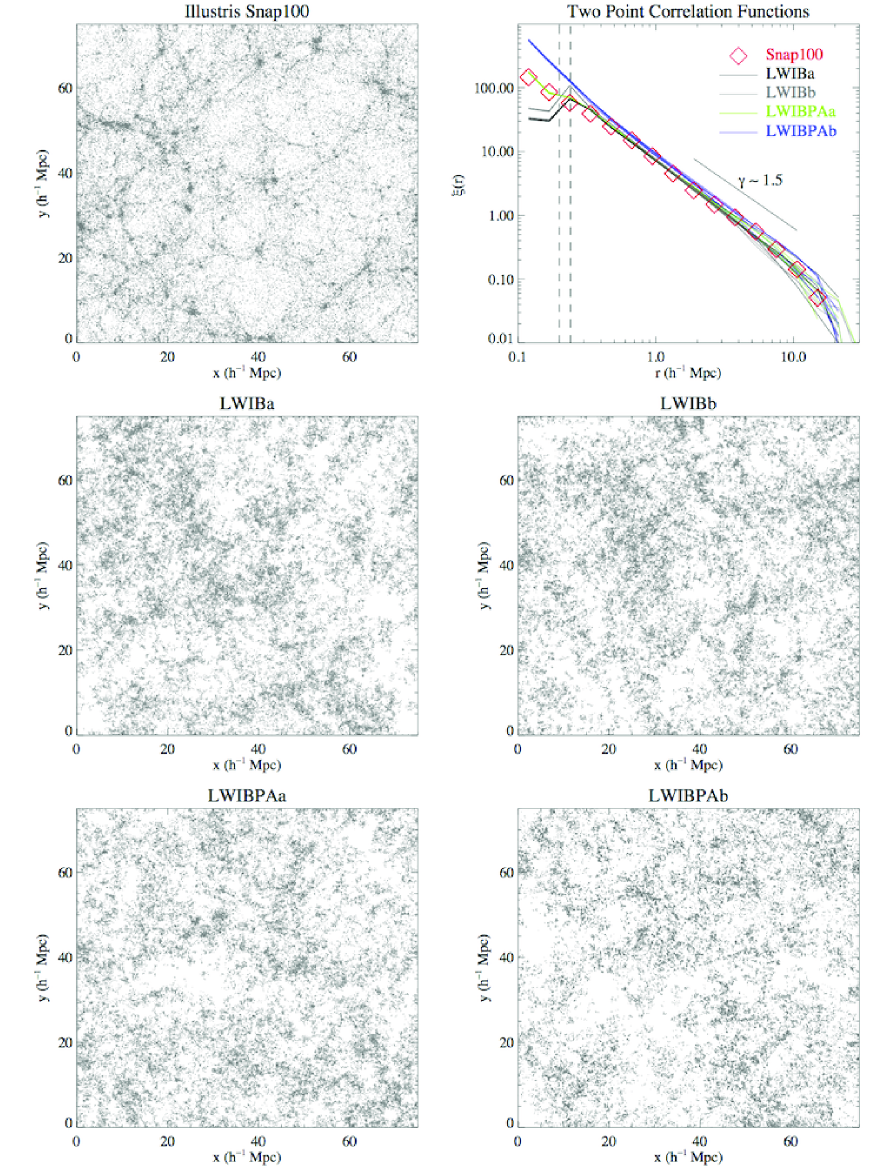
Figure 1.— The top-left panel shows the spatial distribution of the Illustris galaxy distribution at $z=0.58$ (“Snap100”) in comoving coordinates and the middle and bottom panels show Lévy walk galaxies with various parameters, summarized in Table 1. The top-right panel shows the two point correlation function for each sample. The dashed vertical lines represent the minimum step sizes of Lévy Walk models. We produce 100 realizations for each Lévy walk and, here, we present 5 measurements (hence, 5 lines for each) to illustrate ensemble variances. The major difference, even clear in visual inspection, between the cosmological simulation and Lévy fractals is the filamentary structure, which is absent in the Lévy fractal realizations.

IV. Results

IV.1. Missing Topologies in Two Point Correlation Function

In the previous section, we described our adopted simulation sets, Snap100, and Lévy walk recipes, and measured their two-point correlation functions, as summarized in Figure 1.

LWIBPAa yields a good match to the correlation function of Snap100, at least to the accuracy of practical clustering studies. LWIBa and LWIBPAb can be considered, respectively, as “lower” and “upper” bounds of correlation functions encompassing suppressed and enhanced small scale clustering. LWIBb is a model with slightly different parameters, $l_{0}=0.2$ and $\alpha=1.6$, from LWIBa, demonstrating that the clustering properties of LWIB models do not change abruptly by choosing parameters nearby. Hence, the four types of Lévy walk models illustrated in Figure 1 span a good range of possible Lévy fractals, comparable to Snap100.

The important point is that while the Lévy walk distributions reproduce the two-point correlation function of the galaxy distribution in the Illustris simulation, none of them mimic the actual spatial distribution of the Snap100 galaxies. In particular, the Lévy walks fail to reproduce the filamentary structure that is so characteristic of actual galaxy distributions. This implies that Lévy fractals are not appropriate for explaining the structure of the (simulated) Universe, and two-point statistics are highly degenerate. As noted in §II, this is because topological features are elusive in $n$-point statistics, while human eyes are more adapted to effectively recognize topologies of patterns and connectivities. Unlike what has been believed up to now, that such eye capturing features are hard to quantify, in the following sections we describe how such topologies can be measured using network science tools.

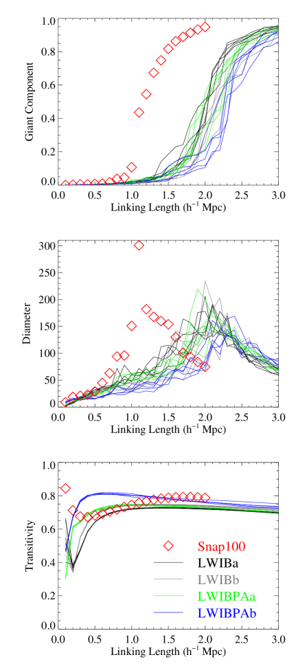
Figure 2.— The three network measurements, giant component fraction (top), diameter (middle), and transitivity (bottom) vs. linking length for the five models, the Illustris $z=0.58$ snapshot (“Snap100”) (red-open diamonds), LWIBa (black lines), LWIBb (grey lines), LWIBPAa (green lines), and LWIBPAb (blue lines). For each Lévy walk model, we plot 5 lines for 5 realizations like in Figure 1 to illustrate statistical variances. All the three network measurements show clear separations between Snap100 and Lévy fractals, implying that Lévy walk models fail to match the topological properties of Snap100. The galaxy distribution in the Illustris simulation is clearly not a Lévy fractal.

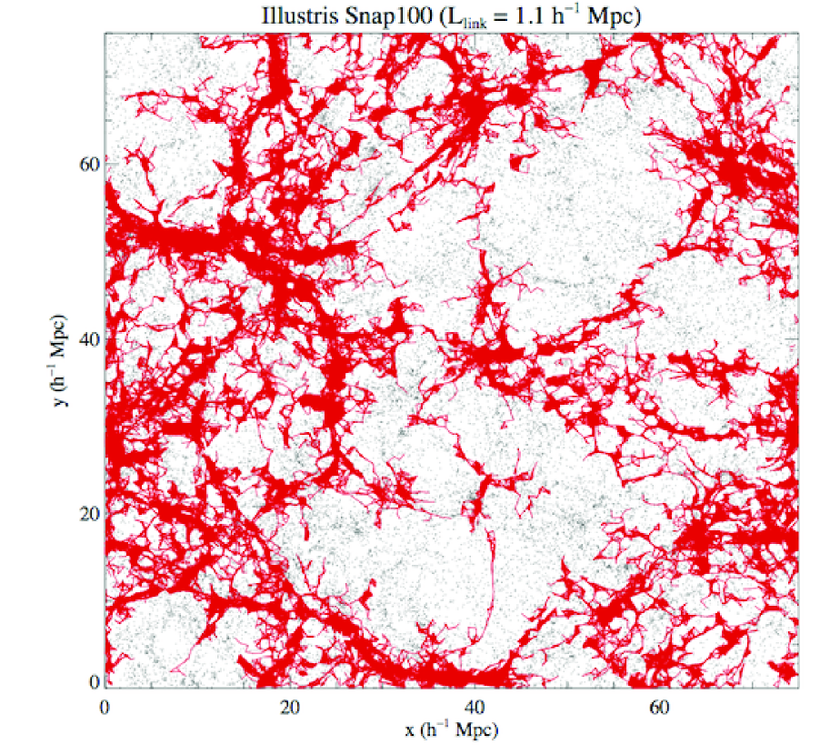
Figure 3.— The simulated galaxies of the Illustris $z=0.58$ snapshot (“Snap100”; grey dots) and edges connecting galaxies in the giant component (red line), visualizing the spatial network structure of the giant component. The linking length is $1.1~{}h^{-1}$Mpc, where the diameter is maximized. The texture of this Snap100 giant component can be described as “thin, diversifying, and filamentary”.

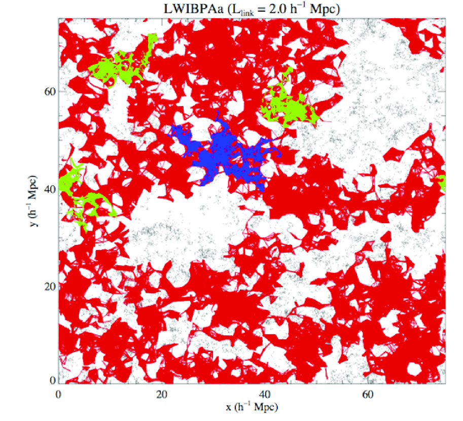
Figure 4.— The same as Figure  3 but for LWIBPAa. The linking length is $2.0~{}h^{-1}$Mpc, where the diameter for LWIBPAa is maximized. The texture of LWIBPAa’s giant component (red lines) can be described as “thick, clumpy, and modularized”. The blue lines show the edges of the giant component (hence, the largest component), and the green lines of the second, third, and fourth largest components, for the linking length $1.1~{}h^{-1}$Mpc, comparable to Figure  3. While the giant component of Snap100 shows a fully developed global structure at $1.1~{}h^{-1}$Mpc, the giant component (blue lines) and next largest components (green lines) of LWIBPAa are still localized due to the lack of topological bridges.

IV.2. Network Analysis: Quantifying Missing Topologies

A network is a data structure composed of “vertices” (or nodes) connected by “edges” (or links); also known as a graph in mathematics. In the 21st century, network science (or graph theory) has becomes one of the most critical tools in various fields, such as bioinformatics, computer science, physics, and sociology. In a previous work (HD15), we explored the use of network measures (betweenness, closeness and degree) to investigate the relationships between galaxy properties and topology. The results were promising, but limited by the use of photometric (rather than spectroscopic) redshifts to characterize the 3-dimensional galaxy distribution. Readers interested in networks are referred to Newman (2003), Dorogovtsev & Goltsev (2008), Barthélemy (2011), and HD15 for further information.

IV.2.1 Linking Length and Friends-of-friends Network

To build a network from a given galaxy population, we adopt the conventional friends-of-friends (FOF) recipe (e.g. Huchra & Geller 1984, More et al. 2011, HD15).

For a given linking length $l$, we define the adjacency matrix as,

$$A_{ij}=\left\{\begin{array}[]{ll}1&\textrm{ if }r_{ij}\leq l,\\ 0&\textrm{ otherwise, }\end{array}\right.$$ (4)

where $r_{ij}$ is the distance between the two vertices, $i$ and $j$. This binary matrix quantitatively represents the network connectivities of the FOF recipe. Many important network measures are derived from this matrix.

IV.2.2 Network Topologies : Diameter, Giant Component, and Transitivity

We measure three simple scalar quantities, diameter, giant component, and transitivity, from FOF networks for various linking lengths, using the open network library, igraph (Csardi & Nepusz 2006). Due to their simple definitions, these measures are computationally cheap and widely used in complex networks. The question is whether these network science tools can quantify the topological differences missed by two point statistics.

The Diameter is the largest path length of shortest-pathways from all pairs in a network. The path length is defined as the number of steps to reach from a certain vertex, $i$, to another, $j$. Hence, the pathways of minimum path length are the shortest pathways between the vertices, $i$ and $j$; generally, there can be multiple shortest pathways between a pair in an unweighted network. When a linking length is quite small to isolate all galaxies alone, the diameter is trivially 0. As the linking length is increased, the diameter grows to reach a certain maximum value. Since, for a very large linking length, all pairs are connected by a single direct edge (in the mathematical terms, forming a “complete graph”), the diameter asymptotically decreases to 1, after reaching the maximum value. Hence, this varying curve of Diameter vs. Linking Length is a quantified topology, depending on pathway structures.

The Giant component is the largest connected subgraph in a network. As in the case of diameter, giant components are trivial for the two extreme linking lengths. For a small linking length that isolates individual galaxies, the size of the giant component is 1. In the opposite case of a very large linking length forming a complete graph, the giant component size is equal to the total number of vertices (galaxies). Hence, the ratio of the size of the giant component to the total number of vertices is a fraction that increases from 0 to 1 monotonically with the linking length. The rate of growth of this ratio depends on topology; if a network has some topological structures to connect vertices more efficiently, the fraction of the giant component grows faster to reach 1 at a smaller linking length.

Transitivity can be described as a “triangle density” for a network. It is defined as:

$$C = \frac{\textrm{number of closed paths of length two}}{\textrm{number of paths of length two}},$$ (5)

where $C$ denotes the transitivity (Newman 2010). A path of length two means a “$\vee$” shaped connection; i.e. my friend-of-friend configuration in a social network. If my friend-of-friend is my direct friend, this path of length two forms a closed path of length two; i.e. a triangle “$\triangledown$”. Therefore, Equation 5 predicts a higher transitivity value if there are more triangles in a network. To some extent, transitivity can be considered as a minimal (and topological) version of the three point correlation function.

Figure 2 shows the three network quantities for our 5 samples, Snap100 (red-open diamonds), LWIBa (black lines), LWIBb (grey lines), LWIBPAa (green lines), and LWIBPAb (blue lines). As in Figure 1, for each Lévy walk model we plot 5 lines for 5 realizations to illustrate statistical variance. The three network quantities are uniquely determined for a given linking length. Namely, the three plots of diameter, giant component, and transitivity vs. linking length are self-consistently determined for a given spatial distribution like $n-$point statistics without any further parameter or assumption, except for their independent variable, linking length.

The top panel of Figure 2 shows the results for giant component fractions. Now we can quantitatively discern Snap100 (red-open diamonds) from LWIBPAa (green lines), though they have (practically) the same abundance and two-point correlation function, shown in Figure 1. All the other Lévy walk models also fail to match the growth curve of giant component fractions. When considering that LWIBa and LWIBPAb are, respectively, lower and upper bounds of the small-scale clustering for LWIBPAa (and Snap100), the failures of all Lévy walk models to match giant component fractions imply the fundamental difference in the pathway topology between Snap100 and Lévy fractals; Snap100 has more efficient pathways to connect all galaxies at a shorter linking length than Lévy fractals. Very likely, this is due to the filamentary structures in Snap100, lacking in Lévy fractals.

The middle panel of Figure 2 shows the diameters. We can again see clear separations of Snap100 from the Lévy walk models. Snap100 reaches the maximum diameter, 300, at the linking length, 1.1$h^{-1}$Mpc, while Lévy walk models reach the maximum diameters around 200 for linking lengths near 2.0$h^{-1}$Mpc. Even for 100 Lévy walk realizations, none of the Lévy walk models can match the diameter measurements of Snap100. Hence, both the size of the giant component and diameter are network measures that discriminate the Lévy walk topologies from the Illustris simulation, despite the data sets being constructed to have matching abundance and two-point correlation statistics.

The linking length for maximum diameter is related to the inflection point of the growth curve of giant component fractions; the rate of growth of the giant component decreases after reaching the maximum diameter. This transitioning feature occurs due to the “saturation” of connecting edges. At first (i.e., small linking length values), increasing the linking length results in adding new vertices and increasing the size of the connected network components. However, once the largest diameter is reached, increasing the linking length tends to form new pathways within the existing structure between more far-flung members and only slowly increases the overall size of the connected structure. Therefore, the diameter is maximized at this critical scale, transitioning from “growing phase” to “saturating phase”. The previous percolation studies are closely related to this maximum diameter scale, though they have not measured these specific diameters. If the system size is infinite, the diameter measurements transit from finite values to an infinity near this scale.

The bottom panel of Figure 2 shows transitivity results. Again, none of Lévy walk models mimic the transitivity curve of Snap100. We note that the statistical variances of transitivity measurements are much smaller than the other measurements as shown in Figure 2, since a single realization of the network is statistically large enough for counting triangles. Hence, the difference of transitivities between Snap100 and Lévy fractals also suggests that Snap100 is topologically very different from Lévy fractals.

An interesting feature is the difference of convexities between Snap100 (concave or “cup”) and Lévy fractals (convex or “hat”). The transitivities of Snap100 are high for small linking lengths, then decrease to a minimum transitivity at 0.4 $h^{-1}$Mpc as the linking length increases. After this, the transitivities slowly increase to 0.8. This transitivity trend of Snap100 is related to the transition between the one-halo term to the two-halo term in halo occupation clustering models (Berlind & Weinberg 2002). For small linking lengths, most triangles form in cluster environments reflecting halo substructures. Hence, these “intra-halo triangles” (i.e., triangles lying within one halo) dominate the transitivities for small linking lengths, and result in a decreasing trend from a very high transitivity. On the other hand, for sufficiently large linking lengths, “inter-halo triangles” (i.e., halo-halo-halo triangles) dominate over intra-halo triangles, simply because their configurations are more frequently found. Since a “$\vee$” shaped configuration becomes a triangle for a larger increased linking length, the transitivities for inter-halo scales are generally an increasing function. Therefore, this is potentially a very interesting point.

For Lévy walk models, the origins of triangles are different from Snap100. For scales smaller than the minimum Lévy walk step $l_{0}$ (0.2 $h^{-1}$Mpc and 0.24 $h^{-1}$Mpc in Table 1), the triangles originate from “random” encounters or our “proximity adjustment” recipe. For scales larger than the minimum Lévy walk steps, the fractal Lévy walks shape the rest of the triangles. Hence, discontinuities occur at these breaking scales in transitivity curves. The typical fractal transitivities increase to reach maximum values, and then asymptotically decrease to around 0.75. These convex (or “hat”) trends contrast to the concave (or “cup”) shape of Snap100.

Figure 3 shows the edges (red lines) connecting galaxies in the giant component of Snap100, visualizing the spatial network structure of the giant component. The linking length is 1.1$h^{-1}$Mpc, where the diameter is maximized. The texture of this Snap100 giant component can be described as “thin, diversifying, and filamentary”. Figure 4 shows the same as Figure 3 for LWIBPAa. The linking length is 2.0 $h^{-1}$Mpc, where the diameter for LWIBPAa is maximized. The texture of LWIBPAa’s giant component (red lines) can be described as “thick, clumpy, and modularized”. The blue lines show the edges of giant component for the linking length 1.1 $h^{-1}$Mpc, comparable to Figure  3. While the giant component of Snap100 shows a fully developed global structure at 1.1 $h^{-1}$Mpc, the giant component of LWIBPAa (blue lines) is still localized due to the lack of topological bridges. Overall, the structural and topological differences between Snap100 and Lévy fractals are well reflected in network structure.

Figure 5 presents two basic schemas to demonstrate which topological configuration can increase (or decrease) the transitivity. We note that variation of transitivity depends on very complex topological structures. The schemas are only two possible cases among many.

The top diagram of Figure 5 shows that the new vertex (asterisk) and edges (grey dashed lines) produce four additional “$\vee$” configurations, but none of them form a triangle; hence, transitivity decreases by this new vertex. This schema provides a possible illustration as to why Snap100 shows a decreasing transitivity trend at intra-halo scales. On the other hand, the bottom diagram of Figure 5 shows that the new vertex and edges form three additional triangles to increase the transitivity. Basically a linear chain of walks is less efficient in forming triangles than a gravitational pull to pack galaxies. This explains why Lévy walks show smaller transitivities at small scales than Snap100. However, such low transitivity values can be restored as the linking length increases as in the bottom diagram. Hence, the different behaviors of transitivity between Snap100 and Lévy fractals reflect the different topological bindings of galaxies (or walks); i.e., gravitationally packed solid ball vs. linearly tangled ball.

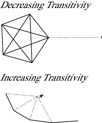
Figure 5.— Schemas demonstrating two possible cases to increase (top) and to decrease (bottom) transitivity values by adding a new vertex (asterisk) and its edges (dashed-grey lines). In the top diagram, the new dashed edge produces 4 additional “$\vee$” configurations, but none of them form triangles. On the other hand, in the bottom diagram, three triangles form by the new vertex and edges. Hence, the different convexities of transitivity curves for Snap100 and Lévy fractals reflect the intrinsic difference of topological structures.

V. Summary

In this paper we have used a network approach to compare two galaxy distributions with similar two-point correlation statistics but different topologies, one derived from a cosmological simulation and the other from a Lévy walk. The network measures are computed directly from the point distribution of the galaxies, unlike past measures that characterize a smoothed continuous version of the point distribution. We find that the simulated galaxies and Lévy walks are statistically different in diameter, giant component, and transitivity measurements, which shows that Lévy walks fail to mimic the topologies of the distribution of the simulated galaxies, though they successfully match the abundance and two point correlation function.

This implies that quantified topologies are important for testing cosmologies. While $n$-point statistics are undeniably useful diagnostics, their topological complementaries are necessary to properly test cosmologies and to prevent misinterpretation that could result from over-simplified false-positive models.

References

- (1) Adelberger, K. L., et al. 2005, ApJ, 619, 697
- (2) Albert, R., & Barabási A.-L., 2002, Reviews of Modern Physics, 74, 47
- (3) Alon, N., Yuster, R., & Zwick, U. 1997, Algorithmica, 17, 209
- (4) Aragón-Calvo M. A., Jones B. J. T., van de Weygaert R., van der Hulst J. M., 2007, A&A, 474, 315
- (5) Barkats, D. et al. 2014, ApJ, 783, 67
- (6) Barabási A.-L., 2009, Science, 325, 412
- (7) Barrow J. D., Bhavsar S. P., Sonoda D. H., 1985, MNRAS, 216, 17
- (8) Barthélemy, M. 2011, Physics Reports, 499, 1
- (9) Berlind, A. A., & Weinberg, D. H. 2002, ApJ, 575, 587
- (10) Bond N. A., Strauss M. A., Cen R., 2010, MNRAS, 409, 156
- (11) Csardi G., Nepusz T., 2006, InterJournal, Complex Systems, 1695 (http://igraph.org)
- (12) Cautun M., van de Weygaert R., Jones B. J. T., 2013, MNRAS, 429, 1286
- (13) Colberg J. M. 2007, MNRAS, 375, 337
- (14) Cormen, T. H., et al. 2009, Introduction to Algorithms, 3rd Edition, The MIT Press, Cambridge, Massachusetts
- (15) Davis, M. & Peebles, P. J. E. 1983, ApJ, 26, 465
- (16) Delubac, T., et al. 2015, A&A, 574, 59
- (17) Di Matteo, T. et al. 2005, Nature, 433, 604
- (18) Dorogovtsev, S. N., Goltsev, A. V., 2008, Rev. Mod. Phys., 80, 1275
- (19) Ducout, A. et al. 2013, MNRAS, 429, 2104
- (20) Euler L., 1741, Commentarii Acad. Sci. Petropolitanae, 8, 128
- (21) Eisenbrand, F., & Grandoni, F. 2004, Theoretical Computer Science, 326, 57
- (22) Eriksen, H. K. et al. 2004, ApJ, 612, 64
- (23) Genel, S., et al. 2014, MNRAS, 445, 175
- (24) Gil-Marin, H., et al. 2015, MNRAS, 451, 539
- (25) Gott J. R., Weinberg D. H., Melott A. L., 1987, ApJ, 319, 1
- (26) Hikage C. et al. 2008, MNRAS, 389, 1439
- (27) Hinshaw, G. et al. 2013, ApJS, 208, 19
- (28) Hong, S., & Dey, A. 2015, MNRAS, 450, 1999
- (29) Huchra, J. P. & Geller, M. J. 1982, ApJ, 257, 423
- (30) Keres, D., et al. 2012, MNRAS, 425, 2027
- (31) Kulkarni, G., et al. 2007, MNRAS, 378, 1196
- (32) Landy, S. D., & Szalay, A. S. 1993, ApJ, 412, 64
- (33) Levi, M. et al. 2013, arXiv:1308.0847
- (34) Lidz, A. et al. 2010, ApJ, 718, 199
- (35) Mandelbrot, B. 1975, C. R. Acad. Sci. (Paris) A280, 1551
- (36) Martínez V. J., Starck J.-L., Saar E., Donoho D. L., Reynolds S. C., de la Cruz P., Paredes S., 2005, ApJ, 634, 744
- (37) Mecke K. R., Buchert T., Wagner H., 1994, A&A, 288, 697
- (38) More, S., et al. 2011, ApJS, 195, 4
- (39) Nelson, D., et al. 2015, A&C, 13, 12
- (40) Nelson, D., et al. 2013, MNRAS, 429, 3353
- (41) Newman, M. E. J., 2003, SIAM Review, 45, 167
- (42) Newman, M. E. J., 2010, Networks: An Introduction. Oxford Univ. Press, Oxford
- (43) Park, C. et al. 2005, ApJ, 633, 11
- (44) Planck Collaboration, & Ade, P. A. R. et al. 2015, arXiv:1502.01592
- (45) Planck Collaboration, & Aghanim, N. et al. 2015, arXiv:1507.02704
- (46) Shandarin, S. F., 1983A, Pis’ma Astron. Zh. 9, 195 [Sov. Astron. Lett. 9, 104 (1983)] (A)
- (47) Shandarin, S. F., et al. 1983B, Usp. Fiz. Nauk 139, 83 [Sov. Pys. Usp. 26, 46 (1983)] (B)
- (48) Shandarin, S. F., & Zeldovich, Y. B., 1989, Reviews of Modern Physics, 61, 185
- (49) Sheth J. V., Sahni V., Shandarin S. F., Sathyaprakash B. S., 2003, MNRAS,343, 22
- (50) Sijacki, D., et al. 2012, MNRAS, 424, 2999
- (51) Sijacki, D., et al. 2012, MNRAS, 380, 877
- (52) Soneira, R. M., & Peebles, P. J. E. 1978, AJ, 83, 845
- (53) Sousbie T., Pichon C., Courtois H., Colombi S., Novikov D., 2008, ApJ, 672, L1
- (54) Springel, V. & Hernquist, L. 2003, MNRAS, 339, 289
- (55) Springel, V. et al. 2005, MNRAS, 361, 776
- (56) Springel, V. 2010, MNRAS, 401, 791
- (57) Tinker, J. 2007, MNRAS, 374, 477
- (58) Vogelsberger, M. 2014A, Nature, 509, 177 (A)
- (59) Vogelsberger, M., et al. 2014B, MNRAS, 444, 1518 (B)
- (60) Vogelsberger, M., et al. 2013, MNRAS, 436, 3031
- (61) Vogelsberger, M., et al. 2012, MNRAS, 425, 3024
- (62) Zhao, G, et al. 2015, arXiv:1510.08216
- (63) Zheng, Z., et al. 2005, ApJ, 633, 791
- (64) Zhu et al. 2015, ApJ, 800, 6