TTC: A high-performance Compiler for Tensor Transpositions

Abstract

We present TTC, an open-source parallel compiler for multidimensional tensor transpositions. In order to generate high-performance C++ code, TTC explores a number of optimizations, including software prefetching, blocking, loop-reordering, and explicit vectorization. To evaluate the performance of multidimensional transpositions across a range of possible use-cases, we also release a benchmark covering arbitrary transpositions of up to six dimensions. Performance results show that the routines generated by TTC achieve close to peak memory bandwidth on both the Intel Haswell and the AMD Steamroller architectures, and yield significant performance gains over modern compilers. By implementing a set of pruning heuristics, TTC allows users to limit the number of potential solutions; this option is especially useful when dealing with high-dimensional tensors, as the search space might become prohibitively large. Experiments indicate that when only 100 potential solutions are considered, the resulting performance is about 99% of that achieved with exhaustive search.

Author’s address: P. Springer (springer@aices.rwth-aachen.de) and P. Bientinesi (pauldj@aices.rwth-aachen.de), AICES, RWTH Aachen University, Schinkelstr. 2, 52062 Aachen, Germany. acmlicensed http://dx.doi.org/10.1145/0000000.0000000 0098-3500

1 Introduction

Tensors appear in a wide range of applications, including electronic structure theory [Bartlett and Musiał (2007)], multiresolution analysis [Harrison et al. (2015)], quantum many-body theory [Pfeifer et al. (2014)], quantum computing simulation [Markov and Shi (2008)], machine learning [Chetlur et al. (2014), Abadi et al. (2015), Vasilache et al. (2014)], and data analysis [Kolda and Bader (2009)]. While a range of software tools exist for computations involving one- and two-dimensional arrays, i.e. vectors and matrices, the availability of high-performance software tools for tensors is much more limited. In part, this is due to the combinatorial explosion of different operations that need to be supported: There are only four ways to multiply two matrices, but $\binom{m}{k}\binom{n}{k}$ ways to contract an $m$- and an $n$-dimensional tensor over $k$ indices. Furthermore, the different dimensions and data layouts that are relevant to applications are much larger in the case of tensors, and these issues lead to memory access patterns that are particularly difficult to execute efficiently on modern computing platforms.

Efficient computation of tensor operations, particularly contractions, exposes a tension between generality and mathematical expression on one hand, and performance and software reuse on the other. If one implements tensor contractions in a naive way—using perfectly-nested loops—the connection with the mathematical formulae is obvious, but the performance will be suboptimal in all nontrivial cases. High performance can be obtained by using the Basic Linear Algebra Subprograms (BLAS) [Dongarra et al. (1990)], but mapping from tensors to matrices efficiently is nontrivial [Di Napoli et al. (2014), Li et al. (2015)] and optimal strategies are unlikely to be performance portable, due to the ways that multidimensional array striding taxes the memory hierarchy of modern microprocessors.

A well-known approach for optimizing tensor computations is to use the level-3 BLAS for contracting matrices at high efficiency, and to always permute tensor objects into a compatible matrix format. This approach has been used successfully in the NWChem Tensor Contraction Engine module [Hirata (2003), Kowalski et al. (2011)], the Cyclops Tensor Framework [Solomonik et al. (2014)], and numerous other coupled-cluster codes dating back more than 25 years [Gauss et al. (1991)]. The critical issue for this approach is the existence of a high-performance tensor permutation, or tensor transpositions.

While tensor contractions appear in a range of scientific domains (e.g., climate simulation [Drake et al. (1995)] and multidimensional Fourier transforms [Frigo and Johnson (2005), Pekurovsky (2012)]), they are perhaps of greatest importance in quantum chemistry [Baumgartner et al. (2005), Hirata (2003)], where the most expensive widely used methods—coupled-cluster methods—consist almost entirely of contractions which deal with 4-, 6-, and even 8-dimensional tensors. Such computations consume millions of processor-hours of supercomputing time at facilities around the world, so any improvement in their performance is of significant value.

To this end, we developed Tensor Transpose Compiler (TTC), an open source code generator for high-performance multidimensional transpositions that also supports multithreading and vectorization. Together with TTC, we provide a transpose benchmark that can be used to compare different algorithms and implementations on a range of multidimensional transpositions.

Let $A_{i_{1},i_{2},...,i_{N}}$ be an $N$-dimensional tensor, and let $\Pi(i_{1},i_{2},...,i_{N})$ denote an arbitrary permutation of the indices $i_{1},i_{2},...,i_{N}$. The transposition of $A$ into $B_{\Pi(i_{1},i_{2},...,i_{N})}$ is expressed as $B_{\Pi(i_{1},i_{2},...,i_{N})}\leftarrow\alpha\times A_{i_{1},i_{2},...,i_{N}}$. To make TTC flexible and applicable to a wide range of applications, we designed it to support the class of transpositions

$$B_{\Pi(i_{1},i_{2},...,i_{N})}\leftarrow\alpha\times A_{i_{1},i_{2},...,i_{N}}+\beta\times B_{\Pi(i_{1},i_{2},...,i_{N})},$$ (1)

where $\alpha$ and $\beta\in\mathbb{R}$; that is, the output tensor $B$ can be updated (as opposed to overwritten), and both $A$ and $B$ can be scaled. As an example, let $A_{i_{1},i_{2}}$ be a two-dimensional tensor, $\Pi(i_{1},i_{2})=(i_{2},i_{1})$, and $\alpha=1,\beta=0$; then Eqn. 1 reduces to an ordinary out-of-place 2D matrix transposition of the form $B_{i_{2},i_{1}}\leftarrow A_{i_{1},i_{2}}$.

Throughout this article, we adopt a Fortran storage scheme, that is, the tensors are assumed to be stored following the indices from left to right (i.e., the leftmost index has stride 1). Additionally, we use the notation $\pi(i_{a})=i_{b}$ to denote that the $a$^th index of the input operand will become the $b$^th index of the output operand.

For each input transposition, TCC explores a number of optimizations (e.g., blocking, vectorization, parallelization, prefetching, loop-reordering, non-temporal stores), each of which exposes one or more parameters; to achieve high-performance, these parameters have be tuned for the specific hardware on which the transposition will be executed. Since the effects of such parameters are non-independent, the optimal configuration is a point (or a region) of an often large parameter space; indeed, as the size of the space grows as $N!$, an exhaustive search is feasible only for tensors of low dimensionality. In general, it is widely believed that the parameter space is too complex to design a perfect transpose from first principles [McCalpin and Smotherman (1995), Lu et al. (2006)]. For all these reasons, whenever an exhaustive search is not applicable, TTC’s generation relies on heuristics.

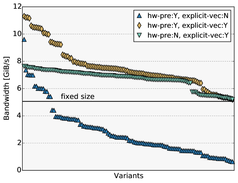
(a) $\Pi(i_{1},i_{2},i_{3},i_{4},i_{5})=(i_{2},i_{5},i_{3},i_{1},i_{4})$

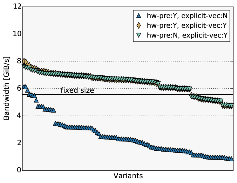
(b) $\Pi(i_{1},i_{2},i_{3},i_{4},i_{5})=(i_{5},i_{3},i_{1},i_{4},i_{2})$

Figure 1: Single-threaded bandwidth for all the 120 possible loop orders of two different 5D transpositions. explicit-vec and hw-pre respectively denote whether explicit vectorization and hardware prefetching are enabled (Y) or disabled (N).

In Fig. 1, we use two exemplary 5D transpositions (involving tensors of equal volume), as compelling evidence in favor of a search-based approach. The figures show the bandwidth attained by each of the possible $5!=120$ loop orders—sorted in descending order, from left to right—with and without hardware prefetching (hw-pre:N, hw-pre:Y), and with and without explicit vectorization (explicit-vec:Y, explicit-vec:N). The compiler-vectorized code consists of perfectly nested loops including #pragma ivdep, to assist the compiler. The horizontal line labeled “fixed size” denotes the performance of the compiler-vectorized versions (with hardware prefetching enabled), where the size of the tensor was known at compile time; this enabled the compiler to reorder the loops.

Several observations can be made. (1) Despite the fact that the two transpositions move exactly the same amount of data, the resulting top bandwidth is clearly different. (2) The difference between the leftmost and the rightmost datapoints—of any color—provides clear evidence that the loop order has a huge impact on performance: $9.2\times$ and $4.3\times$ in Fig. 1(a) and Fig. 1(b), respectively. This is in line with the findings of Jeff Hammond [Hammond (2009)], who pointed out that the best loop order for a multidimensional transpose can have a huge impact on performance. (3) By comparing the leftmost data point of the beige () and blue lines (), one concludes that the explicit vectorization improves the performance over the fastest compiler-vectorized version by at least $20\%$. (4) Since the cyan () lines in Fig. 1(a) and 1(b) are practically the same, one can conclude that the difference in performance between the two transpositions is due to hardware prefetching. (5) The difference between the blue line () and the horizontal black line in Fig. 1(a) indicates that when it is possible for the compiler to reorder the loops, the code generated is much better than most loop orders, but still about 40% away from the best one; similarly for Fig. 1(b), the compiler fails to identify the best loop order.

While observation (5) suggests that modern compilers struggle to find the best loop order at compile time, an even bigger incentive to adopt a search-based approach is provided by observation (4), since detailed information about the mechanism of hardware prefetchers is not well-documented. Moreover, the implementations of hardware prefetchers can vary between architectures and manufactures. Hence, designing a generic analytical model for different architectures seems infeasible at this point.

The contributions of this paper can be summarized as follows.

• We introduce TTC, a high-performance transpose generator that supports single, double, single-complex, double-complex and mixed precision data types, generates multithreaded C++ code with explicit vectorization for AVX-enabled processors, and exploits spatial locality.

• We also introduce a comprehensive multidimensional transpose benchmark, to provide the means of comparing different implementations. By means of this benchmark, we perform a thorough performance comparison on two architectures.

• We analyze both the effects of four different optimizations in isolation, and quantify the impact of a dramatic reduction of the search space.

The remainder of the paper is structured as follows. Section 2 summarizes the related work on tensor transpositions. In Section 3 we introduce TTC with a special focus on its optimizations. In Section 4 we present a thorough performance analysis of TTC’s generated implementations—showing both the attained peak bandwidth as well as the speedups over a realistic baseline implementation. Finally, Section 5 concludes our findings and outlines future work.

2 Related Work

McCalpin et al. [McCalpin and Smotherman (1995)] realized that search is necessary for high-performance 2D transpositions as early as 1995. Their code-generator explored the optimization space in an exhaustive fashion.

Mateescu et al. [Mateescu et al. (2012)] developed a cache model for IBM’s Power7 processor. Their optimizations include blocking, prefetching and data alignment to avoid conflict-misses. They also illustrate the effect of large TLB page sizes on performance.

Lu et al. [Lu et al. (2006)] developed a code-generator for 2D transpositions using both an analytical model and search. They carried out an extensive work covering vectorization, blocking for both L1 cache and TLB, while parallelization was not explored.

Andre Vladimirov’s [Vladimirov (2013)] presented his research on in-place, square transpositions on Intel Xeon and Intel Xeon Phi processors.

Chatterjee et al. [Chatterjee and Sen (2000)] investigated the effect of cache and TLB misses on performance for square, in-place, 2D transpositions. Among other things, they concluded that “the limited number of TLB entries can easily lead to thrashing” and that “hierarchical non-linear layouts are inherently superior to the standard canonical layouts”.

While there has been a lot of research targeted on 2D transpositions [McCalpin and Smotherman (1995), Mateescu et al. (2012), Goldbogen (1981), Vladimirov (2013), Chatterjee and Sen (2000), Lu et al. (2006)] and 3D transpositions [Jodra et al. (2015), Ding (2001), van Heel (1991)], higher dimensional transpositions have not yet experienced the same level of attention.

Ding et al. [Ding (2001), He and Ding (2002)] present an algorithm dedicated to multidimensional in-place transpositions. Their approach is optimal with respect to the number of bytes moved. However, their results suggest that this approach does not yield good performance if the position of the stride-1 index changes (i.e., $\pi(i_{1})\neq i_{1}$).

The work of Wei et al. [Wei and Mellor-Crummey (2014)] is probably the most complete study of multidimensional transpositions so far. Their code-generator, which “uses exhaustive global search”, explores blocking, in-cache buffers to avoid conflict misses [Gatlin and Carter (1999)], loop unrolling, software prefetching and vectorization. The generated code achieves a significant percentage of the system’s memcpy bandwidth on an Intel Xeon and an IBM Power7 node for cache-aligned transpositions. However, a parallelization approach is not described, and different loop orders are not considered.

Lyakh et al. [Lyakh (2015)] designed a generic multidimensional transpose algorithm and evaluated it across different architectures (e.g., Intel Xeon, Intel Xeon Phi, AMD and NVIDIA K20X). In contrast to our approach, theirs does not rely on search. Their results suggest that on both the Xeon Phi as well as the NVIDIA architectures, there still is a significant performance gap between their transposition algorithm and a direct copy.

3 Tensor Transpose Compiler

TTC is a domain-specific compiler for tensor transpositions of arbitrary dimension. It is written in Python and generates high-performance C++ code. For a given permutation and tensor-size, TTC explores a search space of possible implementations. These implementations differ in some properties which have direct effects on performance e.g., loop order, prefetch distance, blocking; each of such properties will be discussed in the following sections. Henceforth, we use the term ‘candidate’ for all these implementations; similarly, we use the term ‘solution’ to denote the fastest (i.e., best performing) candidate.

To reduce the compilation time, TTC allows the user to limit the number of candidates to explore; by default, TTC explores up to 200 candidates. Unless the user specifically wants to explore the entire search space exhaustively, TTC applies heuristics to prune the search space and to identify promising candidates that are expected to yield high performance. A good heuristic should be generic enough to be applicable on different architectures, and it should prune the search space to a degree so that the remaining implementations can be evaluated exhaustively. Once the search space has been pruned, TTC generates the C++ routines for all the remaining candidates, which are compiled and timed.

Argument	Description
--perm=<index1>,<index2>,$\dots$	permutation∗
--size=<size1>,<size2>,$\dots$	size of each index∗
--dataType=<s,d,c,z,sd,ds,cz,zc>	data type of $A$ and $B$ (default: s)
--alpha=<value>	alpha (default: 1.0)
--beta=<value>	beta (default: 0.0)
--lda=<size1>,<size2>,$\dots$	leading dimension of each index of $A$
--ldb=<size1>,<size2>,$\dots$	leading dimension of each index of $B$
--prefetchDistances=<value>,$\dots$	allowed prefetch distances
--no-streaming-stores	disable non-temporal stores (default: off)
--blockings=<H$\times$W>,$\dots$	block sizes to be explored
--maxImplementations=<value>	max #implementations (default: 200)

Table 1: TTC’s command-line arguments. Required arguments are marked with a ^∗.

The minimum required input to the compiler is the actual permutation and the size of each index; several additional arguments to pass extra information and to guide the code generation process can be supplied by command-line arguments; a subset of the input arguments is listed in Table 1. For instance, by using the --lda and --ldb arguments, it is possible to transpose tensors that are a portion of larger tensors. This feature is particularly interesting because it enables TTC to generate efficient packing routines of scattered data elements into contiguous buffers; such routines are frequently used in dense linear algebra algorithms such as a matrix-matrix multiplication [Low et al. (2015)]. Moreover, TTC supports single-, double-, single-complex- and double-complex data types for both the input $A$ and the output $B$—via --dataType. TTC is also able to generate mixed-precision transpositions—where $A$ and $B$ are of different data type (e.g., --dataType=sd denotes that $A$ uses single-precision while $B$ uses double-precision). This feature is again especially interesting in the context of linear algebra libraries since it allows to implement mixed-precision routines effortlessly. Furthermore, the user can guide the search by choosing certain blockings, prefetch distances or loop orders—and thereby reduce the search space. With the argument --maxImplementations, the user influences the compile time by imposing a maximum size to the search space; in the extreme case in which this flag is set to one, the solution is returned without performing any search. On the other hand, setting --maxImplementations=-1 effectively disables the heuristics and instructs TTC to explore the search space exhaustively.

A flowchart outlining the stages (1) - (9) of TTC is shown in Fig. 2. (1) To reduce complexity, TTC starts off by merging indices, whenever possible, in the input and output tensor. For instance, given the permutation $\Pi(i_{1},i_{2},i_{3})=(i_{2},i_{3},i_{1})$, the indices $i_{2}$ and $i_{3}$ are merged into a new ‘super index’ $\tilde{i_{2}}:=(i_{2},i_{3})$ of the same size as the combined indices (i.e., size($\tilde{i_{2}}$) $=$ size($i_{2}$)$\times$size($i_{3}$)); as a consequence, the permutation becomes $\Pi(i_{1},\tilde{i_{2}})=(\tilde{i_{2}},i_{1})$. Next, TTC queries a local SQL database of known/previous solutions, to check whether a solution for the input transposition already exists; if so, no generation takes place, and the previous solution is returned. Otherwise, the code-generation proceeds as follows: (2) one of the possible blockings is chosen, (3) a loop order is selected, and (4) other optimizations (e.g., software prefetching, streaming-stores) are set. The combination of the chosen blocking, the loop order and the optimizations uniquely identify a candidate. After these steps, (5) an estimated cost for the current candidate is calculated. This cost is used to determine whether the current candidate should be added to a queue of candidates or if it should be neglected. The aforementioned input argument --maxImplementations determines the capacity of this queue.

The loop starting and ending at (2) is repeated, if different combinations of blockings, loop orders and optimizations are still possible. Once all candidates have been generated, they are (7) compiled by an external C++ compiler, and (8) timed. Finally, (9) the best candidate (i.e., the solution) is selected and stored to a .cpp/h file and its timing information as well as its properties (e.g., blocking, loop order) are saved in the SQL database for future references.

Figure 2: Schematic overview of our tensor transpose compiler TTC; vectorization and parallelization are always enabled.

For each and every transposition, TTC explores the following tuning opportunities:

• Explicit vectorization (Section 3.1)

• Blocking (Section 3.2)

• Loop-reordering (Section 3.3)

• Software prefetching (Section 3.4)

• Parallelization (Section 3.5)

• Non-temporal stores, if applicable

The following sections discuss these optimizations in greater detail. For the remainder of this article, let $w$ denote the vector-width, in elements, for any given precision and architecture (e.g., $w=8$ for single-precision calculations on an AVX-enabled architecture).

3.1 Vectorization

With respect to vectorization, we distinguish two different cases: the stride-1 index (i.e., the leftmost index) of the input and output tensors is constant (see Fig. 3(a)) or not (see Fig. 3(b)). To achieve optimal performance, these cases require significantly different implementations.

(a) Case 1: $\pi(i_{1})=i_{1}$

(b) Case 2: $\pi(i_{1})\neq i_{1}$

Figure 3: Two exemplary 3D transpositions.

3.1.1 Case 1: $\pi(i_{1})=i_{1}$

When the stride-1 index does not change, vectorization is straightforward. In this case, the transposition moves a contiguous chunk of memory (i.e., the first column) of the input/output tensor at once as opposed to a single element. Hence, the operation is essentially a series of nested loops around a memcopy of the size of the first column. In terms of the memory access pattern, this scenario is especially favorable, because of the available spatial data locality. Since the vectorization in this case does not require any in-register transpositions and merely boils down to a couple of vectorized loads and stores, we leave the vectorization to the compiler, which in this specific scenario is expected to yield good performance.

3.1.2 Case 2: $\pi(i_{1})\neq i_{1}$

In order to take full advantage of the SIMD capabilities of modern processors, this second case requires a more sophisticated approach. Without loss of generality, let us assume that the index $i_{b}$, with $i_{b}\neq i_{1}$, will become the stride-1 index in $B$ (e.g., $i_{b}=i_{3}$ in Fig. 3(b)). Accesses to $B$ are contiguous in memory for successive values of $i_{b}$, while accesses to $A$ are contiguous for successive values of $i_{1}$. Full vectorization is achieved by unrolling the $i_{1}$ and $i_{b}$ loops by multiples of $w$ elements, giving raise to an $w\times w$ transpose. Henceforth, we refer to such a $w\times w$ tile as a micro-tile. The transposition of a micro-tile is fully vectorized by using an in-register transposition. Using this scheme, an arbitrarily dimensional out-of-place tensor transposition is reduced to a series of independent two-dimensional $w\times w$ transpositions, each of which accesses $w$ many $w$-wide consecutive elements of both $A$ and $B$.

3.2 Blocking

In addition to the $w\times w$ micro-tiles, we introduce a second level of blocking to further increase locality. The idea is to combine multiple micro-tiles into a so-called macro-tile of size $b_{A}\times b_{B}$, where $b_{A}$ and $b_{B}$ correspond to the blocking in the stride-1 index of $A$ and $B$, respectively. This approach is illustrated in Fig. 4.

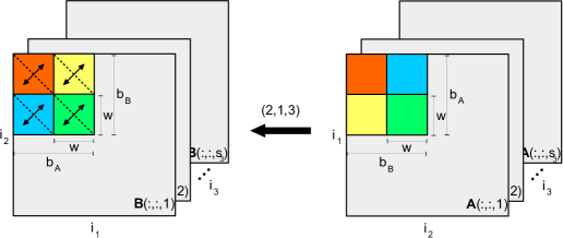
Figure 4: Overview of the blocking mechanism for the permutation $\Pi(i_{1},i_{2},i_{3})=(i_{2},i_{1},i_{3})$, with $b_{A}=b_{B}=2w$.

By default, TTC explores the search space of all macro-tiles of size $b_{A}\times b_{B}$ with $b_{A},b_{B}\in\{w,2w,3w,4w\}$. The flexibility of supporting multiple sizes of macro-tiles has several desirable advantages: first, it enables TTC to adapt to different memory systems, which might favor contiguous writes (e.g., $16\times 32$) over contiguous reads (e.g., $32\times 16$) and vice versa; second, it implicitly exploits architectural features such as adjacent cacheline prefetching, and cacheline-size (e.g., $16$ elements for single precision for modern x86 CPUs); finally, it reduces false-sharing of cache lines between different threads in a parallel setting.

If desired by the user, TTC can effectively prune the search space and only evaluate the performance of a subset of the available tiles. We designed a heuristic which ranks the blockings for a given transposition and size. Specifically, the blocking is chosen such that (1) $b_{A}$ and $b_{B}$ are both multiples of the cacheline-size (in elements), and that (2) the remainder $r^{i}=S^{i}_{1}\text{(mod) }b_{i},i\in\{A,B\}$, with $S^{i}_{1}$ being the size of the stride-1 index of tensor $i\in\{A,B\}$, is minimized. The quality of this heuristic is demonstrated in Section 4.4.

3.3 Loop order

As Fig. 1 already suggested, the choice of the proper loop order has a significant influence on performance. Since the number of available orderings for a tensor with $d$ dimensions is $d!$, determining the best loop order is by exhaustive search is expensive even for modest values of $d$.

Our heuristic to choose the loop order is designed to increase data locality in both $A$ and $B$. This strategy fulfills multiple purposes: (1) it reduces cache- and TLB-misses, and (2) it reduces the stride within the innermost loop. The latter is especially important because large strides can prevent modern hardware prefetchers from learning the memory access patterns. For instance, the maximal stride supported by hardware prefetchers of Intel Sandy Bridge CPUs is limited to $2\text{\,}\mathrm{KiB}$ [Intel Corporation (2015)]. Other aspects of the hardware implementation affect the cost of different loop orders; for example, the write-through cache policy of the IBM Blue Gene/Q architecture makes it extremely important to exploit write locality, since writing to a cache line evicts it from cache [Finkel (2015)]. The reader interested in further details on this heuristic is referred to the available source-code at www.github.com/HPAC/TTC.

3.4 Software Prefetching

Software prefetching is only enabled for the case of $\pi(i_{1})\neq i_{1}$; indeed, the memory access pattern for $\pi(i_{1})=i_{1}$ is so regular that it should be easily caught by the hardware prefetcher.

We designed the software prefetching to operate on micro-tiles; hence, a given prefetch distance $d$ has the same meaning irrespective of the chosen macro-blocking. The prefetching mechanism is depicted in Fig. 5. TTC always prefetches entire $w\times w$ micro-tiles. Before transposing the current micro-tile $j$, TTC prefetches the micro-tile which is at distance $d$ ahead of the current tile. This is illustrated by the colors in Fig. 5, where the macro-tile contains $n=4$ micro-tiles: before processing the orange $w\times w$ block of the current macro-tile $A_{i}$, TTC already prefetches the orange micro-tile of the corresponding macro-tile $A_{p}$, with $p=i+\lfloor(j+d)/n\rfloor$ (i.e., $A_{i+1}$ in Fig. 5).

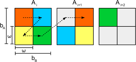
Figure 5: Overview of the software prefetching mechanism for a distance $d=5$. Arrows denote the order in which the micro-tiles are being processed.

3.5 Parallelization

⬇

1//variable declaration

2...

3

4//main loops

5#pragma omp parallel

6#pragma omp for collapse(3) schedule(static)

7 for(int i3 = 0; i3 < size2 - 15; i3+= 16)

8 for(int i1 = 0; i1 < size0 - 31; i1+= 32)

9 for(int i2 = 0; i2 < size1; i2+= 1)

10 transpose32x16(&A[i1 + i2*lda1 + i3*lda2], lda2,

11 &B[i1*ldb2 + i2*ldb1 + i3], ldb2, alpha, beta);

12//remainder loops

13...

Listing 1: Parallel code generated by TTC for the permutation ($i_{3},i_{2},i_{1}$).

Listing 1 contains the generated parallel code for a given tensor transposition with software prefetching disabled. The collapse clause increases the available parallelism and improves load balancing among the threads. Each thread has to process roughly the same amount of $b_{A}\times b_{B}$ tiles.

A detailed description of the parallelization of the prefetching algorithm is beyond the scope of this paper. However, the overall idea of prefetching the blocks remains identical to the scalar version (see previous section). The only difference is that each thread has to keep track of the tiles it will access in the near future in a local data structure; for this task, we use a queue of tiles. The interested reader is again referred to the source-code for further details.

4 Performance Evaluation

We evaluate the performance of TTC on two different systems, Intel and AMD. The Intel system consists of two Intel Xeon E5-2680 v3 CPUs (with 12 cores each) based on the Haswell microarchitecture. For all measurements, ECC is enabled, and both Intel Speedstep and Intel TurboBoost are disabled. The compiler of choice is the Intel icpc 15.0.4 with flags -O3 -openmp -xhost. Unless otherwise mentioned, this is the default configuration and system for the experiments. The AMD system consists of a single AMD A10-7850K APU with 4 cores based on the steamroller microarchitecture. The compiler for this system is gcc 5.3 with flags -O3 -fopenmp -march=native. All measurements are based on 24 threads and 4 threads for the Intel and AMD system, respectively (i.e., one thread per physical core).

Experimental results suggest that optimal performance is attained with one thread per physical core. We also experimented with thread affinity on both systems.

The reported bandwidth $\text{BW}(x)$ for solution $x$ is computed as

$$\text{BW}(x)=\frac{3\times S}{2^{30}\times\text{Time}(x)}\text{ }$\text{\,}\mathrm{GiB}$/s,$$ (2)

where $S$ is the size in bytes of the tensor; the prefactor $3$ is due to the fact that since in all our measurements $B$ is updated (i.e., $\beta\neq 0$, see Eqn. 1), one has to account for reading $B$ as well.

The reported memory bandwidth by the STREAM benchmark [McCalpin (1995)] for the Intel (AMD) system is 105.6 (12.2), 105.9 (12.2), 111.6 (13.1) and 112.2 (13.0) GiB/s for the copy ($\mathbf{b}\leftarrow\mathbf{a}$), scale ($\mathbf{b}\leftarrow\alpha\mathbf{a}$), add ($\mathbf{c}\leftarrow\mathbf{a}+\mathbf{b}$) and triad ($\mathbf{c}\leftarrow\alpha\mathbf{a}+\mathbf{b}$) test-cases, respectively.

4.1 Transposition Benchmark

To evaluate the performance of multidimensional transpositions across a range of possible use-cases, we designed a synthetic benchmark. The benchmark comprises 19 different transpositions, chosen so that no indices can be merged. For each tensor dimension (2D–6D), we included the inverse permutation (e.g., $B_{i_{3},i_{2},i_{1}}\leftarrow A_{i_{1},i_{2},i_{3}}$, $B_{i_{4},i_{3},i_{2},i_{1}}\leftarrow A_{i_{1},i_{2},i_{3},i_{4}}$, …), and exactly one permutation for which the stride-1 index does not change. These two scenarios typically cover both ends of the spectrum, yielding the worst and the best performance, respectively.

In the benchmark, each transposition is evaluated in three different configurations—for a total of 57 test cases: one where all indices are of roughly the same size, and two where the tensors have a ratio of $6$ between the largest and smallest index. The desired volume of the tensors across all dimensions are roughly the same and can be chosen by the user; in our experiments, we fixed it to $200\text{\,}\mathrm{MiB}$, which is bigger than any L3 cache in use today.

The benchmark is publicly available at www.github.com/HPAC/TTC/benchmark.

4.2 TTC-generated code

We now present the performance of the fastest implementations—generated by TTC—for all transpositions in the benchmark. Furthermore, we analyze the influence of the individual optimizations (blocking, loop-reordering, software prefetching, and explicit vectorization) on the performance.

Fig. 6 illustrates the attained bandwidth and speedup across the benchmark for the Intel and AMD systems. The speedups are measured over a reference routine consisting of $N$ perfectly nested loops annotated with both #pragma omp parallel for collapse($N-1$) on the outermost loop, and #pragma omp simd on the innermost loop. Moreover, the loop order for the reference version is chosen such that the output tensor $B$ is accessed in a perfectly linear fashion; this loop order reduces false sharing of cache lines between the threads. With this setup, the compiler is assisted as much as possible to yield a competitive routine.

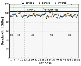
(a) Intel: Bandwidth.

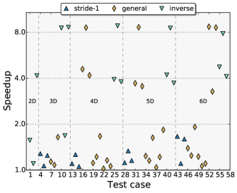
(b) Intel: Speedup.

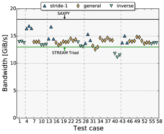
(c) AMD: Bandwidth.

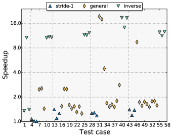
(d) AMD: Speedup.

Figure 6: TTC. Bandwidth and speedup of TTC’s fastest solution across the benchmark for the Intel and AMD system. The vertical lines identify the dimensionality of the tensors.

Figs. 6(a) and 6(c) show the attained bandwidth of the TTC-generated solutions across the benchmark for the Intel and AMD system, respectively. The transpositions are classified in three categories: stride-1 (), inverse (), and general (), respectively denoting those permutations in which the first index does not change, the inverse permutations, and those transpositions which do not fall into either of the previous two categories. In addition to the bandwidth, these figures also report the STREAM-triad bandwidth (solid green line), as well as the bandwidth of a SAXPY (i.e., single-precision vector-vector addition of the form $\mathbf{y}\leftarrow\alpha\mathbf{x}+\mathbf{y}$, $\alpha\in\mathbb{R},\mathbf{x,y}\in\mathbb{R}^{n}$, see solid black line). The figures illustrate that TTC achieves a significant fraction of the SAXPY-bandwidth on both architectures (the average across the entire benchmark is $91.68\%$ and $78.30\%$ for the Intel and AMD systems, respectively). With the exception of some performance-outliers on the AMD system, the performance of TTC is stable across the entire benchmark.

It is interesting to note that on the AMD system, TTC attains much higher bandwidth than the STREAM-triad benchmark. This phenomenon is due the fact that the STREAM benchmark does not account for the write-allocate traffic .

In terms of speedups over the reference implementation, TTC achieves considerable results on both systems (see Fig. 6(b) and 6(d)). When looking closely at the plots, it becomes apparent that the inverse permutations benefit the most from TTC, attaining speedups of up to $8.84\times$ and $18.15\times$ on the Intel and AMD system, respectively. While the speedups for the stride-1 transpositions are much smaller, they can still be as high as $1.66\times$. For general transpositions, the speedups range from $1.02\times$ to $8.71\times$, and from $1.28\times$ to $19.44\times$, for the Intel and AMD system, respectively.

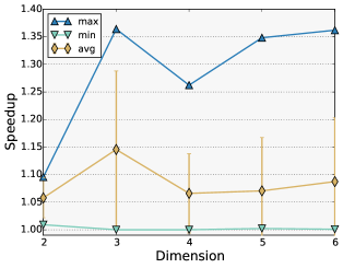
(a) Blocking

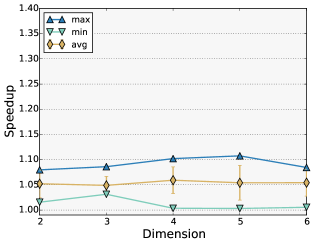
(b) Software prefetching

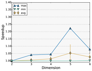
(c) Loop-reordering

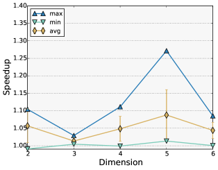
(d) Explicit vectorization

Figure 7: Breakdown of the speedups for the Intel system.

To gain insights on where the performance gains come from, in Fig. 7 we report the speedup due to each of TTC’s optimizations separately. For each test-case from the benchmark, the speedup is measured as the bandwidth of the fastest candidate without the particular optimization over the fastest candidate with the particular optimization enabled, while all other optimizations are still enabled.

Fig. 7(a) presents the speedup that can be gained over a fixed $8\times 8$ blocking. The optimal blocking results in up to $35\%$ performance increase and motivates our search in this search dimension. Software prefetching (Fig. 7(b)) also yields a noticeable speedup of up to $11\%$. In contrast to the high speedups gained by loop-reordering shown in Section 1, TTC only exhibits much smaller ones (see Fig. 7(c)). The reason for this behaviour is twofold: first, we chose a good loop order for the reference implementation (i.e., the loop order for which the output tensor $B$ is accessed in a linear fashion); second, some of the drawbacks of a suboptimal loop order might be mitigated by the other optimizations—especially blocking. Even then, an additional search yields speedups of up to $22\%$ over the reference loop order. Despite the fact that transpositions are memory bound, we see an appreciable speedup by implementing an in-register transpose via AVX intrinsics (see Fig. 7(d)). The speedup for vectorization is obtained by replacing our explicitly vectorized $8\times 8$ micro kernel with a scalar implementation (i.e., two perfectly nested loops with the loop-trip-counts being fixed to $8$). While the reference implementation is also vectorized by the compiler, the compiler fails to find an in-register transpose implementation.

All in all we see that each optimization has a positive effect on the attained bandwidth; the combination of all these optimizations results in significant speedups over modern compilers.

4.3 Reduction of the search space

We discuss the possibility of lowering the compilation time by reducing the search space by identifying “universal” settings that yield nearly optimal performance.

Intuitively, the optimal prefetch distance (for software prefetching) should only depend on the memory latency to the main memory and thus be independent of the actual transposition (see [Lee et al. (2012)] for details). This observation motivates us to seek a “universal” prefetch distance which would reduce TTC’s search space.

To evaluate the performance of TTC for a fixed prefetch distance $d$, we introduce the concept of efficiency. Let $C_{t}$ be the set of all candidates for the tensor transposition $t$, $x$ a particular candidate implementation, and $d_{x}$ the prefetch distance used by candidate $x$; furthermore, let $\text{BW}(x)$ be the bandwidth attained by candidate $x$, and $\text{BW}^{\text{max}}_{t}$ the maximum bandwidth among all candidates for transposition $t$. Then the efficiency $E(d,t)$—which quantifies the loss in performance one would experience if the prefetch distance were fixed to $d$—is defined as

$$E(d,t)=\max_{\begin{subarray}{c}x\in C_{t},\\ d_{x}=d\end{subarray}}\left(\frac{\text{BW}(x)}{\text{BW}^{\text{max}}_{t}}\right).$$ (3)

The efficiency is bounded from above and below by 1.0 and 0.0, respectively—with 1.0 being the optimum.

Fig. 8 presents the maximum (), minimum () and average () efficiency across all the transpositions of the benchmark as a function of the prefetch distance. We notice that (1) there is at least one transposition within the benchmark for which the influence of software-prefetching is negligible (see the leftmost, blue triangle ), (2) for each fixed prefetch distance $d$, there is at least one transposition for which $d$ is suboptimal (see cyan line ), (3) both the minimum and average efficiency increase with $d$ (cyan and beige lines), and (4) once $d$ is “large enough”, the efficiency does not improve much.

Quantitatively, a prefetch distance greater or equal to five increases the average and the minimum efficiency across the benchmark to more than $99\%$ and roughly $98\%$, respectively. Hence, fixing $d$ to any value between 5 and 8 is a good choice for the given system, effectively reducing the search space by a factor of 9, without introducing a performance penalty.

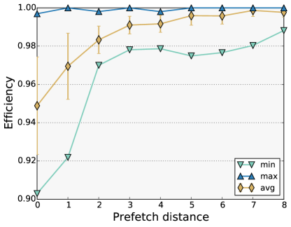
Figure 8: Minimum, average and maximum efficiency for a fixed prefetch distance across the benchmark.

4.4 Quality of Heuristics

On our Intel system, TTC evaluated roughly $8$ candidates per second across the whole benchmark (for tensors of size $200\text{\,}\mathrm{MB}$); this includes all the necessary steps from code-generation to compilation and measurement. If a solution has to be generated in a short period of time (i.e., the search space needs to be pruned efficiently), the quality of the heuristics to choose a proper loop order and blocking becomes especially important.

Fig. 9 presents the speedups that TTC achieves if the user limits the number of generated candidates to $1,10$ and $100$, and when no limit is given (i.e., $\infty$ reflects the same results as in Fig. 6(b) and 6(d)). When the number of generated candidates is limited to one, no search takes place, i.e., the loop order and the blocking for the generated implementation are determined solely by our heuristics. Even in this extreme case, TTC still exhibits remarkable speedups over modern compilers.

Specifically, with a search space of $1,10$ and $100$ candidates, TTC achieves $94.58\%,97.35\%$ and $99.10\%$ of the performance of the unlimited search (averaged across the whole benchmark). In other words, one can rely on the heuristics for the most part and resort to search only in scenarios in which even the last few bits of performance are critical. In those cases, we observe that a search space of $100$ candidates already yields results within $1$% from those obtained with an exhaustive search.

Figure 9: Speedup over the reference implementation with the number of TTC-generated candidates limited to $1,10,100$ and $\infty$ (i.e., no limit).

5 Conclusion and Future Work

We presented TTC, a compiler for multidimensional tensor transpositions. By deploying various optimization techniques, TTC significantly outperforms modern compilers, and achieves nearly optimal memory bandwidth. We investigated the source of the performance gain and illustrated the individual impact of blocking, software prefetching, explicit vectorization and loop-reordering. Furthermore, we showed that the heuristics used by TTC efficiently prune the search space, so that the remaining candidates are easily ranked via exhaustive search.

For the future, should compilation time become a concern, iterative compilation techniques should be considered [Kisuki et al. (2000), Knijnenburg et al. (2002)]. While this current work focused on architectures using the AVX instruction set, TTC is designed to accommodate other instruction sets; in general, the effort to port TTC to a new architecture is related to optimizations such as explicit vectorization and software prefetching. As a next step, we plan to support the AVX512 instruction set (e.g., used by Intel’s upcoming Knights Landing microarchitecture), ARM and IBM Power CPUs as well as NVIDIA GPUs. Finally, we will be using TTC as a building block for our upcoming Tensor Contraction Compiler.

Financial support from the Deutsche Forschungsgemeinschaft (DFG) through grant GSC 111 is gratefully acknowledged.

References

- [1]
- Abadi et al. (2015) Martın Abadi, Ashish Agarwal, Paul Barham, Eugene Brevdo, Zhifeng Chen, Craig Citro, Greg S Corrado, Andy Davis, Jeffrey Dean, Matthieu Devin, and others. 2015. TensorFlow: Large-scale machine learning on heterogeneous systems. (2015). https://www.tensorflow.org
- Bartlett and Musiał (2007) Rodney J. Bartlett and Monika Musiał. 2007. Coupled-cluster theory in quantum chemistry. Reviews in Modern Physics 79, 1 (2007), 291–352.
- Baumgartner et al. (2005) Gerald Baumgartner, Alexander Auer, David E Bernholdt, Alina Bibireata, Venkatesh Choppella, Daniel Cociorva, Xiaoyang Gao, Robert J Harrison, So Hirata, Sriram Krishnamoorthy, and others. 2005. Synthesis of high-performance parallel programs for a class of ab initio quantum chemistry models. Proc. IEEE 93, 2 (2005), 276–292.
- Chatterjee and Sen (2000) Siddhartha Chatterjee and S. Sen. 2000. Cache-efficient matrix transposition. (2000), 195–205. DOI:http://dx.doi.org/10.1109/HPCA.2000.824350
- Chetlur et al. (2014) Sharan Chetlur, Cliff Woolley, Philippe Vandermersch, Jonathan Cohen, John Tran, Bryan Catanzaro, and Evan Shelhamer. 2014. cuDNN: Efficient Primitives for Deep Learning. CoRR abs/1410.0759 (2014). http://arxiv.org/abs/1410.0759
- Di Napoli et al. (2014) Edoardo Di Napoli, Diego Fabregat-Traver, Gregorio Quintana-Ortí, and Paolo Bientinesi. 2014. Towards an efficient use of the BLAS library for multilinear tensor contractions. Appl. Math. Comput. 235 (2014), 454 – 468. DOI:http://dx.doi.org/10.1016/j.amc.2014.02.051
- Ding (2001) Chris HQ Ding. 2001. An optimal index reshuffle algorithm for multidimensional arrays and its applications for parallel architectures. Parallel and Distributed Systems, IEEE Transactions on 12, 3 (2001), 306–315.
- Dongarra et al. (1990) Jack J. Dongarra, Jermey Du Cruz, Sven Hammerling, and I. S. Duff. 1990. Algorithm 679: A Set of Level 3 Basic Linear Algebra Subprograms: Model Implementation and Test Programs. ACM Trans. Math. Softw. 16, 1 (March 1990), 18–28. DOI:http://dx.doi.org/10.1145/77626.77627
- Drake et al. (1995) John Drake, Ian Foster, John Michalakes, Brian Toonen, and Patrick Worley. 1995. Design and performance of a scalable parallel community climate model. Parallel Comput. 21, 10 (1995), 1571–1591.
- Finkel (2015) Hal Finkel. 2015. Optimizing for Blue Gene/Q. (2015). https://www.alcf.anl.gov/files/Optimizing_for_BGQ_rev.pdf
- Frigo and Johnson (2005) Matteo Frigo and Steven G. Johnson. 2005. The Design and Implementation of FFTW3. Proc. IEEE 93, 2 (Feb 2005), 216–231. DOI:http://dx.doi.org/10.1109/JPROC.2004.840301
- Gatlin and Carter (1999) Kang Su Gatlin and Larry Carter. 1999. Memory hierarchy considerations for fast transpose and bit-reversals. In High-Performance Computer Architecture, 1999. Proceedings. Fifth International Symposium On. IEEE, 33–42.
- Gauss et al. (1991) Jürgen Gauss, John F. Stanton, and Rodney J. Bartlett. 1991. Coupled‐cluster open‐shell analytic gradients: Implementation of the direct product decomposition approach in energy gradient calculations. The Journal of Chemical Physics 95, 4 (1991), 2623–2638. DOI:http://dx.doi.org/10.1063/1.460915
- Goldbogen (1981) Geoffrey C Goldbogen. 1981. PRIM: A fast matrix transpose method. IEEE Trans. Software Eng. 7, 2 (1981), 255–257.
- Hammond (2009) Jeff Hammond. 2009. Automatically tuned libraries for native-dimension tensor transpose and contraction algorithms. (2009). https://github.com/jeffhammond/spaghetty/blob/master/papers/old/spaghetty_chapter_v1.pdf
- Harrison et al. (2015) Robert J. Harrison, Gregory Beylkin, Florian A. Bischoff, Justus A. Calvin, George I. Fann, Jacob Fosso-Tande, Diego Galindo, Jeff R. Hammond, Rebecca Hartman-Baker, Judith C. Hill, Jun Jia, Jakob S. Kottmann, M.-J. Yvonne Ou, Laura E. Ratcliff, Matthew G. Reuter, Adam C. Richie-Halford, Nichols A. Romero, Hideo Sekino, William A. Shelton, Bryan E. Sundahl, W. Scott Thornton, Edward F. Valeev, Álvaro Vázquez-Mayagoitia, Nicholas Vence, and Yukina Yokoi. 2015. MADNESS: A Multiresolution, Adaptive Numerical Environment for Scientific Simulation. CoRR abs/1507.01888 (2015). http://arxiv.org/abs/1507.01888
- He and Ding (2002) Yun He and Chris HQ Ding. 2002. MPI and OpenMP paradigms on cluster of SMP architectures: the vacancy tracking algorithm for multi-dimensional array transposition. In Supercomputing, ACM/IEEE 2002 Conference. IEEE, 6–6.
- Hirata (2003) So Hirata. 2003. Tensor Contraction Engine: Abstraction and Automated Parallel Implementation of Configuration-Interaction, Coupled-Cluster, and Many-Body Perturbation Theories. Journal of Physical Chemistry A 107 (2003), 9887–9897.
- Intel Corporation (2015) Intel Corporation. 2015. Intel 64 and IA-32 architectures optimization reference manual. (2015). http://www.intel.com/content/dam/www/public/us/en/documents/manuals/64-ia-32-architectures-optimization-manual.pdf
- Jodra et al. (2015) Jose L Jodra, Ibai Gurrutxaga, and Javier Muguerza. 2015. Efficient 3D Transpositions in Graphics Processing Units. International Journal of Parallel Programming (2015), 1–16.
- Kisuki et al. (2000) Toru Kisuki, P Knijnenburg, M OBoyle, and H Wijshoff. 2000. Iterative compilation in program optimization. (2000), 35–44.
- Knijnenburg et al. (2002) Peter MW Knijnenburg, Toru Kisuki, and Michael FP OBoyle. 2002. Iterative compilation. In Embedded processor design challenges. Springer, 171–187.
- Kolda and Bader (2009) Tamara G Kolda and Brett W Bader. 2009. Tensor decompositions and applications. SIAM review 51, 3 (2009), 455–500.
- Kowalski et al. (2011) Karol Kowalski, Jeff R. Hammond, Wibe A. de Jong, Peng-Dong Fan, Marat Valiev, Dunyou Wang, and Niranjan Govind. 2011. Coupled Cluster Calculations for Large Molecular and Extended Systems. In Computational Methods for Large Systems: Electronic Structure Approaches for Biotechnology and Nanotechnology, Jeffrey R Reimers (Ed.). Wiley.
- Lee et al. (2012) Jaekyu Lee, Hyesoon Kim, and Richard W Vuduc. 2012. When Prefetching Works, When It Doesn’t, and Why. TACO 9, 1 (2012), 2.
- Li et al. (2015) Jiajia Li, Casey Battaglino, Ioakeim Perros, Jimeng Sun, and Richard Vuduc. 2015. An Input-adaptive and In-place Approach to Dense Tensor-times-matrix Multiply. In Proceedings of the International Conference for High Performance Computing, Networking, Storage and Analysis (SC ’15). ACM, New York, NY, USA, Article 76, 12 pages. DOI:http://dx.doi.org/10.1145/2807591.2807671
- Low et al. (2015) Tze Meng Low, Francisco D. Igual, Tyler M. Smith, and Enrique S. Quintana-Ortí. 2015. Analytical Models for the BLIS Framework. ACM Trans. Math. Software (2015). Pending.
- Lu et al. (2006) Qingda Lu, Sriram Krishnamoorthy, and P Sadayappan. 2006. Combining analytical and empirical approaches in tuning matrix transposition. In Proceedings of the 15th international conference on Parallel architectures and compilation techniques. ACM, 233–242.
- Lyakh (2015) Dmitry I Lyakh. 2015. An efficient tensor transpose algorithm for multicore CPU, Intel Xeon Phi, and NVidia Tesla GPU. Computer Physics Communications 189 (2015), 84–91.
- Markov and Shi (2008) Igor L Markov and Yaoyun Shi. 2008. Simulating quantum computation by contracting tensor networks. SIAM J. Comput. 38, 3 (2008), 963–981.
- Mateescu et al. (2012) Gabriel Mateescu, Gregory H Bauer, and Robert A Fiedler. 2012. Optimizing matrix transposes using a POWER7 cache model and explicit prefetching. ACM SIGMETRICS Performance Evaluation Review 40, 2 (2012), 68–73.
- McCalpin and Smotherman (1995) John McCalpin and Mark Smotherman. 1995. Automatic benchmark generation for cache optimization of matrix operations. In Proceedings of the 33rd annual on Southeast regional conference. ACM, 195–204.
- McCalpin (1995) John D. McCalpin. 1995. Memory Bandwidth and Machine Balance in Current High Performance Computers. IEEE Computer Society Technical Committee on Computer Architecture (TCCA) Newsletter (Dec. 1995), 19–25.
- Pekurovsky (2012) Dmitry Pekurovsky. 2012. P3DFFT: A framework for parallel computations of Fourier transforms in three dimensions. SIAM Journal on Scientific Computing 34, 4 (2012), C192–C209.
- Pfeifer et al. (2014) Robert NC Pfeifer, Jutho Haegeman, and Frank Verstraete. 2014. Faster identification of optimal contraction sequences for tensor networks. Physical Review E 90, 3 (2014), 033315.
- Solomonik et al. (2014) Edgar Solomonik, Devin Matthews, Jeff R Hammond, John F Stanton, and James Demmel. 2014. A massively parallel tensor contraction framework for coupled-cluster computations. J. Parallel and Distrib. Comput. 74, 12 (2014), 3176–3190.
- van Heel (1991) Marin van Heel. 1991. A fast algorithm for transposing large multidimensional image data sets. Ultramicroscopy 38, 1 (1991), 75–83.
- Vasilache et al. (2014) Nicolas Vasilache, Jeff Johnson, Michael Mathieu, Soumith Chintala, Serkan Piantino, and Yann LeCun. 2014. Fast convolutional nets with fbfft: A GPU performance evaluation. (2014). http://arxiv.org/abs/1412.7580
- Vladimirov (2013) Andrey Vladimirov. 2013. Multithreaded transposition of square matrices with common code for Intel Xeon processors and Intel Xeon Phi coprocessors. (2013). https://www.researchgate.net/profile/Andrey_Vladimirov/publication/258048110_Multithreaded_Transposition_of_Square_Matrices_with_Common_Code_for_Intel_Xeon_Processors_and_Intel_Xeon_Phi_Coprocessors/links/00463526c2fa40a1f3000000.pdf
- Wei and Mellor-Crummey (2014) Lai Wei and John Mellor-Crummey. 2014. Autotuning Tensor Transposition. In Parallel & Distributed Processing Symposium Workshops (IPDPSW), IEEE International. IEEE, 342–351.