Stock Selection as a Problem in Phylogenetics – Evidence from the ASX

Abstract

We report the results of fifteen sets of portfolio selection simulations using stocks in the ASX200 index for the period May 2000 to December 2013. We investigated five portfolio selection methods, randomly and from within industrial groups, and three based on neighbor-Net phylogenetic networks. We report that using random, industrial groups, or neighbor-Net phylogenetic networks alone rarely produced statistically significant reduction in risk, though in four out of the five cases in which it did so, the portfolios selected using the phylogenetic networks had the lowest risk. However, we report that when using the neighbor-Net phylogenetic networks in combination with industry group selection that substantial reductions in portfolio return spread were achieved.

Keywords:

Stock selection, ASX200, neighbor-Net networks, portfolio risk

JEL Codes:

G11

1 Introduction

Portfolio diversification is critical for risk management because it aims to reduce the variance of returns compared with a portfolio of a single stock or similarly undiversified portfolio. The academic literature on diversification is vast, stretching back at least as far as Lowenfeld (1909). The modern science of diversification is usually traced to Markowtiz (1952) which was expanded upon in great detail in Markowitz (1991).

In one sense, the approach of Markowtiz (1952) is optimal and cannot be improved in the case that, either the correlations and expected returns of the assets are not time-varying (thus can be accurately estimated from historical data) or, alternatively, they can be forecast accurately. Unfortunately, neither of these conditions hold in real markets leaving the door open to other approaches.

The literature covers a wide range of approaches to portfolio diversification, such as; the number of stocks required to form a well diversified portfolio, which has increased from eight stocks in the late 1960’s (Evans and Archer, 1968) to over 100 stocks in the late 2000’s (Domian et al., 2007), what types of risks should be considered, (Cont, 2001; Goyal and Santa-Clara, 2003; Bali et al., 2005), factors intrinsic to each stock (Fama and French, 1992; French and Fama, 1993), the age of the investor, (Benzoni et al., 2007), and whether international diversification is beneficial, (Jorion, 1985; Bai and Green, 2010), among others.

In recent years a significant number of papers have appeared which apply graph theoretical methods to the study of a stock or other financial market, see, for example, Mantegna (1999), Onnela et al. (2003a), Onnela et al. (2003b), Bonanno et al. (2004), Micciché et al. (2006), Naylor et al. (2007), Kenett et al. (2010), Djauhari (2012), and Rea and Rea (2014) among others.

On the pragmatic side, DiMiguel et al. (2009) list 15 different methods for forming portfolios and report results from their study which evaluated 13 of these. Absent among these 15 methods are any which utilize the above-mentioned graph theory approaches. This leaves an open question whether these graph theory approaches can usefully be applied to the problem of portfolio selection.

The goal of this paper is to compare three network methods with two simple portfolio selection methods for small private-investor sized portfolios. There are two motivations for looking at very small portfolios sizes.

The first is that, despite the recommendation of authorites like Domian et al. (2007), Barber and Odean (2008) reported that in a large sample of American private investors the average portfolio size of individual stocks was only 4.3. While comparable data does not appear to be available for private Australian investors, it seems unlikely that they hold substantially larger portfolios. Thus there is a practical need to find a way of maximising the diversification benefits for these investors. The second is that testing the methods on small portfolios gives us a chance to evaluate the potential benefits of the network methods because the larger the portfolio size, the more closely the portfolio resembles the whole market and the less any potential benefit is likely to be discernible.

The mean returns and variances of the individual contributing stocks are insufficient for making an informed decision on selecting a suite of stocks because selecting a portfolio requires an understanding of the correlations between each of the stocks available for consideration for inclusion in the portfolio. The number of correlations between stocks rises in proportion to the square of the number of stocks, meaning that for all but the smallest of stock markets the very large number of correlations is beyond the human ability to comprehend them. Rea and Rea (2014) presented a method to visualise the correlation matrix using nieghbor-Net networks (Bryant and Moulton, 2004), yielding insights into the relationships between the stocks.

Another key aspect of stock correlations is the potential change in the correlations with a significant change in market conditions (say comparing times of general market increase with recession and post-recession periods).

In this paper we explore investment opportunities on the Australian Stock Exchange using data from the stocks in the ASX200 index.

Our primary motivation is to investigate five portfolio selection strategies. The five strategies are;

1. picking stocks at random;

2. forming portfolios by picking stocks from different industry groups;

3. forming portfolios by picking stocks from different correlation clusters;

4. forming portfolios by picking stocks from the dominant industry group within correlation clusters;

5. forming portfolios by picking stocks from non-dominant industry groups within correlation clusters.

Our results show that knowledge of correlation clusters together with the industry groups within these clusters can reduce the portfolio risk.

The outline of this paper is as follows; Section (2) discusses the data and methods used in this paper, Section (3) discusses identifying the correlation clusters, Section (4) presents the results of the simulations of the portfolio selection methods and Section (5) contains the discussion and our conclusions.

2 Data and Methods

We used the weekly price data for the stocks in the ASX 200 as our dataset. Weekly prices along with the dividend rate and payment date for the period 3 May 2000 to 4 December 2013 were obtained from DataStream. We appended one or two letters to each ticker symbol in order to identify the industry group for each stock.

Weekly returns were calculated from the price and dividend data for use in both the portfolio formation simulations and for estimating the correlations. The correlations were estimated using the function cor in base R (R Core Team, 2014) We also calculated period returns for each stock in each of periods two to six for use in the simulations.

We divided the whole period into six shorter periods shown in Figure (1) and used out-of-sample testing to test the effectiveness of each the five methods of diversifying portfolios on reducing risk.

Figure 1: A plot of the ASX200 Index with the boundaries of the study periods marked.

2.1 Neighbor-Net Splits Graphs

To be able to use clustering algorithms (neighbor-Net is a clustering algorithm, Appendix (A) gives greater detail) we need to convert the numerical values in the correlation matrix to a measure which can be used as a distance. In the literature the most common way to do the conversion is by using the so-called ultra-metric given by,

$$d_{ij}=\sqrt{2(1-\rho_{ij})}$$ (1)

where $d_{ij}$ is the distance corresponding to the the estimated correlation, $\rho_{ij}$, between stocks $i$ and $j$, see Mantegna (1999) or Djauhari (2012) for details.

A typical stock market correlation matrix for $n$ stocks is of full rank which means that after converting to a distance matrix according to Equation (1), the location of the points, here stocks, can only be fully represented in $(n-1)$-dimensional space. In visualization, the high dimensional data space is collapsed to a sufficiently low dimensional space that the data can be represented on 2-dimensional surface such as a page or computer screen for viewing. Information loss is often unavoidable in the reduction of the dimension of the data space. One of the goals of visualization is to minimize the information loss while making the structures within the data visible to the human eye.

Using the conversion in Equation (1) we formatted the converted correlation matrix and augmented it with the appropriate stock codes for reading into the neighbor-Net software, SplitsTree, available from http://www.splitstree.org (Huson and Bryant, 2006). Using the SplitsTree software we generated the neighbor-Nets splits graphs. Because the splits graphs are intended to be used for visualization we defer the discussion of the identification of correlation clusters and their uses to Section (3) below.

2.2 Simulated Portfolios

Recently Lee (2011) discussed so-called risk-based asset allocation (sometimes called risk budgeting). In contrast to strategies which require both expected risk and expected returns for each investment opportunity as inputs to the portfolio selection process, risk-based allocation considers only expected risk. The five methods of portfolio selection we present below can be considered to be risk-based allocation methods. This probably reflects private investor behaviour in that often they have nothing more than broker buy, hold, or sell recommendations to assess likely returns.

The portfolio formation methods were compared using simulations of 1,000 iterations. There were two sets of simulations. For first set of simulations a portfolio was sampled based on the rules governing the portfolio type using the period return data. We recorded the mean and standard deviation of the returns for the 1,000 portfolios. The second set of simulations was carried out in exactly the same manner except weekly return data was used in order to obtain an estimate of the weekly volatility of the portfolios. Each set covered five portfolio formation strategies.

The five portfolio formation strategies are:

1. Selecting stocks at random;

2. Selecting stocks based on industry groupings;

3. Selecting stocks based on correlation clusters; and

4. Selecting stocks based on the dominant industry groups within the neighbor-Net correlation clusters.

5. Selecting stocks based on based on the non-dominant industry groups within the neighbor-Net correlation clusters.

We describe each of these in turn, combining (4) and (5) into a single description.

Random Selection:

The stocks were selected at random using a uniform distribution without replacement. In other words each stock was given equal chance of being selected according but with no stock being selected twice within a single portfolio.

By Industry Groups:

There were 11 industry groups represented among the stocks. Some of the groups were very small. For example, the telecommunications group only had two representatives in the early periods but this increased over time as additional stocks classified as being in the telecommunications industry were either listed or grew to sufficient size that they were included in the index. Thus, when the groups were small, it was necessary to merge some of them into larger groups for the purposes of the simulations. This need lessened as the number of stocks grew. We had eight such groups in periods two, three and four and nine groups in periods five and six.

Because the maximum portfolio size was eight stocks the industries were chosen at random using a uniform distribution without replacement. Within each industry group, stocks were selected using a uniform distribution.

By Correlation Clusters:

The correlation clusters were determined by examining the neighbor-Net network for the relevant periods (periods one through five). Each stock was assigned to exactly one cluster and each cluster can be defined by a single split (or bipartition) of the circular ordering of the neighbor-Net for the relevant period. The clusters determined in periods one through five were used to generate the stock groups for out-of-sample testing in periods two through six respectively. Because the goal of portfolio building is to reduce risk each cluster was paired with another cluster which was considered most distant from it. This method is discussed in detail below.

If there were fewer clusters than the desired portfolio size, cluster pairs were selected at random and a stock selected from within each correlation cluster pair. The simulation code was written so that if the desired portfolio size was larger than the number of correlation clusters then each cluster group pair had at least $s$ stocks selected, where $s$ is the quotient of the portfolio size divided by the number of clusters. Some (the remainder of the portfolio size divided by number of clusters) correlation groups will have $s+1$ stocks selected and the cluster pairs this applied to were chosen using a uniform distribution without replacement. However, in all cases the number of clusters equalled or exceeded the number of stocks in the simulated portfolios.

By Dominant or Non-Dominant Industry Group within Clusters:

The final two methods relate to selecting stocks from industry groups within correlation clusters. Each stock within each cluster has an associated industry group. Therefore each correlation cluster can be subdivided into up to eleven sub-clusters based on industry. However, it was clear that in a number of clusters one industry was dominant, sometimes more than half of the stocks. This lead us to assign each stock to either the dominant industry group or the non-dominant industry grouping creating two groups of stocks within each cluster. This created two disjoint sets of clusters with no stock in both groups.

From these two distinct sets of stocks, simulations were run in the same manner as that described in “By Correlation Clusters” above. These simulations were not comparable with the three above because the sample sizes were different and, obviously, each deals with a subset of the data. However, care was taken to ensure that the sample sizes of both subsets was as close to equal in size as was practical.

A problem arose, particularly with the non-dominant industry group stocks when the number of stocks in the cluster was considered too small. In these cases we took advantage of the circular ordering produced by neighbor-Nets and combined the small cluster with a neighbouring cluster.

Unchanged from above, each cluster was paired with the one most distant from it. Once a cluster was selected for inclusion, so was the paired cluster, and a selection was made using a uniform distribution and, if necessary, without replacement.

All simulations were coded and run in R (R Core Team, 2014).

We used the stocks’ weekly return data in period one to determine the clusters, then observed period two’s return distributions of the simulated portfolios (1000 replications) which are picked from the different correlation clusters. Because out-of-sample testing was used in our analysis, the simulation then was continued for period three, four, five and six based on the graphs produced from the weekly returns in period two, three, four and five respectively.

3 Neighbor-Net Splits Graphs

For three of the five types of portfolio simulation methods discussed above we need to identify correlation clusters from the neighbor-Net splits graphs. In this section we explain how to identify the clusters, then proceed to present the neighbor-Net splits graphs and the clusters identified for each of the first five periods.

At its simplest a neighbor-Net splits graph is a type of map. The ability to identify correlation clusters depends on the user’s skill in reading it. As an analogy, all readers of a topographic map read the map in the same way. The information the reader extracts depends on their needs. One person may read a map to extract information about mountain ranges, another for information on river catchments, and still another on the distribution of human settlements. But in all cases the map readers agree which features are mountains, which are rivers and which are towns and cities, no confusion arises because the map is read visually. In the same way all readers of neighbor-Net splits graphs agree on which feature or features are the origin, which are splits, which are recombinations and which are the terminal locations.

Because this is a visual approach, the information extracted from reading a neighbor-Net splits graph depends on the researcher or financial analyst balancing whatever competing requirements they may have. Here we know that in the simulations to follow the sizes of the portfolios we will generate will be two, four, or eight stocks. Consequently, we do not need large numbers of clusters and we would like them to have a sufficiently large number of stocks such that when selecting stocks at random from within the cluster there are a sufficiently large number of combinations available to make the simulations meaningful. These requirements guide us when identifying clusters in the neighbor-Net splits graphs. The numbers of clusters and cluster membership is determined visually and it is important not to confuse visual with subjective.

Figures (2) through (8) present the neighbor-Nets splits graphs for periods one through five. These were used to determine the stock groups for out-of-sample testing using data from periods two through six respectively.

In Figure (2) eight clusters were identified and are colour coded in order to distinguish them. The SplitsTree software generates a large amount of statistical information about the network. However, we, like other users of neighbor-Nets, look for breaks in the structure of the network. A good example can be found at about eight o’clock in the splits graph between the stocks labelled CMW_F and CPA_F. In its original context of phylogenetics, if these were species it would tell us that the last common ancestor was in the distant past. Although CMW_F and CPA_F are placed next to each other in the circular ordering, the two stocks are not closely related.

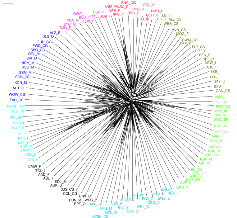
Figure 2: Period 1 neighbor-Nets splits graph with eight clusters identified.

Figure (3) presents the same splits graph but within each cluster the stocks are split into stocks which belong to the dominant industry group (larger typeface) and stocks which are in other groups (smaller typeface). For example, in the aqua coloured group, the dominant industry is financials and all but three stocks belong to this sector.

Figure 3: Period 1 neighbor-Nets splits graph with the clusters split into dominant and non-dominant industries.

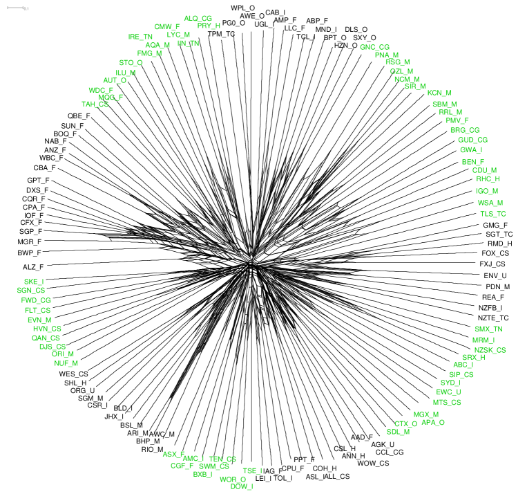
Figure 4: Period 2 neighbor-Nets splits graph with 10 clusters.

Figure (4) presents the neighbor-Nets splits graph for period 2. While the clusters in this figure have not been visually separated into dominant and non-dominate industry groups, the cluster between nine and ten o’clock is dominated by financial stocks. It is also straight-forward to see how the clusters were paired. The cluster just mentioned would be paired with the black coloured cluster between about 2:30 and 3:30 on the opposite side of the network. These stocks are the most distant in terms of the circular ordering. If the correlation clusters represent useful financial groupings of stocks we would expect that choosing a pair of stocks from these two clusters would be likely to give a greater reduction in risk than two stocks selected randomly.

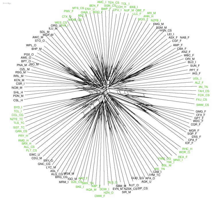
Figure 5: Period 3 neighbor-Nets splits graph with 10 clusters.

Figure (5) gives a good example of where the cluster pairing may be different. Consider the green coloured cluster at the top of the splits graph. It is relatively large and we shall call it cluster one. At the bottom of the graph are three smaller clusters, two black and one green coloured which we shall call clusters six, seven and eight, reading the circular ordering in a clockwise direction. The most distant cluster from cluster one (the cluster at 12 o’clock) would be cluster seven (the green coloured cluster at six o’clock). However, we should pair both clusters six and seven (the black coloured cluster at five o’clock and the green coloured cluster at six o’clock respectively) with cluster one. This illustrates the fact that while all clusters have a cluster they are paired with, not all clusters are a reciprocal pair.

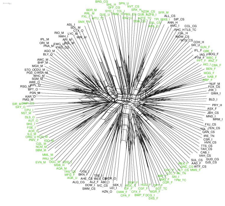
Figure 6: Period 4 neighbor-Nets splits graph with eight clusters.

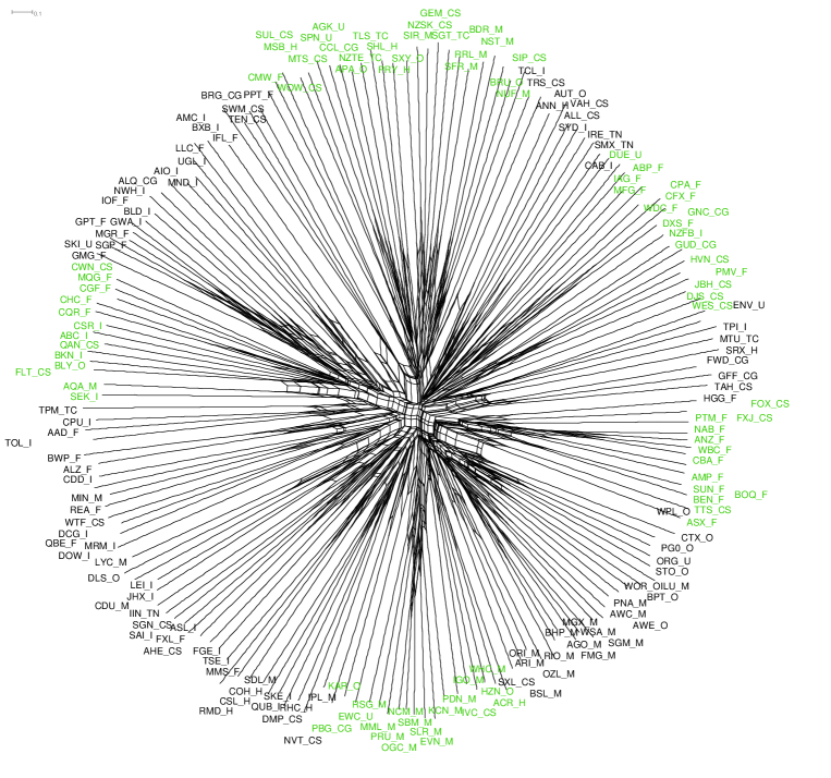
Figure 7: Period 5 neighbor-Nets splits graph with 10 clusters.

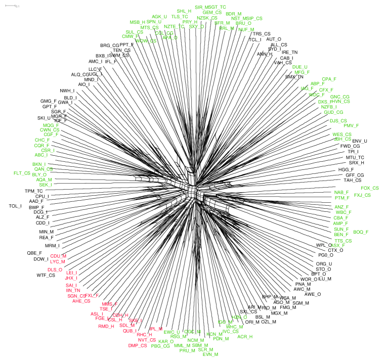
Figure 8: Period 5 neighbor-Nets splits graph with 11 clusters. Cluster 5 in Figure (7) has been split into two smaller clusters coloured red and black.

Figures (7) and (8) are both splits graphs for period 5 divided into 10 and 11 correlation clusters respectively. As the number of stocks included in the analysis grows the analyst gains some flexibility in choosing the number of clusters.

To summarize, a stock market analyst or portfolio manager looks for breaks in the structure of the neighbor-Net network when dividing the stocks into correlation clusters. The SplitsTree software has considerable flexibility to magnify sections of the network to aid in decision making which cannot be easily captured in the static pdf file outputs included in this paper. The circular ordering can be very useful when splitting a correlation cluster into its component industry groups because if one or more of the resulting groups are too small to be useful they can be joined with groups next to them in the circular order.

4 Results

Tables (1) through (5) together with Figures (9) though (13) present the results of the portfolio selection simulations.

In the third part of each table we have labelled the results presented there the “Sharpe Ratio” though this is clearly not the ratio of Sharpe (1964). The Sharpe ratio is properly applied to single assets or single portfolios and estimates the reward to risk ratio. Here were are dividing the mean portfolio return by the standard deviation of the returns estimated from the replications. A higher ratio indicates either a higher mean return or a lower spread of returns generated by that selection method or some combination of both. We believe the results are worth reporting but do not discuss them further in this paper.

Period 2		Neighbor-Net’s	Industry	Correlation	Correlation
Simulation	Random	correlation	Group	cluster with	cluster without
results		cluster		industry group	industry group
Mean return
(2-stock)	106.49	94.93	98.52	101.80	97.24
(4-stock)	101.51	98.45	96.93	97.55	97.12
(8-stock)	104.66	96.90	100.82	98.892	96.14
Std. Dev.
(2-stock)	79.34	*70.51	73.87	81.90	*62.47
(4-stock)	*49.39	51.85	48.96	53.14	*43.62
(8-stock)	*33.61	35.64	36.56	42.33	*29.81
Sharpe Ratio
(2-stock)	1.34	1.35	1.33	1.24	1.56
(4-stock)	2.06	1.90	1.98	1.84	2.23
(8-stock)	3.11	2.72	2.69	2.70	3.23
Levene Tests
(2-stock)			0.001		$1.0\times 10^{-7}$
(4-stock)			0.30		$1.7\times 10^{-6}$
(8-stock)			0.13		$1.3\times 10^{-12}$

Table 1: Period 2 portfolio performances with standard deviation for three different portfolio sizes. The selection method with the lowest standard deviation is marked with an asterisk (*). The neighbor-Nets method is out-of-sample testing using the correlation clusters determined from Period 1 data. The first Levene test is the p-value whether the standard deviation of the three different portfolio selection methods are equal. The second result is for the neightbor-Net clusters split into dominant and non-dominant industry groupings.

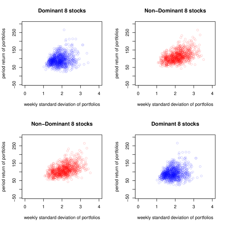
Figure 9: Scatter plots of Period 2 returns against the weekly volatility for the eight-stock portfolios selected on the basis of the clusters identified in neighbor-Nets splits graph from Period 1 with the clusters split into dominant and non-dominant industry groups.

Table (1) presents the results for the Period 2 simulations which was a period of strongly rising equity prices. The model building period (Period 1) was a period when the market largely tracked sideways with a small decline over the period. Thus the out-of-sample test represents a strong test of stock selection methods between the two periods which do not resemble each other.

We are primarily concerned with reducing the risk of the portfolios. The results in the table give the standard deviation of the returns of the 1000 replications of the portfolio selection method. A lower standard deviation indicates that the returns of the portfolios were more concentrated about the mean portfolio return. The Levene tests show that only the two stock portfolios had a significantly different spread of returns. The difference between the random selection method and neighbor-Nets selection was almost nine percentage points different.

The final two columns of Table (1) present the results for the simulations in which the correlation clusters were divided into dominant and non-dominant industry groups. In this case the correlation clusters of non-dominant industries showed statistically significantly lower levels of spread of the portfolio returns.

Figure (9) plots the returns of the weekly standard deviation of the portfolio returns, a measure of volatility, against the period portfolio return for the eight-stock portfolios dividing the stocks in to dominant and non-dominant industry groups. The differences are not pronounced but the spread of returns is smaller for the correlation clusters with non-dominant industry groups though the weekly volatility appears comparable.

Period 3		Neighbor-Net’s	Industry	Correlation	Correlation
Simulation	Random	correlation	Group	cluster with	cluster without
results		cluster		industry group	industry group
Mean return
(2-stock)	156.32	149.30	135.11	137.09	150.97
(4-stock)	152.99	151.27	134.02	132.85	155.49
(8-stock)	154.30	149.05	137.79	134.82	152.94
Std. Dev.
(2-stock)	108.11	109.64	*99.57	*66.02	116.40
(4-stock)	75.93	75.47	*71.01	*45.62	83.45
(8-stock)	51.34	50.15	*48.26	*32.49	57.63
Sharpe Ratio
(2-stock)	1.45	1.36	1.36	2.07	1.27
(4-stock)	2.01	2.00	1.89	2.91	1.86
(8-stock)	3.01	2.97	2.86	4.15	2.65
Levene Tests
(2-stock)			0.05		$<10^{-16}$
(4-stock)			0.15		$<10^{-16}$
(8-stock)			0.06		$<10^{-16}$

Table 2: Period 3 portfolio performances with standard deviation for three different portfolio sizes. The selection method with the lowest standard deviation is marked with an asterisk (*). The neighbor-Nets method is out-of-sample testing using the correlation clusters determined from Period 2 data. The first Levene test is the p-value whether the standard deviation of the three different portfolio selection methods are equal. The second result is for the neightbor-Net clusters split into dominant and non-dominant industry groupings.

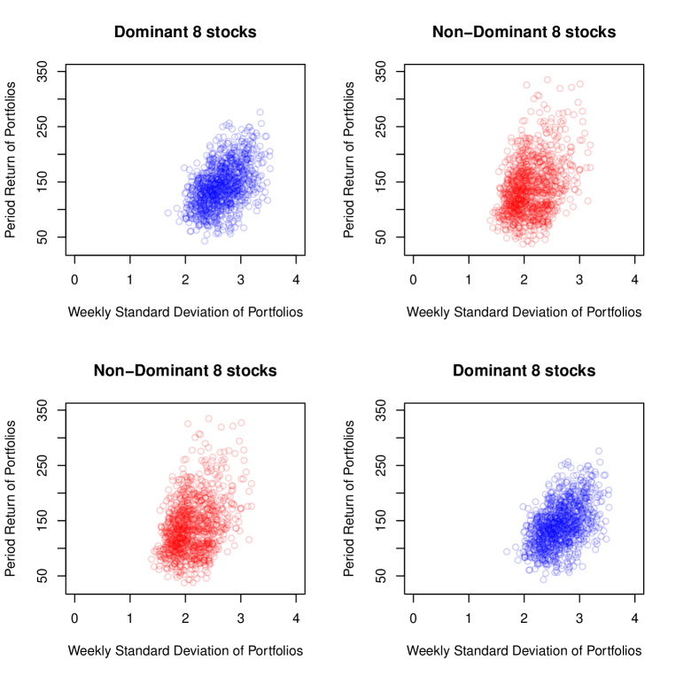
Figure 10: Scatter plots of Period 3 returns against the weekly volatility for the eight-stock portfolios selected on the basis of the clusters identified in neighbor-Nets splits graph from Period 2 with the clusters split into dominant and non-dominante industry groups.

Table (2) presents the results for the Period 3 simulations which was a period of strongly rising equity prices. The model building period (Period 2) was also a period of market increases. Thus the out-of-sample test and model building periods closely resemble each other.

The Levene tests show that only the two stock portfolios had a significantly different spread of returns, though the results for the eight-stock portfolios almost reached statistical significance. The difference between the neighbor-Nets selection and industry group selection was almost 10 percentage points different.

The final two columns of Table (2) present the results for the simulations in which the correlation clusters were divided into dominant and non-dominant industry groups. In this case the correlation clusters of the dominant industries showed statistically significantly lower levels of spread of the portfolio returns.

Figure (10) plots the returns of the weekly standard deviation of the portfolio returns, a measure of volatility, against the period portfolio return for the eight-stock portfolios dividing the stocks in to dominant and non-dominant industry groups. It is noticeable that the spread of returns is smaller for the correlation clusters with dominant industry groups though the weekly volatility is higher.

Period 4		Neighbor-Net’s	Industry	Correlation	Correlation
Simulation	Random	correlation	Group	cluster with	cluster without
results		cluster		industry group	industry group
Mean return
(2-stock)	-46.58	-49.18	-45.56	-54.61	-43.26
(4-stock)	-47.52	-49.46	-43.93	-54.81	-42.19
(8-stock)	-47.48	-48.52	-44.09	-54.70	-42.18
Std. Dev.
(2-stock)	22.80	*21.30	21.70	*17.16	23.49
(4-stock)	*15.16	15.41	15.68	*11.29	16.80
(8-stock)	10.65	10.49	*10.42	*8.03	11.11
Sharpe Ratio
(2-stock)	-2.04	-2.31	-2.10	-3.18	-1.85
(4-stock)	-3.13	-3.21	-2.80	-4.85	-2.51
(8-stock)	-4.46	-4.62	-4.25	-6.81	-3.80
Levene Tests
(2-stock)			0.78		$1.6\times 10^{-9}$
(4-stock)			0.32		$<10^{-16}$
(8-stock)			0.73		$<10^{-16}$

Table 3: Period 4 portfolio performances with standard deviation for three different portfolio sizes. The selection method with the lowest standard deviation is marked with an asterisk (*). The neighbor-Nets method is out-of-sample testing using the correlation clusters determined from Period 3 data. The first Levene test is the p-value whether the standard deviation of the three different portfolio selection methods are equal. The second result is for the neightbor-Net clusters split into dominant and non-dominant industry groupings.

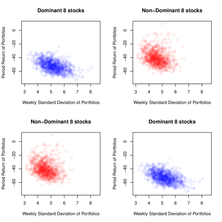
Figure 11: Scatter plots of Period 4 returns against the weekly volatility for the eight-stock portfolios selected on the basis of the clusters identified in neighbor-Nets splits graph from Period 3 with the clusters split into dominant and non-dominant industry groups.

Table (3) presents the result for the Period 4 simulations. Period four was a period of strongly falling equity prices. The model building period (Period 3) was a period of strong market increases. Thus the out-of-sample test and model building periods are effectively opposites of each other.

The Levene tests show that no stock portfolios had a significantly different spread of returns.

The final two columns of Table (3) present the results for the simulations in which the correlation clusters were divided into dominant and non-dominant industry groups. In this case the correlation clusters of the dominant industries showed statistically significantly lower levels of spread of the portfolio returns. The Levene tests were highly significant for all portfolio sizes.

Figure (11) plots the returns of the weekly standard deviation of the portfolio returns against the period portfolio return for the eight-stock portfolios dividing the stocks in to dominant and non-dominant industry groups. It is noticeable that the spread of returns is substantially smaller for the correlation clusters with dominant industry groups though, again, the weekly volatility is higher.

Period 5		Neighbor-Net’s	Industry	Correlation	Correlation
Simulation	Random	correlation	Group	cluster with	cluster without
results		cluster		industry group	industry group
Mean return
(2-stock)	164.49	159.20	156.22	142.77	160.07
(4-stock)	162.29	150.17	160.37	149.74	164.06
(8-stock)	162.43	154.90	162.25	151.25	163.34
Std. Dev.
(2-stock)	144.70	149.58	*141.50	*124.24	155.57
(4-stock)	105.14	*94.92	99.47	*83.90	106.43
(8-stock)	70.68	*68.04	70.61	*60.30	73.00
Sharpe Ratio
(2-stock)	1.14	1.06	1.10	1.15	1.03
(4-stock)	1.54	1.58	1.61	1.78	1.54
(8-stock)	2.30	2.28	2.38	2.51	2.24
Levene Tests
(2-stock)			0.46		$3.9\times 10^{-5}$
(4-stock)			0.003		$3.3\times 10^{-8}$
(8-stock)			0.35		$1.4\times 10^{-8}$

Table 4: Period 5 portfolio performances with standard deviation for three different portfolio sizes. The selection method with the lowest standard deviation is marked with an asterisk (*). The neighbor-Nets method is out-of-sample testing using the correlation clusters determined from Period 4 data. The first Levene test is the p-value whether the standard deviation of the three different portfolio selection methods are equal. The second result is for the neightbor-Net clusters split into dominant and non-dominant industry groupings.

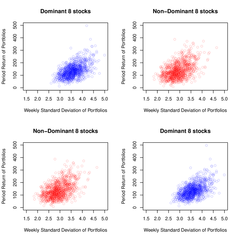
Figure 12: Scatter plots of Period 5 returns against the weekly volatility for the eight-stock portfolios selected on the basis of the clusters identified in neighbor-Nets splits graph from Period 4 with the clusters split into dominant and non-dominant industry groups.

Table (4) presents the results for the Period 5 simulations which was a period of equity prices initially rebounding then tracking sideways. The model building period (Period 4) was a period of strong market decreases. Thus the out-of-sample test and model building periods are substantially different.

The Levene tests show that only the four stock portfolios had a significantly different spread of returns.

The final two columns of Table (4) present the results for the simulations in which the correlation clusters were divided into dominant and non-dominant industry groups. In this case the correlation clusters of the dominant industries showed statistically significantly lower levels of spread of the portfolio returns. The Levene tests were strongly significant for all portofilos sizes.

Figure (12) plots the returns of the weekly standard deviation of the portfolio returns against the period portfolio return for the eight-stock portfolios dividing the stocks in to dominant and non-dominant industry groups. It is noticeable that the spread of returns is smaller for the correlation clusters with dominant industry groups though, again, the weekly volatility is higher.

Period 6		Neighbor-Net’s	Industry	Correlation	Correlation
Simulation	Random	correlation	Group	cluster with	cluster without
results		cluster		industry group	industry group
Mean return
(2-stock)	45.96	46.60	54.36	34.77	65.16
(4-stock)	48.39	51.10	55.19	35.85	61.87
(8-stock)	46.66	50.32	55.62	35.36	62.09
Std. Dev.
(2-stock)	52.03	*49.87	51.62	*44.92	51.32
(4-stock)	37.28	*33.18	34.11	*28.49	35.65
(8-stock)	25.56	*21.63	22.94	*15.04	24.04
Sharpe Ratio
(2-stock)	0.88	0.93	1.05	0.77	1.27
(4-stock)	1.30	1.54	1.62	1.26	1.74
(8-stock)	1.76	2.33	2.42	2.35	2.58
Levene Tests
(2-stock)			0.64		0.004
(4-stock)			0.007		$4.0\times 10^{-9}$
(8-stock)			$1.1\times 10^{-9}$		$<10^{-16}$

Table 5: Period 6 portfolio performances with standard deviation for three different portfolio sizes. The selection method with the lowest standard deviation is marked with an asterisk (*). The neighbor-Nets method is out-of-sample testing using the correlation clusters determined from Period 5 data. The first Levene test is the p-value whether the standard deviation of the three different portfolio selection methods are equal. The second result is for the neightbor-Net clusters split into dominant and non-dominant industry groupings.

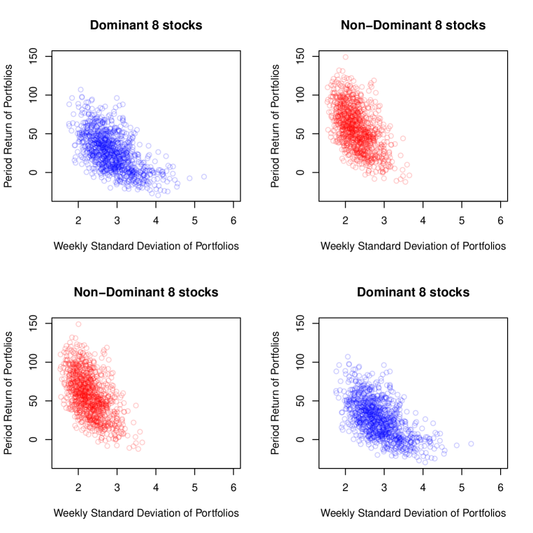
Figure 13: Scatter plots of Period 6 returns against the weekly volatility for the eight-stock portfolios selected on the basis of the clusters identified in neighbor-Nets splits graph from Period 5 with the clusters split into dominant and non-dominant industry groups.

Table (5) presents the result for the Period 6 simulations which was a period of rising equity prices with significant volatility. The model building period (Period 5) was a period of rebound followed by a time of stacking sideways. Thus the out-of-sample test and model building periods have some similarities.

The Levene tests show that the four and eight stock portfolios had a significantly different spread of returns. In both cases the neighbor-Nets portfolio selection method had the lowest spread of returns.

The final two columns of Table (5) present the results for the simulations in which the correlation clusters were divided into dominant and non-dominant industry groups. In this case the correlation clusters of the dominant industries showed statistically significantly lower levels of spread of the portfolio returns. The Levene tests were highly significant for all portofilos sizes.

Figure (13) plots the returns of the weekly standard deviation of the portfolio returns against the period portfolio return for the eight-stock portfolios dividing the stocks in to dominant and non-dominant industry groups. It is noticeable that the spread of returns is smaller for the correlation clusters with dominant industry groups though, as with some previous periods, the weekly volatility is higher.

5 Discussion and Conclusions

The simulation tests performed here represent a particularly severe test of portfolio diversification because of the long out-of-sample test periods coupled with the fact that the market conditions in the model building phase were often very different from the market conditions in the test phase.

In the 15 sets of simulations comparing, random, industry group, and neighbor-Net correlation cluster selection methods, statistically significant differences in the portfolios standard deviation were obtained only five times. In four cases the neighbor-Net correlation cluster produced the lowest standard deviation and in one case the industry group selection method was the lowest.

Considering the neighbor-Net correlation clusters split into dominant and non-dominant industries, all 15 cases had statistically significant differences in the portfolios’ standard deviation. Of these 12 were correlation clusters with dominant industry groups in Periods 3 through 6 and three were correlation clusters with non-dominant industry groups in Period 2. Because we do not have data from before the inception date of the ASX200 index it is not possible to say if this represents a change in the behaviour of the market.

Figures (9) through (13) present this last observation in graphical form and it is clear that the distribution both in terms of portfolio returns and weekly volatility are different for all periods. Graphs of the two and four stock portfolios show similar results but are not reported here.

These results suggest that within each correlation cluster there are two distinct sub-populations of stocks. Intuitively, the dominant industry group are simply stocks within the same industry with similar risk characteristics. We would expect such stocks to be strongly correlated, hence fall into the same correlation cluster. We would also expect that they would continue to be strongly correlated into the future. On the other hand, the stocks in the non-dominant industry group within a correlation cluster would seem far less likely to remain strongly correlated in the future.

At this stage we can only recommend that this be investigated further. The differences between the two groups of stocks appear significant both in a statistical and economic sense but it is not yet clear how to exploit this difference for financial gain.

This paper is primarily concerned about reducing risk in small portfolios. However, investors are also concerned about returns and in three of the five periods (two, three and five) the randomly selected portfolios had the highest returns among the three methods which included all stocks. Truly negative correlations among stocks are uncommon and in a strongly rising market a negative correlation between a pair of stocks often indicates that one stock is suffering from some form of financial distress and hence a falling share price. The correlation cluster method excludes many stock combinations available to the random selection method but also increases the probability of a stock being paired with one in financial distress hence depressing overall portfolio performance. If this explanation is correct then the application of financial analysis aimed at removing financially distressed stocks may well enhance the performance of all portfolio selection methods. Again, this must wait for further research.

Appendix A Neighbor-Net

This appendix gives a more technical description of the Neighbor-Net algorithm.

The construction of Neighbor-Net networks has four key components: the agglomerative process, selection formulae, distance reduction and estimation of the split weights. The agglomerative process describes how the hierarchy of nodes is determined, selection formulae describe the system used in determining the hierarchy and distance reduction describes how the distances are adjusted as the hierarchy is built. The result of the these three steps is a circular collection of splits. Formally a set of circular splits is one which satisfies that condition that there is an ordering of the nodes $x_{1},x_{2},\ldots,x_{n}$ such that every split is of the form $\{x_{i},x_{i+1},\ldots,x_{j}\}|X-\{x_{i},\ldots,x_{j}\}$ for some $i$ and $j$ satisfying $1\leq i\leq j<n$. As highlighted above, the advantage of this set of splits is that they can be represented on a plane.

We describe the algorithm following Bryant and Moulton (2004). All the nodes start out as singletons and the selection formulae finds the two closest nodes. These nodes are not grouped immediately but remain as singletons until a node has two neighbors. At this stage the three nodes, the node and its two neighbors, are merged into two nodes. Here we present the selection formula for grouping nodes. Let neighboring relations group the $n$ nodes into $m$ clusters. Let $d_{xy}$ be the distance between nodes $x$ and $y$. Let $C_{1},C_{2},\ldots,C_{m},m\leq n$ be the $m$ clusters. The distance $d(C_{i},C_{j})$ between two clusters is

$$d(C_{i},C_{j})=\frac{1}{|C_{i}||C_{j}|}\sum_{x\in C_{i}}\sum_{y\in C_{j}}d_{xy},$$ (2)

that is, an average of the distances between elements in each cluster.

The closest pair of clusters is given by finding the $i$ and $j$ that minimise

$$Q(C_{i},C_{j})=(m-2)d(C_{i},C_{j})-\sum_{k=i,k\neq i}{m}d(C_{i},C_{k})-\sum_{k=i,k\neq i}{m}d(C_{j},C_{k}),$$ (3)

and denote them $C_{i*}$ and $C_{j*}$

To choose particular nodes within clusters we select the node from each cluster that minimises

$$\hat{Q}(x_{i},x_{j})=(\hat{m}-2)d(x_{i},x_{j})-\sum_{k=i,k\neq i}{\hat{m}}d(x_{i},C_{k})-\sum_{k=i,k\neq i}{\hat{m}}d(x_{j},C_{k})$$ (4)

where $x_{i}\in C_{i*}$ and $x_{j}\in C_{j*}$ and $\hat{m}=m+|C_{i*}|+|C_{j*}|-2$.

The distance reduction updates the distance matrix with the distance from the two new clusters to all the other clusters. The distance reduction formulae calculate the distances between the existing nodes and the new combined nodes. If $y$ has two neighbors, $x$ and $z$, then the three nodes will be combined and replaced by two nodes which we can denote as $u$ and $v$. The Neighbor-Net algorithm uses

$$d(u,a) = (\alpha+\beta)d(x,a)+\gamma d(y,a)$$ (5)

$$d(v,a) = \alpha d(y,a)+(\beta+\gamma)d(z,a)$$ (6)

$$d(u,v) = \alpha d(x,y)+\beta d(x,z)+\gamma d(y,z)$$ (7)

where $\alpha,\beta$ and $\gamma$ are non-negative real numbers with $\alpha+\beta+\gamma=1$.

The process stops when all the nodes are in a single cluster.

The Neighbor-Net method of Bryant and Moulton (2004) used non-negative least squares to estimate the split weights given the distance vector and a set splits known as the circular splits. Suppose that the splits in the network are numbered $1,2,\ldots,m$ and that the nodes are numbered $1,2,\ldots,n$. Let $\mathbf{X}$ be the be the splits matrix with the dimensions $n(n-1)/2\times m$ matrix with rows indexed by pairs of nodes, columns indexed by splits, and entry $\mathbf{X}_{ij,k}$ given by

$$\mathbf{X}_{ij,k} = \begin{cases}1\text{ if $i$ and $j$ are on opposite sides of the split}\\ 0\text{ if $i$ and $j$ are on the same side of the split.}\end{cases}$$ (8)

Similar nodes will be clustered together in the network. This is a direct result of each pair of neighboring nodes in the ordering being close together in terms of distance, and separated from node where the distance measure reveals dissimilarity.

The network, or splits graph, generated by Neighbor-Nets has three biologically meaningful components. The places where a line splits represents a speciation event, where a single population becomes two genetically isolated populations. The places where two lines join to become one represents a recombination event, where two genetically isolated populations exchange genetic material. The lengths of the indivdual lines represent the time the population evolves without either a speciation or recombination event. The interpretation of these three components in a financial context is an active area of research for the authors.

References

- Bai and Green (2010) Bai, Y. and C. J. Green (2010). International Diversification Strategies: Revisited from the Risk Perspective. The Journal of Banking and Finance 34, 236–245.
- Bali et al. (2005) Bali, T. G., N. Cakici, X. Yan, and Z. Zhang (2005). Does Idiosyncratic Risk Really Matter? The Journal of Finance 60(2), 905–929.
- Barber and Odean (2008) Barber, B. M. and T. Odean (2008). All That Glitters: The Effect of Attention and News on the Buying Behaviour of Individual and Institutional Investors. The Review of Financial Studies 21(2), 785–818.
- Benzoni et al. (2007) Benzoni, L., P. Collin-Dufresne, and R. S. Goldstein (2007). Portfolio Choice over the Life-Cycle when the Stock and Labor Markets are Cointegrated. The Journal of Finance 62(5), 2123–2167.
- Bonanno et al. (2004) Bonanno, G., G. Calderelli, F. Lillo, S. Micciché, N.Vandewalle, and R. N. Mantegna (2004). Networks of equities in financial markets. The European Physical Journal B 38, 363–371. doi:10.1140/epjb/e2–4-00129-6.
- Bryant and Moulton (2004) Bryant, D. and V. Moulton (2004). Neighbor-net: An agglomerative method for the construction of phylogenetic networks. Molecular Biology and Evolution 21(2), 255–265.
- Cont (2001) Cont, R. (2001). Empirical properties of asset returns: stylized facts and statistical issues. Quantitative Finance 1:2, 223–236.
- DiMiguel et al. (2009) DiMiguel, V., L. Garlappi, and R. Uppal (2009). Optimal versus Naive Diversification: How Inefficient is the 1/N Portfolio Strategy? Review of Financal Studies 22(5), 1915–1953.
- Djauhari (2012) Djauhari, M. A. (2012). A Robust Filter in Stock Networks Analysis. Physica A 391(20), 5049–5057.
- Domian et al. (2007) Domian, D. L., D. A. Louton, and M. D. Racine (2007). Diversification in Portfolios of Individual Stocks: 100 Stocks Are Not Enough. The Financial Review 42, 557–570.
- Evans and Archer (1968) Evans, J. L. and S. H. Archer (1968). Diversification and the Reduction of Dispersion: An Empirical Analysis. The Journal of Finance 23(5), 761–767.
- Fama and French (1992) Fama, E. F. and K. R. French (1992). The Cross-Section of Expected Stock Returns. The Journal of Finance 47(2), 427–465.
- French and Fama (1993) French, K. R. and E. F. Fama (1993). Common Risk Factors in the Returns on Stocks and Bonds. Journal of Financal Economics 33, 3–56.
- Goyal and Santa-Clara (2003) Goyal, A. and P. Santa-Clara (2003). Idiosyncratic Risk Matters! The Journal of Finance 58(3), 975–1007.
- Huson and Bryant (2006) Huson, D. H. and D. Bryant (2006). Application of phylogenetic networks in evolutionary studies. Molecular Biology and Evolution 23(2), 255–265.
- Jorion (1985) Jorion, P. (1985). International Portfolio Diversification with Estimation Risk. The Journal of Business 58(3), 259–278.
- Kenett et al. (2010) Kenett, D. Y., M. Tumminello, A. Madi, G. Gur-Gershgoren, R. N. Mantegna, and E. Ben-Jacob (2010). Systematic analysis of group identification in stock markets. PLoS ONE 5, e15032.
- Lee (2011) Lee, W. (2011). Risk-Based Asset Allocation: A New Answer to an Old Question? Journal of Portfolio Management 37(4), 11–28.
- Lowenfeld (1909) Lowenfeld, H. (1909). Investment, an Exact Science. Financial Review of Reviews.
- Mantegna (1999) Mantegna, R. N. (1999). Hierarchical structure in financial markets. The European Physical Journal B 11, 193–197.
- Markowitz (1991) Markowitz, H. M. (1991). Portfolio Selection: Efficient Diversification of Investments 2nd Edition. Wiley.
- Markowtiz (1952) Markowtiz, H. (1952). Portfolio Selection. The Journal of Finance 7(1), 77–91.
- Micciché et al. (2006) Micciché, S., G. Bonannon, F. Lillo, and R. N. Mantegna (2006). Degree stability of a minimum spanning tree of price return and volatility. Physica A 324, 66–73.
- Naylor et al. (2007) Naylor, M. J., L. C. Rose, and B. J. Moyle (2007). Topology of foreign exchange markets using hierarchical structure methods. Physica A 382, 199–208.
- Onnela et al. (2003a) Onnela, J.-P., A. Chakraborti, K. Kaski, J. Kertèsz, and A. Kanto (2003a). Asset Trees and Asset Graphs in Financial Markets. Physica Scripta T106, 48–54.
- Onnela et al. (2003b) Onnela, J.-P., A. Chakraborti, K. Kaski, J. Kertèsz, and A. Kanto (2003b). Dynamics of market correlations: Taxonomy and portfolio analysis. Physical Review E 68, 0561101–1 – 056110–12.
- R Core Team (2014) R Core Team (2014). R: A Language and Environment for Statistical Computing. Vienna, Austria: R Foundation for Statistical Computing.
- Rea and Rea (2014) Rea, A. and W. Rea (2014). Visualization of a stock market correlation matrix. Physica A 400, 109–123.
- Sharpe (1964) Sharpe, W. F. (1964). Capital Asset Prices: A Theory of Market Equilibrium Under Conditions of Risk. The Journal of Finance 19(3), 13–37.