Emergence of massless Dirac quasiparticles in correlated hydrogenated graphene with broken sublattice symmetry

Abstract

Using the variational cluster approximation (VCA) and the cluster perturbation theory, we study the finite temperature phase diagram of a half-depleted periodic Anderson model on the honeycomb lattice at half filling for a model of graphone, i.e., single-side hydrogenated graphene. The ground state of this model is found to be ferromagnetic (FM) semi-metal. The origin of this FM state is attributed to the instability of a flat band located at the Fermi energy in the noninteracting limit and is smoothly connected to the Lieb-Mattis type ferromagnetism. The spin wave dispersion in the FM state is linear in momentum at zero temperature but becomes quadratic at finite temperatures, implying that the FM state is fragile against thermal fluctuations. Indeed, our VCA calculations find that the paramagnetic (PM) state dominates the finite temperature phase diagram. More surprisingly, we find that massless Dirac quasiparticles with the linear energy dispersion emerge at the Fermi energy upon introducing the electron correlation $U$ at the impurity sites in the PM phase. The Dirac Fermi velocity is found to be highly correlated to the quasiparticle weight of the emergent massless Dirac quasiparticles at the Fermi energy and monotonically increases with $U$. These unexpected massless Dirac quasiparticles are also examined with the Hubbard-I approximation and the origin is discussed in terms of the spectral weight redistribution involving a large energy scale of $U$. Considering an effective quasiparticle Hamiltonian which reproduces the single-particle excitations obtained by the Hubbard-I approximation, we argue that the massless Dirac quasiparticles are protected by the electron correlation. Our finding is therefore the first example of the emergence of massless Dirac quasiparticles due to dynamical electron correlations without breaking any spatial symmetry. The experimental implications of our results for graphone as well as a graphene sheet on transition metal substrates are also briefly discussed.

I Introduction

Graphene Novoselov2005 has been one of the most actively studied research subjects in current condensed matter physics Neto2009RMP . Although its unique electronic property is characterized already in a single-particle level, namely, with the linear electronic energy dispersion, i.e., the Dirac cone dispersion, at the Fermi energy ($E_{\rm F}$) Wallace1947 , many-body effects on graphene have also attracted much attention Kotov2012 . For example, tremendous efforts have been devoted on investigating whether a spin liquid state can exist in the half-filled Hubbard model on the honeycomb lattice Meng2010 ; Sorella2012 ; Assaad2013 , one of the simplest models for graphene, and the nature of metal-insulator transition Toldin2015 ; Otsuka2015 .

The research has been also extended to graphene derived systems, e.g., a series of hydrogenated graphene Sofo2007 ; Elias2009 ; Ray2014 ; Peng2014 . A first-principles calculation based on density functional theory (DFT) has predicted that the single-side hydrogenated graphene, called graphone, becomes a ferromagnetic (FM) semiconductor with a small indirect gap Zhou2009 . Other DFT based study has suggested that the single-side hydrogenated and fluorinated graphenes are both candidates for quantum spin liquid Rudenko2013 . Possible increase of the spin-orbit coupling due to the $sp^{3}$ lattice distortion has been also discussed Neto2009 ; Gmitra2013 .

Many-body effects on the hydrogenated graphene, however, have not been explored so far. On the one hand, the isolated graphene, described by, e.g., the single-band Hubbard model on the honeycomb lattice Schuler2013 , remains semi-metallic even when a moderate amount of electron interactions are introduced before the antiferromagnetic instability sets in Meng2010 ; Sorella2012 ; Assaad2013 ; Sorella1992 , and thus the correlation effect in semi-metallic phase is merely renormalization Otsuka2015 . On the other hand, the electron correlation in the hydrogen atoms should be treated in a many-body way, as suggested in the Heitler-London description for the chemical bonding of a hydrogen molecule HL . It is also noteworthy that many-body effects on hydrogen atoms in metal can induce a Kondo-like effect and make a drastic correction in the single-particle excitation spectrum as compared with that obtained by DFT calculations Eder1997 .

Here, we employ the variational cluster approximation (VCA) Potthoff2003 and the cluster perturbation theory (CPT) Senechal2000 to investigate many-body effects on graphone by considering a half-depleted periodic Anderson model on the honeycomb lattice at half filling. We find that the ground state of this model is FM semi-metallic. The FM state is attributed to the instability of a flat band located at $E_{\rm F}$ in the noninteracting limit and smoothly connected to the Lieb-Mattis type ferromagnetism. The liner spin wave analysis of an effective spin model for the periodic Anderson model in the strong coupling limit finds that the spin wave excitations in the FM state exhibits the linear dispersion in momentum at zero temperature, while the spin wave dispersion becomes quadratic at finite temperatures, implying that the FM state is fragile against thermal fluctuations and can be stable only at zero temperature.

Our VCA calculations indeed find that the finite temperature phase diagram is dominated by a paramagnetic (PM) state. Most significantly, we find that massless Dirac quasiparticles emerge at $E_{\rm F}$ upon introducing the electron correlation in the PM phase. The Dirac Fermi velocity of the emergent massless Dirac quasiparticles is found to be highly correlated to the quasiparticle weight at the Fermi energy and increase monotonically with the electron correlation. We show that the emergence of the massless Dirac quasiparticles is well captured by the simple Hubbard-I approximation and can be understood as the result of the spectral weight redistribution involving a large energy scale of the electron correlation. By considering an effective Hamiltonian for the quasiparticles, we discuss the chiral symmetry of the single-particle excitations in the PM phase within the Hubbard-I approximation and argue that the emergent massless Dirac quasiparticles are protected by the electron correlation. The massless Dirac quasiparticles found here in the PM phase are therefore in sharp contrast to massless Dirac dispersions generated by band engineering with breaking a crystalline symmetry, and represent the first example of the emergence of massless Dirac quasiparticles induced by dynamical electron correlations.

The rest of this paper is organized as follows. Sec. II introduces the periodic Anderson model studied here and explains briefly the numerical methods, i.e., the VCA and the CPT. These numerical methods are employed to obtain the finite temperature phase diagram and examine the single-particle excitations in Sec. III. The results are compared with those obtained analytically using the mean-field theory in Sec. IV.1 and the Hubbard-I approximation in Sec. IV.2. An effective Hamiltonian for the quasiparticles is constructed on the basis of the Hubbard-I approximate analysis and the chiral symmetry of the quasiparticle excitations is discussed in Sec. IV.3. The implications of our results for experiments are also briefly discussed in Sec. V before summarizing the paper in Sec. VI.

In addition, five appendices are provided to supplement the main text. The stability of the FM state is examined with the liner spin wave theory in Appendix A. Lieb’s theorem is applied to the periodic Anderson model in Appendix B. This analysis, together with the numerically exact diagonalization study of small clusters in Appendix C, reveals that the FM ground state found here is smoothly connected to the Lieb-Mattis type ferromagnetism. The single-particle excitations for several limiting cases are also examined within the Hubbard-I approximation in Appendix D. Finally, the Brillouin-Wigner perturbation theory is applied to the effective quasiparticle Hamiltonian in Appendix E.

II Model and Methods

In this section, we first introduce a periodic Anderson model as one of the simplest models for graphone, i.e., single-side hydrogenated graphene, and summarize the electron band structure of this model in the noninteracting limit. Next, we briefly explain the finite temperature VCA and CPT to treat the electron correlation effect on the finite temperature phase diagram and the single-particle excitations beyond the single-particle approximation.

II.1 Periodic Anderson model

We consider a half-depleted periodic Anderson model on the honeycomb lattice defined as

$$\mathcal{H}=\mathcal{H}_{0}+\epsilon_{H}\sum_{i}\sum_{\sigma}n_{\mathbf{r}_{i}\sigma H}+U\sum_{i}n_{\mathbf{r}_{i}\uparrow H}n_{\mathbf{r}_{i}\downarrow H},$$ (1)

where

$$\mathcal{H}_{0} = -t\sum_{i}\sum_{\sigma}\sum_{{\bm{\delta}}}\left(c_{\mathbf{r}_{i}\sigma A}^{\dagger}c_{\mathbf{r}_{i}+{\bm{\delta}}\sigma B}+{\rm h.c.}\right)$$ (2)

$$+ t_{sp}\sum_{i}\sum_{\sigma}\left(c_{\mathbf{r}_{i}\sigma B}^{\dagger}c_{\mathbf{r}_{i}\sigma H}+\mathrm{h.c.}\right),$$

$c^{\dagger}_{\mathbf{r}_{i}\sigma\alpha}$ is the electron creation operator with spin ${\sigma\,(=\uparrow,\downarrow)}$ and orbital $\alpha$ (= $A$, $B$, and $H$) in the $i$-th unit cell locating at $\mathbf{r}_{i}$, and $n_{\mathbf{r}_{i}\sigma\alpha}=c^{\dagger}_{\mathbf{r}_{i}\sigma\alpha}c_{\mathbf{r}_{i}\sigma\alpha}$. Here, orbital $A$ ($B$) denotes carbon $p_{z}$ orbital on $A$ ($B$) sublattice of the honeycomb lattice and orbital $H$ indicates hydrogen $s$ orbital (see Fig. 1). The conduction band of the periodic Anderson model is described by the first term of Eq. (2), where the hopping integral $t$ is finite only between the nearest-neighboring carbon sites, indicated by the sum over ${\bm{\delta}}=(0,0)$, $\mathbf{d}_{1}$, and $\mathbf{d}_{2}$ with $\mathbf{d}_{1}=\left(1/2,\sqrt{3}/2\right)a$ and $\mathbf{d}_{2}=\left(-1/2,\sqrt{3}/2\right)a$ being the primitive translational vectors of the honeycomb lattice ($a$: the lattice constant between the next nearest-neighboring carbon sites). The hybridization between the conduction band in the graphene plane and the hydrogen “impurity” sites is denoted by $t_{sp}$, where each hydrogen impurity site is linked only with the carbon site on $B$ sublattice, as shown in Fig. 1. The on-site potential energy and the on-site Coulomb repulsion at the hydrogen impurity sites are denoted by $\epsilon_{H}$ and $U$, respectively.

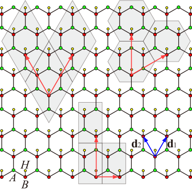
Figure 1: (color online) Schematic honeycomb lattice structure on which the half-depleted periodic Anderson model is defined for a model of graphone, i.e., single-side hydrogenated graphene. Green and red circles denote the carbon conduction sites on $A$ and $B$ sublattices of the honeycomb lattice, respectively, and yellow circles indicate the hydrogen impurity sites. The primitive translational vectors of the honeycomb lattice, $\mathbf{d}_{1}=\left(\frac{1}{2},\frac{\sqrt{3}}{2}\right)a$ and $\mathbf{d}_{2}=\left(-\frac{1}{2},\frac{\sqrt{3}}{2}\right)a$, are denoted by blue arrows, where $a$ is the lattice constant between the next nearest-neighboring carbon sites. Clusters considered in the VCA and the CPT (grey shaded regions) include a 12-site cluster containing 4 unit cells (upper left), a 9-site cluster containing 3 unit cells (upper right), and a 6-site cluster containing 2 unit cells (lower center). The orange arrows indicate primitive translational vectors for each cluster. The 6-site and 9-site clusters are used for finite temperature calculations and the 12-site cluster is used for zero temperature calculations.

The periodic Anderson model $\mathcal{H}$ described in Eq. (1) is the simplest model for graphone, implicitly assuming that the hopping integral $t$ in the conduction band should be considered as the renormalized one due to the electron correlation in the carbon sites. In the following, we set the electron density $n$ to be one for any $U$ at all temperatures by imposing the particle-hole symmetry with $\epsilon_{H}=-U/2$, and thus the local electron density in each site is exactly one. We also set $a=\hbar=k_{B}=1$.

II.2 Noninteracting limit

In the noninteracting limit with $\epsilon_{H}=0$, the Hamiltonian leads in the momentum space

$$\mathcal{H}_{0}=\sum_{\mathbf{k},\sigma}\mathbf{c}^{\dagger}_{\mathbf{k}\sigma}\left(\begin{array}[]{ccc}0&\gamma_{\mathbf{k}}&0\\ \gamma^{*}_{\mathbf{k}}&0&t_{sp}\\ 0&t_{sp}&0\end{array}\right)\mathbf{c}_{\mathbf{k}\sigma},$$ (3)

where $\mathbf{c}^{\dagger}_{\mathbf{k}\sigma}=(c_{\mathbf{k}\sigma A}^{\dagger}\,c_{\mathbf{k}\sigma B}^{\dagger}\,c_{\mathbf{k}\sigma H}^{\dagger})$ is the Fourier transform of the real space creation operators and

$$\gamma_{\mathbf{k}}=-t\left(1+e^{i\mathbf{k}\cdot\mathbf{d_{1}}}+e^{i\mathbf{k}\cdot\mathbf{d_{2}}}\right).$$ (4)

The characteristic features are summarized as follows (see also Fig. 2): (i) The Dirac cone dispersions which are present for the pure graphene model are now absent, (ii) instead, the massive Dirac dispersions, described as $E_{\mathbf{k}}=\pm\sqrt{|\gamma_{\mathbf{k}}|^{2}+t_{sp}^{2}}$, appear near $K$ and $K^{\prime}$ points, and (iii) in addition there exists the flat band at $E_{\rm F}$, i.e., $E_{\mathbf{k}}=0$, which is composed of $A$ and $H$ orbitals (solely of $A$ orbital at $K$ and $K^{\prime}$ points), but not $B$ orbital. Note also that the flat band is exactly half-filled at $n=1$.

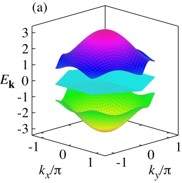
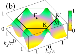
Figure 2: (color online) (a) The energy band structure $E_{\mathbf{k}}$ (in unit of $t$) and (b) $\langle\phi_{{\mathbf{k}}\sigma}^{\rm flat}|c^{\dagger}_{{\mathbf{k}}\sigma A}c_{{\mathbf{k}}\sigma A}|\phi_{{\mathbf{k}}\sigma}^{\rm flat}\rangle$ for the noninteracting case with $t_{sp}/t=1$, where $|\phi_{\mathbf{k}\sigma}^{\rm flat}\rangle$ is the eigenstate of the flat band with $E_{\mathbf{k}}=0$ at momentum $\mathbf{k}=(k_{x},k_{y})$. The first Brillouin zone is indicated by the hexagon with solid lines in (b), where high symmetric momenta are also denoted by $\Gamma$: $(0,0)$, $K$: $\frac{4\pi}{3a}(1,0)$, $K^{\prime}$: $\frac{4\pi}{3a}(\frac{1}{2},\frac{\sqrt{3}}{2})$, and $M$: $\frac{4\pi}{3a}(\frac{3}{4},\frac{\sqrt{3}}{4})$.

The features (i), (ii) and (iii) are understood by noticing that ${\cal H}_{0}$ satisfies the Lieb’s condition on a bipartite lattice with no hopping between the same sublattices Lieb . Following Lieb’s argument, ${\cal H}_{0}$ has $|A|+|H|-|B|$ ($|\alpha|$: the number of $\alpha$ orbitals) zero eigenvalues, forming the flat band, and the wave functions with zero eigenvalues are contributed only from $A$ and $H$ orbitals. The simplified tight binding model considered here already captures the main characteristic features obtained by spin-unpolarized DFT calculations, including the almost dispersionless band near $E_{\rm F}$ with almost zero weight of hydrogen orbitals around $K$ and $K^{\prime}$ points Zhou2009 ; Rudenko2013 .

II.3 Variational cluster approximation

We employ the VCA Potthoff2003 to investigate a possible symmetry broken magnetic ordered state. Here, we introduce, as a variational parameter, a uniform field $h^{\prime}$ on the hydrogen impurity sites Horiuchi2008 described as

$$\mathcal{H}_{h^{\prime}}=h^{\prime}\sum_{i}\left(n_{\mathbf{r}_{i}\uparrow H}-n_{\mathbf{r}_{i}\downarrow H}\right).$$ (5)

The reference system $\mathcal{H}_{\rm ref}$ considered is thus composed of $\mathcal{H}_{h^{\prime}}$ and a collection of disconnected finite size clusters, as shown in Fig. 2 (a), where each cluster is described by $\mathcal{H}$ but with no hopping terms between clusters, the corresponding Hamiltonian being denoted as $\mathcal{H}_{\rm c}$. Hence, the reference system is described as $\mathcal{H}_{\rm ref}=\mathcal{H}_{\rm c}+\mathcal{H}_{h^{\prime}}$.

The VCA evaluates as a function of $h^{\prime}$ the grand potential functional

$$\mathcal{F}=\frac{1}{L_{\mathrm{c}}}\mathcal{F}^{\prime}-\frac{T}{NL_{\mathrm{c}}}\sum_{\sigma}\sum_{\omega_{\nu}}\sum_{\mathbf{\tilde{k}}}\ln\det\left[\boldsymbol{I}-\boldsymbol{V}_{\sigma}(\mathbf{\tilde{k}})\boldsymbol{G}_{\sigma}^{\prime}(\mathrm{i}\omega_{\nu})\right],$$ (6)

where $\omega_{\nu}=(2\nu+1)\pi T$ with an integer $\nu$ is the Matsubara frequency for a given temperature $T$ and the wave vector $\mathbf{\tilde{k}}$ is defined in the reduced Brillouin zone of the reference system. The reference system $\mathcal{H}_{\rm ref}$ comprises $N$ identical clusters and each cluster contains $L_{\rm c}$ unit cells. The single-particle Green’s function of a single cluster in $\mathcal{H}_{\rm ref}$ is denoted as $\boldsymbol{G}^{\prime}_{\sigma}(i\omega_{\nu})$. $\boldsymbol{V}_{\sigma}(\mathbf{\tilde{k}})$ is the $(3L_{\rm c}\times 3L_{\rm c})$ sub-matrix element of block-diagonalized $\boldsymbol{V}$ in the momentum ($\mathbf{\tilde{k}}$) and spin ($\sigma$) spaces, where $\boldsymbol{V}$ is a matrix representation of the one-body Hamiltonian $\mathcal{H}_{\rm ref}-\mathcal{H}$. ${\boldsymbol{I}}$ is the $(3L_{\rm c}\times 3L_{\rm c})$ unit matrix. The grand potential $\mathcal{F}^{\prime}$ of the single cluster is readily evaluated as

$$\mathcal{F}^{\prime}=-T\ln\sum_{s}\exp(-E_{s}/T),$$ (7)

where $E_{s}$ is the $s$-th eigenvalue of a single cluster in $\mathcal{H}_{\rm ref}$. The exact diagonalization method is employed to obtain $\boldsymbol{G}_{\sigma}^{\prime}(i\omega_{\nu})$ and $\mathcal{F}^{\prime}$ numerically exactly. The FM state is obtained when a saddle point $\partial\mathcal{F}/\partial h^{\prime}|_{h^{\prime}=h^{*}}=0$ with the lowest $\mathcal{F}$ is at $h^{*}\not=0$.

II.4 Cluster perturbation theory

The CPT Senechal2000 is employed to obtain the translationally invariant single-particle Green’s function of the infinite system. In the CPT, the single-particle Green’s function $\mathcal{G}^{\alpha\beta}_{\sigma}(\mathbf{k},z)$ of $\mathcal{H}$ is given as

$$\mathcal{G}^{\alpha\beta}_{\sigma}(\mathbf{k},z)=\frac{1}{L_{c}}\sum_{i,j}\left(\boldsymbol{G}^{\prime-1}_{\sigma}(z)-\boldsymbol{V}_{\sigma}(\mathbf{k})\right)_{i\alpha,j\beta}^{-1}e^{-i\mathbf{k}\cdot(\mathbf{r}_{i}-\mathbf{r}_{j})},$$ (8)

where $\alpha$ and $\beta$ are orbital indices (i.e., $A$, $B$, and $H$ orbitals) and the sums over $i$ and $j$ are for unit cells within a single cluster in $\mathcal{H}_{\rm ref}$. The single-particle Green’s function $\boldsymbol{G}^{\prime}_{\sigma}(z)$ of the single cluster is obtained within the VCA, as described above. Note here that the momentum $\mathbf{k}$ and the complex frequency $z$ can take any values. Therefore, we can achieve arbitrarily fine resolution of $\mathbf{k}$ and $z$ for the single-particle excitations, which allows us for the detailed analysis of the spectral properties including the spectral weight and the Dirac Fermi velocity.

III Numerical results

In this section, we first discuss the finite temperature phase diagram of the periodic Anderson model obtained by the VCA. Next, we examine in details the single-particle excitations in each phase of the phase diagram using the CPT.

III.1 Phase diagram

The finite temperature phase diagram obtained by the VCA is summarized in Fig. 3. We find that the ground state is always FM semi-metallic for $U>0$ and the magnetic moment

$$m_{z}=\frac{1}{NL_{\rm c}}\sum_{i}\sum_{\alpha}\left(\langle n_{\mathbf{r}_{i}\uparrow\alpha}\rangle-\langle n_{\mathbf{r}_{i}\downarrow\alpha}\rangle\right)$$ (9)

is exactly one, where $\langle\cdots\rangle$ implies the thermal average. Thus, strictly speaking, the ground state is ferrimagnetic seki2015 . As discussed above in Sec. II.2, in the noninteracting limit with $U=0$, the flat band exists exactly at $E_{\rm F}$ and is half-filled [see Fig. 2(a)]. Therefore, the system is unstable against FM order upon introducing $U$. We assign the origin of this FM state to be flat-band ferromagnetism Titvinidze . It should be also noted that, in the strong coupling limit where an electron in each hydrogen impurity site is completely localized, the Ruderman-Kittel-Kasuya-Yoshida (RKKY) interaction RKKY between these localized spins is FM Saremi2007 (see also Appendix A.1), which naturally induces the FM ground state.

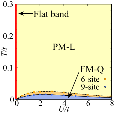
Figure 3: (color online) Finite temperature phase diagram of the periodic Anderson model $\mathcal{H}$ obtained by the VCA for the 6-site and 9-site clusters with $t_{sp}/t=1$ at $n=1$. PM-L (FM-Q) stands for a PM (FM) phase with the linear (quadratic) quasiparticle dispersion around $E_{\rm F}$. In the noninteracting limit with $U=0$, the flat band appears at $E_{\rm F}$ (red solid line). The FM state is stable in a blue (orange) shaded region below a solid (dashed) line for the 9-site (6-site) cluster.

As discussed in Appendix B, Lieb’s theorem itself Lieb does not guarantee the uniqueness of the ground state of $\mathcal{H}$. This is simply because there is no on-site interaction $U_{C}$ for the carbon conduction sites in $\mathcal{H}$. However, numerically exactly diagonalizing small clusters, we find in Appendix C that in the parameter region studied here the ground state for $U_{C}\neq 0$ is smoothly connected to the non-degenerate ground state for $U_{C}=0$ (apart from the trivial spin degeneracy), implying that the ground state of $\mathcal{H}$ is the Lieb-Mattis type ferromagnetism on a bipartite lattice with total spin $S=(|A|+|H|-|B|)/2$ LM .

With increasing the temperature, however, the FM state is thermally destroyed and a PM state becomes stable. Notice here that the finite FM critical temperature $T_{\rm C}$ found in the VCA is due to a mean-field like treatment of the electron correlation beyond the size of clusters. Indeed, increasing the size of a cluster from 6 sites to 9 sites, we find that $T_{\rm C}$ decreases for all values of $U/t$, as shown in Fig. 3. In Appendix A, we also analyze with the linear spin wave theory an effective spin Hamiltonian for the periodic Anderson model in the strong coupling limit, and find that the spin wave dispersion $\Omega_{\mathbf{q}}$ with momentum ${\mathbf{q}}$ around $\Gamma$ point is proportional to $|{\mathbf{q}}|$ at $T=0$ but $|{\mathbf{q}}|^{2}$ at finite temperatures (see Fig. 19 and 20), implying that the FM order is stable only at $T=0$, as is expected from Mermin-Wagner theorem Mermin1966 Therefore, the finite $T_{\rm C}$ obtained in the VCA should be regarded as a temperature where the short range FM correlations are developed over the size of a cluster, and the finite temperature phase diagram is dominated by the PM phase.

As shown below, it is more surprising to find in the PM phase that massless Dirac quasiparticles emerge at $K$ and $K^{\prime}$ points with the Dirac points exactly at $E_{\rm F}$.

III.2 Single-particle excitations

The single-particle excitation spectrum

$$A^{\alpha\beta}_{\sigma}(\mathbf{k},\omega)=-\frac{1}{\pi}\Im\mathcal{G}^{\alpha\beta}_{\sigma}(\mathbf{k},\omega+i\eta)$$ (10)

can be easily obtained from the single-particle Green’s function $\mathcal{G}^{\alpha\beta}_{\sigma}({\mathbf{k}},z)$ calculated using the CPT in Eq. (8). Here, $\omega$ is the real frequency and $\eta$ is real positive infinitesimal for Lorentzian broadening of the spectrum.

III.2.1 FM ground state

Figure 4 shows the typical results of the single-particle excitation spectrum in the FM ground state for $U/t=4$ at $T=0$. The enlarged spectrum close to the Fermi energy $E_{\rm F}$ around $K$ point is also shown in Fig. 5. It is clearly observed in Fig. 5 that (i) the low-energy single-particle excitations around $E_{\rm F}$ display the quadratic energy dispersion in momentum, indicating massive quasiparticle excitations, and (ii) the lowest single-particle excitations around $K$ point (and also $K^{\prime}$ point) are composed mostly of $A$ orbital (the lowest excitations at $K$ and $K^{\prime}$ points are solely due to $A$ orbital and their spectral weights are independent of $U$). The latter is the remnant to the noninteracting case shown in Fig. 2(b).

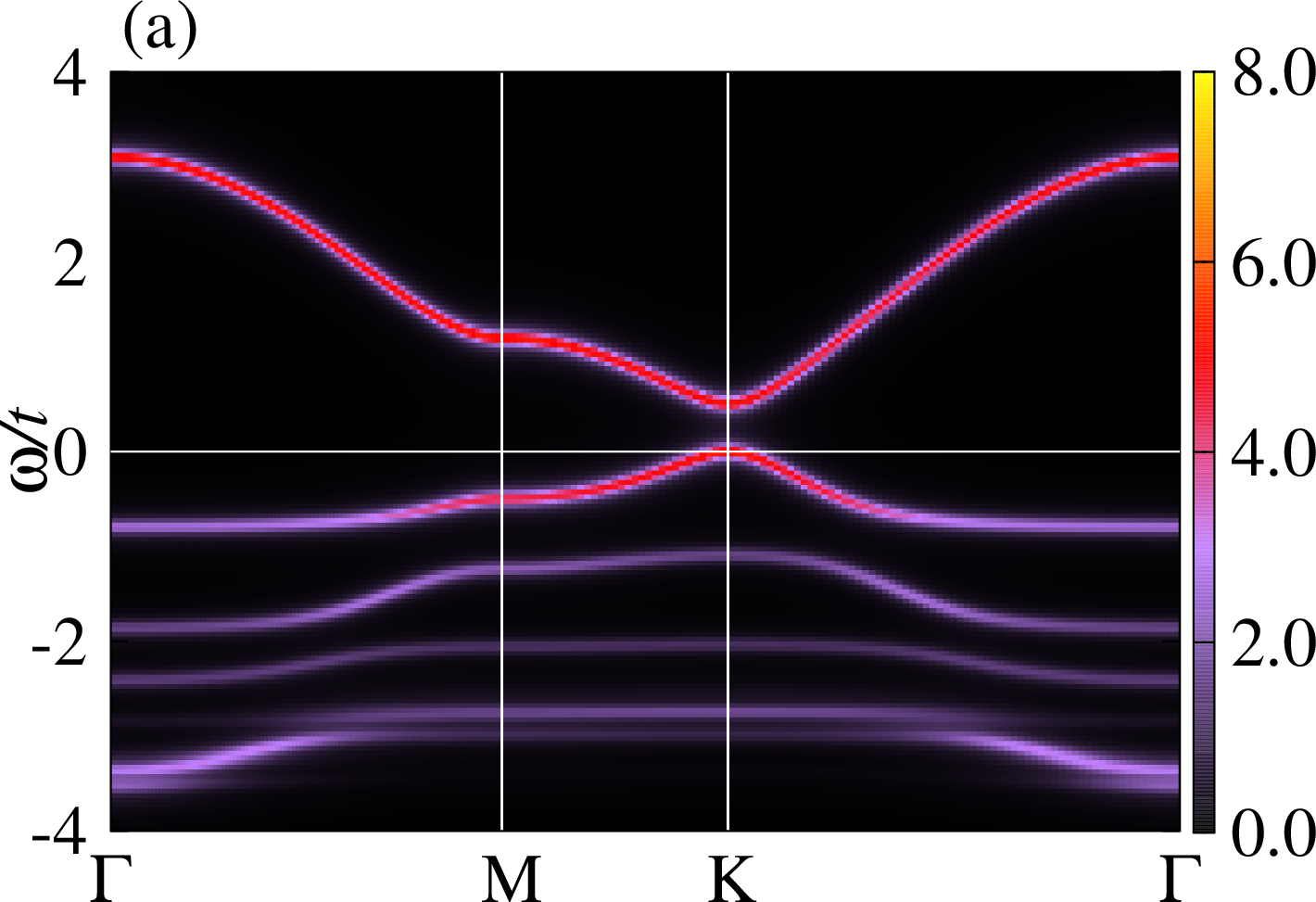
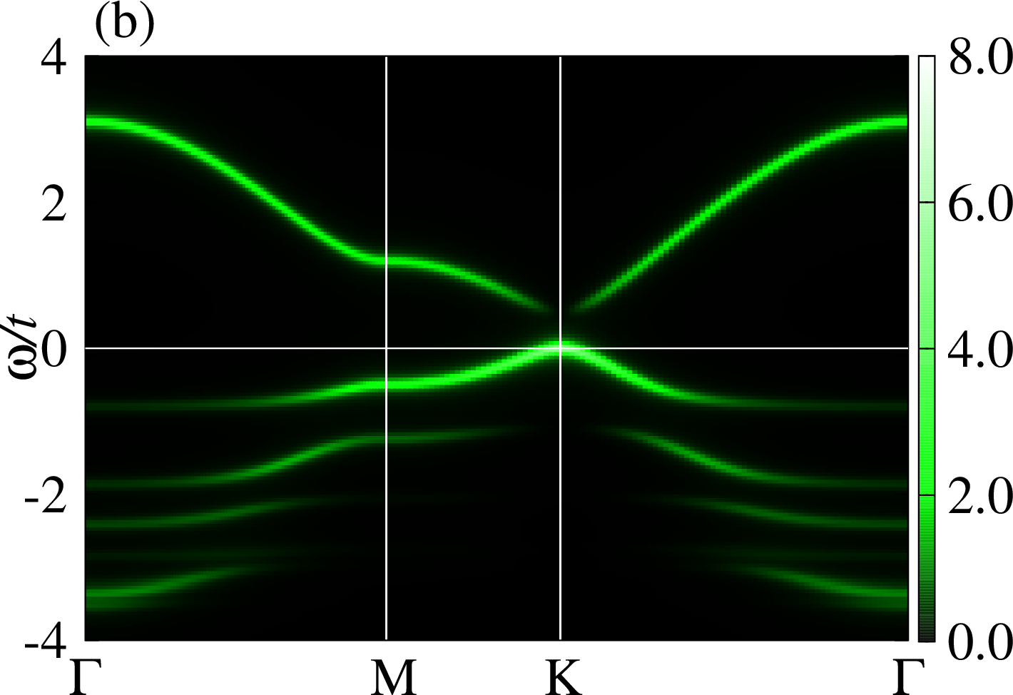
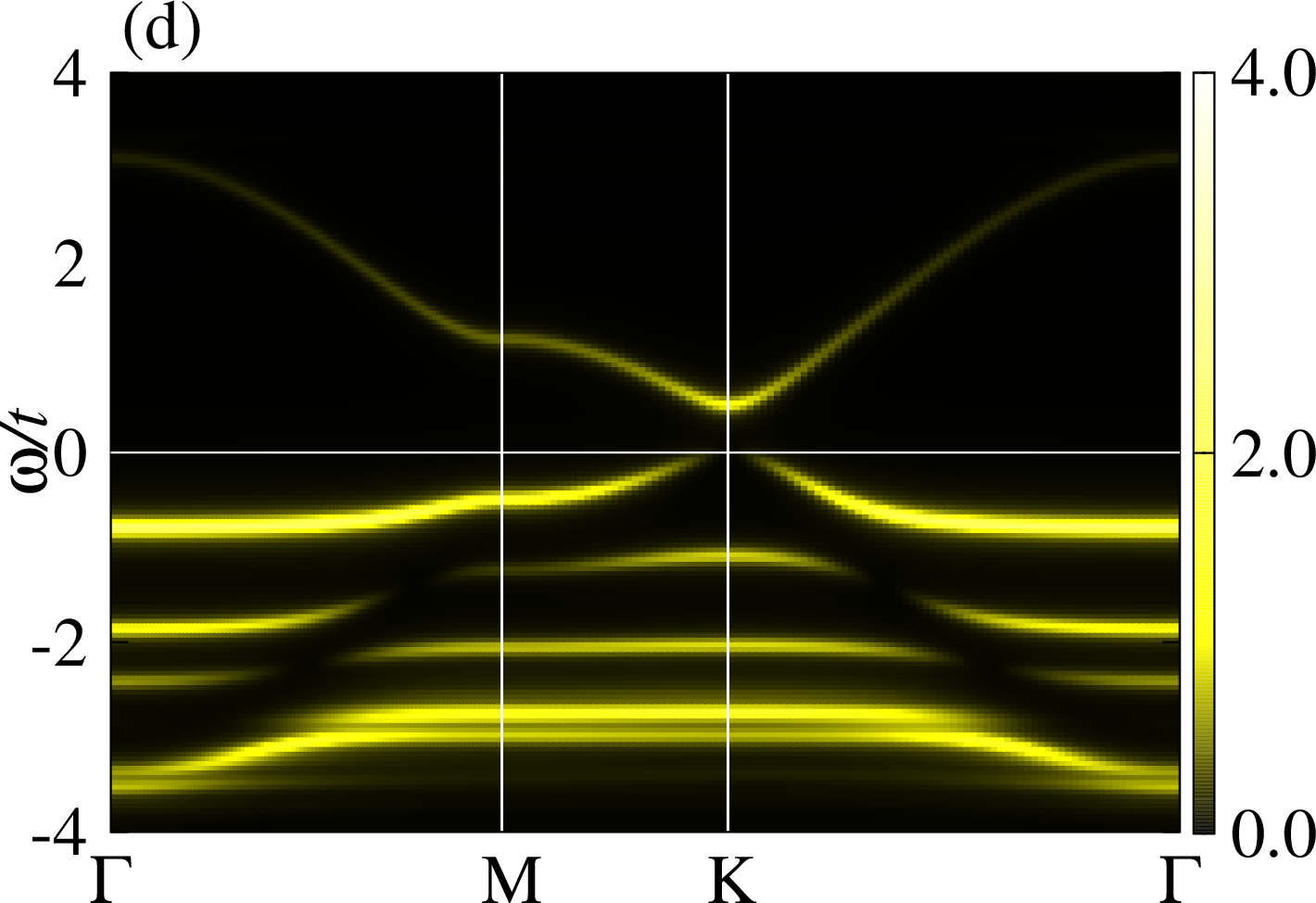
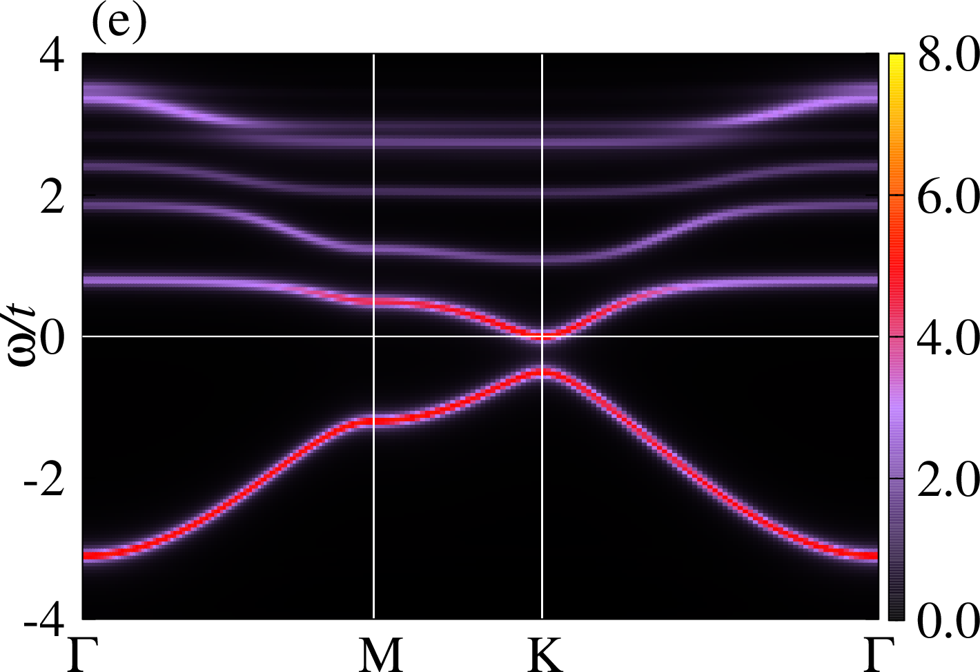
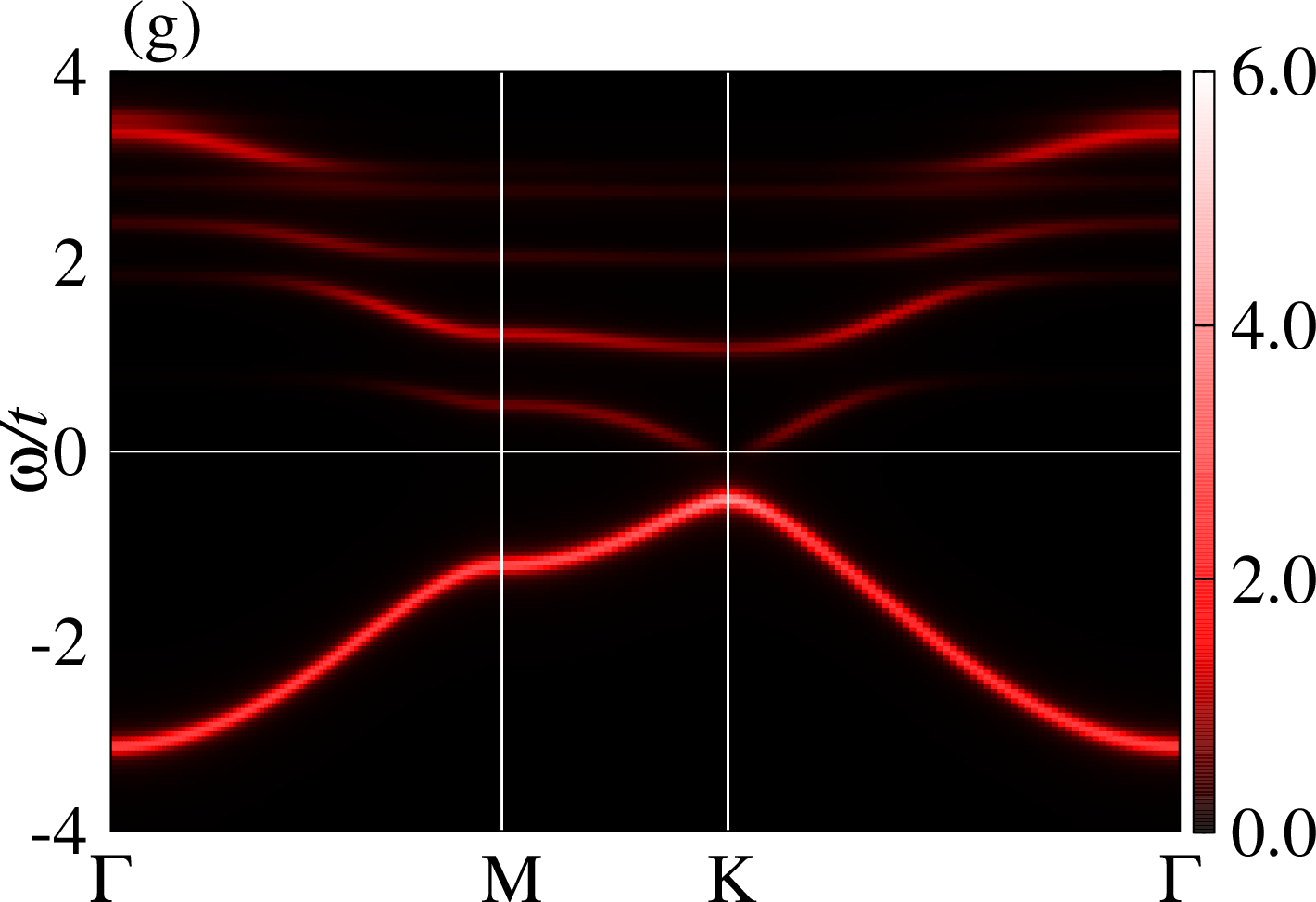
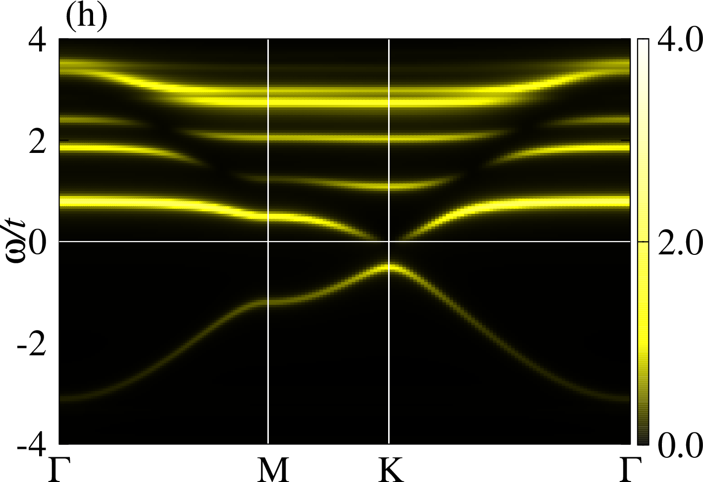
Figure 4: (color online) The CPT results of the single-particle excitation spectra for (a)–(d) up and (e)–(h) down electrons in the FM state at $T=0$. The calculations are for $U/t=4$ and $t_{sp}/t=1$ using the 9-site cluster (containing 3 unit cells). (a) and (e): $A_{\sigma}(\mathbf{k},\omega)=\sum_{\alpha}A_{\sigma}^{\alpha\alpha}(\mathbf{k},\omega)$, (b) and (f): $A^{AA}_{\sigma}(\mathbf{k},\omega)$, (c) and (g): $A^{BB}_{\sigma}(\mathbf{k},\omega)$, and (d) and (h): $A^{HH}_{\sigma}(\mathbf{k},\omega)$. A Lorentzian broadening of $\eta/t=0.05$ is used. The spectral intensity is indicated by a color bar in each figure. Notice that the different intensity scales are used for different figures. The Fermi energy $E_{\rm F}$ is located at $\omega=0$.

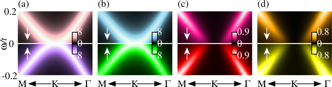
Figure 5: (color online) Same as Fig. 4 but the enlarged scale at the vicinity of $K$ point near the Fermi energy $E_{\rm F}$ (white lines). (a) $A_{\sigma}(\mathbf{k},\omega)=\sum_{\alpha}A_{\sigma}^{\alpha\alpha}(\mathbf{k},\omega)$, (b) $A^{AA}_{\sigma}(\mathbf{k},\omega)$, (c) $A^{BB}_{\sigma}(\mathbf{k},\omega)$, and (d) $A^{HH}_{\sigma}(\mathbf{k},\omega)$. Notice that the spectra $A^{\alpha\alpha}_{\uparrow}(\mathbf{k},\omega)$ and $A^{\alpha\alpha}_{\downarrow}(\mathbf{k},\omega)$ for up and down spins, respectively, are plotted with different colors below and above $E_{\rm F}$ at $\omega=0$. The region of momenta taken in the horizontal axis is $0.2\pi$ in the $K$-$M$ ($K$-$\Gamma$) direction from $K$.

It is also noticeable in Fig. 4 that (iii) the lowest single-particle excitations among the same spin have a finite gap $\Delta_{\rm c}$, suggesting that the spin conserved charge excitations are gapped, while (iv) the spin excitation gap should be zero since the lowest single-particle excitation gap $\Delta_{\rm s}$ among the opposite spins is zero, as shown in Fig. 5. We also examine the $U$ dependence of the single-particle excitation spectrum and find that (v) although $\Delta_{\rm c}$ ($\Delta_{\rm s}$) monotonically increases (remains zero) with increasing $U$, the effective mass $m^{*}$ simply deceases, where $m^{*}$ is inversely proportional to the curvature of the quadratic energy dispersion for the lowest single-particle excitations. As discussed in Sec. IV.1, these features (i)–(v) can be understood within a simple mean-field theory.

III.2.2 PM state

In sharp contrast to the results for the FM state, we find that the PM state exhibits the linear energy dispersions near $E_{\rm F}$. As shown in Fig. 6 for $U/t=4$, we can clearly observe that the massless Dirac quasiparticle excitations emerge with the Dirac point exactly at $E_{\rm F}$. The $U$ dependence of the single-particle excitations for the PM state is summarized in Fig. 7. The massless Dirac quasiparticle excitations always exist in the PM state as long as $U$ is finite. It is also interesting to notice in Fig. 7 that the Dirac Fermi velocity $v_{\rm F}$, i.e., the slope of the linear energy dispersion at $E_{\rm F}$, monotonically increases with increasing $U$ and approaches to the Dirac Fermi velocity $v_{0}=\sqrt{3}t/2$ of the pure graphene model in the limit of $U/t\to\infty$ (see also Fig. 8).

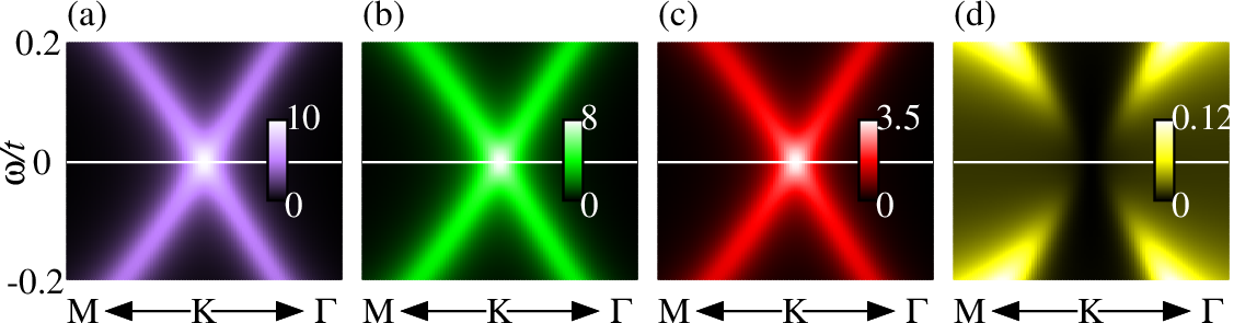
Figure 6: (color online) The CPT results of the single-particle excitation spectra in the PM state for $U/t=4$ and $t_{sp}/t=1$ obtained using the 9-site cluster (containing 3 unit cells) at $T/t=0.025$ around $K$ point near the Fermi energy $E_{\rm F}$ (white lines). (a) $A_{\sigma}(\mathbf{k},\omega)=\sum_{\alpha}A_{\sigma}^{\alpha\alpha}(\mathbf{k},\omega)$, (b) $A^{AA}_{\sigma}(\mathbf{k},\omega)$, (c) $A^{BB}_{\sigma}(\mathbf{k},\omega)$, and (d) $A^{HH}_{\sigma}(\mathbf{k},\omega)$. Here, we only show the spectra $A^{\alpha\alpha}_{\uparrow}(\mathbf{k},\omega)$ for up electrons, which are exactly the same as $A^{\alpha\alpha}_{\downarrow}(\mathbf{k},\omega)$. A Lorentzian broadening of $\eta/t=0.05$ is used. The spectral intensity is indicated by a color bar in each figure. Notice that the different intensity scales are used for different figures. The region of momenta taken in the horizontal axis is $0.2\pi$ in the $K$-$M$ ($K$-$\Gamma$) direction from $K$.

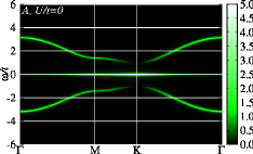
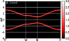
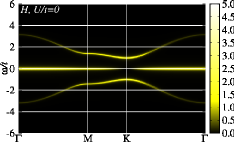
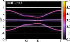
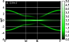
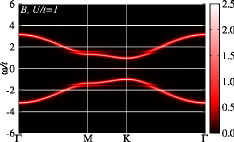
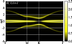
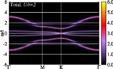
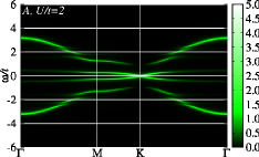
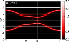
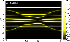
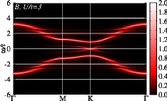
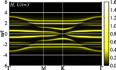
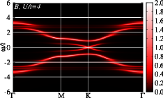
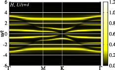
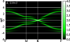
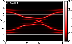
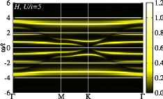
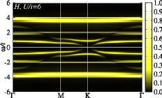
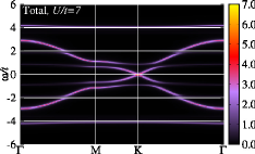
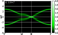
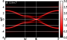
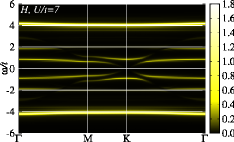
Figure 7: (color online) The CPT results of the single-particle excitation spectra for $U/t=0,1,\cdots,7$ (from top to bottom panels) and $t_{sp}/t=1$ in the PM state at $T=0$ obtained using 9-site cluster (containing 3 unit cells). $A_{\sigma}(\mathbf{k},\omega)=\sum_{\alpha}A^{\alpha\alpha}_{\sigma}(\mathbf{k},\omega)$, $A^{AA}_{\sigma}(\mathbf{k},\omega)$, $A^{BB}_{\sigma}(\mathbf{k},\omega)$, and $A^{HH}_{\sigma}(\mathbf{k},\omega)$ are shown from left to right panels. Here, we only show the spectra for up electrons, which are exactly the same as $A^{\alpha\alpha}_{\downarrow}(\mathbf{k},\omega)$. A Lorentzian broadening of $\eta/t=0.05$ is used. The spectral intensity is indicated by a color bar in each figure. Note that the different intensity scales are used for different figures. The Fermi energy $E_{\rm F}$ is located at $\omega=0$.

While the simplest mean-field theory and the DFT calculations can reproduce qualitatively the FM state with the quadratic energy dispersion, they fail to capture the Dirac-like quasiparticle excitations with the linear energy dispersion in the PM state Zhou2009 . The inability of describing the massless Dirac quasiparticles in the single-particle approximations immediately implies that the dynamical correlation effect is responsible for the emergent massless Dirac quasiparticles, which will be discussed more.

We should also notice in Fig. 6 and Fig. 7 that the emergent massless Dirac quasiparticles are composed of $A$ and $B$ orbitals, but not $H$ orbital: while the contribution of $A$ ($H$) orbital to the low energy spectral weight near $K$ point (and also $K^{\prime}$ point) remains large (vanishing) with varying $U$, the contribution of $B$ orbital is small but finite for small $U$ and gradually increases as the massless Dirac quasiparticles becomes more visible in the single-particle excitation spectrum for large $U$.

To be more quantitative, we also evaluate the spectral weight for $\alpha$ orbital at the Dirac point with $\omega=0$,

$$\rho^{\alpha\alpha}_{K}:=-\lim_{\eta\rightarrow 0^{+}}\frac{\eta}{\pi}\Im{\cal G}^{\alpha\alpha}_{\sigma}(\mathbf{k}=K,i\eta),$$ (11)

where $0^{+}$ is positive infinitesimal, and find that $\rho^{AA}_{K}=1$ and $\rho^{HH}_{K}=0$ (the same also at $K^{\prime}$ point), irrespectively of the value of $U$, whereas $\rho^{BB}_{K}$ increases monotonically from zero with increasing $U$, as shown in Fig. 8. This is understood by recalling that in the noninteracting limit, $A$ orbital is completely decoupled from $H$ orbital at $K$ and $K^{\prime}$ points where $\gamma_{\mathbf{k}}=0$ [see Eq. (3)]. Therefore, even when the interaction $U$ on the hydrogen impurity sites is turned on, the contribution from $A$ orbital to the spectral weight at $K$ and $K^{\prime}$ points remains the same.

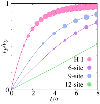
Figure 8: (color online) $U$ dependence of the Dirac Fermi velocity $v_{\rm F}$ calculated using the CPT and the Hubbard-I (H-I) approximation. The CPT calculations are done for the 6-site cluster (containing 2 unit cells) at $T=0.025t$ in the PM phase, and for the 9-site cluster (containing 3 unit cells) and the 12-site cluster (containing 4 unit cells) at $T=0$ where the PM state is assumed. Both calculations are for $t_{sp}/t=1$ at $n=1$. The size of dots is proportional to the spectral weight $\rho_{K}^{BB}$ for $B$ orbital at the Fermi energy and $v_{0}=\sqrt{3}t/2$ is the Dirac Fermi velocity of the pure graphene model.

We also examine the finite size effects on the single-particle excitations in the PM state using three different clusters and find no qualitative difference. Namely, as shown in Fig. 9, we still find the emergent massless Dirac quasiparticles at $K$ and $K^{\prime}$ points with the Dirac points exactly at $E_{\rm F}$ and the same characteristic features of their spectral weights. Although the emergent massless Dirac quasiparticles are not clear for the 12-site calculations shown in the bottom panels of Fig. 9, it is indeed apparent in the enlarged scale near $E_{\rm F}$ shown in Fig. 10. Therefore, the emergence of the massless Dirac quasiparticles is not subjected to the finite size effects of the clusters.

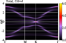
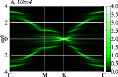
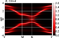
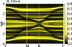
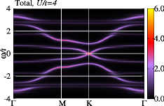
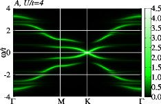
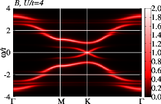
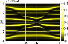
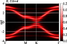
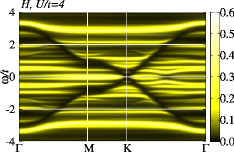
Figure 9: (color online) The CPT results of the single-particle excitation spectra in the PM state for $U/t=4$ and $t_{sp}/t=1$ obtained using the 6-site cluster (containing 2 unit cells) at $T=0.025t$, the 9-site cluster (containing 3 unit cells) at $T=0$, and the 12-site cluster (containing 4 unit cells) at $T=0$ (from top to bottom panels). $A_{\sigma}(\mathbf{k},\omega)=\sum_{\alpha}A^{\alpha\alpha}_{\sigma}(\mathbf{k},\omega)$, $A^{AA}_{\sigma}(\mathbf{k},\omega)$, $A^{BB}_{\sigma}(\mathbf{k},\omega)$, and $A^{HH}_{\sigma}(\mathbf{k},\omega)$ are shown from left to right panels. A Lorentzian broadening of $\eta/t=0.05$ is used. The spectral intensity is indicated by a color bar in each figure. Note that the different intensity scales are used for different figures. The Fermi energy $E_{\rm F}$ is located at $\omega=0$. Although the emergent massless Dirac quasiparticles for the 12-site calculations (bottom panels) are not as clear as the other cases, it becomes apparent in the enlarged scale near $E_{\rm F}$, as shown in Fig. 10.

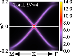
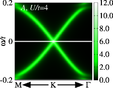
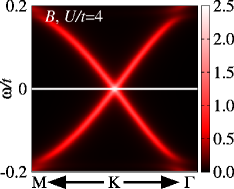
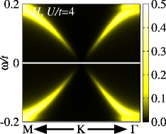
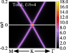
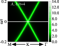
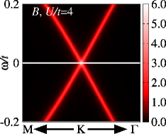
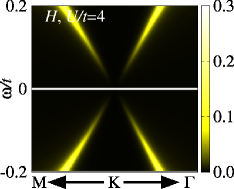
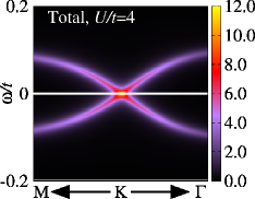
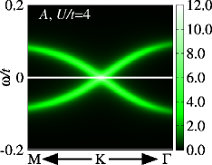
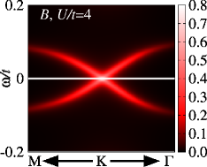
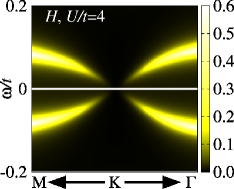
Figure 10: (color online) Same as Fig. 9 but the enlarged scale at the vicinity of $K$ point near the Fermi energy $E_{\rm F}$ (white lines). A Lorentzian broadening of $\eta/t=0.01$ is used. The region of momenta taken in the horizontal axis is $0.2\pi$ in the $K$-$M$ ($K$-$\Gamma$) direction from $K$.

On the other hand, we find in Fig. 9 and Fig. 10 that the Dirac Fermi velocity $v_{\rm F}$ depends quantitatively on the cluster size used. The $U$ dependence of $v_{\rm F}$ for three different clusters is summarized in Fig. 8. Although the value itself depends on the cluster size, the qualitative behavior of $v_{\rm F}$ is the same: $v_{\rm F}$ monotonically increases with increasing $U$ for all clusters used. It is also interesting to note that, irrespectively of the cluster sizes, the spectral weight $\rho^{BB}_{K}$ for $B$ orbital at the Dirac point is found to be proportional to $v_{\rm F}^{2}$, i.e.,

$$\rho^{BB}_{K}=\left(\frac{v_{\rm F}}{v_{0}}\right)^{2},$$ (12)

as shown in Fig. 11. This universal behavior is intuitively understood by assuming that the electron annihilation operator is renormalized with the renormalization factor $z_{A}$ ($z_{B}$) for $A$ ($B$) orbital at the Dirac point $k_{\rm F}$, i.e., $c_{k_{\rm F}\sigma A(B)}\to z_{A(B)}c_{k_{\rm F}\sigma A(B)}$ with $z_{A}\approx 1$. Due to this renormalization, $\rho^{BB}_{K}\sim z_{B}^{2}$ while $v_{\rm F}/v_{0}\sim z_{B}$ because $t$ is renormalized to $tz_{A}z_{B}$. The simple and yet significant universal relation in Eq. (12) concisely expresses the inevitable involvement of $B$ orbital in the low-energy excitations for the emergent massless Dirac quasiparticles.

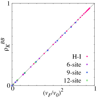
Figure 11: (color online) The spectral weight $\rho_{K}^{BB}$ for $B$ orbital at the Fermi energy $E_{\rm F}$ and momentum ${\mathbf{k}}=K$ versus $v_{\rm F}^{2}$ calculated using the CPT and the Hubbard-I (H-I) approximation. The CPT calculations are done for the 6-site cluster (containing 2 unit cells) at $T=0.025t$ in the PM phase, and for the 9-site cluster (containing 3 unit cells) and the 12-site cluster (containing 4 unit cells) at $T=0$ where the PM state is assumed. Both calculations are for $t_{sp}/t=1$ at $n=1$ with various values of $U$ shown in Fig. 8. Here, $v_{0}=\sqrt{3}t/2$ is the Dirac Fermi velocity of the pure graphene model.

Finally, we summarize how the massless Dirac quasiparticles emerge and evolve with increasing $U$ and how different orbitals contribute to the formation of the massless Dirac quasiparticles. As shown in Fig. 7, the spectral weight $A^{BB}_{\sigma}(\mathbf{k},\omega)$ for $B$ orbital around the Fermi energy is exactly zero when $U=0$ since $B$ orbital does not contribute to the flat band formation in the noninteracting limit (see also Fig. 2). However, with increasing $U$, $A^{BB}_{\sigma}(\mathbf{k},\omega)$ around $K$ and $K^{\prime}$ points near the Fermi energy gradually increases to form the massless Dirac quasiparticles. On the other hand, the $A$ orbital component of the spectral weight $A^{AA}_{\sigma}(\mathbf{k},\omega)$ at the Fermi energy is already finite even when $U=0$, since $A$ orbital contributes to the formation of the flat band in the noninteracting limit, and as $U$ increases it develops into the low energy excitations with the linear energy dispersions at $K$ and $K^{\prime}$ points. As shown in Sec. IV.2, these features are in good agreement with those obtained in the Hubbard-I approximation.

The contribution of $H$ orbital is different. First, we notice in Fig. 7 that the spectral weight $A^{HH}_{\sigma}(\mathbf{k},\omega)$ for $H$ orbital displays almost dispersionless spectra, indicating that $H$ orbital is rather localized in real space, even when $U$ is small. Furthermore, as clearly observed in Fig. 7 and Fig. 9, $A^{HH}_{\sigma}(\mathbf{k},\omega)$ exhibits a “dark spectral” region where no spectral intensity exists and the “dispersion” of the dark spectral region very much resembles the energy dispersion of the conduction band described by the pure graphene model, i.e., $\omega=\pm|\gamma_{\mathbf{k}}|$, suggesting that

$$A^{HH}_{\sigma}(\mathbf{k},\omega=\pm|\gamma_{\mathbf{k}}|)=0.$$ (13)

This is exactly the case for the Hubbard-I approximation, as discussed in Sec. IV.2, because $G_{\sigma}^{HH}(\mathbf{k},\omega=\pm|\gamma_{\mathbf{k}}|)=0$ in Eq. (34) (see also Fig. 16). This implies that $H$ orbital is “level repulsive”, i.e., dynamically decoupled to the conduction band composed of $A$ and $B$ orbitals, and thus $H$ orbital does not contribute to the formation of the emergent massless Dirac quasiparticles.

IV Analytical results

In this section, the periodic Anderson model is analyzed using the simplest mean-filed theory for the FM state and the Hubbard-I approximation for the PM state. We also construct an effective Hamiltonian to describe the single-particle excitations in the PM state and discuss the chiral symmetry of the quasiparticles as well as the origin of the emergent massless Dirac quasiparticles.

IV.1 Mean-field approximation

We first consider the simplest mean-field theory for the FM state to show that the main characteristic features of the single-particle excitations obtained by the CPT in Sec. III.2.1 can be reproduced by the single-particle approximation. Applying the mean-field decoupling to the on-site Coulomb term for the hydrogen impurity sites,

$$n_{\mathbf{r}_{i}\uparrow H}n_{\mathbf{r}_{i}\downarrow H} \approx n_{\mathbf{r}_{i}\uparrow H}\left<n_{\mathbf{r}_{i}\downarrow H}\right>+n_{\mathbf{r}_{i}\downarrow H}\left<n_{\mathbf{r}_{i}\uparrow H}\right>$$ (14)

$$- \left<n_{\mathbf{r}_{i}\uparrow H}\right>\left<n_{\mathbf{r}_{i}\downarrow H}\right>,$$

the mean-field Hamiltonian $\mathcal{H}_{\rm MF}$ for the periodic Anderson model with $\epsilon_{H}=-U/2$ is given as

$$\mathcal{H}_{\rm MF} = \sum_{\bf k}\sum_{\sigma}\mathbf{c}^{\dagger}_{\mathbf{k}\sigma}\left(\begin{array}[]{ccc}0&\gamma_{\bf k}&0\\ \gamma_{\bf k}^{\ast}&0&t_{sp}\\ 0&t_{sp}&\Delta_{\bar{\sigma}}\\ \end{array}\right)\mathbf{c}_{\mathbf{k}\sigma}$$ (18)

$$- U\sum_{i}\left<n_{\mathbf{r}_{i}\uparrow H}\right>\left<n_{\mathbf{r}_{i}\downarrow H}\right>,$$ (19)

where

$$\Delta_{\sigma}=U\left(\left<n_{\mathbf{r}_{i}\sigma H}\right>-\frac{1}{2}\right)$$ (20)

and $\bar{\sigma}$ denotes the opposite spin of $\sigma$. We assume that $\left<n_{\mathbf{r}_{i}\sigma H}\right>$ is site independent.

Assuming the FM ansatz, i.e.,

$$\Delta_{\uparrow}=-\Delta_{\downarrow}=\Delta,$$ (21)

we can easily obtain the single-particle excitation spectrum of ${\mathcal{H}}_{\rm MF}$ for a given $\Delta$. A typical example of the single-particle excitation spectrum for the FM state is shown in Fig. 12. The main features are summarized as follows. First, for any $t_{sp}$ and $\Delta>0$, the Fermi energy locates at the top (bottom) of the middle band for up (down) electrons, thus indicating that the total magnetic moment $2S$ is exactly $|H|+|A|-|B|$, independently of the value of $\Delta\,(>0)$. Second, the top of the middle band for up electrons and the bottom of the middle band for down electrons touch exactly at the Fermi energy and momentum ${\bf k}=K$ and $K^{\prime}$. This degeneracy is easily understood because $\gamma_{\bf k}=0$ at $K$ and $K^{\prime}$ points, and therefore one of the eigenvalues of $3\times 3$ matrices in Eq. (19) for each spin component must be zero at these momenta. This also indicates that the energy dispersion is quadratic near the Fermi energy. It should be also noticed in Fig. 12 that the low-energy excitations close to the Fermi energy is mostly composed of $A$ orbital and indeed only $A$ orbital contributes to the spectral weight at the Fermi energy. These results are qualitatively the same as those obtained using the CPT in Fig. 4 and Fig. 5.

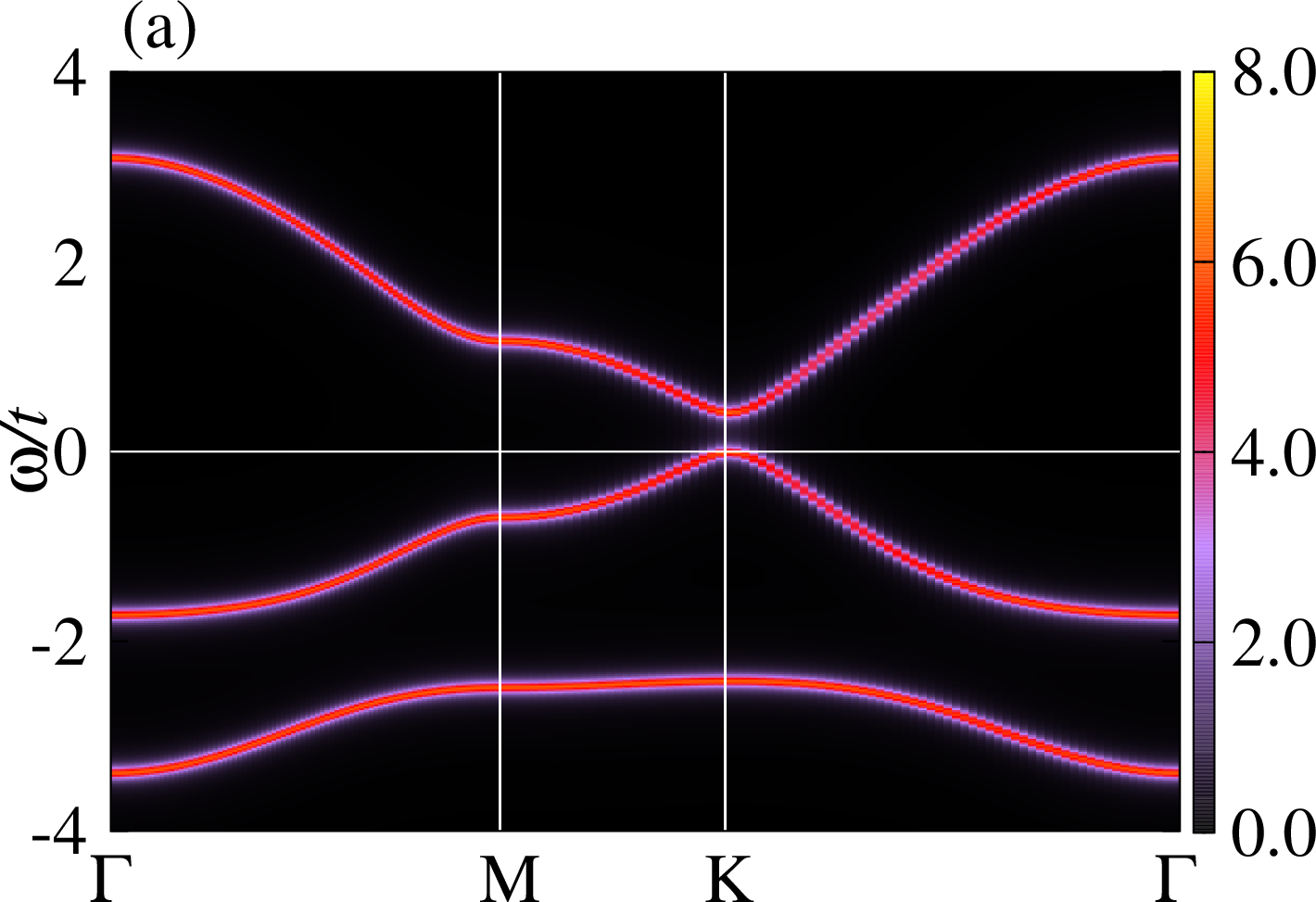
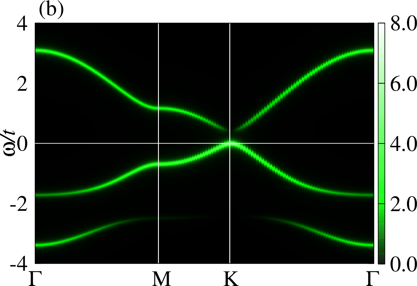
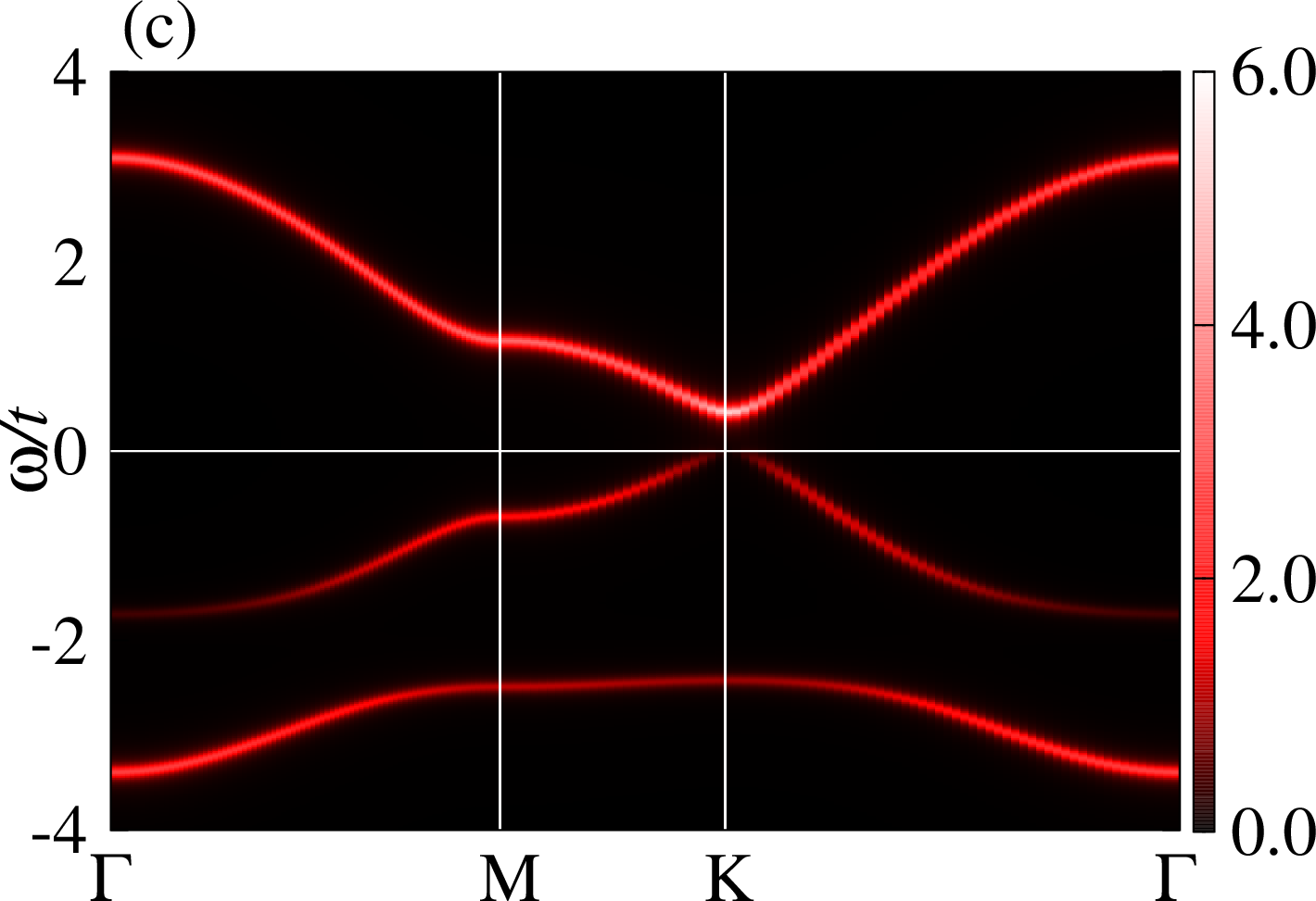
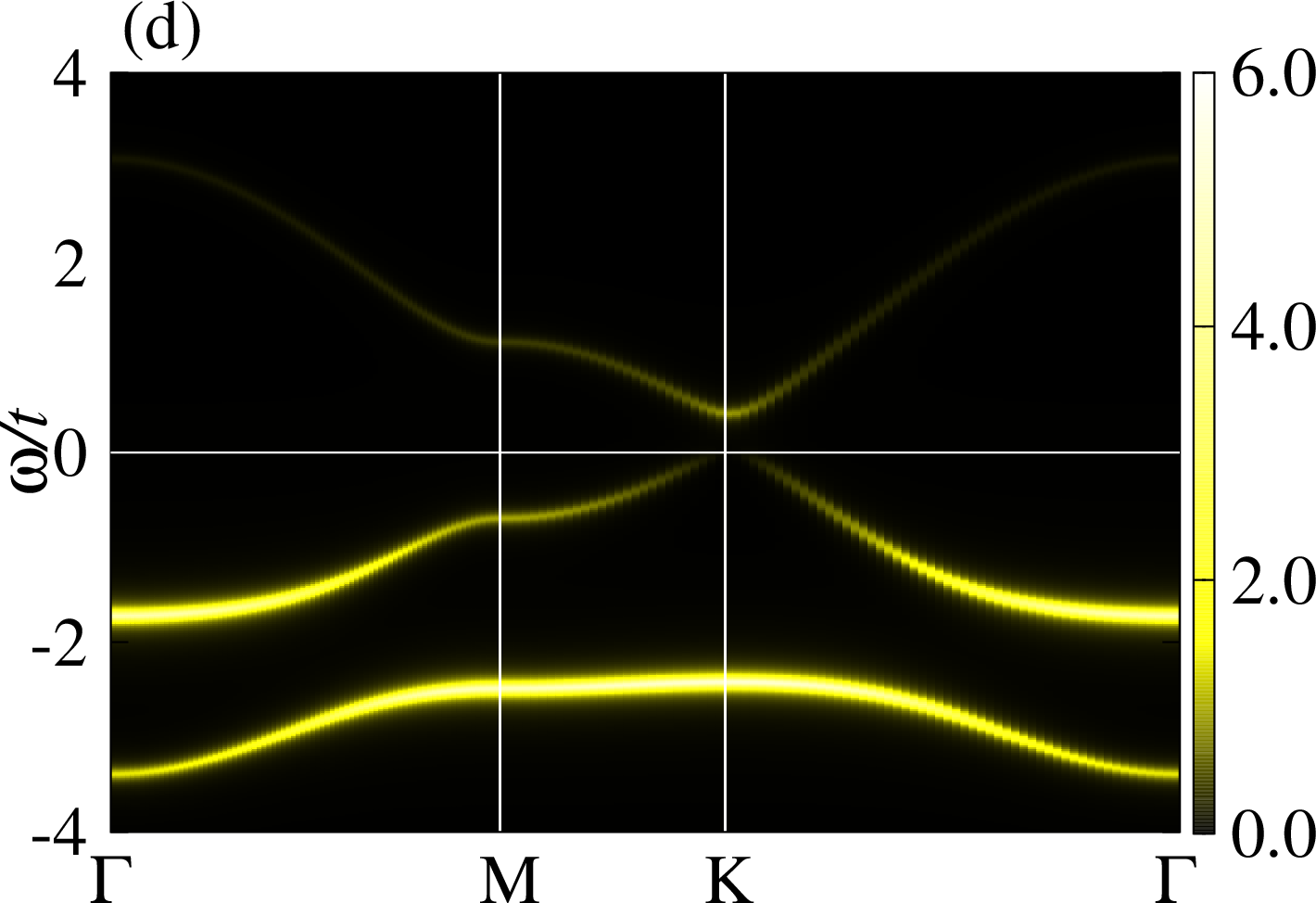
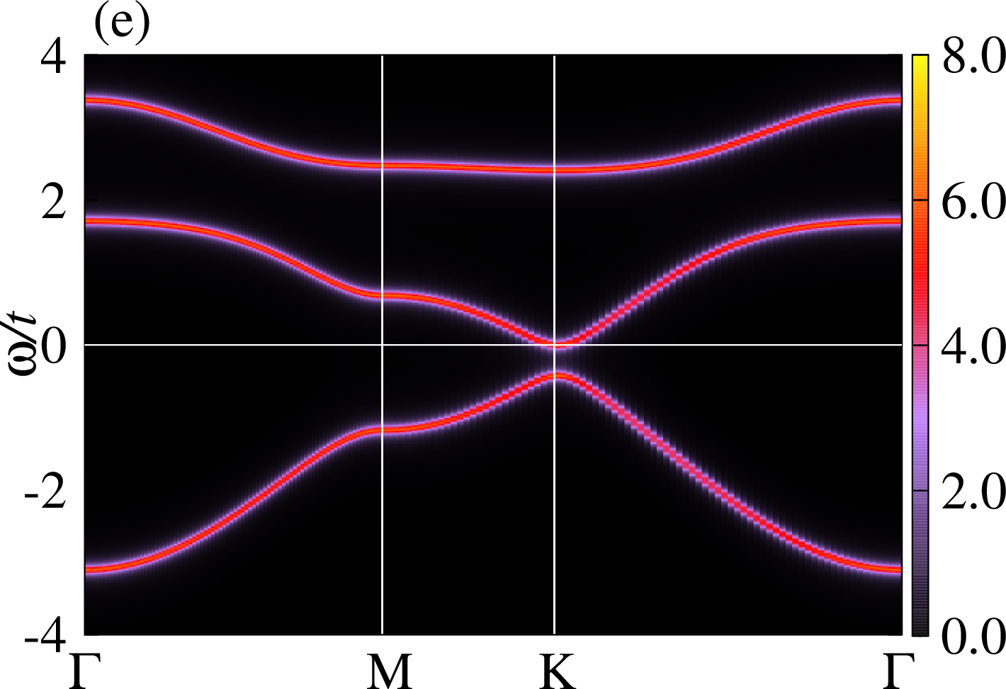
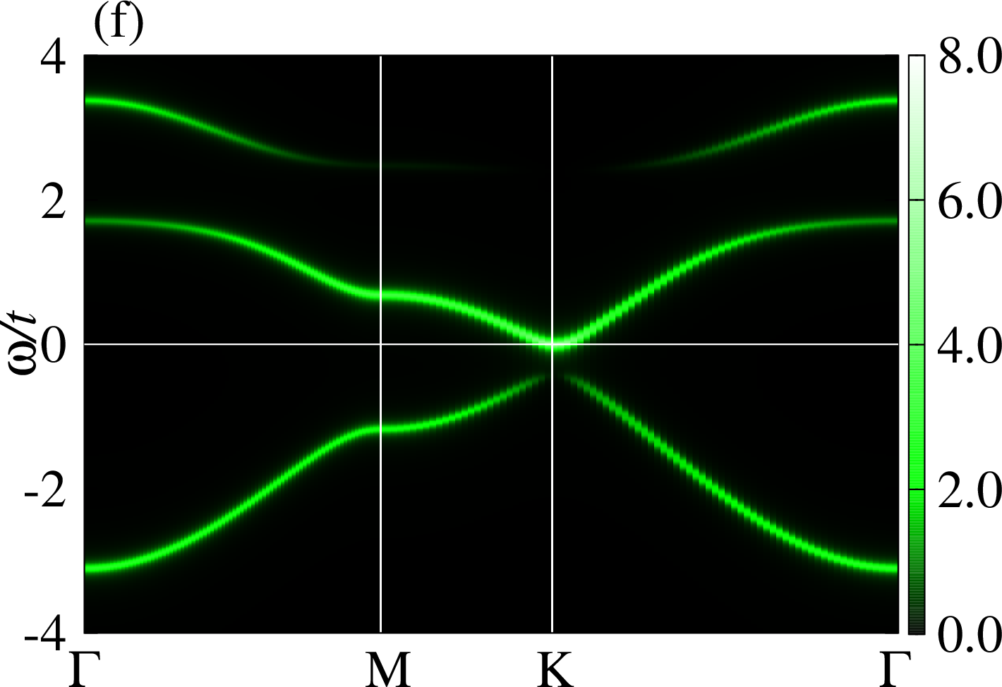
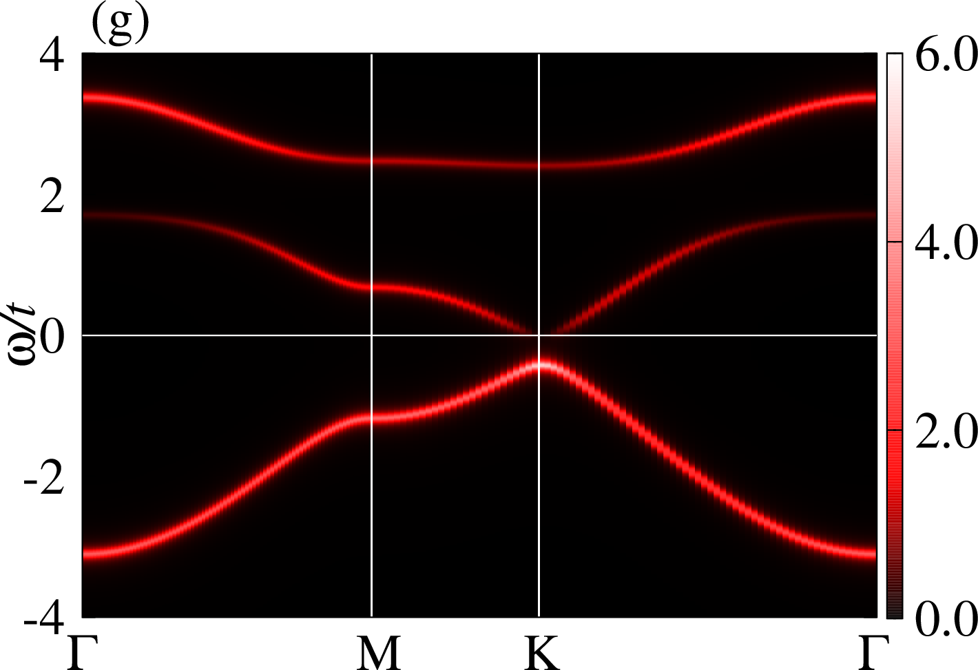
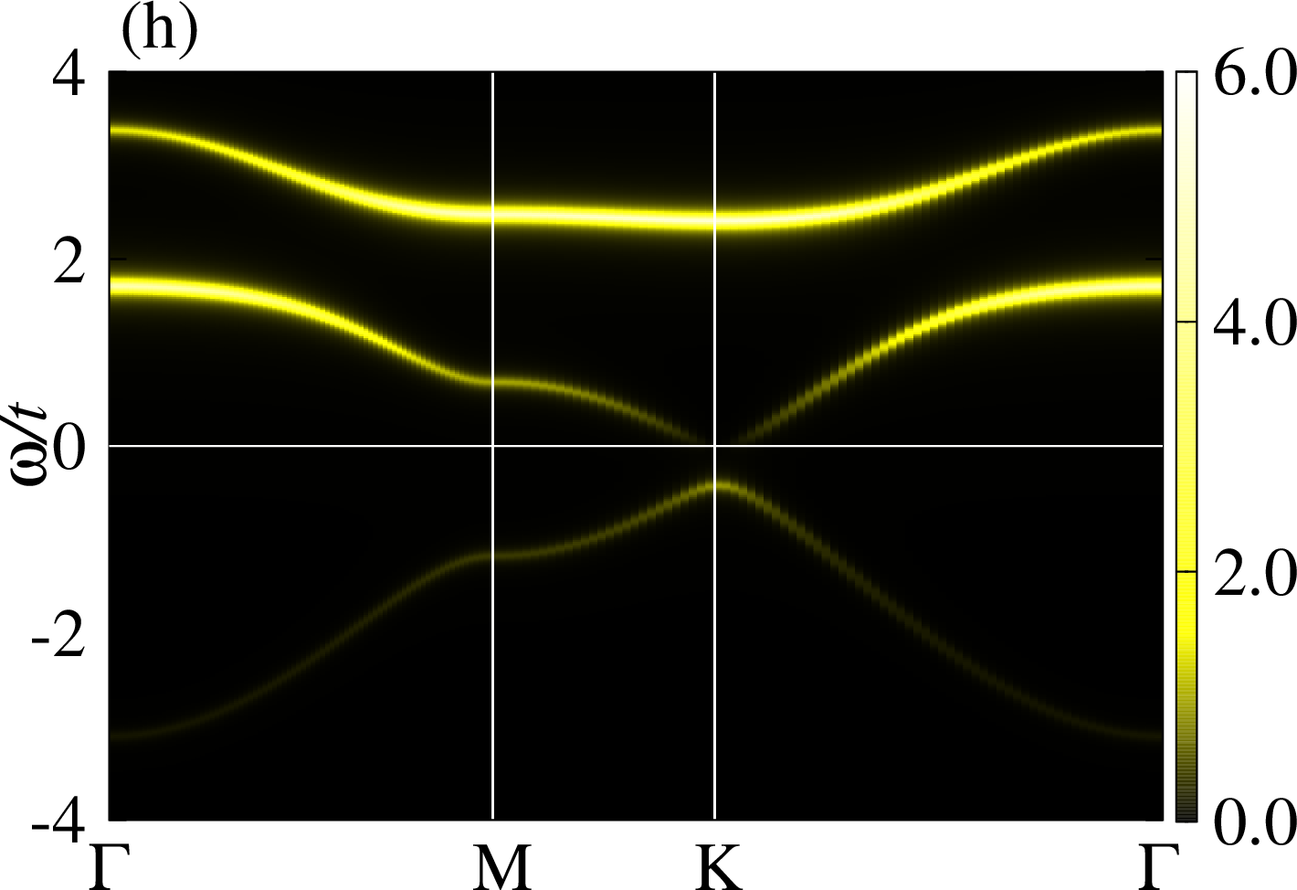
Figure 12: (color online) The mean-field results of the single-particle excitation spectra for (a)–(d) up and (e)–(h) down electrons in the FM state at $T=0$. The calculations are for $t_{sp}/t=1$ and $\Delta/t=2$ at $n=1$. (a) and (e): $A_{\sigma}(\mathbf{k},\omega)=\sum_{\alpha}A_{\sigma}^{\alpha\alpha}(\mathbf{k},\omega)$, (b) and (f): $A^{AA}_{\sigma}(\mathbf{k},\omega)$, (c) and (g): $A^{BB}_{\sigma}(\mathbf{k},\omega)$, and (d) and (h): $A^{HH}_{\sigma}(\mathbf{k},\omega)$. A Lorentzian broadening of $\eta/t=0.05$ is used. The spectral intensity is indicated by a color bar in each figure. Notice that the different intensity scales are used for different figures. The Fermi energy $E_{\rm F}$ is located at $\omega=0$.

IV.2 Hubbard-I approximation

It is highly interesting to examine the single-particle excitations in the PM state using the Hubbard-I approximation Hubbard1963 since this is the simplest approximation to treat dynamical electron correlations with no spatial fluctuations.

IV.2.1 Self-energy

Within the Hubbard-I approximation Hubbard1963 , the self-energy $\Sigma_{\sigma}(\omega)$ of the single-particle Green’s function for the hydrogen impurity site with spin $\sigma$ is given as

$$\Sigma_{\sigma}(\omega)=U\langle n_{\mathbf{r}_{i}\bar{\sigma}H}\rangle+U^{2}\frac{\langle n_{\mathbf{r}_{i}\bar{\sigma}H}\rangle\left(1-\langle n_{\mathbf{r}_{i}\bar{\sigma}H}\rangle\right)}{\omega-\epsilon_{H}-U\left(1-\langle n_{\mathbf{r}_{i}\bar{\sigma}H}\rangle\right)}.$$ (22)

Assuming the PM state at half-filling, i.e., $\langle n_{\mathbf{r}_{i}\uparrow H}\rangle=\langle n_{\mathbf{r}_{i}\downarrow H}\rangle=1/2$ and $\epsilon_{H}=-U/2$, the self-energy is

$$\Sigma_{\sigma}(\omega)=\frac{U}{2}+\frac{U^{2}}{4\omega}.$$ (23)

IV.2.2 Dispersion relation

Once the self energy $\Sigma_{\sigma}(\omega)$ is obtained, the inverse of the interacting single-particle Green’s function $\boldsymbol{G}_{\sigma}(\mathbf{k},\omega)$ for spin $\sigma$ and momentum $\mathbf{k}$ is simply given as

$$\boldsymbol{G}_{\sigma}^{-1}(\mathbf{k},\omega) = \boldsymbol{G}^{-1}_{0\sigma}(\mathbf{k},\omega)-\boldsymbol{\Sigma}_{\sigma}(\omega)$$ (27)

$$= \left(\begin{array}[]{ccc}\omega&-\gamma_{\mathbf{k}}&0\\ -\gamma^{*}_{\mathbf{k}}&\omega&-t_{sp}\\ 0&-t_{sp}&\omega-\epsilon_{H}-\Sigma_{\sigma}(\omega)\end{array}\right),$$

where $\boldsymbol{G}_{0\sigma}(\mathbf{k},\omega)$ is the noninteracting single-particle Green’s function. In this matrix representation, the bases for the first, second, and third column and row correspond to $A$, $B$, and $H$ orbitals, respectively. The particle-hole symmetry is guaranteed by setting the on-site energy of the hydrogen impurity site to be $\epsilon_{H}=-\frac{U}{2}$. The dispersion relation of the single-particle excitations is obtained as the poles of the single-particle Green’s function. Thus, by solving the following equation

$$\det\boldsymbol{G}_{\sigma}^{-1}(\omega,\mathbf{k}) = \frac{1}{\omega}\left\{\omega^{4}-\left(\frac{U^{2}}{4}+|\gamma_{\mathbf{k}}|^{2}+t_{sp}^{2}\right)\omega^{2}\right.$$ (28)

$$\quad\quad\quad+\left.\frac{U^{2}}{4}|\gamma_{\mathbf{k}}|^{2}\right\}=0,$$

we find that there exist four poles at $\omega_{1,{\mathbf{k}}}=\omega_{+,{\mathbf{k}}}$, $\omega_{2,{\mathbf{k}}}=\omega_{-,{\mathbf{k}}}$, $\omega_{3,{\mathbf{k}}}=-\omega_{-,{\mathbf{k}}}$, and $\omega_{4,{\mathbf{k}}}=-\omega_{+,{\mathbf{k}}}$, where

$$\omega_{\pm,\mathbf{k}}^{2}=\frac{1}{2}\left\{\left(\frac{U^{2}}{4}+|\gamma_{\mathbf{k}}|^{2}+t_{sp}^{2}\right)\pm\sqrt{\left(\frac{U^{2}}{4}+|\gamma_{\mathbf{k}}|^{2}+t_{sp}^{2}+U|\gamma_{\mathbf{k}}|\right)\left(\frac{U^{2}}{4}+|\gamma_{\mathbf{k}}|^{2}+t_{sp}^{2}-U|\gamma_{\mathbf{k}}|\right)}\right\}$$ (29)

and $\omega_{\pm,\mathbf{k}}\geq 0$, i.e., $\omega_{1,\mathbf{k}}\geq\omega_{2,\mathbf{k}}\geq 0\geq\omega_{3,\mathbf{k}}\geq\omega_{4,\mathbf{k}}$. The dispersion relation for various $U$ is shown in Fig. 13. It is interesting to notice in Fig. 13 that the inner two bands with $\nu=2$ and $3$ exhibit the massless Dirac dispersions at $K$ and $K^{\prime}$ points with the Dirac points exactly at the Fermi energy as soon as a finite $U$ is turned on, thus in good qualitative agreement with the results obtained by the CPT in Sec. III.2.2. It should be also noted that the outer two bands with $\nu=1$ and $4$ shown in Fig. 13 correspond to the upper and lower Hubbard bands, respectively.

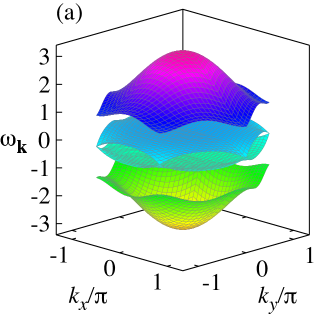
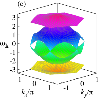
Figure 13: (color online) Single-particle excitation dispersion $\omega_{\mathbf{k}}$ (in unit of $t$) for $U/t=1$ (a), $3$ (b), and $5$ (c) with $t_{sp}/t=1$ obtained by the Hubbard-I approximation. Note that the inner (outer) two bands correspond to $\omega_{\mathbf{k}}=\pm\omega_{-,\mathbf{k}}$ ($\pm\omega_{+,\mathbf{k}}$). The Fermi energy $E_{\rm F}$ is located at $\omega_{\mathbf{k}}=0$. The inner two bands display the massless Dirac dispersions at $K$ and $K^{\prime}$ points with the Dirac points exactly at $E_{\rm F}$, and the outer two bands correspond to the upper and lower Hubbard bands.

IV.2.3 Dirac Fermi velocity

Let us define $\boldsymbol{\kappa}=\mathbf{k}-{\mathbf{k}}_{K}$ ($\boldsymbol{\kappa}=\mathbf{k}-{\mathbf{k}}_{K^{\prime}}$) and $\kappa=|\boldsymbol{\kappa}|$, where $\mathbf{k}_{K}$ ($\mathbf{k}_{K^{\prime}}$) is the momentum at $K$ ($K^{\prime}$) point. By expanding $|\gamma_{\mathbf{k}}|\simeq v_{0}\kappa\ll 1$ around $K$ ($K^{\prime}$) point, we obtain the massless Dirac quasiparticle dispersion

$$\pm\omega_{-,\mathbf{k}}\simeq\pm v_{\rm F}\kappa,$$ (30)

where $v_{\rm F}$ is the Dirac Fermi velocity

$$v_{\rm F}=\frac{U}{\sqrt{U^{2}+4t_{sp}^{2}}}v_{0}.$$ (31)

Here, $v_{0}=\sqrt{3}t/2$ is the Dirac Fermi velocity of the pure graphene model.

In the small $U$ limit (i.e., $U\ll|t_{sp}|$), the Dirac Fermi velocity increases linearly with $U$,

$$v_{\rm F}\simeq\frac{U}{2|t_{sp}|}v_{0},$$ (32)

while in the large $U$ limit (i.e., $U\gg|t_{sp}|$), the Dirac Fermi velocity is approximated as

$$v_{\rm F}\simeq\frac{U}{U+J_{\mathrm{K}}/4}v_{0},$$ (33)

where $J_{\mathrm{K}}=8t_{sp}^{2}/U$ is the Kondo coupling between a localized spin on the hydrogen impurity site and a conduction electron on the carbon site [see Eq. (85)]. As shown in Fig. 8, we find that $v_{\rm F}$ monotonically increases from zero with increasing $U$ and reaches to $v_{0}$ in the limit of $U/t\to\infty$. Therefore, $v_{\rm F}$ calculated by the Hubbard-I approximation is qualitatively compared with the result obtained by the CPT.

IV.2.4 Spectral representation

Simply inverting the $3\times 3$ matrix in Eq. (27), we can obtain the single-particle Green’s function

$$\boldsymbol{G}_{\sigma}(\mathbf{k},\omega)=\frac{1}{\det\boldsymbol{G}_{\sigma}^{-1}(\mathbf{k},\omega)}\\ \left(\begin{array}[]{ccc}\omega^{2}-\frac{1}{4}\left(U^{2}+4t_{sp}^{2}\right)&\gamma_{\mathbf{k}}\left(\omega-\frac{U^{2}}{4\omega}\right)&t_{sp}\gamma_{\mathbf{k}}\\ \gamma_{\mathbf{k}}^{*}\left(\omega-\frac{U^{2}}{4\omega}\right)&\omega^{2}-\frac{U^{2}}{4}&t_{sp}\omega\\ t_{sp}\gamma_{\mathbf{k}}^{*}&t_{sp}\omega&\omega^{2}-|\gamma_{\mathbf{k}}|^{2}\end{array}\right),$$ (34)

where the determinant is readily evaluated using Eqs. (28) and (29) as

$$\det\boldsymbol{G}_{\sigma}^{-1}(\mathbf{k},\omega)=\frac{1}{\omega}\prod_{\nu=1}^{4}(\omega-\omega_{\nu,\mathbf{k}}).$$ (35)

The spectral representation of the single-particle Green’s function is thus

$$\boldsymbol{G}_{\sigma}(\mathbf{k},\omega)=\sum_{\nu=1}^{4}\frac{\boldsymbol{\rho}_{\nu,\mathbf{k}}}{\omega-\omega_{\nu,\mathbf{k}}},$$ (36)

where $\boldsymbol{\rho}_{\nu,\mathbf{k}}$ is a $3\times 3$ matrix and its element $\left(\boldsymbol{\rho}_{\nu,\mathbf{k}}\right)_{\alpha\beta}=\rho^{\alpha\beta}_{\nu,\mathbf{k}}$ is defined as

$$\rho^{\alpha\beta}_{\nu,\mathbf{k}}=\lim_{\omega\rightarrow\omega_{\nu,\mathbf{k}}}(\omega-\omega_{\nu,\mathbf{k}})G_{\sigma}^{\alpha\beta}(\mathbf{k},\omega)$$ (37)

with $\alpha$ and $\beta=A,B$, and $H$. Directly calculating $\rho^{\alpha\beta}_{\nu,\mathbf{k}}$, we obtain the explicit form of $\boldsymbol{\rho}_{\nu,\mathbf{k}}$, i.e.,

$$\boldsymbol{\rho}_{1/4,\mathbf{k}}=\frac{1}{2(\omega_{+,\mathbf{k}}^{2}-\omega_{-,\mathbf{k}}^{2})}\left(\begin{array}[]{ccc}\omega_{+,\mathbf{k}}^{2}-\frac{1}{4}\left(U^{2}+4t_{sp}^{2}\right)&\pm\gamma_{\mathbf{k}}\left(\omega_{+,\mathbf{k}}-\frac{U^{2}}{4\omega_{+,\mathbf{k}}}\right)&t_{sp}\gamma_{\mathbf{k}}\\ \pm\gamma_{\mathbf{k}}^{*}\left(\omega_{+,\mathbf{k}}-\frac{U^{2}}{4\omega_{+,\mathbf{k}}}\right)&\omega_{+,\mathbf{k}}^{2}-\frac{U^{2}}{4}&\pm t_{sp}\omega_{+,\mathbf{k}}\\ t_{sp}\gamma_{\mathbf{k}}^{*}&\pm t_{sp}\omega_{+,\mathbf{k}}&\omega_{+,\mathbf{k}}^{2}-|\gamma_{\mathbf{k}}|^{2}\end{array}\right)$$ (38)

for the outer two bands with $\nu=1$ and $4$, where plus and minus signs in the right hand side correspond to $\nu=1$ and $4$, respectively, and

$$\boldsymbol{\rho}_{2/3,\mathbf{k}}=\frac{-1}{2(\omega_{+,\mathbf{k}}^{2}-\omega_{-,\mathbf{k}}^{2})}\left(\begin{array}[]{ccc}\omega_{-,\mathbf{k}}^{2}-\frac{1}{4}\left(U^{2}+4t_{sp}^{2}\right)&\pm\gamma_{\mathbf{k}}\left(\omega_{-,\mathbf{k}}-\frac{U^{2}}{4\omega_{-,\mathbf{k}}}\right)&t_{sp}\gamma_{\mathbf{k}}\\ \pm\gamma_{\mathbf{k}}^{*}\left(\omega_{-,\mathbf{k}}-\frac{U^{2}}{4\omega_{-,\mathbf{k}}}\right)&\omega_{-,\mathbf{k}}^{2}-\frac{U^{2}}{4}&\pm t_{sp}\omega_{-,\mathbf{k}}\\ t_{sp}\gamma_{\mathbf{k}}^{*}&\pm t_{sp}\omega_{-,\mathbf{k}}&\omega_{-,\mathbf{k}}^{2}-|\gamma_{\mathbf{k}}|^{2}\end{array}\right)$$ (39)

for the inner two bands with $\nu=2$ and $3$, showing the emergent massless Dirac quasiparticles, where plus and minus signs in the right hand side correspond to $\nu=2$ and $3$, respectively. It is now easy to directly confirm that the spectral weights fulfill the sum rule

$$\sum_{\nu=1}^{4}\rho_{\nu,\mathbf{k}}^{\alpha\beta}=\delta_{\alpha\beta}.$$ (40)

The single-particle Green’s function $\boldsymbol{G}_{\sigma}(\mathbf{k},\omega)$ in the Hubbard-I approximation is thus evaluated using Eq. (36) with the excitation energy dispersions $\omega_{\nu,\mathbf{k}}$ in Eq. (29) and the spectral weights $\boldsymbol{\rho}_{\nu,\mathbf{k}}$ in Eqs. (38) and (39). The excitation energy dispersions $\omega_{\nu,\mathbf{k}}$ and the spectral weights $\boldsymbol{\rho}_{\nu,\mathbf{k}}$ for several limiting cases are studied in Appendix D. Among these limiting cases, it is rather interesting to note that the single-particle excitations in the strong coupling limit with $U\to\infty$ are exactly the same as those in the decoupling limit with $t_{sp}\to 0$, i.e., both showing the massless Dirac energy dispersion with the Dirac Fermi velocity $v_{0}$.

IV.2.5 Density of states

The density of states (DOS) $D_{\alpha}(\omega)$ projected onto $\alpha$ orbital is evaluated as

$$D_{\alpha}(\omega) = -\frac{1}{\pi N_{a}}\sum_{\mathbf{k}}\sum_{\sigma}\lim_{\eta\rightarrow 0^{+}}\Im G_{\sigma}^{\alpha\alpha}(\mathbf{k},\omega+\mathrm{i}\eta)$$ (41)

$$= \frac{2}{N_{a}}\sum_{\nu=1}^{4}\sum_{\mathbf{k}}\rho^{\alpha\alpha}_{\nu,\mathbf{k}}\delta(\omega-\omega_{\nu,\mathbf{k}}),$$

where $N_{a}$ is the number of unit cells and no magnetic order is assumed in the last equation. Figure 14 shows the evolution of $D_{\alpha}(\omega)$ obtained within the Hubbard-I approximation. It is clearly observed in Fig. 14 that the significant redistribution of the spectral weight occurs with increasing $U$.

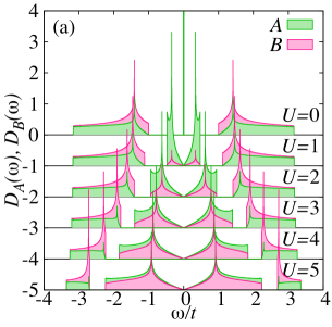
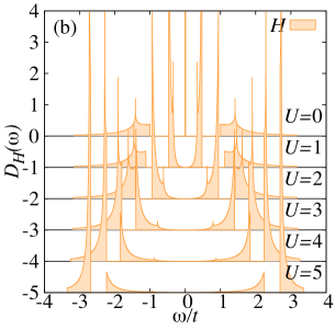
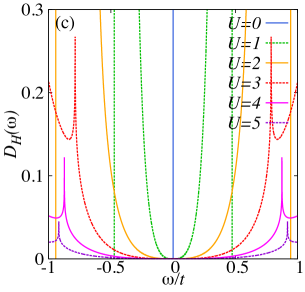
Figure 14: (color online) Orbital resolved density of states (a) $D_{A/B}(\omega)$ and (b) $D_{H}(\omega)$ for various values of $U$ (indicated in the figures) with $t_{sp}/t=1$ obtained by the Hubbard-I approximation. Notice that the results are shifted by $U$ for clarity. (c) The enlarged plot of $D_{H}(\omega)$ in (b) near the Fermi energy. The diverging density of states due to the flat band for $U=0$ is represented by the vertical line at $\omega=0$. The Fermi energy $E_{\rm F}$ is located at $\omega=0$.

The characteristic features of the spectral weight redistribution are summarized as follows. The flat band which appears in the noninteracting limit (see Sec. II.2) causes a delta function peak at $\omega=0$ in $D_{A}(\omega)$ and $D_{H}(\omega)$, but not in $D_{B}(\omega)$. However, once the Coulomb interaction $U$ is introduced, the flat band in $D_{A}(\omega)$ splits into two bands around the Fermi energy to form a “Dirac band” with the massless Dirac quasiparticle dispersion (see Fig. 13 and also Fig. 16). It is also noticed in Fig. 14(a) that the high energy spectral weight in $D_{A}(\omega)$ for $|\omega|\gtrsim\Delta_{c}$, where

$$\Delta_{c}=\sqrt{\left(\frac{U}{2}\right)^{2}+t_{sp}^{2}}=\frac{1}{2}\frac{v_{0}}{v_{\rm F}}U$$ (42)

is the lower (upper) bound of the upper (lower) Hubbard band at $K$ and $K^{\prime}$ points, is transferred to the low energy region to participate in the formation of the massless Dirac quasiparticles. Simultaneously, the spectral weight $D_{B}(\omega)$ for $B$ orbital in the low energy region $|\omega|<\Delta_{c}$ is gradually transferred from the upper and lower Hubbard bands located in the high energy region $|\omega|\gtrsim\Delta_{c}$, and the contribution of $B$ orbital to the “Dirac band” becomes as significant as that of $A$ orbital for larger values of $U$. Indeed, $D_{A}(\omega)\approx D_{B}(\omega)$ in the “Dirac band” for $|\omega|<\Delta_{c}$ when $U/t\gtrsim 5$. On the other hand, as shown in Figs. 14(b) and 14(c), the spectral weight $D_{H}(\omega)$ for $H$ orbital loses its intensity in the low energy region near the Fermi energy and the large spectral weights are piled up in rather narrow high energy regions, exhibiting a typical localized incoherent feature. This spectral weight redistribution enhances the coherent hybridization between $A$ and $B$ orbitals in the low energy region. Therefore, the participation of $B$ orbital together with the disengagement of $H$ orbital in the low energy excitations is essential to form the massless Dirac quasiparticles near the Fermi energy.

It is indeed noticed in Fig. 14(a) that $D_{A}(\omega)$ and $D_{B}(\omega)$ both exhibit the linearly vanishing density of states near the Fermi energy, a characteristic feature of the massless Dirac dispersion. It is well known that the Van Hove singularity appears in the DOS at $\omega=\pm t$, i.e., $\omega=\pm 2v_{0}/\sqrt{3}$, for the pure graphene model, as shown in Fig. 15(c). Similarly, we find in Fig. 14 that the Van Hove singularity appears exactly at $\omega/t=\pm v_{\rm F}/v_{0}$, i.e., $\omega=\pm 2v_{\rm F}/\sqrt{3}$, even for the periodic Anderson model, indicating that the low energy band for $|\omega|<\Delta_{c}$ can in fact be regarded as an effective pure graphene band with the renormalized Dirac Fermi velocity $v_{\rm F}$.

As shown in Fig. 15(a), we also find that the slope of $D_{B}(\omega)$ around the Fermi energy is independent of $U/t$ and is identical to that for the pure graphene model. The density of states $D_{0}(\omega)$ per orbital for the pure graphene model is shown in Fig. 15(c) and can be evaluated as

$$D_{0}(\omega) = -\frac{1}{\pi N_{a}}\sum_{\mathbf{k}}\sum_{\sigma}\lim_{\eta\rightarrow 0^{+}}\Im G_{0}^{\alpha\alpha}(\mathbf{k},\omega+\mathrm{i}\eta)$$ (43)

$$= \frac{1}{N_{a}}\sum_{\mathbf{k}}\left\{\delta(\omega-|\gamma_{\mathbf{k}}|)+\delta(\omega+|\gamma_{\mathbf{k}}|)\right\},$$

where

$$G_{0}^{\alpha\alpha}(\mathbf{k},\omega)=\frac{1}{2}\left(\frac{1}{\omega-|\gamma_{\mathbf{k}}|}+\frac{1}{\omega+|\gamma_{\mathbf{k}}|}\right)$$ (44)

is the diagonal element of the noninteracting single-particle Green’s function with orbital $\alpha\,(=A$ and $B$) and spin $\sigma\,(=\uparrow$ and $\downarrow)$ for the pure graphene model. Indeed, one can find within the Hubbard-I approximation that the DOS for $B$ orbital near the Fermi energy is

$$D_{B}(\omega)=\frac{\sqrt{3}}{2\pi}\frac{|\omega|}{v_{0}^{2}}=\frac{2\sqrt{3}}{3\pi}\frac{|\omega|}{t^{2}}$$ (45)

for $|\omega|\sim 0$, exactly the same slope of the linearly increasing DOS for the pure graphene model Neto2009RMP and independent of the value of $U$. As shown in Fig. 15(b), the same results are also found in the CPT calculations for the PM state.

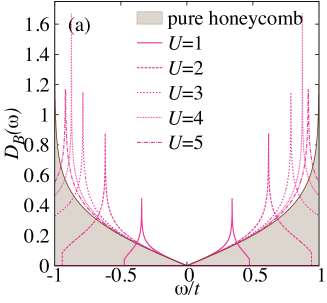
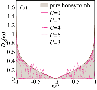
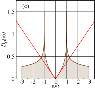
Figure 15: (color online) Density of states $D_{B}(\omega)$ for $B$ orbital near the Fermi energy for various values of $U$ (indicated in the figures) with $t_{sp}/t=1$ obtained by (a) the Hubbard-I approximation and (b) the CPT. The CPT calculations are for the PM state at $T/t=0.025$ using the 6-site cluster (containing 2 unit cells) with a Lorentzian broadening of $\eta/t=0.005$. For comparison, density of states $D_{0}(\omega)$ per orbital for the pure graphene model is plotted in (c) and also indicated by a shaded region in (a) and (b). Red straight lines ($\frac{2\sqrt{3}}{3\pi}\frac{|\omega|}{t^{2}}$) in (c) represent the initial slope of $D_{0}(\omega)$ around the Fermi energy $E_{\rm F}$ at $\omega=0$.

We can now show that the spectral weight $\rho^{BB}_{\nu,\mathbf{k}}$ for $B$ orbital at the Dirac points, i.e., at $K$ (and also $K^{\prime}$) point on the Fermi energy, is related to the Dirac Fermi velocity $v_{\rm F}$ via

$$\rho^{BB}_{2/3,K(K^{\prime})}=\frac{1}{2}\left(\frac{v_{\rm F}}{v_{0}}\right)^{2}.$$ (46)

From Eq. (41), the slope of the DOS near the Fermi energy is evaluated as

$$\lim_{\omega\to 0}\frac{D_{B}(\omega)}{\omega} = \lim_{\omega\to 0}\frac{4}{\omega V_{\rm BZ}}\int_{0}^{\Lambda}\mathrm{d}\kappa\,\kappa\int_{0}^{2\pi}\mathrm{d}\theta$$ (49)

$$\times \left[\rho_{2,K}^{BB}\,\delta\left(\omega-v_{\rm F}\kappa\right)+\rho_{3,K}^{BB}\,\delta\left(\omega+v_{\rm F}\kappa\right)\right]$$

$$= \left\{\begin{array}[]{ll}\displaystyle\frac{\sqrt{3}}{\pi}\frac{\rho^{BB}_{2,K}}{v_{\rm F}^{2}}&(\omega\to 0^{+}),\\ \displaystyle-\frac{\sqrt{3}}{\pi}\frac{\rho^{BB}_{3,K}}{v_{\rm F}^{2}}&(\omega\to 0^{-}),\end{array}\right.$$

where the factor $4$ on the right hand side of the first line accounts for the contributions to the DOS of the four emergent Dirac cones with the low-energy linear energy dispersions in the neighborhoods of $K$ and $K^{\prime}$ points, including the spin degeneracy. $V_{\rm BZ}=8\pi^{2}/\sqrt{3}$ is the volume of the Brillouin zone, $\Lambda$ is a positive cut-off momentum within which the low energy dispersion is approximated linear in momentum around $K$ and $K^{\prime}$ points, and $0^{+(-)}$ is positive (negative) infinitesimal. We have also used that

$$\frac{1}{N_{a}}\sum_{\mathbf{k}}\cdots=\frac{1}{V_{\rm BZ}}\int\mathrm{d}^{2}k\cdots.$$ (50)

Since we can show form Eq. (43) that $\rho^{BB}_{2,K}=\rho^{BB}_{3,K}=1/2$ and $v_{\rm F}=v_{0}$ in Eq. (49) for the pure graphene model, the fact that the slope of $D_{B}(\omega)$ near the Fermi energy is the same as that of $D_{0}(\omega)$ naturally leads to Eq. (46). This is indeed derived analytically below in Eq. (54).

IV.2.6 Spectral weight at the Dirac points

Although the density of states $D_{\alpha}(\omega)$ vanishes at $\omega=0$, the spectral weight $\boldsymbol{\rho}_{\nu,\mathbf{k}}$ itself is finite even at $\omega=0$ for ${\mathbf{k}}=$ $K$ and $K^{\prime}$. Here, we derive the analytical expression of the spectral weight at $K$ point where the massless Dirac dispersions emerge. Because $\gamma_{\mathbf{k}=K}=0$, the spectral weight at $K$ point is determined only by $U$ and $t_{sp}$. Indeed, the poles of the single-particle Green’s function in Eq. (29) are located at $\omega_{1/4,K}=\pm\Delta_{c}$ and $\omega_{2/3,K}=0$. Therefore, from Eqs. (38) and (39), the spectral weights $\rho^{\alpha\alpha}_{\nu,K}$ at $K$ point are given as

$$\rho_{1/4,K}^{AA} = \rho_{2/3,K}^{HH}=0,$$ (51)

$$\rho_{2/3,K}^{AA} = \rho_{1/4,K}^{HH}=\frac{1}{2},$$ (52)

$$\rho_{1/4,K}^{BB} = \frac{1}{2}\left\{1-\left(\frac{v_{\rm F}}{v_{0}}\right)^{2}\right\},$$ (53)

$$\rho_{2/3,K}^{BB} = \frac{1}{2}\left(\frac{v_{\rm F}}{v_{0}}\right)^{2}.$$ (54)

The spectral weight at the Dirac point, corresponding to $\nu=2$ and $3$, is indeed finite even though the density of states is zero at the Fermi energy.

Since the spectral weight $\rho_{\nu,K}^{\alpha\alpha}$ considered here is related to the spectral weight $\rho_{K}^{\alpha\alpha}$ of the single-particle excitation spectrum $A^{\alpha\alpha}_{\sigma}({\mathbf{k}}=K,\omega=0)$, defined in Eq. (11), as

$$\rho_{K}^{\alpha\alpha}=\rho_{2,K}^{\alpha\alpha}+\rho_{3,K}^{\alpha\alpha},$$ (55)

we find that $\rho^{BB}_{K}$ is highly correlated to $v_{\rm F}$, i.e., $\rho_{K}^{BB}=(v_{\rm F}/v_{0})^{2}$, exactly the same relation found by the CPT for the PM state in Fig. 11, and monotonically increases with increasing $U$ as $v_{\rm F}$ also monotonically increases (see Fig. 8). On the other hand, we find that $\rho_{K}^{AA}=1$ and $\rho_{K}^{HH}=0$, irrespectively of the value of $U$. This is also in good agreement with that obtained by the CPT for the PM state. These results therefore suggest that the involvement of $B$ orbital in the low-energy excitations, which is absent in the noninteracting limit, is essential to form the emergent massless Dirac quasiparticles.

Now, using the spectral weights $\rho^{\alpha\alpha}_{\nu,K}$ in Eqs. (51)–(54), we can readily obtain within the Hubbard-I approximation the single-particle Green’s function at $K$ point as

$$G_{\sigma}^{AA}(K,\omega) = \frac{1}{\omega},$$ (56)

$$G_{\sigma}^{BB}(K,\omega) = \left(\frac{v_{\rm F}}{v_{0}}\right)^{2}\frac{1}{\omega}+\frac{1}{2}\left\{1-\left(\frac{v_{\rm F}}{v_{0}}\right)^{2}\right\}$$ (57)

$$\times \left(\frac{1}{\omega-\Delta_{c}}+\frac{1}{\omega+\Delta_{c}}\right),$$

$$G_{\sigma}^{HH}(K,\omega) = \frac{1}{2}\left(\frac{1}{\omega-\Delta_{c}}+\frac{1}{\omega+\Delta_{c}}\right).$$ (58)

From these analytical forms, we can find several characteristic features of the single-particle excitations. First, $G_{\sigma}^{AA}(K,\omega)$ does not depend on $U$ and it remains in the same form as in the noninteracting case. Namely, it has a single pole at zero energy ($\omega=0$) and its spectral weight is one. Second, $G_{\sigma}^{BB}(K,\omega)$ has a pole at $\omega=0$ with its spectral weight proportional to the square of the Dirac Fermi velocity $v_{\rm F}$, i.e., $\left(\frac{v_{\rm F}}{v_{0}}\right)^{2}=\frac{U^{2}}{U^{2}+4t_{sp}^{2}}$. The other two poles are located at $\omega=\pm\Delta_{c}$ and their spectral weights are both $\frac{1}{2}\left\{1-\left(\frac{v_{\rm F}}{v_{0}}\right)^{2}\right\}$. Therefore, as $U$ increases, the spectral weight is transferred from the high energy poles at $\omega=\pm\Delta_{c}$ in the upper and lower Hubbard bands to the zero energy one in the Dirac band. Third, $G_{\sigma}^{HH}(K,\omega)$ has no poles at $\omega=0$ for any finite value of $U$, but at $\omega=\pm\Delta_{c}$.

IV.2.7 Single-particle excitation spectrum

From Eq. (36), the single-particle excitation spectrum $A^{\alpha\alpha}_{\sigma}(\mathbf{k},\omega)$ for $\alpha$ orbital is given as

$$A^{\alpha\alpha}_{\sigma}(\mathbf{k},\omega)=\sum_{\nu=1}^{4}\rho^{\alpha\alpha}_{\nu,\mathbf{k}}\delta(\omega-\omega_{\nu,\mathbf{k}}).$$ (59)

Since the poles $\omega_{\nu,\mathbf{k}}$ as well as the spectral weights $\rho^{\alpha\alpha}_{\nu,\mathbf{k}}$ are all known analytically in Eqs. (29), (38), and (39), the calculation of the single-particle excitation spectrum $A^{\alpha\alpha}_{\sigma}(\mathbf{k},\omega)$ is straightforward and the results for various values of $U$ are shown in Fig. 16. We can clearly find in Fig. 16 that (i) the flat band which is present only at $U=0$ evolves into the Dirac band with the massless Dirac dispersions emerging around $K$ and $K^{\prime}$ points near the Fermi energy, (ii) the Dirac points are located exactly at the Fermi level and momentum ${\mathbf{k}}=K$ and $K^{\prime}$, (iii) the contribution of $B$ orbital to the Dirac band becomes increasingly significant with increasing $U$, while $H$ orbital does not participate in the formation of the massless Dirac dispersion, and (iv) the highest and lowest bands which display the massive Dirac dispersions near $K$ and $K^{\prime}$ points at $U=0$ evolve respectively into the upper and lower Hubbard bands in the high energy regions for $|\omega|\gtrsim\Delta_{c}$. These characteristic features are in good qualitative agreement with those obtained by the CPT for the PM state shown in Fig. 7.

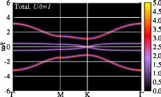
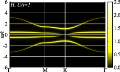
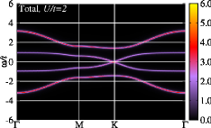
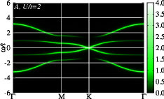
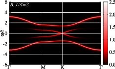
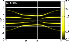
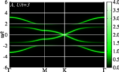
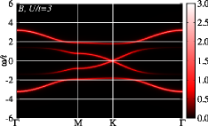
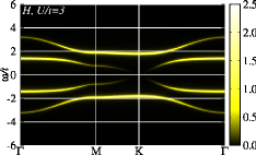
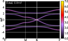
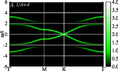
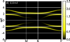
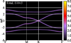
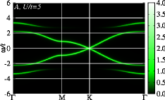
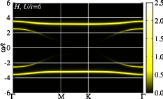
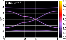
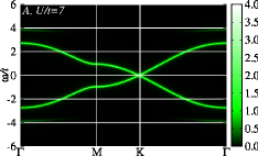
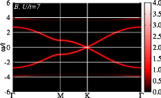
Figure 16: (color online) Single-particle excitation spectra for $U/t=0,1,\cdots,7$ (from top to bottom) and $t_{sp}/t=1$ obtained by the Hubbard-I approximation. $A_{\sigma}(\mathbf{k},\omega)=\sum_{\alpha}A^{\alpha\alpha}_{\sigma}(\mathbf{k},\omega)$, $A^{AA}_{\sigma}(\mathbf{k},\omega)$, $A^{BB}_{\sigma}(\mathbf{k},\omega)$, and $A^{HH}_{\sigma}(\mathbf{k},\omega)$ are shown from left to right panels. Here, we only show the spectra $A^{\alpha\alpha}_{\uparrow}(\mathbf{k},\omega)$ for up electrons, which are exactly the same as $A^{\alpha\alpha}_{\downarrow}(\mathbf{k},\omega)$. A Lorentzian broadening of $\eta/t=0.05$ is used. The spectral intensity is indicated by a color bar in each figure. Note that the different intensity scales are used for different figures. The Fermi energy $E_{\rm F}$ is located at $\omega=0$.

Although it is already convincing that the contribution of $B$ orbital to the low energy excitations is essential for the emergent massless Dirac quasiparticles, here we quantify the low energy bonding character between $A$ and $B$ orbitals and examine how this quantity evolves with increasing $U$ within the Hubbard-I approximation. For this purpose, let us define the following effective dynamical bonding strength between $A$ and $B$ orbitals

$$L_{AB}=\frac{1}{N_{a}}\sum_{\mathbf{k},\sigma}\int_{-\Delta_{c}}^{0}d\omega\left|A^{AB}_{\sigma}(\mathbf{k},\omega)+A^{BA}_{\sigma}(\mathbf{k},\omega)\right|,$$ (60)

where $-\Delta_{c}$ is the upper bound of the lower Hubbard band given in Eq. (42). Note that this quantity becomes $T_{AB}=\sum_{\sigma}|\langle c^{\dagger}_{{\mathbf{r}}_{i}\sigma A}c_{{\mathbf{r}}_{i}\sigma B}+{\rm H.c.}\rangle|$ if the lower bound of the integral is extended to $-\infty$. As shown in Fig. 17, we find that although $T_{AB}$ is almost constant and does not depend strongly on $U$, $L_{AB}$ is rather sensitive to $U$ and monotonically increases from zero. This clearly demonstrates that the low energy bonding between $A$ and $B$ orbitals becomes stronger as the massless Dirac quasiparticles develops with increasing $U$, which is accompanied by the large spectral weight redistribution from the upper and lower Hubbard bands to the Dirac band.

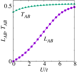
Figure 17: (color online) $U$ dependence of the effective dynamical bonding strength $L_{AB}$ and $T_{AB}$ (see the text for definition) for $t_{sp}/t=1$ calculated using the Hubbard-I approximation.

IV.3 Chiral symmetry in single-particle excitations

It is well known in the single-particle theory that for a bipartite system with no hopping between two different sites on the same sublattice, there exist zero-energy states at least as many as the difference of the number of sites on each sublattice Lieb ; Hatsugai2007 ; Hatsugai2013 ; Hatsugai2014 . For example, the flat band found in the noninteracting limit of the periodic Anderson model $\mathcal{H}$ is a typical case because the number of sites on each sublattice is different (i.e., sublattice imbalanced) by one per unit cell, thus leading to at least one zero-energy state at each momentum, as discussed in Sec. II.2. On the other hand, this theorem does not predict the existence of the four Dirac cones with eight zero-energy states in the pure graphene model (including the spin degeneracy) as the pure graphene model contains the same number of sites on each sublattice. Instead, the four Dirac cones at $K$ and $K^{\prime}$ points in the pure graphene model are protected by the time-reversal symmetry, 120^∘-rotational symmetry, and sublattice (or, equivalently, inversion) symmetry Bernevig .

Here, we argue that the quasiparticle excitations in the PM phase of the periodic Anderson model dynamically recover the sublattice balance, thus eliminating a trivial zero-energy state, and the Dirac cone like dispersions with point contacts at zero energy is protected by the electron correlation.

For this purpose, we shall construct an effective Hamiltonian in a quadratic form of fermion quasiparticle operators, which reproduces the single-particle excitations obtained by the Hubbard-I approximation, and follow the chiral symmetry argument given in Refs. Hatsugai2007 ; Hatsugai2013 ; Hatsugai2014 .

By introducing an auxiliary orbital $X$, we construct the following effective Hamiltonian:

$$\mathcal{H}_{\text{H-I}}=\sum_{\mathbf{k},\sigma}\tilde{\boldsymbol{c}}_{\mathbf{k}\sigma}^{\dagger}\left(\begin{array}[]{cccc}0&\gamma_{\mathbf{k}}&0&0\\ \gamma^{*}_{\mathbf{k}}&0&t_{sp}&0\\ 0&t_{sp}&0&U/2\\ 0&0&U/2&0\end{array}\right)\tilde{\boldsymbol{c}}_{\mathbf{k}\sigma},$$ (61)

where fermion creation operators $\tilde{\boldsymbol{c}}_{\mathbf{k}\sigma}^{\dagger}=(\tilde{c}_{\mathbf{k}\sigma A}^{\dagger}\,\tilde{c}_{\mathbf{k}\sigma B}^{\dagger}\,\tilde{c}_{\mathbf{k}\sigma H}^{\dagger}\,\tilde{c}_{\mathbf{k}\sigma X}^{\dagger})$ in the momentum space describe the quasiparticles, not the bare electrons, in the Hubbard-I approximations. Here, the dynamical electron correlation in the Hubbard-I approximation is represented as the hybridization between the auxiliary orbital $X$ and the hydrogen orbital $H$ with the hybridization strength $U/2$ (see Fig. 18). The Mott gap between the upper and lower Hubbard bands in the Hubbard-I approximation is then interpreted as a single-particle hybridization gap generated by introducing $X$ orbital. Indeed, we can show that the eigenvalues of $\mathcal{H}_{\text{H-I}}$ coincide with $\omega_{\nu,\mathbf{k}}$ ($\nu=1,2,3$, and $4$) in the Hubbard-I approximation (see Sec. IV.2.2). The similar interpretation of the Mott gap is recently emphasized by Sakai et al. in the context of high-temperature cuprate superconductors Sakai2014 . The analysis of the effective Hamiltonian $\mathcal{H}_{\text{H-I}}$ based on the Brillouin-Wigner perturbation theory is given in Appendix E.

The spectral weight of the single-particle Green’s function obtained by the Hubbard-I approximation in Eq. (36) can also be reproduced from the eigenstates ${\boldsymbol{\gamma}}^{\dagger}_{{\mathbf{k}}\sigma}$ of $\mathcal{H}_{\text{H-I}}$, i.e.,

$$\mathcal{H}_{\text{H-I}}=\sum_{\mathbf{k},\sigma}{\boldsymbol{\gamma}}^{\dagger}_{{\mathbf{k}}\sigma}\left(\begin{array}[]{cccc}\omega_{1,\mathbf{k}}&0&0&0\\ 0&\omega_{2,\mathbf{k}}&0&0\\ 0&0&\omega_{3,\mathbf{k}}&0\\ 0&0&0&\omega_{4,\mathbf{k}}\end{array}\right){\boldsymbol{\gamma}}_{{\mathbf{k}}\sigma},$$ (62)

where

$${\boldsymbol{\gamma}}^{\dagger}_{{\mathbf{k}}\sigma}=\tilde{\boldsymbol{c}}_{\mathbf{k}\sigma}^{\dagger}\boldsymbol{U}_{\mathbf{k}}$$ (63)

and

$$\boldsymbol{U}_{\mathbf{k}}=\left(\begin{array}[]{cccc}u_{1,\mathbf{k}}^{A}&u_{2,\mathbf{k}}^{A}&u_{3,\mathbf{k}}^{A}&u_{4,\mathbf{k}}^{A}\\ u_{1,\mathbf{k}}^{B}&u_{2,\mathbf{k}}^{B}&u_{3,\mathbf{k}}^{B}&u_{4,\mathbf{k}}^{B}\\ u_{1,\mathbf{k}}^{H}&u_{2,\mathbf{k}}^{H}&u_{3,\mathbf{k}}^{H}&u_{4,\mathbf{k}}^{H}\\ u_{1,\mathbf{k}}^{X}&u_{2,\mathbf{k}}^{X}&u_{3,\mathbf{k}}^{X}&u_{4,\mathbf{k}}^{X}\end{array}\right),$$ (64)

by simply setting the $X$ components in $\boldsymbol{U}_{\mathbf{k}}$ to be zero. The $\nu$-th band component of the spectral weight $\boldsymbol{\rho}_{\nu,\mathbf{k}}$ in the Hubbard-I approximation is simply obtained as

$$\rho_{\nu,\mathbf{k}}^{\alpha\beta}=(u_{\nu,\mathbf{k}}^{\alpha})^{*}u_{\nu,\mathbf{k}}^{\beta},$$ (65)

where $\alpha,\beta=A,B,$ and $H$. Notice that the unitarity of $\boldsymbol{U}_{\mathbf{k}}$ ensures the spectral weight sum rule of the Hubbard-I approximation in Eq. (40).

We now introduce the sublattice indexes $a$ and $b$ such that $A$ and $H$ sites belong to $a$ sublattice, and $B$ and $X$ sites belong to $b$ sublattice. By rearranging the rows and columns of the Hamiltonian matrix in Eq. (61), the effective Hamiltonian is

$$\mathcal{H}_{\text{H-I}} = \sum_{\mathbf{k}\sigma}\left(\tilde{c}_{\mathbf{k}\sigma A}^{\dagger}\,\tilde{c}_{\mathbf{k}\sigma H}^{\dagger}\,\tilde{c}_{\mathbf{k}\sigma B}^{\dagger}\,\tilde{c}_{\mathbf{k}\sigma X}^{\dagger}\right)$$ (72)

$$\quad\quad\quad\times\left(\begin{array}[]{cc}\boldsymbol{O}&\boldsymbol{T}_{\mathbf{\mathbf{k}}}\\ \boldsymbol{T}_{\mathbf{\mathbf{k}}}^{\dagger}&\boldsymbol{O}\end{array}\right)\left(\begin{array}[]{c}\tilde{c}_{\mathbf{k}\sigma A}\\ \tilde{c}_{\mathbf{k}\sigma H}\\ \tilde{c}_{\mathbf{k}\sigma B}\\ \tilde{c}_{\mathbf{k}\sigma X}\end{array}\right),$$

where

$$\boldsymbol{T}_{\mathbf{k}}=\left(\begin{array}[]{cc}\gamma_{\mathbf{k}}&0\\ t_{sp}&U/2\end{array}\right)$$ (73)

represents the hopping between sites on different sublattices.

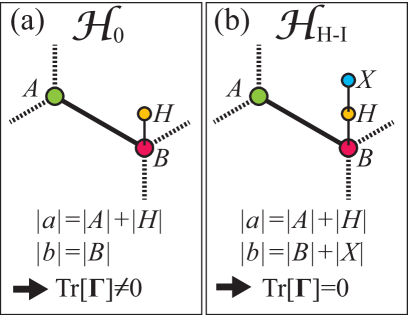
Figure 18: (color online) Schematic representations for (a) the periodic Anderson model $\mathcal{H}$ in the noninteracting limit and (b) the effective Hamiltonian $\mathcal{H}_{\text{H-I}}$ where the electron correlation $U$ is represented as the hybridization between $H$ orbital and auxiliary $X$ orbital. Both models are defined on bipartite lattices with the hopping between different sublattices, and preserve the chiral symmetry. The $A$-$B$ sublattice symmetry (the Hamiltonian is invariant under the exchange of $A$ and $B$ orbitals) as in the pure graphene model is apparently broken in both models. Although the sublattice balance is also broken in model (a), i.e., $|a|\not=|b|$, it is preserved in model (b) due to the presence of auxiliary $X$ orbital.

We can now show that $\mathcal{H}_{\text{H-I}}$ is chiral symmetric. Let us define $|a|=|A|+|X|$ and $|b|=|B|+|H|$ as the number of orbitals belonging to $a$ and $b$ sublattices, respectively, and

$$\boldsymbol{H}_{\mathbf{k}}=\left(\begin{array}[]{cc}\boldsymbol{O}&\boldsymbol{T}_{\mathbf{\mathbf{k}}}\\ \boldsymbol{T}_{\mathbf{\mathbf{k}}}^{\dagger}&\boldsymbol{O}\end{array}\right)$$ (74)

is a $4\times 4$ matrix in Eq. (72). Then, following the argument given by Hatsugai et al. Hatsugai2013 , $\mathcal{H}_{\text{H-I}}$ is said to be chiral symmetric if a matrix $\boldsymbol{\Gamma}$ exists such that

$$\left\{\boldsymbol{H}_{\mathbf{k}},\boldsymbol{\Gamma}\right\}=\boldsymbol{H}_{\mathbf{k}}\boldsymbol{\Gamma}+\boldsymbol{\Gamma}\boldsymbol{H}_{\mathbf{k}}=\boldsymbol{O},$$ (75)

$$(\boldsymbol{\Gamma})^{2}=\boldsymbol{I},\,{\rm and}$$ (77)

$${\rm Tr}[\boldsymbol{\Gamma}]=|a|-|b|,$$

where $\boldsymbol{O}$ ($\boldsymbol{I}$) is a null (unit) matrix. Equations (75) and (77) remind us the Dirac matrices in relativistic quantum mechanics, although the Dirac matrices must be traceless, instead of Eq. (77). We can easily find that for any $\mathbf{k}$

$$\boldsymbol{\Gamma}=\left(\begin{array}[]{cc}\boldsymbol{I}&\boldsymbol{O}\\ \boldsymbol{O}&-\boldsymbol{I}\end{array}\right)$$ (78)

is the matrix which defines the chiral symmetry of $\mathcal{H}_{\text{H-I}}$. The $\boldsymbol{\Gamma}$ matrix is the matrix representation of chiral operator and represents the basis transformation, $\tilde{c}_{\mathbf{k}\sigma A(H)}\to\tilde{c}_{\mathbf{k}\sigma A(H)}$ and $\tilde{c}_{\mathbf{k}\sigma B(X)}\to-\tilde{c}_{\mathbf{k}\sigma B(X)}$. Equation (75) or equivalently $\boldsymbol{\Gamma}\boldsymbol{H}_{\mathbf{k}}\boldsymbol{\Gamma}^{-1}=-\boldsymbol{H}_{\mathbf{k}}$ thus implies that $\mathcal{H}_{\text{H-I}}$ changes the sign by this transformation. Notice also that $\boldsymbol{\Gamma}$ in Eq. (78) is a traceless matrix, i.e., ${\rm Tr}[\boldsymbol{\Gamma}]=|a|-|b|=0$ in Eq. (77).

It should be recalled here that ${\rm Tr}[\boldsymbol{\Gamma}]=|a|-|b|$ represents the difference of the number of sites belonging to $a$ and $b$ sublattices, and gives the number of zero-energy states, as first pointed out by Lieb Lieb (see also Ref. Hatsugai2013 ). Indeed, we can find a $3\times 3$ matrix $\boldsymbol{\Gamma}$ even for the periodic Anderson model in the noninteracting limit, i.e., $\mathcal{H}_{0}$ in Eq. (3), which satisfies Eqs. (75)–(77), but its trace is ${\rm Tr}[\boldsymbol{\Gamma}]=|a|-|b|=1$. This immediately indicates the presence of the flat band due to the sublattice imbalance, as already discussed in Sec. II.2. The tracelessness of $\boldsymbol{\Gamma}$ in Eq. (78) for $\mathcal{H}_{\text{H-I}}$ thus implies that these trivial zero-energy states are absent, which is similar to the cases of the pure graphene model and also the relativistic particle in the Dirac equation, where the chiral symmetry is preserved.

It is now easy to show that the “non-trivial” zero-energy states exist only at $K$ and $K^{\prime}$ points for $\mathcal{H}_{\text{H-I}}$ as long as the electron correlation $U$ is finite. Since $t_{sp}$ and $U$ are independent of $\mathbf{k}$ and $\gamma_{\mathbf{k}}=0$ only at $K$ and $K^{\prime}$ points, we can readily find that

$${\rm rank}\,\boldsymbol{T_{\mathbf{k}}}=\left\{\begin{array}[]{ll}1\quad\text{($\mathbf{k}=K,K^{\prime}$)}\\ 2\quad\text{(otherwise)}\end{array}\right.$$ (81)

provided that $t_{sp}$ and $U$ are both finite. It is then immediately followed that

$${\rm rank}\,\boldsymbol{H_{\mathbf{k}}}=\left\{\begin{array}[]{ll}2\quad\text{($\mathbf{k}=K,K^{\prime}$)}\\ 4\quad\text{(otherwise).}\end{array}\right.$$ (84)

Equation (84) therefore guarantees the existence of two zero-energy modes at $K$ ($K^{\prime}$) point, which represent the point contact of the single-particle excitations exactly at Fermi energy. In other words, the finite electron correlation $U$ and the chiral symmetry of ${\mathcal{H}}_{\text{H-I}}$ with ${\rm Tr}[{\mathbf{\Gamma}}]=0$ permit the point contacts of the single-particle excitations to appear only at $K$ and $K^{\prime}$ points. We should note that the argument given here is a direct extension of the pure graphene model Hatsugai2014 to the four orbital model ${\mathcal{H}}_{\text{H-I}}$.

V Discussion

First, we should remark on the Hubbard-I approximation which has been repeatedly proved to successfully reproduce qualitatively and sometimes quantitatively the results obtained by the CPT for the PM state of the periodic Anderson model studied here. To understand the success of the Hubbard-I approximation, we should recall that there exists the flat band in the noninteracting limit, which is exactly half-filled. This flat band structure prohibits any perturbative treatment of $U$ since even a small $U$ should be regard as the strong correlation. This explains why the Hubbard-I approximation, which is usually a good approximation in the atomic (i.e., strong coupling) limit, gives the satisfactory results even for small $U$.

Second, the emergent massless Dirac quasiparticles found here should be sharply contrasted to the recently discussed massless Dirac dispersion generated by band engineering Ishizuka2012 ; Lin2013 . Our finding differs from the previous reports in the following aspects: (i) while the electron correlation induces the massless Dirac quasiparticles in our case, breaking the spatial symmetry is essential to generate the massless Dirac dispersion in the band engineering, and (ii) the Dirac point appears exactly at the Fermi energy in our case, but it is generally away from the Fermi energy in the band engineered Dirac dispersion. To the best of our knowledge, this is the first example of the emergent massless Dirac quasiparticles due to dynamical electron correlations without breaking any spatial symmetry.

Third, let us briefly discuss the experimental implications of our results. We have studied the half-depleted periodic Anderson model on the honeycomb lattice at half filling, which can be considered as the simplest model for the single-side hydrogenated graphene. Recently, Ray et al. Ray2014 reported a ferromagnetism in a partially hydrogenated graphene on the graphite substrate. Their observation of the ferromagnetism is consistent with our ground state calculations. Although Lieb’s theorem can not directly applied to the periodic Anderson model studied here, we have shown in Sec. III.1 and Appendix C that the FM ground state found in our calculations is smoothly connected to the Lieb-Mattis type ferromagnetism. Therefore, we attribute the ferromagnetism observed experimentally to the Lieb-Mattis type ferromagnetism.

Another possible experiment which is relevant to our calculations is a graphene sheet on transition metal substrates. Varykhalov et al. Varykhalov2012 reported angle-resolved photoemission spectroscopy (ARPES) experiments for graphene deposited on Ni(111) and Co(0001) surfaces. In these systems, the sublattice symmetry of graphene is apparently broken. This is because the carbon atoms on $B$ sublattice of the graphene sheet locate on top of the transition metal atoms of the substrate, whereas the carbon atoms on $A$ sublattice are placed on top of the interstitial sites of the transition metal atoms. Therefore, the carbon $2p_{z}$ orbitals on $B$ sublattice hybridize strongly with the transition metal $3d$ orbitals, but the hybridization between the carbon atoms on $A$ sublattice and the transition metal atoms is rather weak. In spite of the broken sublattice symmetry, they have observed in their ARPES experiments the linearly dispersing single-particle excitations with the Dirac point about 2.8 eV below the Fermi energy Varykhalov2012 . The deviation of the Dirac point from the Fermi energy might be understood simply as a consequence of the electron transfer from the substrate. Since the most simplest model for these systems is the half-depleted periodic Anderson model studied here, their observation can be understood as the emergent massless Dirac quasiparticles induced by the electron correlation of transition metals. However, more detailed study is highly desired for quantitative comparison.

VI Summary

Using the VCA and the CPT, we have studied the finite temperature phase diagram of the half-depleted periodic Anderson model at half-filling for a model of graphone, i.e., the single-side hydrogenated graphene. We have found that the ground state is FM as long as the electron correlation $U$ on the hydrogen impurity sites is finite. Although the single-particle excitations with the same spin are gapped, the quasiparticle dispersions with the opposite spins touch at $K$ and $K^{\prime}$ points. Therefore, this FM state is semi-metallic. We have discussed the relevance of Lieb’s theorem to the periodic Anderson model, and shown, with the help of numerically exactly diagonalizing small clusters, that the FM ground state found here is smoothly connected to the Lieb-Mattis type ferromagnetism. We have also shown in the strong coupling limit that the FM state displays the linear spin wave dispersion at zero temperature, rather than the quadratic spin wave dispersion often observed in the FM state. This is simply because of the peculiar Dirac like electron energy dispersion of the conduction band. However, we have found that the spin wave dispersion becomes quadratic at finite temperatures, thus implying that the FM state is stable only at zero temperature, consistent with Mermin-Wagner theorem.

Indeed, we have found using the VCA that the FM state is fragile against thermal fluctuations, and the finite temperature phase diagram is dominated by the PM phase. More surprisingly, our CPT calculations have revealed that the massless Dirac quasiparticles emerge at $K$ and $K^{\prime}$ points with the Dirac points exactly at the Fermi energy, once the electron correlation $U$ is introduced in the PM state. This should be contrasted with the quadratic quasiparticle dispersions in the FM phase. We have shown that the emergent massless Dirac quasiparticles in the PM phase can be reproduced in the Hubbard-I approximation. Moreover, we have found that the formation of the emergent massless Dirac quasiparticles is accompanied with the spectral weight redistribution of the single-particle excitations, involving a large energy scale of $U$. In fact, we have found in both CPT and Hubbard-I approximation that the single-particle spectral weight $\rho_{K}^{BB}$ for $B$ orbital at the Dirac point is proportional to the square of the Dirac Fermi velocity $v_{\rm F}$, i.e., $\rho_{K}^{BB}=(v_{\rm F}/v_{0})^{2}$, where $v_{\rm F}$ is zero when $U=0$ and monotonically increases with $U$. This universal relation expresses that the involvement of $B$ orbital in the low-energy excitations is essential for the formation of the emergent massless Dirac quasiparticles. Constructing the effective quasiparticle Hamiltonian, we have argued that the Dirac cones with the point contacts at $K$ and $K^{\prime}$ points are protected by the electron correlation $U$. Our finding therefore represents the first example of the emergence of massless Dirac quasiparticles induced by the electron correlation without breaking any spatial symmetry.

Appendix A Linear spin wave analysis for the FM state in the strong coupling limit

In this Appendix, we consider the large $U$ limit (i.e., Kondo limit), where a single electron is localized on each hydrogen impurity site, forming a localized spin with spin $S=1/2$. Recall here that the local electron density is always one at each site when the particle-hole symmetry is preserved, i.e., $\epsilon_{H}=-U/2$. In this limit, the periodic Anderson model is mapped onto an effective Kondo lattice model described by the following Hamiltonian:

$${\cal H}_{\rm KL} = -t\sum_{i}\sum_{\boldsymbol{\delta}}\sum_{\sigma}\left(c_{\mathbf{r}_{i}\sigma A}^{\dagger}c_{\mathbf{r}_{i}+{\boldsymbol{\delta}}\sigma B}+{\rm H.c.}\right)$$ (85)

$$+ J_{\rm K}{\sum_{i}}{\mathbf{S}}_{\mathbf{r}_{i}}\cdot{\mathbf{s}}_{\mathbf{r}_{i},B},$$

where $J_{\rm K}=8t^{2}_{sp}/U$, ${\mathbf{s}}_{\mathbf{r}_{i},B}=\frac{1}{2}\sum_{s,s^{\prime}}c^{\dagger}_{\mathbf{r}_{i}sB}\left({\vec{\sigma}}\right)_{ss^{\prime}}c_{\mathbf{r}_{i}s^{\prime}B}$ ($\vec{\sigma}$: Pauli matrix vector) is the spin operator of $B$ orbital, and ${\mathbf{S}}_{{\mathbf{r}}_{i}}$ is the spin-1/2 operator located at the hydrogen impurity site in the $i$-th unit cell (see Fig. 1). We first analyze the RKKY interaction RKKY . Next, we analyze the magnetic excitations within the liner spin wave theory to discuss the stability of the FM state at finite temperatures.

A.1 RKKY interaction

By integrating out the conduction electron degrees of freedom, the magnetic coupling between the localized spins on the hydrogen impurity sites is described by the following spin Hamiltonian:

$${\cal H}_{\rm RKKY}=\frac{1}{2}{\sum_{i}}\sum_{\mathbf{R}}J_{\mathbf{R}}{\mathbf{S}}_{\mathbf{r}_{i}}\cdot{\mathbf{S}}_{{\mathbf{r}}_{i}+{\mathbf{R}}},$$ (86)

where ${\mathbf{R}}=n_{1}{\mathbf{d}}_{1}+n_{2}{\mathbf{d}}_{2}$ ($n_{1}$ and $n_{2}$: integer) with ${\mathbf{d}}_{1}$ and ${\mathbf{d}}_{2}$ being the primitive translational vectors (see Fig. 1). The RKKY interaction $J_{\mathbf{R}}$ mediated by the conduction electrons is evaluated as

$$J_{\mathbf{R}}=-J_{\mathrm{K}}^{2}\int_{0}^{\beta}d\tau\left\langle s_{{\mathbf{r}}_{i},B}^{-}(\tau)s_{{\mathbf{r}}_{i}+{\mathbf{R}},B}^{+}(0)\right\rangle,$$ (87)

where $\beta=1/T$ is the inverse temperature, $s_{{\mathbf{r}}_{i},B}^{-}=c_{{\mathbf{r}}_{i}\downarrow B}^{\dagger}c_{{\mathbf{r}}_{i}\uparrow B}$, and $s_{{\mathbf{r}}_{i},B}^{+}=c_{{\mathbf{r}}_{i}\uparrow B}^{\dagger}c_{{\mathbf{r}}_{i}\downarrow B}$ RKKY ; Saremi2007 . Given the following Hamiltonian for the conduction band, i.e., the pure graphene model,

$${\cal H}_{\rm KL}^{0}=-t\sum_{i}\sum_{\boldsymbol{\delta}}\sum_{\sigma}\left(c_{\mathbf{r}_{i}\sigma A}^{\dagger}c_{\mathbf{r}_{i}+{\boldsymbol{\delta}}\sigma B}+{\rm H.c.}\right),$$ (88)

$s_{{\mathbf{r}}_{i},B}^{\pm}(\tau)=e^{\tau{\cal H}_{\rm KL}^{0}}s_{{\mathbf{r}}_{i},B}^{\pm}e^{-\tau{\cal H}_{\rm KL}^{0}}$ and $\langle\cdots\rangle$ in Eq. (87) represents ${\rm Tr}\left(e^{-\beta{\cal H}_{\rm KL}^{0}}\cdots\right)/{\rm Tr}e^{-\beta{\cal H}_{\rm KL}^{0}}$. Notice here that the chemical potential $\mu$ is zero for $n=1$.

Applying Wick’s theorem, the only non-zero term in Eq. (87) is $\langle c^{\dagger}_{\mathbf{r}_{i}\downarrow B}(\tau)c_{\mathbf{r}_{i}\uparrow B}(\tau)c^{\dagger}_{\mathbf{r}_{i}+\mathbf{R}\uparrow B}c_{\mathbf{r}_{i}+\mathbf{R}\downarrow B}\rangle=\langle c^{\dagger}_{\mathbf{r}_{i}\downarrow B}(\tau)c_{\mathbf{r}_{i}+\mathbf{R}\downarrow B}\rangle\langle c_{\mathbf{r}_{i}\uparrow B}(\tau)c^{\dagger}_{\mathbf{r}_{i}+\mathbf{R}\uparrow B}\rangle$ because the spin and the number of electrons are conserved. Therefore, the RKKY interaction is now written as

$$J_{\mathbf{R}} = -\frac{J_{\mathrm{K}}^{2}}{N_{a}^{2}}\int_{0}^{\beta}d\tau\left(\sum_{\mathbf{k}}\langle c^{\dagger}_{\mathbf{k}\downarrow B}(\tau)c_{\mathbf{k}\downarrow B}\rangle e^{i\mathbf{k}\cdot\mathbf{R}}\right)$$ (89)

$$\quad\quad\quad\times\left(\sum_{\mathbf{k}^{\prime}}\langle c_{\mathbf{k}^{\prime}\uparrow B}(\tau)c^{\dagger}_{\mathbf{k}^{\prime}\uparrow B}\rangle e^{-i\mathbf{k}^{\prime}\cdot\mathbf{R}}\right),$$

where

$$c_{{\mathbf{r}}_{i}\sigma B}=\frac{1}{\sqrt{N_{a}}}\sum_{\mathbf{k}}c_{\mathbf{k}\sigma B}e^{i\mathbf{k}\cdot\mathbf{r}_{i}}$$ (90)

and we have used that $\langle c_{\mathbf{k}\sigma B}^{\dagger}c_{\mathbf{k}^{\prime}\sigma B}\rangle=\langle c_{\mathbf{k}\sigma B}^{\dagger}c_{\mathbf{k}\sigma B}\rangle\delta_{\mathbf{k}\mathbf{k^{\prime}}}$.

By introducing the canonical transformation

$$\left(\begin{array}[]{c}\alpha_{\mathbf{k}\sigma}\\ \beta_{\mathbf{k}\sigma}\end{array}\right)=\frac{1}{\sqrt{2}}\left(\begin{array}[]{cc}1&e^{i\theta_{\mathbf{k}}}\\ 1&-e^{i\theta_{\mathbf{k}}}\end{array}\right)\left(\begin{array}[]{c}c_{\mathbf{k}\sigma A}\\ c_{\mathbf{k}\sigma B}\end{array}\right),$$ (91)

where $e^{i\theta_{\mathbf{k}}}=\gamma_{\mathbf{k}}/|\gamma_{\mathbf{k}}|$ and $\gamma_{\mathbf{k}}$ is given in Eq. (4), we can readily diagonalize ${\cal H}_{\rm KL}^{0}$ as

$${\cal H}_{\rm KL}^{0}=\sum_{\mathbf{k}\sigma}\left(|\gamma_{\mathbf{k}}|\alpha_{\mathbf{k}\sigma}^{\dagger}\alpha_{\mathbf{k}\sigma}-|\gamma_{\mathbf{k}}|\beta_{\mathbf{k}\sigma}^{\dagger}\beta_{\mathbf{k}\sigma}\right).$$ (92)

Now the average of any operators composed of $c^{\dagger}_{{\mathbf{k}}\sigma\alpha}$ and $c_{{\mathbf{k}}\sigma\alpha}$ can be expressed in terms of operators $\alpha_{{\mathbf{k}}\sigma}$ and $\beta_{{\mathbf{k}}\sigma}$, e.g., $\langle c^{\dagger}_{\mathbf{k}\sigma B}c_{\mathbf{k}\sigma B}\rangle=\langle\alpha_{\mathbf{k}\sigma}^{\dagger}\alpha_{\mathbf{k}\sigma}+\beta_{\mathbf{k}\sigma}^{\dagger}\beta_{\mathbf{k}\sigma}\rangle/2$. This enables us to use the following equations:

$$\langle\alpha_{\mathbf{k}\sigma}^{\dagger}(\tau)\alpha_{\mathbf{k}\sigma}\rangle = e^{\tau|\gamma_{\mathbf{k}}|}n_{\mathrm{F}}(|\gamma_{\mathbf{k}}|),$$ (93)

$$\langle\beta_{\mathbf{k}\sigma}^{\dagger}(\tau)\beta_{\mathbf{k}\sigma}\rangle = e^{-\tau|\gamma_{\mathbf{k}}|}n_{\mathrm{F}}(-|\gamma_{\mathbf{k}}|),$$ (94)

$$\langle\alpha_{\mathbf{k}\sigma}(\tau)\alpha^{\dagger}_{\mathbf{k}\sigma}\rangle = \langle\beta_{\mathbf{k}\sigma}^{\dagger}(\tau)\beta_{\mathbf{k}\sigma}\rangle$$ (95)

$$= e^{-\tau|\gamma_{\mathbf{k}}|}\left[1-n_{\mathrm{F}}(|\gamma_{\mathbf{k}}|)\right],$$

$$\langle\beta_{\mathbf{k}\sigma}(\tau)\beta^{\dagger}_{\mathbf{k}\sigma}\rangle = \langle\alpha_{\mathbf{k}\sigma}^{\dagger}(\tau)\alpha_{\mathbf{k}\sigma}\rangle$$ (96)

$$= e^{\tau|\gamma_{\mathbf{k}}|}\left[1-n_{\mathrm{F}}(-|\gamma_{\mathbf{k}}|)\right],$$

where $n_{\mathrm{F}}(E)=\left(e^{\beta E}+1\right)^{-1}$ is the Fermi distribution function.

We can now explicitly perform the $\tau$ integral in Eq. (89) and finally obtain that

$$J_{\mathbf{R}} = -\frac{J_{\mathrm{K}}^{2}}{2N_{a}^{2}}\sum_{\mathbf{k},\mathbf{k^{\prime}}}e^{i(\mathbf{k-k}^{\prime})\cdot\mathbf{R}}\left(\frac{n_{\mathrm{F}}(-|\gamma_{\mathbf{k}}|)-n_{\mathrm{F}}(|\gamma_{\mathbf{k}^{\prime}}|)}{|\gamma_{\mathbf{k}}|+|\gamma_{\mathbf{k}^{\prime}}|}\right.$$ (97)

$$\quad\quad\quad\quad\quad-\left.\frac{n_{\mathrm{F}}(|\gamma_{\mathbf{k}}|)-n_{\mathrm{F}}(|\gamma_{\mathbf{k}^{\prime}}|)}{|\gamma_{\mathbf{k}}|-|\gamma_{\mathbf{k}^{\prime}}|}\right),$$

where we have used that $n_{\mathrm{F}}(-E)=1-n_{\mathrm{F}}(E)=e^{\beta E}n_{\mathrm{F}}(E)$. Notice here that the phase factor $e^{i\theta_{\mathbf{k}}}$ in Eq. (91) does not appear in Eq. (97) because the RKKY interaction considered here acts for spins only on the same $B$ sublattice. The phase factor $e^{i\theta_{\mathbf{k}}}$ becomes relevant when we consider the RKKY interaction for spins on different sublattices. At zero temperature, only the first term in Eq. (97) is finite and thus the RKKY interaction at zero temperature is given as

$$\lim_{T\rightarrow 0}J_{\mathbf{R}}=-\frac{J_{\mathrm{K}}^{2}}{2N_{a}^{2}}\sum_{\mathbf{k,k}^{\prime}}e^{i(\mathbf{k-k}^{\prime})\cdot{\mathbf{R}}}\frac{1}{|\gamma_{\mathbf{k}}|+|\gamma_{\mathbf{k}^{\prime}}|}.$$ (98)

The RKKY interaction $J_{\mathbf{R}}$ at zero temperature is thus long ranged and it has been shown that (i) $J_{\mathbf{R}}<0$ for all $\mathbf{R}$, i.e., FM coupling, and (ii) the asymptotic behavior of $J_{\mathbf{R}}$ is $\sim|\mathbf{R}|^{-3}$ Saremi2007 . The RKKY interaction $J_{\mathbf{R}}$ at zero temperature is thus long ranged and we can readily show

A.2 Linear spin wave approximation

Let us now analyze the spin wave dispersion of the FM state for the effective spin Hamiltonian ${\cal H}_{\rm RKKY}$ within the linear spin wave approximation. Introducing the Holstein-Primakoff transformation to the spin operators

$$S^{z}_{{\mathbf{r}}_{i}} = S-a_{{\mathbf{r}}_{i}}^{\dagger}a_{{\mathbf{r}}_{i}},$$ (99)

$$S^{-}_{{\mathbf{r}}_{i}} = \sqrt{2S}a_{{\mathbf{r}}_{i}}^{\dagger}\left(1-\frac{a_{{\mathbf{r}}_{i}}^{\dagger}a_{{\mathbf{r}}_{i}}}{2S}\right)^{\frac{1}{2}},$$ (100)

$$S^{+}_{{\mathbf{r}}_{i}} = \sqrt{2S}\left(1-\frac{a_{{\mathbf{r}}_{i}}^{\dagger}a_{{\mathbf{r}}_{i}}}{2S}\right)^{\frac{1}{2}}a_{{\mathbf{r}}_{i}},$$ (101)

where $a_{{\mathbf{r}}_{i}}^{\dagger}$ is a bosonic creation operator, i.e., $[a_{{\mathbf{r}}_{i}}^{\dagger},a_{{\mathbf{r}}_{j}}]=\delta_{{\mathbf{r}}_{i}{\mathbf{r}}_{j}}$, the spin Hamiltonian is now written in the linear spin wave approximation as

$$H_{\mathrm{RKKY}}^{\mathrm{sw}}=\sum_{i,\mathbf{R}}J_{\mathbf{R}}\left(\frac{S^{2}}{2}+Sa_{{\mathbf{r}}_{i}}^{\dagger}a_{{{\mathbf{r}}_{i}}+\mathbf{R}}-Sa_{{\mathbf{r}}_{i}}^{\dagger}a_{{\mathbf{r}}_{i}}\right)$$ (102)

with keeping only up to quadratic terms in $a_{{\mathbf{r}}_{i}}^{\dagger}$ and $a_{{\mathbf{r}}_{i}}$. This Hamiltonian is easily diagonalized in the momentum space as

$$H_{\mathrm{RKKY}}^{\mathrm{sw}}=\frac{N_{a}J(\mathbf{0})S^{2}}{2}+\sum_{\mathbf{q}}\Omega_{\mathbf{q}}a_{\mathbf{q}}^{\dagger}a_{\mathbf{q}},$$ (103)

where $S=1/2$, $a_{\mathbf{q}}=\frac{1}{\sqrt{N_{a}}}\sum_{i}e^{i\mathbf{q}\cdot\mathbf{r}_{i}}a_{{\mathbf{r}}_{i}}$, and $J(\mathbf{q})=\sum_{\mathbf{R}}J_{\mathbf{R}}e^{-i\mathbf{q}\cdot\mathbf{R}}$. The FM spin wave dispersion $\Omega_{\mathbf{q}}$ in Eq. (103) is thus obtained as

$$\Omega_{\mathbf{q}}=S\left(J(\mathbf{q})-J(\mathbf{0})\right)=\frac{1}{2}\sum_{{\mathbf{R}}}J_{{\mathbf{R}}}\left(e^{-i\mathbf{q}\cdot{\mathbf{R}}}-1\right).$$ (104)

By substituting Eq. (97) into $J(\mathbf{q})$ and $J(\mathbf{0})$ in Eq. (104), we explicitly obtain that

$$J(\mathbf{q}) = -\frac{J_{\mathrm{K}}^{2}}{2N_{a}}\sum_{\mathbf{k}}\left(\frac{n_{\mathrm{F}}(-|\gamma_{\mathbf{k}}|)-n_{\mathrm{F}}(|\gamma_{\mathbf{k+q}}|)}{|\gamma_{\mathbf{k}}|+|\gamma_{\mathbf{k+q}}|}\right.$$ (105)

$$\quad\quad\quad\quad-\left.\frac{n_{\mathrm{F}}(|\gamma_{\mathbf{k}}|)-n_{\mathrm{F}}(|\gamma_{\mathbf{k+q}}|)}{|\gamma_{\mathbf{k}}|-|\gamma_{\mathbf{k+q}}|}\right)$$

and

$$J(\mathbf{0}) = -\frac{J_{\mathrm{K}}^{2}}{2N_{a}}\sum_{\mathbf{k}}\left(\frac{n_{\mathrm{F}}(-|\gamma_{\mathbf{k}}|)-n_{\mathrm{F}}(|\gamma_{\mathbf{k}}|)}{2|\gamma_{\mathbf{k}}|}\right.$$ (106)

$$\quad\quad\quad\quad+\left.\beta n_{\mathrm{F}}(|\gamma_{\mathbf{k}}|)n_{\mathrm{F}}(-|\gamma_{\mathbf{k}}|)\right),$$

where $J(\mathbf{0})$ is regarded as $J(\mathbf{0})=\lim_{\mathbf{q}\rightarrow\mathbf{0}}J(\mathbf{q})$ and we have used that $\partial n_{\mathrm{F}}(E)/\partial E=-\beta n_{\mathrm{F}}(E)n_{\mathrm{F}}(-E)$.

In the zero temperature limit, the spin wave dispersion is therefore

$$\lim_{T\rightarrow 0}\Omega_{\mathbf{q}}=\frac{J_{\mathrm{K}}^{2}}{8N_{a}}\sum_{\mathbf{k}}\left(\frac{1}{|\gamma_{\mathbf{k}}|}-\frac{2}{|\gamma_{\mathbf{k}}|+|\gamma_{\mathbf{k+q}}|}\right).$$ (107)

As shown in Fig. 19 (see also Fig. 20), we find that the spin wave dispersion $\Omega_{\mathbf{q}}$ is linear in the long wavelength limit, i.e., $|{\mathbf{q}}|\to 0$, although the ground state is FM with no quantum fluctuations. The linearity of the spin wave dispersion in the long wavelength limit is simply because of the massless Dirac dispersion of the conduction electrons, which induces the long range RKKY interaction. This should be contrasted to the spin wave dispersion of a FM Heisenberg model with a short range interaction, where the spin wave dispersion in the long wavelength limit is quadratic.

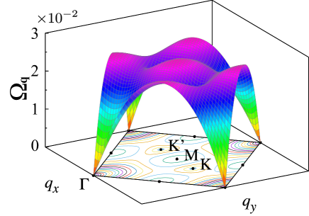
Figure 19: (color online) The FM spin wave dispersion for the effective spin Hamiltonian ${\cal H}_{\rm RKKY}$ obtained in the linear spin wave approximation at zero temperature. Here $J_{\mathrm{K}}$ is set to be one as the energy unit. The black dots in the $\Omega_{\bm{q}}=0$ plane indicate high symmetric momenta such as $\Gamma$, $M$, $K$, and $K^{\prime}$ [see Fig. 2(b)].

The linear dispersion around $\Gamma$ point implies that the contribution from the thermal excitations of the spin wave is convergent even in two spatial dimensions. More explicitly, the magnetization $m(T)$ at temperature $T$ is evaluated as

$$m(T) = m(0)-\Delta m(T),$$ (108)

where

$$\Delta m(T)=\frac{1}{N_{a}}\sum_{\mathbf{q}}\frac{1}{e^{\beta\Omega_{\mathbf{q}}}-1}$$ (109)

$$\sim \frac{1}{V_{\mathrm{BZ}}}\int_{0}^{2\pi}\mathrm{d}\theta\int_{0}^{\infty}\frac{q\mathrm{d}q}{e^{\beta cq}-1}=\frac{2\pi\zeta(2)}{V_{\mathrm{BZ}}}\frac{T^{2}}{c^{2}}$$

with $\zeta(2)=\pi^{2}/6$ (the Riemann zeta function). Here, $m(0)=1/2$ is the magnetic moment for the fully polarized FM state at $T=0$ and the long wavelength approximation of the linear dispersion relation, i.e., $\Omega_{\mathbf{q}}\simeq c|{\mathbf{q}}|$, for the spin wave dispersion is used. It is thus tempting to conclude that the critical temperature $T_{\rm C}$ for the FM order is finite even in two dimensions and is proportional to the magnon velocity $c$.

However, it should be reminded that the RKKY interaction $J_{\mathbf{R}}$ in Eq. (97) itself is temperature dependent and the temperature dependence of $J_{\mathbf{R}}$ has to be considered explicitly when the spin wave dispersion is calculated at finite temperatures. The results of the finite temperature spin wave dispersion is summarized in Fig. 20. It is clearly found in Fig. 20 that the spin wave dispersion $\Omega_{\mathbf{q}}$ is quadratic ($\Omega_{\mathbf{q}}\propto|{\mathbf{q}}|^{2}$) in the long wavelength limit around $\Gamma$ point at finite temperatures . It is now readily shown that the $q$ integral in $\Delta m(T)$ given in Eq. (109) is proportional to $\zeta(1)$, which is divergent. Therefore, we can conclude that a finite temperature FM transition is impossible and $T_{\rm C}$ should be zero.

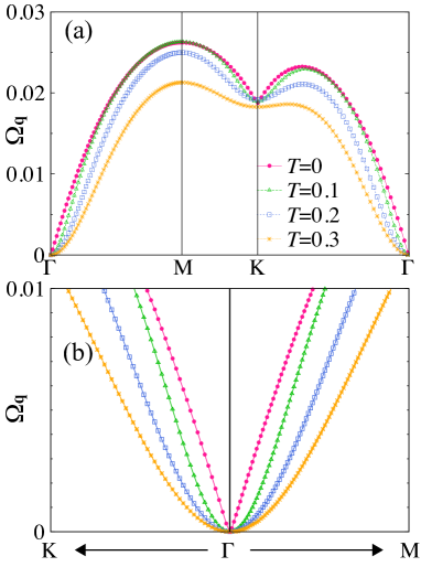
Figure 20: (color online) (a) Temperature dependence of the FM spin wave dispersion $\Omega_{\mathbf{q}}$ for the effective spin Hamiltonian ${\cal H}_{\rm RKKY}$ obtained in the linear spin wave approximation. Here the temperature dependence of the RKKY interaction $J_{\mathbf{R}}$ in Eq. (97) is explicitly considered. (b) Same as (a) but the enlarged scale at the vicinity of $\Gamma$ point near zero energy. The region of momenta taken in the horizontal axis is $0.5\pi$ in the $\Gamma$-$M$ ($\Gamma$-$K$) direction from $\Gamma$. Temperatures are indicated in (a) and $J_{\rm K}$ is set to be one as the energy unit.

A.3 Summary and remark on the FM state

Let us summarize the liner spin wave analysis for the effective spin Hamiltonian ${\cal H}_{\rm RKKY}$ and make a remark on the finite FM transition temperature $T_{\rm C}$ obtained by the VCA for the periodic Anderson model $\mathcal{H}$ in Sec. III.1. Since the RKKY interaction is FM and long-ranged, i.e., $J_{\mathbf{R}}\propto|\mathbf{R}|^{-3}$, at zero temperature Saremi2007 , the ground state of ${\cal H}_{\rm RKKY}$ is FM and the spin wave dispersion in the long wavelength limit is linear ($\sim|{\mathbf{q}}|$). However, this long range character of the RKKY interaction is true only at zero temperature and one can readily show that the RKKY interaction becomes short-ranged at finite temperatures. The resulting spin wave dispersion at finite temperatures is quadratic in the long wavelength limit ($\sim|\mathbf{q}|^{2}$), and therefore $T_{\rm C}$ should be zero. After all, the model studied here, the periodic Anderson model, only includes short range interactions and thus Mermin-Wagner theorem Mermin1966 guarantees that the FM instability should occur only at zero temperature.

The finite $T_{\rm C}$ found in the VCA for the periodic Anderson model is due merely to a mean-filed like treatment of the electron correlation beyond the size of clusters and should be regarded as a temperature where the short range FM correlations are developed. Indeed, we have found that $T_{\rm C}$ decreases with increasing the size of clusters (see Fig. 3). The considerably small $T_{\mathrm{C}}$ found in the VCA is due to the energy scale of the FM instability, namely, the exchange splitting, $\sim U(\langle n_{{\mathbf{r}}_{i}\uparrow H}\rangle-\langle n_{{\mathbf{r}}_{i}\downarrow H}\rangle)$, for small $U$ and the RKKY interaction, $\sim t_{sp}^{4}/U^{2}\times$ (static spin susceptibility of the conduction band), for large $U$.

Appendix B Application of Lieb’s theorem

In this Appendix, we consider a Hubbard model $\mathcal{H}_{\rm HM}$ described by the same Hamiltonian for the half-depleted periodic Anderson model $\mathcal{H}$ studied in the main text except that now the on-site Coulomb repulsion $U_{C}$ on the carbon conduction sites is incorporated, i.e.,

$$\mathcal{H}_{\rm HM} = -t\sum_{i,{\mathbf{\delta}},\sigma}\left(c_{{\mathbf{r}}_{i}\sigma A}^{\dagger}c_{{\mathbf{r}}_{i}+{\mathbf{\delta}}\sigma B}+{\rm H.c.}\right)$$ (110)

$$+ t_{sp}\sum_{i,\sigma}\left(c_{{\mathbf{r}}_{i}\sigma B}^{\dagger}c_{{\mathbf{r}}_{i}\sigma H}+{\rm H.c.}\right)$$

$$+ U\sum_{i}\left(n_{{\mathbf{r}}_{i}\uparrow H}-\frac{1}{2}\right)\left(n_{{\mathbf{r}}_{i}\downarrow H}-\frac{1}{2}\right)$$

$$+ U_{C}\sum_{i,\alpha=A,B}\left(n_{{\mathbf{r}}_{i}\uparrow\alpha}-\frac{1}{2}\right)\left(n_{{\mathbf{r}}_{i}\downarrow\alpha}-\frac{1}{2}\right)$$

defined on the lattice shown in Fig. 1. In the following, we analyze the ground state of this Hubbard model $\mathcal{H}_{\rm HM}$ at half filling based on Lieb’s theorem on a bipartite lattice Lieb .

Following Lieb’s argument in Ref. Lieb , we can show that the ground state of $\mathcal{H}_{\rm HM}$ has the following properties: (a) among the possibly degenerate ground states, there exists one state which has total spin $S=0$, when $U\leq 0$ and $U_{C}\leq 0$ and (b) the ground state is unique if $U<0$ and $U_{C}<0$. The details of the proof are found in Ref. Lieb . Here, we only note that in the proof the matrix $L_{{\mathbf{r}}_{i}}=\left<\bar{\alpha}\right|n_{{\mathbf{r}}_{i}\sigma}\left|\bar{\beta}\right>$ defined in Ref. Lieb should be replaced by $\left<\bar{\alpha}\right|(n_{{\mathbf{r}}_{i}\sigma\alpha}-1/2)\left|\bar{\beta}\right>$, where $\left|\bar{\alpha}\right>$ and $\left|\bar{\beta}\right>$ represent sets of real space configurations of electrons with spin $\sigma$.

Let us now map the Hubbard model $\mathcal{H}_{\rm HM}$ onto a negative $U$ Hubbard model by the particle-hole transformation

$$\bar{c}_{{\mathbf{r}}_{i}\uparrow H} = c_{{\mathbf{r}}_{i}\uparrow H},\quad\bar{c}_{{\mathbf{r}}_{i}\downarrow H}=c^{\dagger}_{{\mathbf{r}}_{i}\downarrow H},$$

$$\bar{c}_{{\mathbf{r}}_{i}\uparrow A} = c_{{\mathbf{r}}_{i}\uparrow A},\quad\bar{c}_{{\mathbf{r}}_{i}\downarrow A}=c^{\dagger}_{{\mathbf{r}}_{i}\downarrow A},$$

$$\bar{c}_{{\mathbf{r}}_{i}\uparrow B} = c_{{\mathbf{r}}_{i}\uparrow B},\quad\bar{c}_{{\mathbf{r}}_{i}\downarrow B}=-c^{\dagger}_{{\mathbf{r}}_{i}\downarrow B}.$$ (111)

With this transformation, the Hubbard model ${\mathcal{H}}_{\rm HM}$ is mapped onto

$$\bar{\mathcal{H}}_{\rm HM} = -t\sum_{i,{\mathbf{\delta}},\sigma}\left(\bar{c}_{{\mathbf{r}}_{i}\sigma A}^{\dagger}\bar{c}_{{\mathbf{r}}_{i}+{\mathbf{\delta}}\sigma B}+{\rm H.c.}\right)$$ (112)

$$+ t_{sp}\sum_{i,\sigma}\left(\bar{c}_{{\mathbf{r}}_{i}\sigma B}^{\dagger}\bar{c}_{{\mathbf{r}}_{i}\sigma H}+{\rm H.c.}\right)$$

$$- U\sum_{i}\left(\bar{n}_{{\mathbf{r}}_{i}\uparrow H}-\frac{1}{2}\right)\left(\bar{n}_{{\mathbf{r}}_{i}\downarrow H}-\frac{1}{2}\right)$$

$$- U_{C}\sum_{i,\alpha=A,B}\left(\bar{n}_{{\mathbf{r}}_{i}\uparrow\alpha}-\frac{1}{2}\right)\left(\bar{n}_{{\mathbf{r}}_{i}\downarrow\alpha}-\frac{1}{2}\right),$$

where $\bar{n}_{{\mathbf{r}}_{i}\sigma\alpha}=\bar{c}^{\dagger}_{{\mathbf{r}}_{i}\sigma\alpha}\bar{c}_{{\mathbf{r}}_{i}\sigma\alpha}$.

Applying Lieb’s theorem to the negative $U$ Hubbard model ${\bar{\mathcal{H}}}_{\rm HM}$, we can readily show that (i) the ground state of ${\mathcal{H}}_{\rm HM}$ at half filling is unique (apart from the trivial spin degeneracy) and it has total spin $S=\left(|H|+|A|-|B|\right)/2$ when $U>0$ and $U_{C}>0$ and (ii) one of the possibly degenerate ground states of ${\mathcal{H}}$ (i.e., ${\mathcal{H}}_{\rm HM}$ with $U_{C}=0$) at half filling has total spin $S=\left(|H|+|A|-|B|\right)/2$ when $U>0$.

To prove statement (i), we should first notice that the corresponding spin-1/2 Heisenberg model obtained in the limit of $U$, $U_{C}\to\infty$ is defined on the bipartite lattice and thus Lieb-Mattis theorem guarantees the unique ground state of this spin-1/2 Heisenberg model with total spin $S=\left(|H|+|A|-|B|\right)/2$ LM . Applying Lieb’s theorem (b) to ${\bar{\mathcal{H}}}_{\rm HM}$ for $U>0$ and $U_{C}>0$, we can now show that the ground state of ${\mathcal{H}}_{\rm HM}$ is unique, apart from the trivial degeneracy due to the spin rotational symmetry, for any finite value of $U_{C}$ until $U_{C}\to 0^{+}$ and the total spin of the ground state is $S=\left(|H|+|A|-|B|\right)/2$ note10 .

When $U_{C}$ is exactly zero, the uniqueness of the ground state of ${\mathcal{H}}_{\rm HM}$ is no longer guaranteed. However, according to Lieb’s theorem (a), the state with $S=\left(|H|+|A|-|B|\right)/2$ must be the ground state or one of the possibly degenerate ground states, which thus proves statement (ii). In the next Appendix, we will show by numerically exactly diagonalizing small clusters that indeed the ground state of ${\mathcal{H}}$ is unique and it has total spin $S=\left(|H|+|A|-|B|\right)/2$ when $U>0$.

Appendix C Numerically exact diagonalization study of the ground state phase diagram

Although Lieb’s theorem does not guarantee the unique ground state of ${\mathcal{H}}$ at half filling, here we perform numerically exact diagonalization calculations for small clusters to show that the ground state of ${\mathcal{H}}_{\rm HM}$ at half filling for $U,\,U_{C}>0$ is smoothly connected to the one even for $U_{C}$ approaching exactly to zero, namely, the ground state of ${\mathcal{H}}$ at half filling is unique with its total spin $S=\left(|H|+|A|-|B|\right)/2$.

Figure 21 shows the ground state phase diagrams for ${\mathcal{H}}_{\rm HM}$ at hall filling obtained by numerically exactly diagonalizing the 12-site cluster (see Fig. 1) with periodic and open boundary conditions. We find for both boundary conditions that the ground state for $U>0$ and $U_{C}>0$ is indeed unique and it has total spin $S=\left(|H|+|A|-|B|\right)/2$, in good accordance with Lieb’s theorem. We also find in Fig. 21 that the ground state for $U>0$ and $U_{C}>0$ is smoothly connected to the unique ground state for $U_{C}=0$, where Lieb’s theorem does not guarantee the uniqueness of the ground state. Therefore, we conclude that the ground state of ${\mathcal{H}}$ at half filling is unique and it has total spin $S=\left(|H|+|A|-|B|\right)/2$ as long as $U>0$. This also proves that the FM ground state of ${\mathcal{H}}$ found in the main text is smoothly connected to the Lieb-Mattis type ferromagnetism.

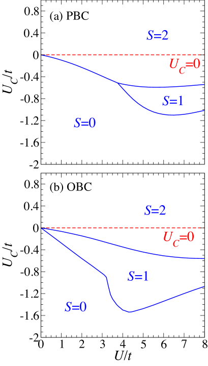
Figure 21: (color online) The ground state phase diagrams of ${\mathcal{H}}_{\rm HM}$ for $t_{sp}=t$ at half filling. The results are obtained by numerically exactly diagonalizing the 12-site clusters, containing 4 unit cells (see Fig 1), with (a) periodic boundary conditions (PBC) and (b) open boundary conditions (OBC). The total spin $S$ of the ground state is indicated in the figures. The ground state with $S=2$ is found all unique. ${\mathcal{H}}_{\rm HM}$ with $U_{C}=0$ (indicated by red dashed lines) corresponds to the periodic Anderson model $\mathcal{H}$ studied in the min text.

Appendix D Single-particle excitations in the Hubbard-I approximation

The analytical forms of the single-particle excitation dispersion $\omega_{\nu,\mathbf{k}}$ and the corresponding spectral weight $\boldsymbol{\rho}_{\nu,\mathbf{k}}$ obtained by the Hubbard-I approximation are provided in Eq. (29) and Eqs. (38) and (39), respectively. Here, in this Appendix, we shall examine these quantities for several limiting cases.

D.1 Noninteracting limit

In the noninteracting limit, the energy dispersions are given as

$$\lim_{U\rightarrow 0}\omega_{1/4,\mathbf{k}} = \pm\sqrt{|\gamma_{\mathbf{k}}|^{2}+t_{sp}^{2}},$$ (113)

$$\lim_{U\rightarrow 0}\omega_{2/3,\mathbf{k}} = 0,$$ (114)

and the spectral weights are given as

$$\lim_{U\rightarrow 0}\boldsymbol{\rho}_{1/4,\mathbf{k}} = \frac{1}{2(|\gamma_{\mathbf{k}}|^{2}+t_{sp}^{2})}\left(\begin{array}[]{ccc}|\gamma_{\mathbf{k}}|^{2}&\pm\gamma_{\mathbf{k}}\sqrt{|\gamma_{\mathbf{k}}|^{2}+t_{sp}^{2}}&t_{sp}\gamma_{\mathbf{k}}\\ \pm\gamma_{\mathbf{k}}^{*}\sqrt{|\gamma_{\mathbf{k}}|^{2}+t_{sp}^{2}}&|\gamma_{\mathbf{k}}|^{2}+t_{sp}^{2}&\pm t_{sp}\sqrt{|\gamma_{\mathbf{k}}|^{2}+t_{sp}^{2}}\\ t_{sp}\gamma_{\mathbf{k}}^{*}&\pm t_{sp}\sqrt{|\gamma_{\mathbf{k}}|^{2}+t_{sp}^{2}}&t_{sp}^{2}\end{array}\right),$$ (118)

$$\lim_{U\rightarrow 0}\boldsymbol{\rho}_{2/3,\mathbf{k}} = \frac{-1}{2(|\gamma_{\mathbf{k}}|^{2}+t_{sp}^{2})}\left(\begin{array}[]{ccc}-t_{sp}^{2}&0&t_{sp}\gamma_{\mathbf{k}}\\ 0&0&0\\ t_{sp}\gamma_{\mathbf{k}}^{*}&0&-|\gamma_{\mathbf{k}}|^{2}\end{array}\right).$$ (122)

These results are also obtained directly by solving the noninteracting Hamiltonian ${\mathcal{H}}_{0}$. It is apparent in Eqs. (114) and (122) that the flat band, corresponding to the inner two bands with $\nu=2$ and $3$, is composed solely of $A$ and $H$ orbitals, but not $B$ orbital, i.e., $B$ orbital being completely decoupled from the flat band (see the top panels of Fig. 16).

D.2 Localized spin limit

A single electron is localized on each hydrogen impurity site when $U$ is large enough, and eventually the hydrogen impurity sites are decoupled from the conduction band in the limit of $U\to\infty$. In this limit, the energy dispersions are given as

$$\lim_{U\rightarrow\infty}\omega_{1/4,\mathbf{k}} \simeq \pm\lim_{U\rightarrow\infty}\frac{U}{2},$$ (123)

$$\lim_{U\rightarrow\infty}\omega_{2/3,\mathbf{k}} = \pm|\gamma_{\mathbf{k}}|,$$ (124)

and the corresponding spectral weights are

$$\lim_{U\rightarrow\infty}\boldsymbol{\rho}_{1/4,\mathbf{k}} = \frac{1}{2}\left(\begin{array}[]{ccc}0&0&0\\ 0&0&0\\ 0&0&1\end{array}\right),$$ (128)

$$\lim_{U\rightarrow\infty}\boldsymbol{\rho}_{2/3,\mathbf{k}} = \frac{1}{2}\left(\begin{array}[]{ccc}1&\pm\frac{\gamma_{\mathbf{k}}}{|\gamma_{\mathbf{k}}|}&0\\ \pm\frac{\gamma_{\mathbf{k}}^{*}}{|\gamma_{\mathbf{k}}|}&1&0\\ 0&0&0\end{array}\right).$$ (132)

Thus, as expected, the hydrogen impurity sites are completely detached from the carbon conduction sites, forming the upper and lower Hubbard band in the atomic limit, which correspond to the outer two bands with $\nu=1$ and $4$, respectively. The inner two bands with $\nu=2$ and $3$ simply display the energy dispersion of the conduction band, i.e., the massless Dirac dispersion for the pure graphene model.

D.3 Decoupling limit

If $t_{sp}$ is zero, the hydrogen impurity sites are decoupled from the conduction band. In this limit, the energy dispersions are give as

$$\lim_{t_{sp}\rightarrow 0}\omega_{1/4,\mathbf{k}} = \pm\frac{U}{2},$$ (133)

$$\lim_{t_{sp}\rightarrow 0}\omega_{2/3,\mathbf{k}} = \pm|\gamma_{\mathbf{k}}|,$$ (134)

and the spectral weights are given as

$$\lim_{t_{sp}\rightarrow 0}\boldsymbol{\rho}_{1/4,\mathbf{k}} = \frac{1}{2}\left(\begin{array}[]{ccc}0&0&0\\ 0&0&0\\ 0&0&1\end{array}\right),$$ (138)

$$\lim_{t_{sp}\rightarrow 0}\boldsymbol{\rho}_{2/3,\mathbf{k}} = \frac{1}{2}\left(\begin{array}[]{ccc}1&\pm\frac{\gamma_{\mathbf{k}}}{|\gamma_{\mathbf{k}}|}&0\\ \pm\frac{\gamma_{\mathbf{k}}^{*}}{|\gamma_{\mathbf{k}}|}&1&0\\ 0&0&0\end{array}\right).$$ (142)

It is interesting to notice that these are exactly the same as those in the limit of $U\to\infty$.

D.4 Strong bonding limit

If $|t_{sp}|$ is large, it is expected that the bonding and anti-bonding “molecular” orbitals are formed locally between the neighboring $B$ and $H$ orbitals, and as a result $A$ orbital is isolated. In this limit, the energy dispersions are given as

$$\lim_{|t_{sp}|\rightarrow\infty}\omega_{1/4,\mathbf{k}} \simeq \pm\lim_{|t_{sp}|\rightarrow\infty}|t_{sp}|$$ (143)

$$\lim_{|t_{sp}|\rightarrow\infty}\omega_{2/3,\mathbf{k}} = 0,$$ (144)

and the spectral weights are given as

$$\lim_{|t_{sp}|\rightarrow\infty}\boldsymbol{\rho}_{1/4,\mathbf{k}} = \frac{1}{2}\left(\begin{array}[]{ccc}0&0&0\\ 0&1&\pm\frac{t_{sp}}{|t_{sp}|}\\ 0&\pm\frac{t_{sp}}{|t_{sp}|}&1\end{array}\right),$$ (148)

$$\lim_{|t_{sp}|\rightarrow\infty}\boldsymbol{\rho}_{2/3,\mathbf{k}} = \frac{1}{2}\left(\begin{array}[]{ccc}1&0&0\\ 0&0&0\\ 0&0&0\end{array}\right).$$ (152)

It is apparent from these results that $B$ and $H$ orbitals are indeed tightly bound to form the bonding and anti-bonding “molecular” orbitals and the isolated $A$ orbitals are completely localized.

Appendix E Brillouin-Wigner perturbation theory for the quasiparticle Hamiltonian $\mathcal{H}_{\text{H-I}}$

In this Appendix, we apply the Brillouin-Wigner (BW) perturbation theory BW to the quasiparticle Hamiltonian $\mathcal{H}_{\text{H-I}}$ in Eq. (61) and derive effective Hamiltonians for the Dirac band as well as for the upper and lower Hubbard bands.

E.1 BW perturbation theory

Let us first divide the $4\times 4$ quasiparticle Hamiltonian matrix $\boldsymbol{H}$, defining the quasiparticle Hamiltonian $\mathcal{H}_{\text{H-I}}$ in Eq. (61), into $2\times 2$ submatrices, i.e.,

$$\boldsymbol{H} = \left(\begin{array}[]{cc|cc}0&\gamma_{\mathbf{k}}&0&0\\ \gamma^{*}_{\mathbf{k}}&0&t_{sp}&0\\ \hline\cr 0&t_{sp}&0&U/2\\ 0&0&U/2&0\end{array}\right)$$ (157)

$$= \left(\begin{array}[]{c|c}\boldsymbol{A}&\boldsymbol{B}\\ \hline\cr\boldsymbol{C}&\boldsymbol{D}\end{array}\right),$$ (160)

where $\boldsymbol{A}$, $\boldsymbol{B}$, $\boldsymbol{C}$, and $\boldsymbol{D}$ are the corresponding $2\times 2$ matrices. Then, applying the BW perturbation theory, i.e., the energy dependent perturbation theory, the energy ($\omega$) dependent effective Hamiltonian matrix $\boldsymbol{H}_{\rm eff}(\omega)$ is given as

$$\boldsymbol{H}_{\rm eff}(\omega) = \boldsymbol{P}\boldsymbol{H}\sum_{n=0}^{\infty}\left[\boldsymbol{Q}\left(\omega-\boldsymbol{H}_{0}\right)^{-1}\boldsymbol{H_{1}}\right]^{n}$$ (161)

$$= \boldsymbol{P}\boldsymbol{H}+\boldsymbol{P}\boldsymbol{H}\boldsymbol{Q}\left(\omega-\boldsymbol{H}_{0}\right)^{-1}\boldsymbol{H_{1}}+\cdots,$$

where

$$\boldsymbol{H}_{0}=\left(\begin{array}[]{c|c}\boldsymbol{A}&\boldsymbol{0}\\ \hline\cr\boldsymbol{0}&\boldsymbol{D}\end{array}\right)$$ (162)

is the unperturbed part and

$$\boldsymbol{H_{1}}=\left(\begin{array}[]{c|c}\boldsymbol{0}&\boldsymbol{B}\\ \hline\cr\boldsymbol{C}&\boldsymbol{0}\end{array}\right)$$ (163)

is the perturbation. Here, $\boldsymbol{0}$ represents the $2\times 2$ null matrix. $\boldsymbol{P}$ and $\boldsymbol{Q}$ are the projection matrices onto the target (i.e., effective model) space and the space orthogonal to the target space, respectively, and they satisfy that $\boldsymbol{P}^{2}=\boldsymbol{P}$ and $\boldsymbol{P}+\boldsymbol{Q}=\boldsymbol{I}$, which lead to $\boldsymbol{Q}^{2}=\boldsymbol{Q}$ and $\boldsymbol{PQ}=\boldsymbol{0}$.

E.2 Effective Hamiltonian for the Dirac band

To obtain an effective Hamiltonian projected onto the carbon conduction sites, the projection matrices should be

$$\boldsymbol{P}={\rm diag}(1,1,0,0)$$ (164)

and

$$\boldsymbol{Q}={\rm diag}(0,0,1,1).$$ (165)

Then the effective Hamiltonian is given as

$$\boldsymbol{P}(\omega-\boldsymbol{H}_{\rm eff}(\omega))\boldsymbol{P}=\left(\begin{array}[]{c|c}\boldsymbol{g}_{\rm eff,Gr}^{-1}(\omega)&\boldsymbol{0}\\ \hline\cr\boldsymbol{0}&\boldsymbol{0}\end{array}\right),$$ (166)

where, up to the second order of $t_{sp}$, we obtain that

$$\boldsymbol{g}_{\rm eff,Gr}^{-1}(\omega) = (\omega-\boldsymbol{A})-\boldsymbol{B}\left(\omega-\boldsymbol{D}\right)^{-1}\boldsymbol{C}$$ (171)

$$= \left(\begin{array}[]{cc}\omega&-\gamma\\ -\gamma^{*}&\omega\end{array}\right)-\left(\begin{array}[]{cc}0&0\\ 0&\displaystyle\frac{t^{2}_{sp}\omega}{\omega^{2}-(U/2)^{2}}\end{array}\right)$$

$$= \left(\begin{array}[]{cc}\omega&-\gamma_{\mathbf{k}}\\ -\gamma_{\mathbf{k}}^{*}&\omega\displaystyle-\frac{t^{2}_{sp}\omega}{\omega^{2}-(U/2)^{2}}\end{array}\right).$$ (174)

Notice that this is a Schur’s complement of $\omega-\boldsymbol{H}$ with respect to $\omega-\boldsymbol{D}$. The effective Hamiltonian $\boldsymbol{h}_{\rm eff,Gr}(\omega)$ of the target space is thus obtained as

$$\boldsymbol{h}_{\rm eff,Gr}(\omega): = \omega-\boldsymbol{g}_{\rm eff,Gr}^{-1}(\omega)$$ (177)

$$= \left(\begin{array}[]{cc}0&\gamma_{\mathbf{k}}\\ \gamma_{\mathbf{k}}^{*}&\displaystyle\frac{t^{2}_{sp}\omega}{\omega^{2}-(U/2)^{2}}\end{array}\right).$$

From Eq. (177), we find that (i) when $\omega\to 0$ and $|U|>0$, the effective Hamiltonian is the same as the pure graphene model, and (ii) when $U=0$, the effective on-site energy of $B$ orbital diverges in the limit of $\omega\to 0$, implying that $B$ orbital does not involve the flat band formation.

The eigenvalue problem of the target space in the BW perturbation theory is described as

$$\boldsymbol{h}_{\rm eff,Gr}(\omega)\boldsymbol{\psi}_{\rm eff,Gr}=\omega\boldsymbol{\psi}_{\rm eff,Gr},$$ (178)

where $\boldsymbol{\psi}_{\rm eff,Gr}$ is the two dimensional eigenstate vector and the eigenvalues are given as the roots of the secular equation

$$\det\left[\omega-\boldsymbol{h}_{\rm eff,Gr}(\omega)\right]=\det\boldsymbol{g}_{\rm eff,Gr}^{-1}(\omega)=0.$$ (179)

Noticing that the determinant formula for the block matrix

$$\det\boldsymbol{H}=\det\boldsymbol{D}\cdot\det(\boldsymbol{A}-\boldsymbol{B}\boldsymbol{D}^{-1}\boldsymbol{C}),$$ (180)

we find that the eigenvalues are given as the roots of

$$\det\boldsymbol{g}_{\rm eff,Gr}^{-1}(\omega)=\frac{\det(\omega-\boldsymbol{H})}{\det(\omega-\boldsymbol{D})}=0.$$ (181)

Therefore, the eigenvalues are identical to those obtained by the full eigenvalue problem of $\boldsymbol{H}$, i.e.,

$$\omega=\pm\omega_{+,\mathbf{k}},\ {\rm and}\ \pm\omega_{-,\mathbf{k}}$$ (182)

in Eq. (29).

We have obtained the exact eigenvalues from the effective Hamiltonian which is derived perturbatively only up to ${\mathcal{O}}(t_{sp}^{2})$. This is because the eigenvalues of the full Hamiltonian are determined by the roots of $\det(\omega-\boldsymbol{H})=\det(\omega-\boldsymbol{D})\cdot\det\left[\boldsymbol{A}-\boldsymbol{B}(\omega-\boldsymbol{D})^{-1}\boldsymbol{C})\right]=0$, which contains the term $\boldsymbol{B}(\omega-\boldsymbol{D})^{-1}\boldsymbol{C}$, equivalent to the second order perturbation with respect to $t_{sp}$.

E.3 Effective Hamiltonian for the upper and lower Hubbard bands

An effective Hamiltonian projected onto the upper and lower Hubbard bands is obtained by considering the projection matrices

$$\boldsymbol{P}={\rm diag}(0,0,1,1)$$ (183)

and

$$\boldsymbol{Q}={\rm diag}(1,1,0,0).$$ (184)

The effective Hamiltonian is then given as

$$\boldsymbol{P}(\omega-\boldsymbol{H}_{\rm eff}(\omega))\boldsymbol{P}=\left(\begin{array}[]{c|c}\boldsymbol{0}&\boldsymbol{0}\\ \hline\cr\boldsymbol{0}&\boldsymbol{g}_{\rm eff,Hub}^{-1}(\omega)\\ \end{array}\right),$$ (185)

where, up to $t_{sp}^{2}$, we obtain that

$$\boldsymbol{g}_{\rm eff,Hub}^{-1}(\omega) = (\omega-\boldsymbol{D})-\boldsymbol{C}\left(\omega-\boldsymbol{A}\right)^{-1}\boldsymbol{B}$$ (190)

$$= \left(\begin{array}[]{cc}\omega&-U/2\\ -U/2&\omega\end{array}\right)-\left(\begin{array}[]{cc}\displaystyle\frac{t^{2}_{sp}\omega}{\omega^{2}-|\gamma_{\mathbf{k}}|^{2}}&0\\ 0&0\end{array}\right)$$

$$= \left(\begin{array}[]{cc}\omega-\displaystyle\frac{t^{2}_{sp}\omega}{\omega^{2}-|\gamma_{\mathbf{k}}|^{2}}&-U/2\\ -U/2&\omega\end{array}\right).$$ (193)

Notice that this is a Schur’s complement of $\omega-\boldsymbol{H}$ with respect to $\omega-\boldsymbol{A}$. The effective Hamiltonian $\boldsymbol{h}_{\rm eff,Hub}(\omega)$ is therefore obtained as

$$\boldsymbol{h}_{\rm eff,Hub}(\omega): = \omega-\boldsymbol{g}_{\rm eff,Hub}^{-1}(\omega)$$ (196)

$$= \left(\begin{array}[]{cc}\displaystyle\frac{t^{2}_{sp}\omega}{\omega^{2}-|\gamma_{\mathbf{k}}|^{2}}&U/2\\ U/2&0\end{array}\right).$$

From Eq. (196) we find that (i) when $\omega\to 0$ and at momentum $\mathbf{k}$ away from $K$ and $K^{\prime}$ points, the effective model simply describes the upper and lower Hubbard bands in the atomic limit, (ii) when $\omega\to 0$ and at $\mathbf{k}=K(K^{\prime})$, the effective on-site energy of $H$ orbital diverges, indicating that the contribution of $H$ orbital is absent at $K(K^{\prime})$ in the Dirac band, and (iii) when $\omega\to\pm|\gamma_{\mathbf{k}}|$, the effective on-site energy of $H$ orbital diverges, which is consistent with the “dark spectral” region found in both CPT and Hubbard-I approximation. Finally, we note that the eigenvalues of $\boldsymbol{h}_{\rm eff,Hub}(\omega)$ are also identical to the ones obtained by the full eigenvalue problem of $\boldsymbol{H}$.

References

- (1) K. S. Novoselov, A. K. Geim, S. V. Morozov, D. Jiang, M. I. Katsnelson, I. V. Grigorieva, S. V. Dubonos, and A. A. Firsov, Nature, 438, 197 (2005).
- (2) A. H. Castro Neto, F. Guinea, N. M. R. Peres, K. S. Novoselov, and A. K. Geim, Rev. Mod. Phys. 81, 109 (2009).
- (3) P. R. Wallace, Phys. Rev. 71, 622 (1947).
- (4) V. N. Kotov, B. Uchoa, V. M. Pereira, F. Guinea, and A. H. Castro Neto, Rev. Mod. Phys. 84, 1067 (2012).
- (5) Z. Y. Meng, T. C. Lang, S. Wessel, F. F. Assaad, and A. Muramatsu, Nature 464, 847–851 (2010).
- (6) S. Sorella, Y. Otsuka, and S. Yunoki, Sci. Rep. 2, 992 (2012).
- (7) F. F. Assaad and I. F. Herbut, Phys. Rev. X 3, 031010 (2013).
- (8) F. Parisen Toldin, M. Hohenadler, F. F. Assaad, and I. F. Herbut, Phys. Rev. B 91, 165108 (2015).
- (9) Y. Otsuka, S. Yunoki, and S. Sorella, e-print, arXiv:1510.08593.
- (10) J. O. Sofo, A. S. Chaudhari, and G. D. Barber, Phys. Rev. B 75, 153401 (2007).
- (11) D. C. Elias, R. R. Nair, T. M. G. Mohiuddin, S. V. Morozov, P. Blake, M. P. Halsall, A. C. Ferrari, D. W. Boukhvalov, M. I. Katsnelson, A. K. Geim, and K. S. Novoselov, Science 323, 610 (2009).
- (12) S. C. Ray, N. Soin, T. Makgato, C. H. Chuang, W. F. Pong, S. S. Roy, S. K. Ghosh, A. M. Strydom, and J. A. McLaughlin, Sci. Rep. 4, 3862 (2014).
- (13) Q. Peng, A. K. Dearden, J. Crean, L. Han, S. Liu, X. Wen, and S. De, Nan., Sci. and Appl. 7, 1 (2014).
- (14) J. Zhou, Q. Wang, Q. Sun, X. S. Chen, Y. Kawazoe, and P. Jena, Nano Lett., 9 3867 (2009).
- (15) A. N. Rudenko, F. J. Keil, M. I. Katsnelson, and A. I. Lichtenstein, Phys. Rev. B 88 081405(R) (2013).
- (16) A. H. Castro Neto, and F. Guinea, Phys. Rev. Lett. 103, 026804 (2009).
- (17) M. Gmitra, D. Kochan, and J. Fabian, Phys. Rev. Lett. 110, 246602 (2013).
- (18) M. Schuler, M. Rosner, T. O. Wehling, A. I. Lichtenstein, and M. I. Katsnelson, Phys. Rev. Lett. 111, 036601 (2013).
- (19) S. Sorella and E. Tosatti, Europhys. Lett. 19, 699 (1992).
- (20) P. Fulde, Correlated Electrons in Quantum Matter (World Scientific, 2012), Chap. 1 and Chap. 10.
- (21) R. Eder, H. F. Pen, and G. A. Sawatzky, Phys. Rev. B 56, 10115 (1997).
- (22) M. Potthoff, M. Aichhorn, and C. Dahnken, Phys. Rev. Lett. 91, 206402 (2003).
- (23) D. Sénéchal, D. Perez, and M. Pioro-Ladrière, Phys. Rev. Lett. 84, 522 (2000).
- (24) E. H. Lieb, Phys. Rev. Lett. 62, 1201 (1989).
- (25) S. Horiuchi, S. Kudo, T. Shirakawa, and Y. Ohta, Phys. Rev. B 78, 155128 (2008).
- (26) K. Seki, T. Shirakawa, Q. Zhang, T. Li, and S. Yunoki, J. Phys: Conf. Ser. 603, 012024 (2015).
- (27) A similar model on the square lattice has been studied by I. Titvinidze, A. Schwabe, and M. Potthoff in Phys. Rev. B 90, 045112 (2014).
- (28) M. A. Ruderman and C. Kittel, Phys. Rev. 96, 99 (1954); T. Kasuya, Prog. Theor. Phys. 16, 45 (1956); K. Yoshida, Phys. Rev. 106, 893 (1958).
- (29) S. Saremi, Phys. Rev. B, 76, 184430 (2007).
- (30) E. H. Lieb and D. Mattis, J. Math. Phys. 3, 749 (1962).
- (31) N. Mermin and H. Wagner, Phys. Rev. Lett. 17, 1133 (1966).
- (32) J. Hubbard, Proc. Roy. Soc. London A 276, 238 (1963).
- (33) Y. Hatsugai, T. Fukui, and H. Aoki, Eur. Phys. J. Specical Topics 148, 133 (2007).
- (34) Y. Hatsugai, T. Morimoto, T. Kawarabayashi, Y. Hamamoto, and H. Aoki, New. J. Phys. 15, 035023 (2013).
- (35) Y. Hatsugai and H. Aoki, Graphene: Topological proerties, Chiral Symmetry, and Their Manipulation. in Physics of Graphene eds. H. Aoki and M. S. Dresselhause, (Springer, 2014), Chap. 7.
- (36) B. A. Bernevig and T. L. Hughes, Topological Insulators and Topological Superconductors (Princeton University press, 2013) Chap. 7.
- (37) S. Sakai, M. Civelli, and M. Imada, e-print, arXiv:1411.4365.
- (38) H. Ishizuka and Y. Motome, Phys. Rev. Lett. 109, 237207 (2012).
- (39) C.-H. Lin and W. Ku, e-print, arXiv:1303.4822.
- (40) A. Varykhalov, D. Marchenko, J. Sanchez-Barriga, M. R. Scholz, B. Verberck, B. Trauzettel, T. O. Wehling, C. Carbone, and O. Rader, Phys. Rev. X 2, 041017 (2012).
- (41) The singlet ground state of the undepleted symmetric periodic Anderson model on a bipartite lattice has been proved by K. Ueda, H. Tsunetsugu, and M. Sigrist in Phys. Rev. Lett. 68 1030 (1992).
- (42) P. Fulde, Electron Correlations in Molecules and Solids, Third Enlarged Edition, (Springer, 1995), Chap. 4.