Dark solitons in the Lugiato-Lefever equation with normal dispersion

Abstract

The regions of existence and stability of dark solitons in the Lugiato-Lefever model with normal chromatic dispersion are described. These localized states are shown to be organized in a bifurcation structure known as collapsed snaking implying the presence of a region in parameter space with a finite multiplicity of dark solitons. For some parameter values dynamical instabilities are responsible for the appearance of oscillations and temporal chaos. The importance of the results for understanding frequency comb generation in microresonators is emphasized.

I Introduction

Dark solitons, localized spots of lower intensity embedded in an homogeneous surrounding, are a particular type of solitons appearing in conservative or dissipative systems far from thermodynamic equilibrium Akhmediev . In the latter case they are known as dissipative solitons (DSs) and related structures can be found in a large variety of systems, including those found in chemistry chemist , gas discharges discharges , fluid mechanics fluid , vegetation and plant ecology vege , as well as optics spatial_CS , where they are known as cavity solitons. These structures arise as a result of a balance between nonlinearity and spatial coupling, and between driving and dissipation. In this work we focus on the field of optics, and study DSs in single mode fiber resonators and microresonators where they are known as temporal solitons leo_nat . These systems are commonly described by the Lugiato-Lefever equation (LLE), a mean field model originaly introduced in lugiato_spatial_1987 in the context of ring cavities or a Fabry-Perot interferometer with transverse spatial extent, partially filled with a nonlinear medium. In temporal systems bright and dark solitons can be found. Taking into account only second order dispersion (SOD) two regimes can be identified, characterized by either normal or anomalous chromatic dispersion. In the latter case the only type of DSs that exist are bright solitons arising in both the monostable gomila_Scroggi and bistable regimes leo-lendert ; Parra_Rivas_2 ; Goday_chembo . In contrast, in the normal SOD case the main type of DSs that appear are dark solitons Goday_chembo ; Xue_NP ; Lobanov_OE ; KFC_dark . In this work we provide a detailed analysis of the bifurcation structure and stability of dark DSs appearing in the normal dispersion regime, classifying the different dynamical regimes arising in this system.

The organization of this paper is as follows. In Sec. II, we introduce the Lugiato-Lefever model in the context of temporal dynamics in fiber resonators and microresonators. We then analyze the spatial dynamics of spatially uniform states (Sec. III), followed in Sec. IV by an analysis of the bifurcation structure of dark solitons. In Sec. V we analyze oscillatory and chaotic dynamics of dark solitons. We conclude in Sec. VI by discussing the generality of the analysis provided in the earlier sections and in particular its relevance to frequency combs in nonlinear optics.

II The Lugiato-Lefever equation

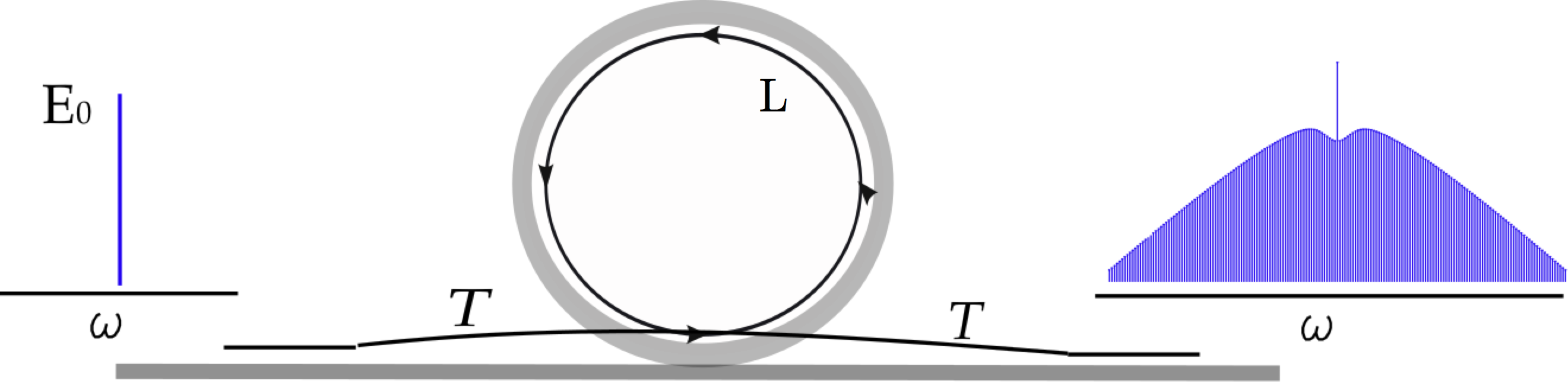
Figure 1: (Color online) A synchronously pumped fiber cavity. Here $T$ is the transmission coefficient of the beam splitter and $L$ is the length of the fiber.

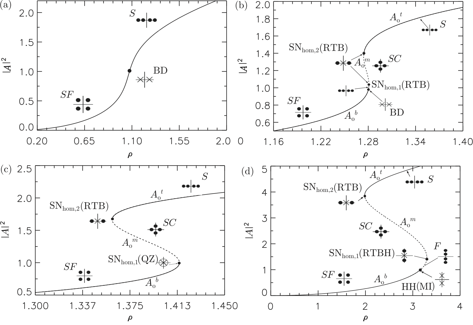
Figure 2: Spatial eigenvalues of $A_{0}$ for several values of $\theta$. (a) $\theta=1.4<\sqrt{3}$; (b) $\sqrt{3}<\theta=1.8<2$; (c) $\theta=2$; (d) $2<\theta=4$. The different labels are explained in Table 1. Solid (dashed) lines indicate stability (instability) in time.

In this section we provide a brief introduction to the LLE in the context of fiber resonators and microresonators. We then employ the normalization of leo-lendert to study the continuous wave (CW) or equivalently the homogeneous steady state (HSS) solutions of this model and to determine their temporal stability. Figure 1 shows a fiber cavity of length $L$ with a beam splitter with transmission coefficient $T$ and a continuous wave source of amplitude $E_{0}$. At the beam splitter, the pump is coupled to the electromagnetic wave circulating inside the fiber. Under these conditions the evolution of the electric field $E\equiv E(t^{\prime},\tau)$ within the cavity is described by the following evolution equation Haelterman ,

$$t_{R}\frac{\partial E}{\partial t^{\prime}}=-(\alpha+i\delta_{0})E-i\frac{L\beta_{2}}{2}\frac{\partial^{2}E}{\partial\tau^{2}}+i\gamma L|E|^{2}E+\sqrt{T}E_{0},$$ (1)

where $\alpha>0$ describes the total cavity losses, $\beta_{2}$ is the second order dispersion coefficient ($\beta_{2}>0$ in the normal dispersion case while $\beta_{2}<0$ in the anomalous case), $\gamma>0$ is a nonlinear coefficient arising from the Kerr effect in the resonator, and $\delta_{0}$ is the cavity detuning. Here $\tau$ is the fast time describing the temporal structure of the nonlinear waves while the slow time $t^{\prime}$ corresponds to the evolution time scale over many round-trips. After normalizing Eq. (1) we arrive to the dimensionless mean-field LLE lugiato_spatial_1987 :

$$\partial_{t}A=-(1+i\theta)A+i\nu\partial_{x}^{2}A+i|A|^{2}A+\rho,$$ (2)

where $A(x,t)\equiv E(t^{\prime},\tau)\sqrt{\gamma L/\alpha}$ is a complex scalar field, $t\equiv\alpha t^{\prime}/t_{R}$, $x\equiv\tau\sqrt{2\alpha/(L|\beta_{2}|)}$, $\rho=E_{0}\sqrt{\gamma LT/\alpha^{3}}$, and $\theta=\delta_{0}/\alpha$. In the following we refer to the variable $x$ as a spatial coordinate by analogy with other resonantly driven systems such as the LLE for spatially extended optical cavities lugiato_spatial_1987 ; spatial_CS or the parametrically forced Ginzburg-Landau equation BuYoKn .

Owing to the periodic nature of fiber cavities and microresonators, we consider periodic boundary conditions, i.e., $A(0,t)=A(L,t)$, where $L$ is now the dimensionless length of the system and choose $L=160$ for all numerical computations. The parameters $\rho,\theta\in\mathbb{R}$ correspond to the normalized injection and detuning, respectively, and serve as the control parameters of this system. The parameter $\nu$ represents the SOD coefficient and is also normalized: $\nu=-1$ in the normal dispersion case and $\nu=1$ in the anomalous dispersion case gomila_Scroggi ; leo-lendert ; Parra_Rivas_2 ; Goday_chembo . The present work is restricted to the case $\nu=-1$.

The steady states of Eq. (2) are solutions of the ordinary differential equation (ODE)

$$i\nu\displaystyle\frac{d^{2}A}{dx^{2}}-(1+i\theta)A+i|A|^{2}A+\rho=0$$ (3)

and are either spatially uniform states (HSSs) or spatially nonuniform states, consisting either of a periodic pattern (a spatially periodic state PS) or spatially localized states (DSs). In this section we focus on the HSSs, $A\equiv A_{0}$, leaving for subsequent sections the study of the other states. The $A_{0}$ states solve the classic cubic equation of dispersive optical bistability, namely

$$I_{0}^{3}-2\theta I_{0}^{2}+(1+\theta^{2})I_{0}=\rho^{2},$$ (4)

where $I_{0}\equiv|A_{0}|^{2}$. For $\theta<\sqrt{3}$, Eq. (4) is single-valued and hence the system is monostable (see Fig. 2(a)). For $\theta>\sqrt{3}$, Eq. (4) is triply-valued as shown in Figs. 2(b)-(d). The transition between the three different solutions occurs via the two saddle nodes SN_hom,1 and SN_hom,2 located at

$$I_{\pm}\equiv|A_{\pm}|^{2}=\frac{2\theta}{3}\pm\frac{1}{3}\sqrt{\theta^{2}-3}.$$ (5)

In the following we will denote the bottom solution branch (from $I_{0}=0$ to $I_{-}$) by $A_{0}^{b}$, the middle branch between $I_{-}$ and $I_{+}$ by $A_{0}^{m}$ and the top branch by $A_{0}^{t}$ ($I_{0}>I_{+}$). In terms of the real, $U\equiv Re[A]$, and imaginary, $V\equiv Im[A]$, parts the HSSs $A=A_{0}$ take the form

$$\left[\begin{array}[]{c}U_{0}\\ V_{0}\end{array}\right]=\left[\begin{array}[]{c}\displaystyle\frac{\rho}{1+(I_{0}-\theta)^{2}}\\ \displaystyle\frac{(I_{0}-\theta)\rho}{1+(I_{0}-\theta)^{2}}\end{array}\right].$$ (6)

We next analyze the linear stability of the HSSs to perturbations of the form

$$\left[\begin{array}[]{c}U\\ V\end{array}\right]=\left[\begin{array}[]{c}U_{0}\\ V_{0}\end{array}\right]+\epsilon\left[\begin{array}[]{c}a\\ b\end{array}\right]e^{ikx+\Omega t}+c.c.,$$ (7)

where $k$ represents the wave number of the perturbation. We find that the growth rate $\Omega(k)$ is given by

$$\Omega(k)=-1\pm\sqrt{4I_{0}\theta-3I_{0}^{2}-\theta^{2}+(4I_{0}-2\theta)\nu k^{2}-k^{4}}.$$ (8)

It follows that in the monostable regime the $A_{0}$ solution is always stable while for $\sqrt{3}<\theta<2$ the $A_{0}^{b}$ and $A_{0}^{t}$ states are stable and $A_{0}^{m}$ is unstable. These results are reflected in the diagrams shown in Figs. 2(a) and (b). However, when $\theta>2$ the $A_{0}^{b}$ branch becomes unstable at a steady state bifurcation with $k\neq 0$. This Turing or Modulational instability (MI) occurs at $I_{0}=1$ and generates a stationary periodic wavetrain with wave number $k_{0}=\sqrt{\nu(2-\theta)}$; $A_{0}^{m}$ remains unstable while $A_{0}^{t}$ is always stable. From a spatial dynamics point of view (Sec. III) the MI bifurcation corresponds to a Hamiltonian-Hopf bifurcation in space (HH). No Hopf bifurcations in time of the HSSs are possible.

III Spatial dynamics

In this section we investigate the conditions that are necessary for the presence of exponentially localized states that approach $A_{0}$ as $x\rightarrow\pm\infty$. To obtain these conditions we first rewrite Eq. (3) as a dynamical system,

$$\begin{array}[]{l}d_{x}U=\tilde{U}\\ d_{x}V=\tilde{V}\\ d_{x}\tilde{U}=\nu\left[V+\theta U-UV^{2}-U^{3}\right]\\ d_{x}\tilde{V}=\nu\left[-U+\theta V-VU^{2}-V^{3}+\rho\right],\end{array}$$ (9)

and employ the approach of spatial dynamics, i.e., we think of the solutions of Eq. (9) as evolving in $x$, the rescaled fast time, from $x=-\infty$ to $x=\infty$ gomila_Scroggi ; Champneys ; Haragus ; Gelens_NL ; BuYoKn . Thus DSs correspond to homoclinic orbits of Eq. (9).

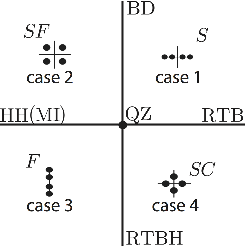
Figure 3: Sketch of the possible organization of spatial eigenvalues $\lambda$ satisfying the biquadratic equation (11) for a spatially reversible system. The names corresponding to the different labels are explained in Table 1.

Cod	$(\lambda_{1,2,3,4})$	Name	Label
Zero	$(\pm q_{0}\pm ik_{0})$	Saddle-Focus	$SF$
Zero	$(\pm q_{1},\pm q_{2})$	Saddle	$S$
Zero	$(\pm ik_{1},\pm ik_{2})$	Center	$F$
Zero	$(\pm q_{0},\pm ik_{0})$	Saddle-Center	$SC$
One	$(\pm q_{0},0,0)$	Rev.Takens-Bogdanov	RTB
One	$(\pm ik_{0},0,0)$	Rev.Takens-Bogdanov-Hopf	RTBH
One	$(\pm q_{0},\pm q_{0})$	Belyakov-Devaney	BD
One	$(\pm ik_{0},\pm ik_{0})$	Hamiltonian-Hopf	HH(MI)
Two	$(0,0,0,0)$	Quadruple Zero	QZ

Table 1: Nomenclature used to refer to different transitions in the spatial eigenspectrum.

The fixed points of Eq. (9) are the HSSs $A_{0}$ of the original evolution equation (2). The stability of these fixed points (in space) is determined by the eigenspectrum of the Jacobian of the system (9) around $A_{0}\equiv U_{0}+iV_{0}$, namely

$$\mathcal{J}=\nu\left[\begin{array}[]{cccc}0&0&\nu&0\\ 0&0&0&\nu\\ \theta-V^{2}-3U^{2}&1-2UV&0&0\\ -(1+2UV)&\theta-U^{2}-3V^{2}&0&0\\ \end{array}\right]_{(U_{0},V_{0})}.$$ (10)

The four eigenvalues of $\mathcal{J}$ satisfy the biquadratic equation

$$\lambda^{4}+(4I_{0}-2\theta)\nu\lambda^{2}+\theta^{2}+3I_{0}^{2}-4\theta I_{0}+1=0.$$ (11)

The form of this equation is a consequence of spatial reversibility Devaney ; Homburg ; Knobloch15 , i.e., the invariance of Eq. (2) under the transformation $(x,A)\mapsto(-x,A)$, or equivalently the invariance of the system (9) under $(x,U,V,\tilde{U},\tilde{V})\mapsto(-x,U,V,-\tilde{U},-\tilde{V})$. This invariance implies that if $\lambda$ is a spatial eigenvalue, so are $-\lambda$ and $\pm\lambda^{*}$, where ^∗ indicates complex conjugation. Consequently there are four possibilities:

1. the eigenvalues are real: $\lambda_{1,2,3,4}=(\pm q_{1},\pm q_{2})$

2. there is a quartet of complex eigenvalues: $\lambda_{1,2,3,4}=(\pm q_{0}\pm ik_{0})$

3. the eigenvalues are imaginary: $\lambda_{1,2,3,4}=(\pm ik_{1},\pm ik_{2})$

4. two eigenvalues are real and two imaginary: $\lambda_{1,2,3,4}=(\pm q_{0},\pm ik_{0})$.

A sketch of these possible eigenvalue configurations is shown in Fig. 3, and their names and codimension are provided in Table 1. The transition from case 1 to case 2 is through a Belyakov-Devaney (BD) Champneys ; Haragus point with eigenvalues $(\pm q_{0},\pm q_{0})$, while the transition from case 2 to case 3 is via a Hamiltonian-Hopf (HH) bifurcation Ioos ; Haragus , with $\lambda_{1,2,3,4}=(\pm ik_{0},\pm ik_{0})$. The transition from case 1 to case 4 is via a reversible Takens-Bogdanov (RTB) bifurcation with eigenvalues $\lambda_{1,2,3,4}=(\pm q_{0},0,0)$ Champneys ; Haragus while the transition from case 3 to case 4 is via a reversible Takens-Bogdanov-Hopf (RTBH) bifurcation with eigenvalues $\lambda_{1,2,3,4}=(\pm ik_{0},0,0)$ Champneys ; Haragus . The unfolding of all these scenarios is related to the quadruple zero (QZ) codimension-2 point Champneys ; Haragus . As shown in the next section the transitions between these different regimes organize the parameter space for DSs.

The eigenvalues satisfying Eq. (11) are

$$\lambda=\pm\sqrt{(\theta-2I_{0})\nu\pm\sqrt{I_{0}^{2}-1}}.$$ (12)

Figure 2 summarizes the possible eigenvalue configurations for normal dispersion ($\nu=-1$). The transition at $I_{0}=1$, i.e., along the green curve

$$\rho=\sqrt{1+(1-\theta)^{2}}$$ (13)

in Fig. 4, corresponds to a BD transition when $\theta<2$ and an HH transition when $\theta>2$. Figures 2(a)-(b) correspond to the case $\theta<2$; we see that the saddle-node bifurcation at SN_hom,1 corresponds to a RTB bifurcation. In contrast, for $\theta>2$ SN_hom,1 has become a RTBH bifurcation (Fig. 2(d)). For $\theta=2$ (Fig. 2(c)) the BD, HH, RTB and RTBH lines meet at the QZ point. In the parameter space of Fig. 4 the QZ point corresponds to $(\theta,\rho)=(2,\sqrt{2})$. The other relevant bifurcation lines in this scenario correspond to SN_hom,2. This point corresponds to a RTB bifurcation in space regardless of the value of $\theta$.

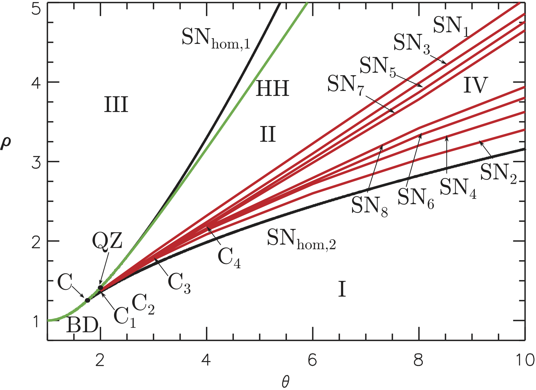
Figure 4: (Color online) The $(\theta,\rho)$ parameter space for normal dispersion in the region of existence of dark solitons. The green line corresponds to the HH bifurcation, the black lines to SN bifurcations of the HSS, and the red lines to SN bifurcations of the dark DSs. The bifurcation lines and the regions I–IV are discussed in more detail in the text.

In terms of spatial dynamics, DSs correspond to intersections of the stable and unstable manifolds of the HSS Knobloch15 . In cases 1 and 2 the HSS has a 2-dimensional stable and a 2-dimensional unstable manifold. These manifolds are transverse to the 2-dimensional fixed point subspace of the symmetry $(x,A)\mapsto(-x,A)$ and hence intersect in a structurally stable way. Therefore we expect DSs in cases 1 and 2 only. In case 4, the stable and unstable manifolds of the HSS are 1-dimensional and DSs, although possible, are exceptional Kolossovski . In Fig. 2(b) DSs bifurcate from both SN_hom,1 and SN_hom,2. When HH is present (Fig. 2(d)) DSs bifurcate from HH and from SN_hom,2.

In Sec. IV we show that it is possible to compute DSs analytically near the bifurcation points that produce them, and use the resulting expressions to initialize numerical continuation algower of these states.

IV Bifurcations and existence of dissipative solitons

IV.1 Weakly nonlinear analysis

In this section we compute weakly nonlinear DSs using multiple scale perturbation theory near the RTB bifurcation corresponding to SN_hom,2. The procedure applies equally around the other RTB point at SN_hom,1. Following BuYoKn , we fix the value of $\theta$ and suppose that the DSs at $\rho\approx\rho_{t}$, where $\rho=\rho_{t}$ corresponds to the SN_hom,2 bifurcation, are captured by the ansatz $U=U^{*}+u$, $V=V^{*}+v$, where $U^{*}$ and $V^{*}$ represent the HSS $A_{0}^{t}$ and $u$ and $v$ capture the spatial dependence. We next introduce appropriate asymptotic expansions for each variable in terms of a small parameter $\epsilon$ defined through the relation $\rho=\rho_{t}+\epsilon^{2}\delta$, where $\delta$ is defined in the Appendix. Each variable is written in the form

$$\left[\begin{array}[]{c}U^{*}\\ V^{*}\end{array}\right]=\left[\begin{array}[]{c}U_{t}\\ V_{t}\end{array}\right]+\epsilon\left[\begin{array}[]{c}U_{1}\\ V_{1}\end{array}\right]+...$$ (14)

and

$$\left[\begin{array}[]{c}u\\ v\end{array}\right]=\epsilon\left[\begin{array}[]{c}u_{1}\\ v_{1}\end{array}\right]+\epsilon^{2}\left[\begin{array}[]{c}u_{2}\\ v_{2}\end{array}\right]+...$$ (15)

and these expressions inserted into Eq. (3). Solving order by order in $\epsilon$ we find that the leading order asymptotic solution close to the RTB point is given by

$$\left[\begin{array}[]{c}U\\ V\end{array}\right]=\left[\begin{array}[]{c}U_{t}\\ V_{t}\end{array}\right]+\epsilon\left[\begin{array}[]{c}U_{1}+u_{1}\\ V_{1}+v_{1}\end{array}\right],$$ (16)

where $U_{t}$ and $V_{t}$ correspond to the HSS at $\rho=\rho_{t}$, and

$$\left[\begin{array}[]{c}u_{1}\\ v_{1}\end{array}\right]=\left[\begin{array}[]{c}U_{1}\\ V_{1}\end{array}\right]\psi(x),$$ (17)

with

$$\left[\begin{array}[]{c}U_{1}\\ V_{1}\end{array}\right]=\mu\left[\begin{array}[]{c}1\\ \eta\end{array}\right]$$ (18)

and

$$\psi(x)=-3{\textnormal{sech}}^{2}\left[\displaystyle\frac{1}{2}\sqrt{-\frac{\alpha_{2}}{\alpha_{1}}}\left(\displaystyle\frac{\rho-\rho_{t}}{\delta}\right)^{1/4}x\right].$$ (19)

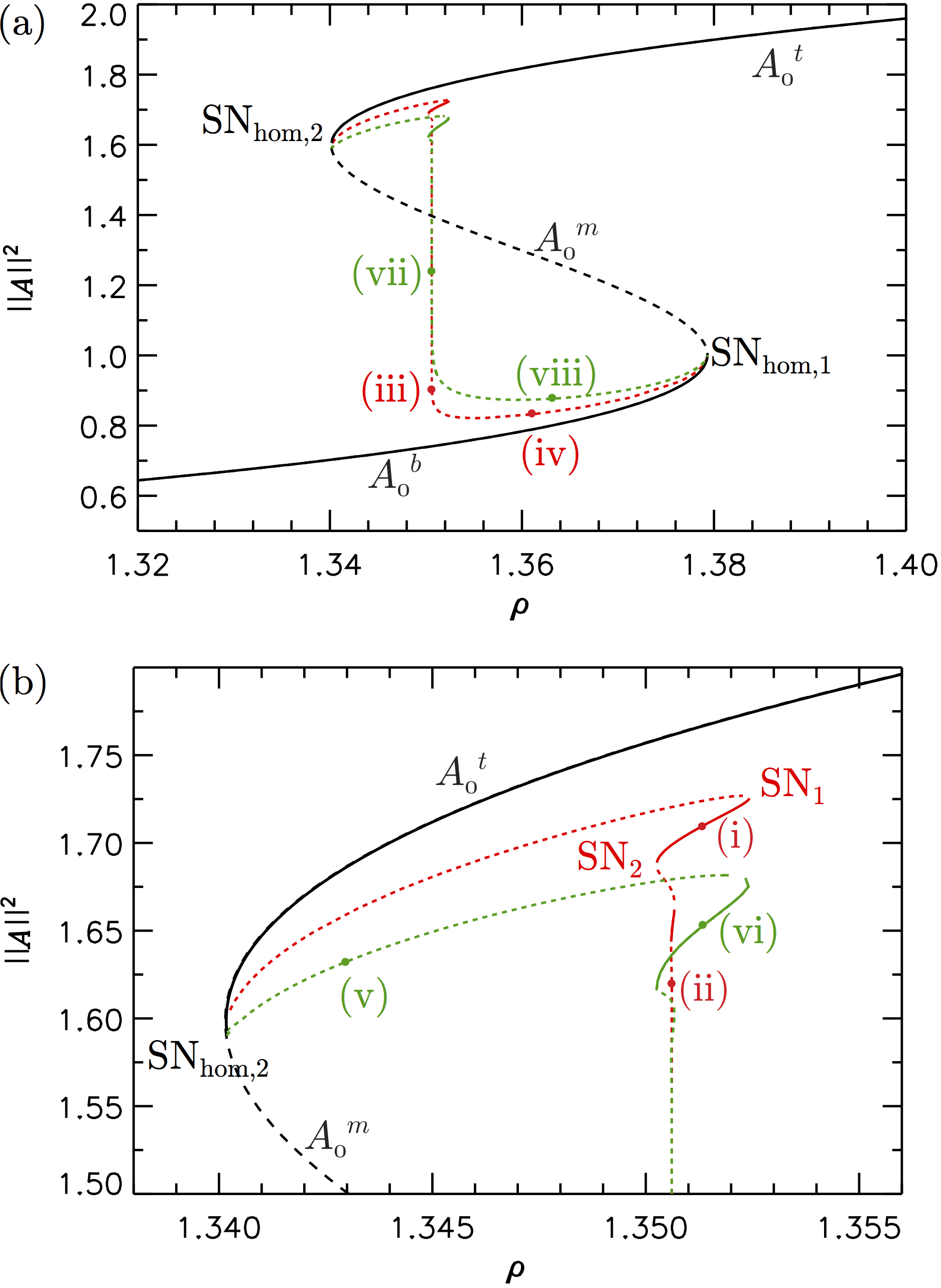
Figure 5: (a) Bifurcation diagram at $\theta=1.95$. (b) Zoom of panel (a) around SN_hom,2. The homogeneous steady states HSS are shown in black, 1-soliton states in red and 2-soliton states in green. Temporally stable (unstable) DSs are indicated using solid (dashed) lines. Profiles corresponding to the labeled locations are shown in Fig. 6 and in more detail in Fig. 7.

Here $\eta$, $\mu$, $\alpha_{1}$ and $\alpha_{2}$ are parameters defined in the Appendix, where the details of the calculation can be found. The localized structure defined by the asymptotic solution is shown in Fig. 22 of the Appendix; the negative sign in Eq. (19) implies that the solution is a hole in the background $A_{0}^{t}$ state, i.e., a dark soliton. Of course, on a large domain we expect to find states with 2 or more dark solitons as well. When these are well separated these states behave like 1-soliton states and so should bifurcate from the vicinity of SN_hom,2 just like the 1-soliton states.

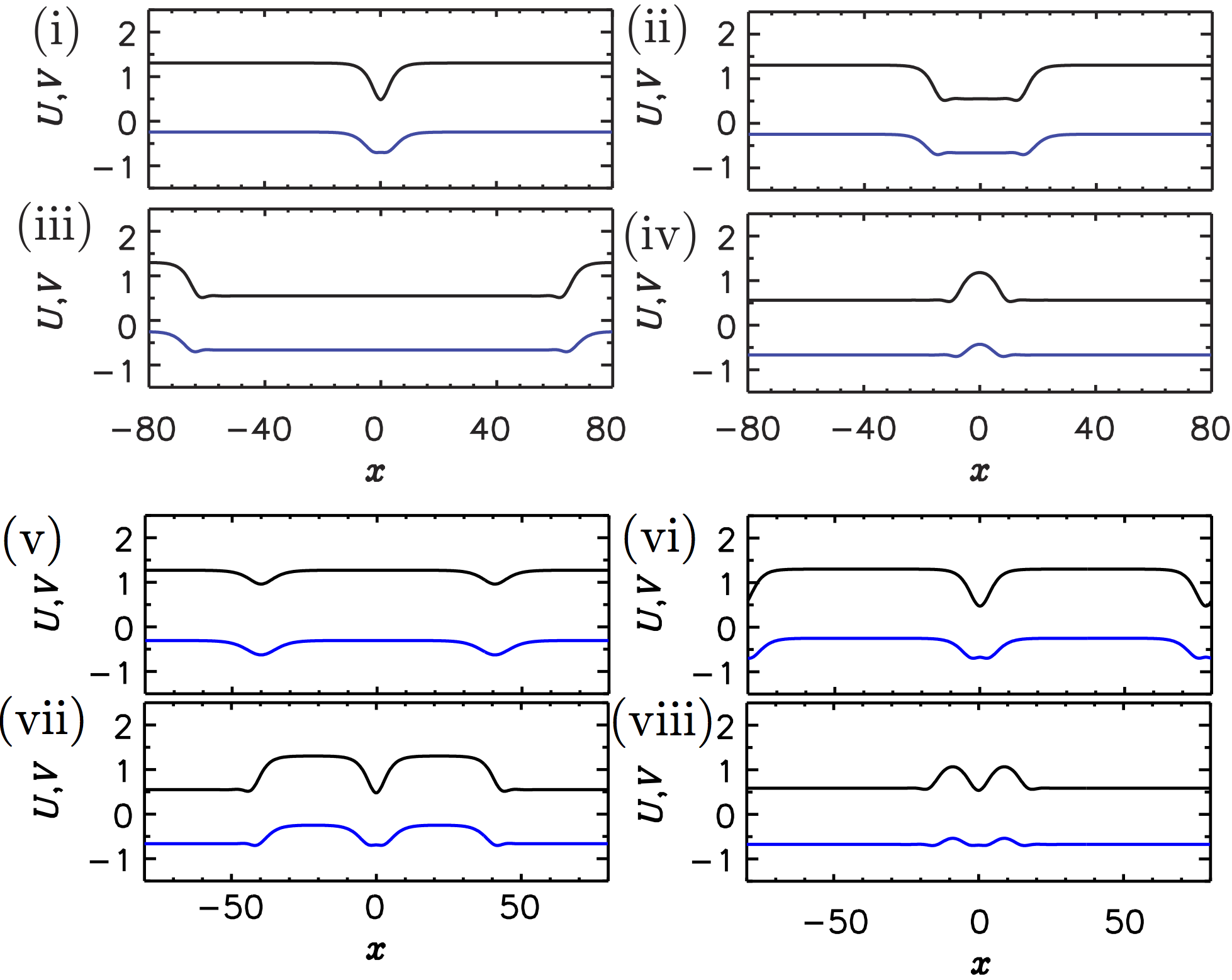
Figure 6: (Color online) Spatial profiles of DSs (dark and bright 1-soliton and 2-soliton states) corresponding to the locations indicated in Fig. 5(a,b), with $U(x)$ in black and $V(x)$ in blue. Near SN_hom,2 the states resemble holes (dark solitons) while near SN_hom,1 they resemble localized pulses (bright solitons).

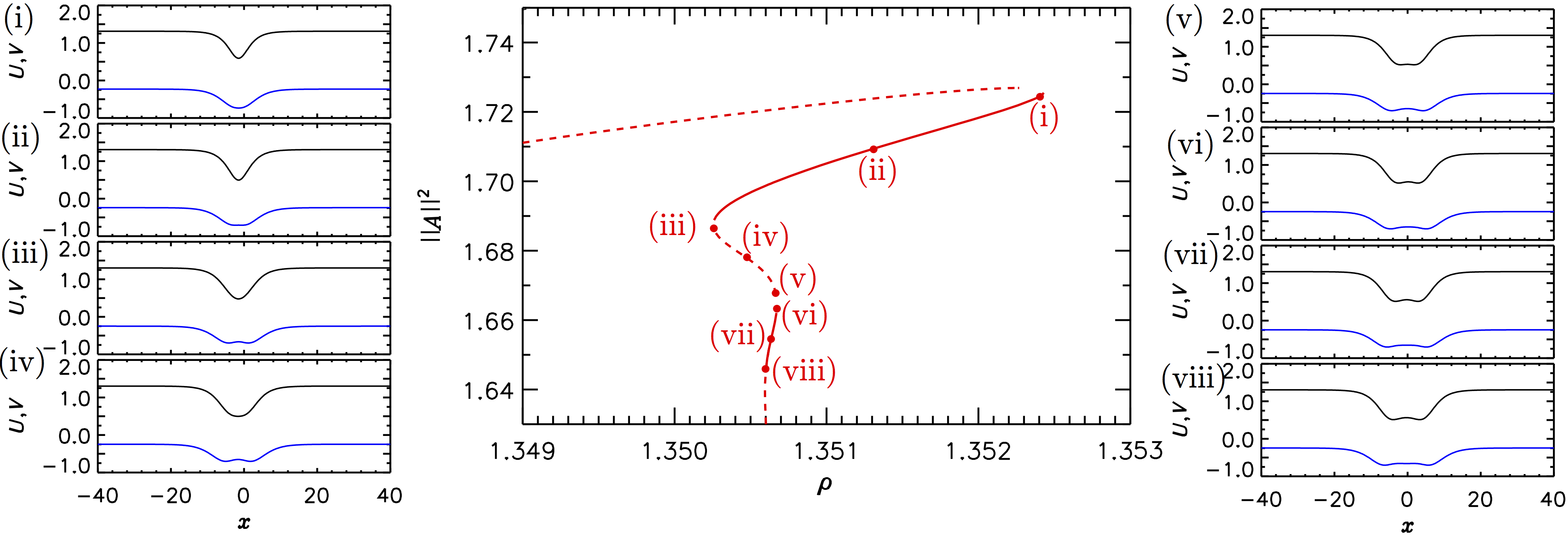
Figure 7: (Color online) Spatial profiles of dark solitons near the upper end of the $\theta=1.95$ 1-soliton branch at locations indicated in the middle panel, showing that the splitting of the central peak (dip) in $(U(x),V(x))$, shown in black and red, respectively, occurs at different locations along the branch.

We now discuss the bifurcation structure of dark solitons in two regimes: the bistable region before the QZ point, namely for $\sqrt{3}<\theta<2$, and the bistable region after QZ, i.e., for $\theta>2$.

IV.2 Dark solitons for $\sqrt{3}<\theta<2$

In the following we use the $L^{2}$ norm, $||A||^{2}\equiv\frac{1}{L}\int_{0}^{L}|A|^{2}\,dx$, to represent the DSs in a bifurcation diagram. Figure 5(a), computed for $\theta=1.95$, reveals the presence of two soliton branches, the first of which consists of a single dark soliton in the domain (hereafter the 1-soliton state, red branch) while the second consists of a pair of identical equidistant dark solitons in the domain (hereafter the 2-soliton state, green branch). Figure 5(b) provides a zoom of the region near SN_hom,2. Both branches bifurcate from HSS very close to SN_hom,2 as anticipated in the preceding section and both undergo collapsed snaking KnWa ; BuYoKn_colapsing . Specifically, the 1-soliton state bifurcates from HSS closer to the saddle node at $\rho=\rho_{t}$ and its solution branch undergoes a series of exponentially decaying oscillations in the vicinity of a critical value of $\rho$, hereafter $\rho=\rho_{M}\approx 1.3506074$. During this process the hole corresponding to the dark soliton deepens, forming a pair of fronts connecting $A_{0}^{t}$ and $A_{0}^{b}$ and then broadens as the $A_{0}^{b}$ state expels $A_{0}^{t}$ (Fig. 6), becoming in an infinite system a heteroclinic cycle between $A_{0}^{t}$ and $A_{0}^{b}$ at $\rho_{M}$. In gradient systems this point corresponds to the so-called Maxwell point, where both homogeneous solutions have equal energy. In non-gradient systems, such as LLE, such a cycle may still be present, even though an energy cannot be defined, and we retain this terminology to refer to its location, i.e., the parameter value corresponding to the presence a pair of stationary, infinitely separated fronts connecting $A_{0}^{t}$ to $A_{0}^{b}$ and back again.

The successive saddle nodes seen in Fig. 5 correspond to the appearance of additional oscillations in the tails of the fronts as the local maximum (minimum) at the symmetry point $x=0$ turns into a local minimum (maximum) and back again, and hence to a gradual increase in the width of the hole. Figure 7 shows a detail of this process. The associated hole states are temporally stable between SN₁ and SN₂, and on all the subsequent branch segments with positive slope KnWa ; BuYoKn_colapsing , shown using solid lines. A profile of a stable localized hole on the SN₁–SN₂ segment is shown in Fig. 6(i). For the value of $\theta$ used in Fig. 5 the collapse of the saddle nodes to $\rho_{M}$ is very abrupt because the spatial oscillations in the tail of the front decay very fast. Figure 8 shows a clearer example of the behavior in this region, albeit for a larger value of $\theta$.

In finite systems the hole or 1-soliton branch departs from $\rho\approx\rho_{M}$ when the maximum amplitude starts to decrease below $A_{0}^{t}$ and the solution turns into a bright soliton sitting on top of $A_{0}^{b}$ (Fig. 6(iv)). The branch then terminates at SN_hom,1, where the amplitude of this soliton falls to zero. On an infinite domain the DS branches bifurcating from SN_hom,2 and SN_hom,1 remain distinct and do not connect up. Figures 5 and 6 show that the 2-soliton branch behaves in a very similar manner. In fact, this is so for all $n$-soliton branches ($n\geq 3$), provided the solitons remain sufficiently well separated.

IV.3 Dark solitons for $\theta>2$

For $\theta>2$ the saddle node SN_hom,1 becomes a RTBH point with spatial eigenvalues $\lambda_{1,2,3,4}=(0,0,\pm ik_{0})$ and homoclinic orbits are exceptional BuYoKn ; Kolossovski . However, in this case this point is preceded by a HH bifurcation on $A_{0}^{b}$, which gives rise to a branch of PSs. The PSs bifurcate subcritically (Fig. 8) but remain unstable throughout their existence range, despite the presence of a saddle node. This is the case for all values of the detuning $\theta$ we explored ($2.3<\theta<10$). Thus no bistability between PS and $A_{0}^{b}$ results and no snaking of bright DSs takes place Champneys ; gomila_Scroggi . Instead the bright solitons bifurcating from HH connect to the dark solitons originating at $\rho=\rho_{t}$, as we now discuss.

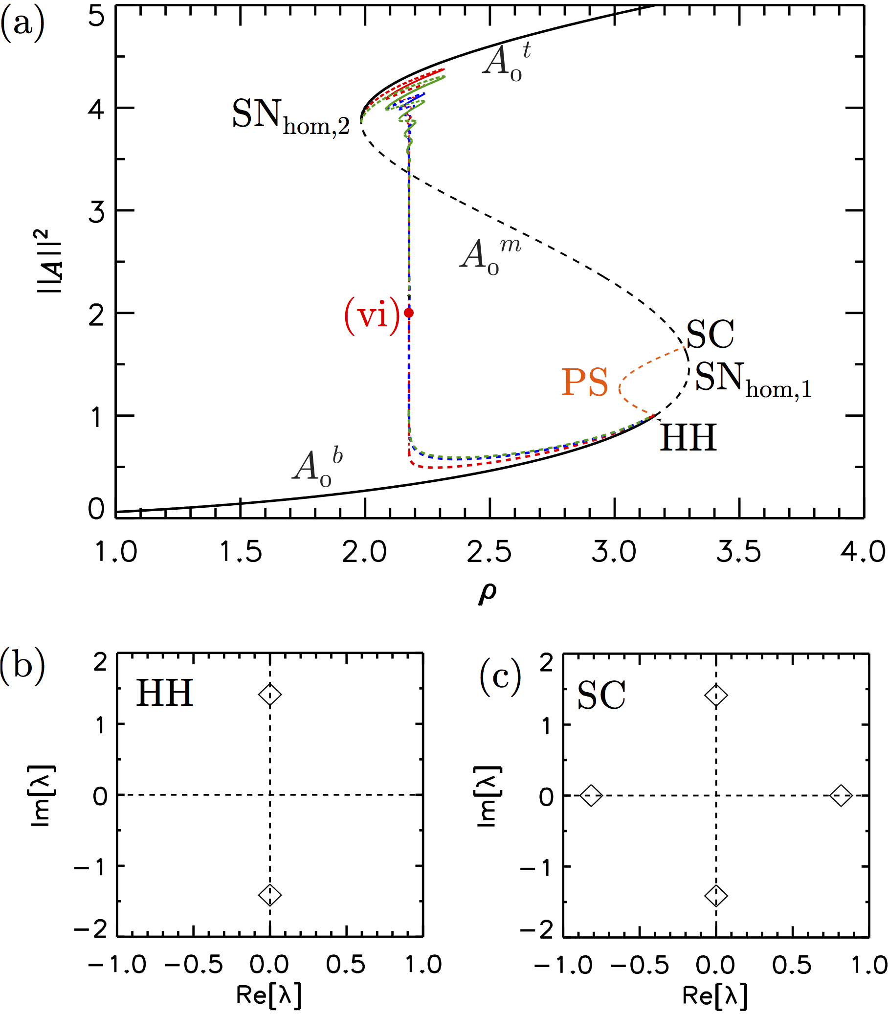
Figure 8: (Color online) (a) Bifurcation diagram for $\theta=4$ showing collapsed defect-mediated snaking of 1-soliton (red line) and 2-soliton (green line) branches, showing their reconnection with the PS branch (orange line) that bifurcates from HH on $A_{0}^{b}$. Temporally stable (unstable) structures are indicated using solid (dashed) lines. Black lines correspond to HSS. Enlargements of panel (a) can be found in Figs. 10 and 12. (b) The spatial eigenvalues $\lambda$ of $A_{0}$ at locations HH and SC in (a).

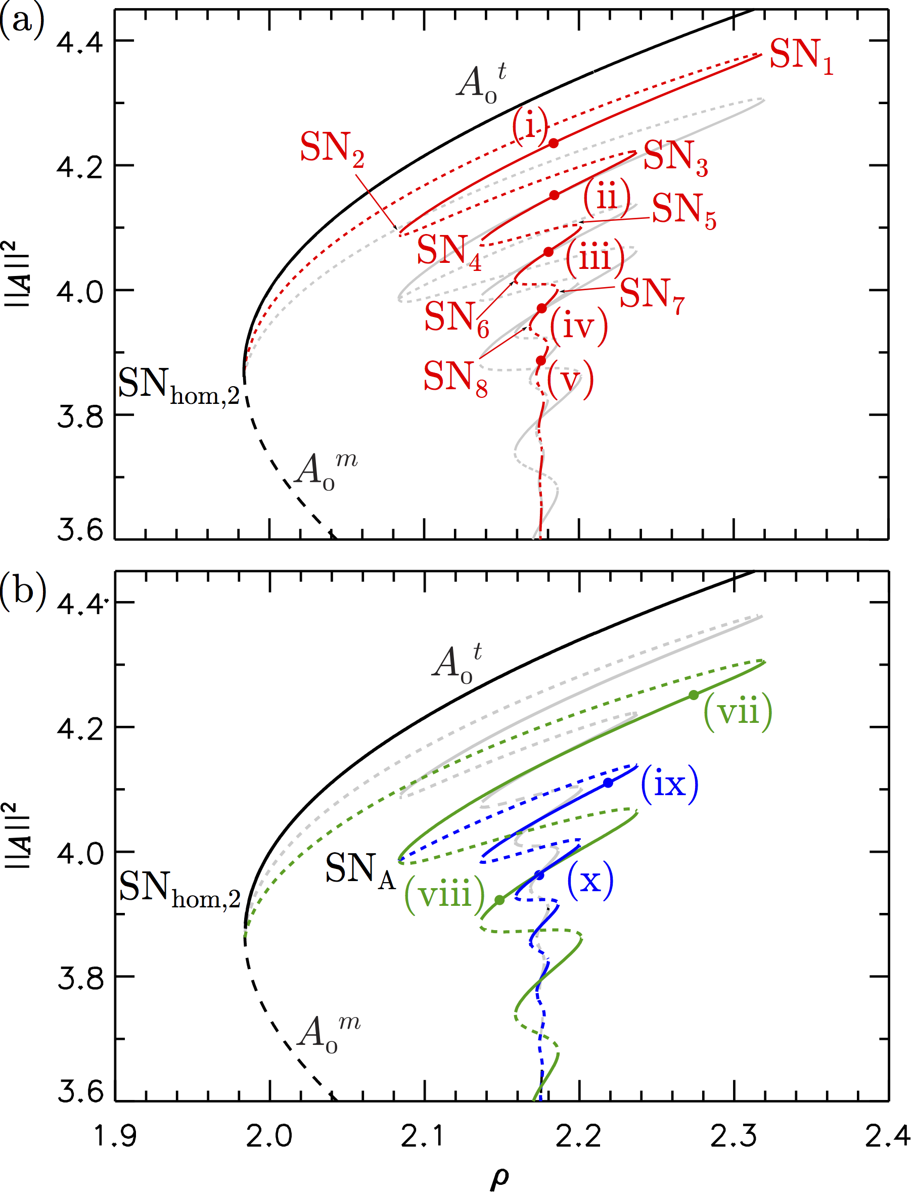
Figure 9: (Color online) Detail of the 1-soliton (panel (a), red line) and 2-soliton (panel (b), green line) branches in the vicinity of SN_hom,2 for $\theta=4$. Black lines show the homogeneous states HSS. Panel (b) also shows a family of nonidentical 2-soliton states (blue line) that bifurcate from the saddle node SN_A on the 2-soliton branch and also undergo collapsed defect-mediated snaking. Temporally stable (unstable) structures are indicated using solid (dashed) lines. Profiles corresponding to the labeled locations are shown in Fig. 10, with details of this process shown in Fig. 11.

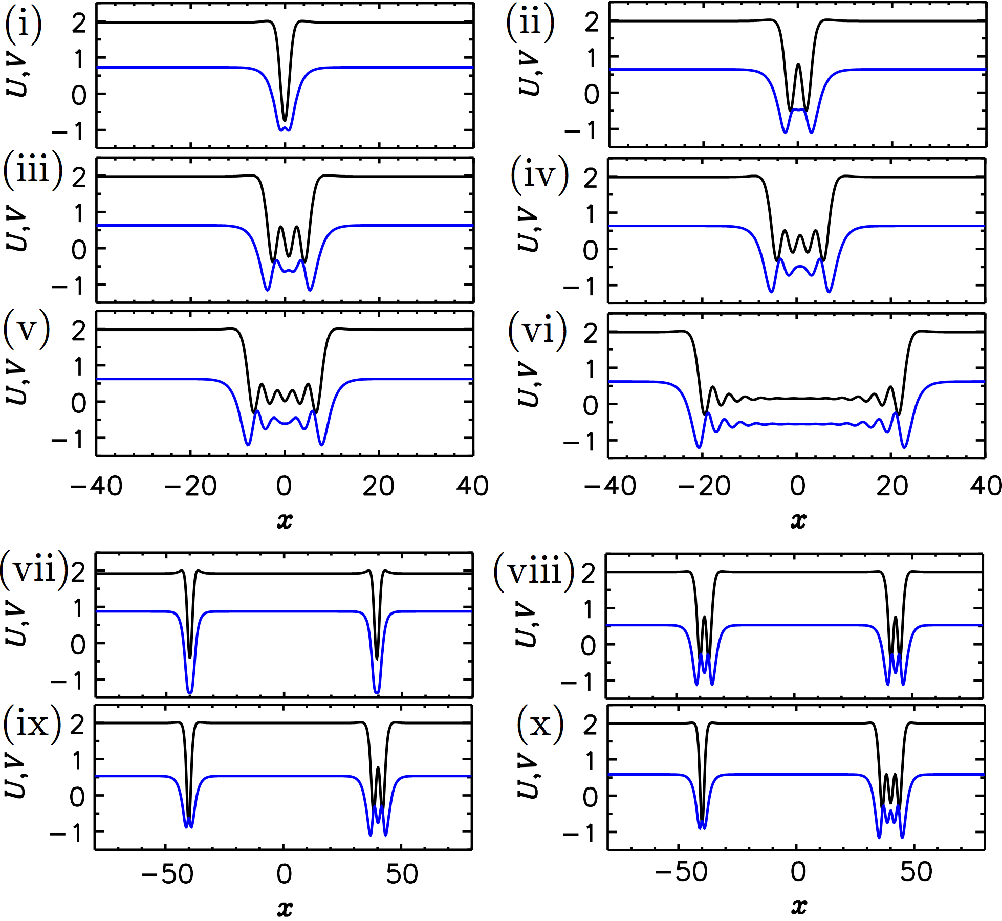
Figure 10: (Color online) Spatial profiles of the solutions represented in Fig. 8(a) for $\theta=4$, showing $U(x)$ in black and $V(x)$ in blue. Panels (i)-(vi) correspond to 1-soliton states (red branches in Figs. 8(a) and 10(a)), panels (vii)-(viii) to 2-soliton states (green branches in Figs. 8(a) and 10(b)) and panels (ix)-(x) to the branch of nonidentical 2-soliton states (blue branch in Fig. 10(b)).

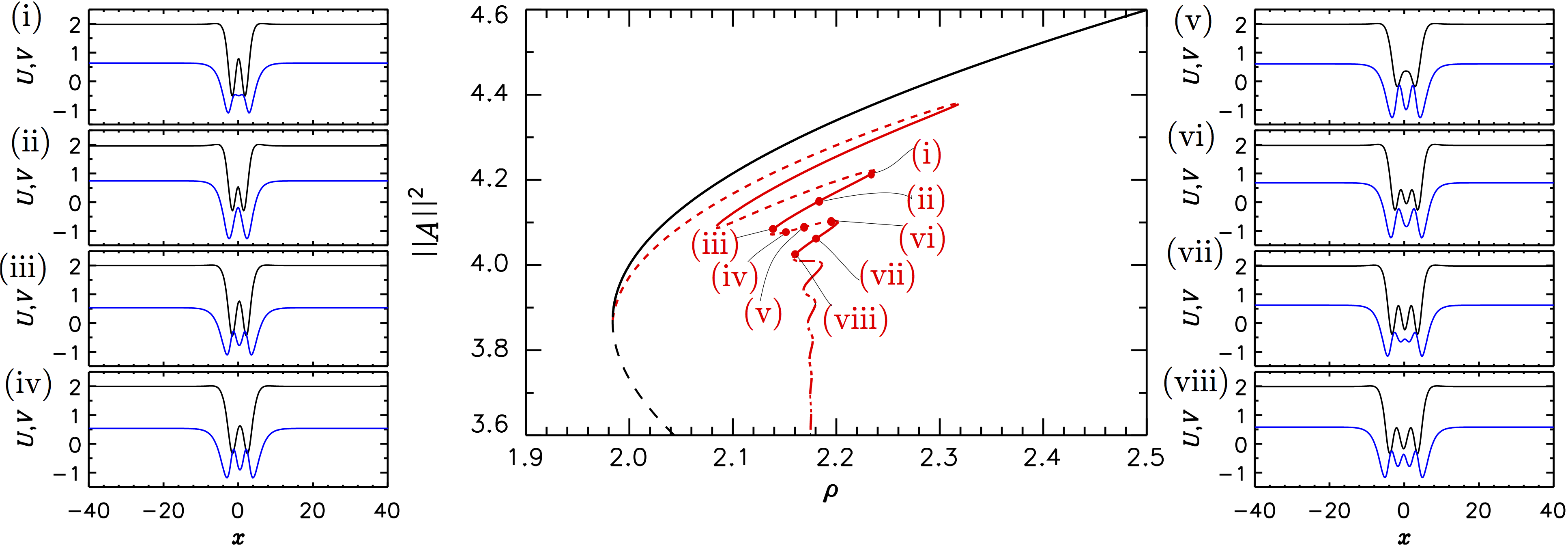
Figure 11: (Color online) Spatial profiles of the dark solitons near the upper end of the $\theta=4$ 1-soliton branch at locations indicated in the middle panel, showing that the splitting of the central peak (dip) in $(U(x),V(x))$, shown in black and red, respectively, occurs at different locations along the branch.

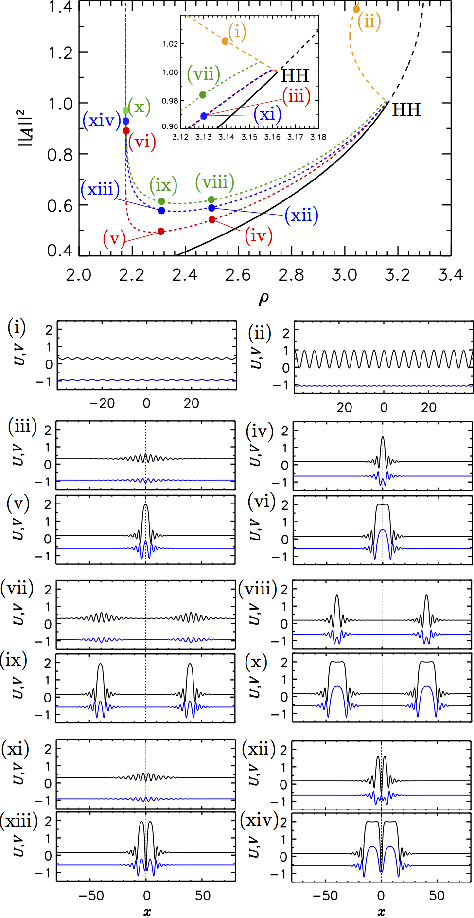
Figure 12: (Color online) Bifurcation diagram for $\theta=4$ (top panel) showing the bifurcation of the three families of localized states (bright solitons) from the subcritical PS branch, together with sample solution profiles corresponding to the locations indicated in the top panel. States with maxima at $x=0$ (red line) connect with the corresponding branch of dark solitons shown in Figs. 8(a) and 10(a) while states with minima at $x=0$ (blue line) connect with the corresponding branch in Fig. 10(b). The states shown in green consist of two equidistant bright solitons and these connect to the corresponding branch in Fig. 10(b).

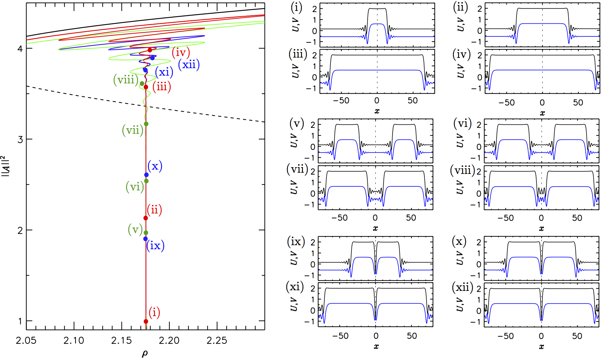
Figure 13: Details of the profile transformation at $\theta=4$ that changes two nonidentical dark solitons (blue branch in Fig. 10(b)) into a bright soliton with a minimum at its center $x=0$, allowing it to connect to the PS state at the same location as the 1-soliton state (red branch in Fig. 10(a)) which evolves into a bright soliton with a maximum at its center $x=0$. The 2-soliton state consisting of two identical equidistant solitons (green branch in Fig. 10(b)) also terminates on PS, but at a distinct location.

Figure 8(a) shows the bifurcation diagram of the 1-soliton states (red branch) for $\theta=4$ obtained by numerically continuing the analytical prediction obtained in Eq. (19) away from SN_hom,2. Figure 10(a) shows a detail of this branch. These states are initially unstable but as $\rho$ increases these unstable 1-soliton states grow in amplitude and acquire stability at saddle node SN₁. The DS profile on this segment of the branch is shown in Fig. 10(i). This solution loses stability at SN₂ but starts to develop a spatial oscillation (SO) in the center; solutions of this type become stable at SN₃. An example of the resulting stable solution can be found in Fig. 10(ii). This process repeats in such a way that between successive saddle nodes on the left or right a new spatial oscillation is inserted in the center of the dark soliton profile and the soliton broadens, decreasing its $L^{2}$ norm. As a result, as one proceeds down the snaking branch the central peak (dip) repeatedly splits. Details of this process are shown in Fig. 11. The resulting behavior resembles in all aspects the phenomenon of defect-mediated snaking described in BuYoKn_colapsing except for the exponential shrinking of the region of existence of these states as the hole broadens. Consequently we refer to this behavior as collapsed defect-mediated snaking. Numerically the collapse occurs at $\rho=\rho_{M}\approx 2.1753479$. The DSs at this location correspond to broad hole-like states of the type shown in Fig. 10(v). As in Sec. IV.2 further decrease in the norm signals that the two fronts connecting states $A_{0}^{t}$ and $A_{0}^{b}$ at $\rho_{M}$ are starting to separate (Fig. 10(vi)); this process continues, resulting in the bright soliton state shown in Fig. 12(iv); this state is shifted by half the domain width relative to panels (i)-(vi) of Fig. 10. Thereafter the amplitude of the peak at $x=0$ starts to decrease and the 1-soliton branch departs from $\rho_{M}$, ultimately connecting to the branch of small amplitude PS (Fig. 12(i)) that bifurcates subcritically from HH (see inset in Fig. 12, top panel).

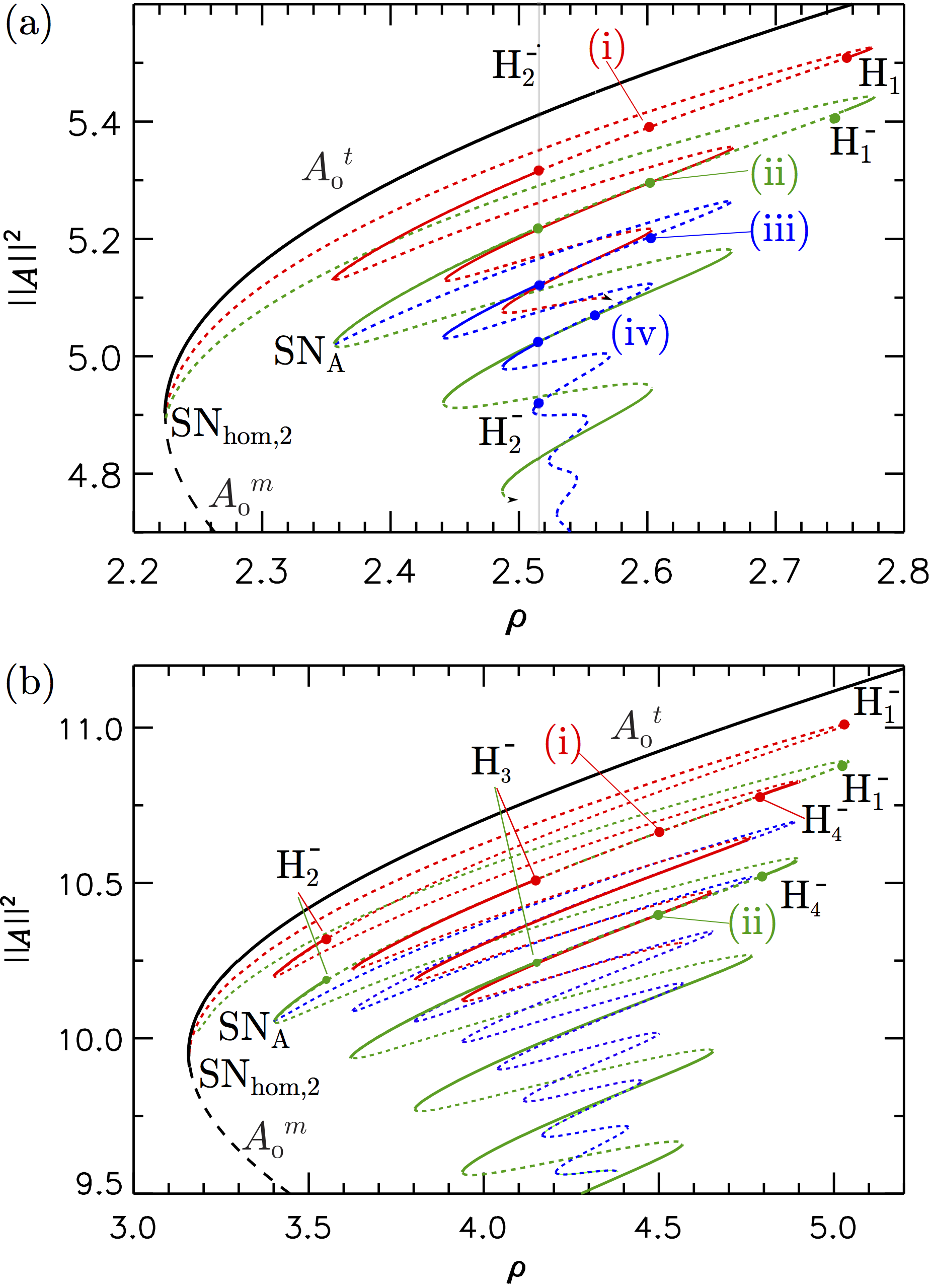
Figure 14: (Color online) Bifurcation diagram for (a) $\theta=5$ and (b) $\theta=10$ showing that the DSs are now unstable within intervals between back-to-back Hopf bifurcations. The Hopf bifurcations on the left (H${}^{-}_{2}$, panel (a)) for the 2-soliton states (green and blue lines) coincide with that of the 1-soliton states (red line).

Figure 8(a) also shows the 2-soliton state (green line) that bifurcates from the vicinity of SN_hom,2 for $\theta=4$ just as in the case $\theta=1.95$. For $\theta>2$ this second DS family plays a key role since it is responsible for providing the second of the two branches of localized states that are known to be associated with HH. Figures 10(b), 12 and 13 show how this happens. The green branch in Fig. 10(b) consists of states with identical equidistant solitons; like the 1-soliton states, the 2-soliton states proceed to develop internal oscillations (Figs. 10(vii)-(viii)). These undergo a symmetry-breaking pitchfork bifurcation at SN_A giving rise to a branch of nonidentical solitons (in blue). One of these gradually acquires complex internal structure while the other remains unchanged. Figures 10(ix)-(x) show this state at the locations shown in Fig. 10(b), while Fig. 13(xii) shows a translate of such a 2-soliton state by a quarter of the domain size. Figures 13(xii)-(ix) and 12(xiv)-(xi) show the subsequent evolution of this 2-soliton state into a single wave packet with a minimum at its center $x=0$. It is this state that connects to PS at the same location as the corresponding wave packet (red) with a maximum at $x=0$ that originates in the 1-soliton state near SN_hom,2. In contrast, the 2-soliton state that also appears near SN_hom,2 (green) terminates in a distinct bifurcation on PS, as also shown in Fig. 12. All three branches undergo collapsed defect-mediated snaking inbetween. Evidently there are similar branches that bifurcate from other folds on the 2-soliton branch (not shown).

We mention that as the domain length increases the termination point of the 1-soliton (red line) and the nonidentical 2-soliton branch (blue line) migrates towards HH and in the limit of an infinite domain the bright solitons bifurcate from $A_{0}^{b}$ simultaneously with the PS, exactly as predicted by the normal form for the spatial Hopf bifurcation with 1:1 resonance Ioos . We also mention that, in principle, the Maxwell point $\rho_{M}$ may collide with the saddle node of the PS branch (see Ma for details). However, we have determined that such a collision does not occur in the LLE and that the PS branch remains well-separated from the collapsed snaking branches of dark solitons around $\rho_{M}$ (at least in the parameter range $2.3<\theta<10$).

We turn, finally, to the structure of the spatial eigenvalues shown in Fig. 8(b,c). Panel (b) confirms that HH corresponds to a Hamiltonian-Hopf bifurcation in space. Panel (c) shows that at the termination point of the PS branch the HSS state $A_{0}^{m}$ has 2 purely real and 2 purely imaginary spatial eigenvalues, indicating that SC corresponds to a global bifurcation in space and not a local bifurcation. Both HH and SC are formed in the process of unfolding the spatially reversible QZ bifurcation that takes place at SN_hom,1 when $\theta=2$.

IV.4 Soliton location in the $(\theta,\rho)$ plane

Tracking each bifurcation point in the bifurcation diagram as a function of $\theta$ we obtain the $(\theta,\rho)$ parameter plane shown in Fig. 4. The green solid line represents a BD transition for $\theta<2$ that turns into a HH bifurcation for $\theta>2$. The saddle-node bifurcations determine the regions of existence of the different dark solitons shown previously. With increasing $\theta$ the region of existence of these states becomes broader (Fig. 14(a,b)). In contrast, when $\theta$ decreases the branches of solutions with several SO progressively shrink, disappearing in a series of cusp bifurcations C₁,…,C₄, as shown in Fig. 4.

We distinguish four main dynamical regions, labeled I to IV in the phase diagram in Fig. 4, on the basis of the existence of HSS and dark DSs:

• Region I: The bottom HSS $A_{0}^{b}$ is stable. No dark DSs or top HSS $A_{0}^{t}$ exist. This region spans the parameter space $\rho<\rho_{BD}$ for $\theta<\sqrt{3}$ and $\rho<\rho_{SN_{hom,2}}$ for $\theta>\sqrt{3}$.

• Region II: The bottom HSS $A_{0}^{b}$ and top HSS $A_{0}^{t}$ coexist and are both stable. No dark DSs are found. This region spans the parameter space $\rho_{SN_{1}}<\rho<\rho_{SN_{hom,1}}$ for $\theta>\sqrt{3}$.

• Region III: The top HSS $A_{0}^{t}$ is stable. No dark DSs or bottom HSS $A_{0}^{b}$ exist. This region spans the parameter space $\rho>\rho_{BD}$ for $\theta<\sqrt{3}$ and $\rho>\rho_{SN_{hom,1}}$ for $\theta>\sqrt{3}$.

• Region IV: The bottom HSS $A_{0}^{b}$ and top HSS $A_{0}^{t}$ are stable and coexist with (possibly unstable) dark DSs. This region spans the parameter space $\rho_{SN_{hom,2}}<\rho<\rho_{SN_{1}}$ for $\theta>\sqrt{3}$.

Region IV is the main region of interest in this work. It can be further subdivided to reflect the locations of different types of DSs. In the next Section, we refer to the region between SN₁ and SN₂, i.e., the region of existence of 1-SO dark solitons, as subregion IV₁. Similarly, subregion IV₂ corresponds to 2-SO dark solitons between SN₃ and SN₄ and so on. While both HSS are stable in region IV, the stability of dark DSs in the various subregions depends on the parameter values ($\theta$,$\rho$) as discussed next.

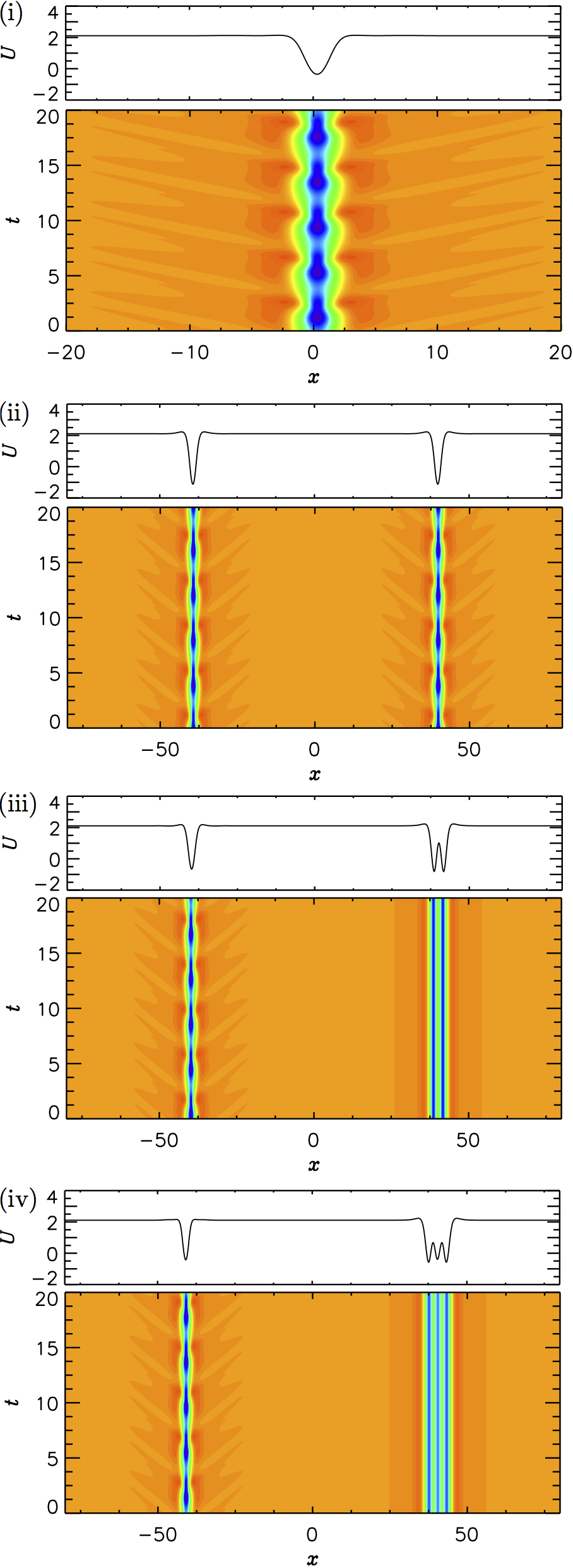
Figure 15: (Color online) (i) Oscillatory 1-soliton state, (ii) oscillatory 2-soliton state, (iii) a bound state of an oscillating and a stationary dark soliton, all computed for $\theta=5$, $\rho=2.6$. (iv) A similar state to panel (iii) but for $\theta=5$, $\rho=2.56$. The solutions are represented in a space-time plot of $U(x,t)$ with time increasing upwards. The profile at the final instant, $t=20$, is shown above each space-time plot.

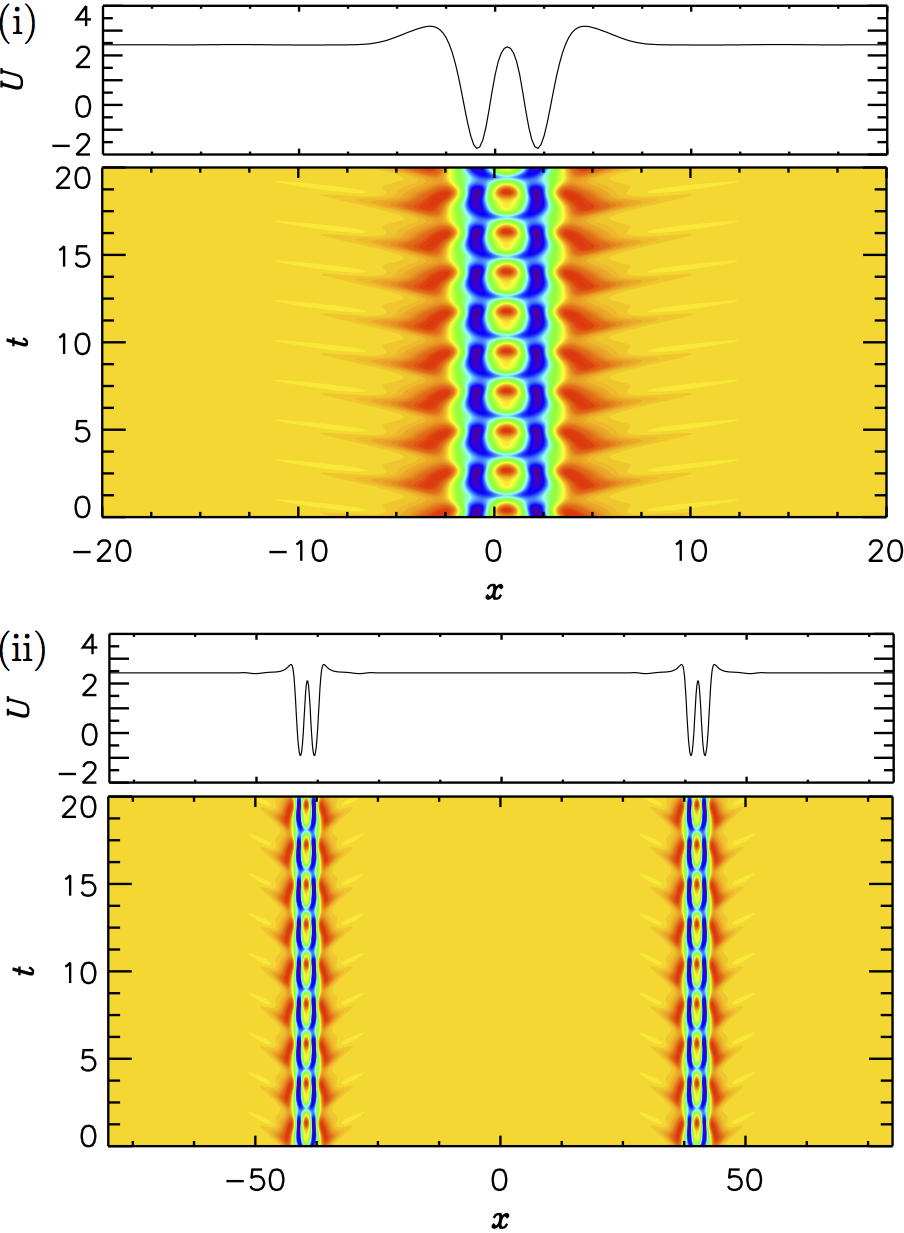
Figure 16: (Color online) (i) Oscillatory 1-soliton state, and (ii) oscillatory 2-soliton state, when $\theta=10$, $\rho=4.5$. The solutions are represented in a space-time plot of $U(x,t)$ with time increasing upwards. The profile at the final instant, $t=20$, is shown above each space-time plot.

V Oscillatory and chaotic dynamics

We have seen that the range of values of the parameter $\rho$ within which one finds dark solitons increases rapidly with increasing detuning $\theta$ although the interval with stable stationary dark solitons is reduced by the presence of oscillatory instabilities that set in as $\theta$ increases (Fig. 14). These intervals of instability open up on the stable portions of the collapsed snaking branches, between pairs of supercritical Hopf bifurcations on either side. Consequently these instabilities lead to stable temporal oscillations resembling breathing of the individual solitons. To characterize the resulting dynamics we combine here linear stability analysis in time with direct integration of the LLE. We also compute secondary bifurcations of time-periodic states and point out that in appropriate regimes the LLE exhibits dynamics that are very similar to those exhibited by excitable systems.

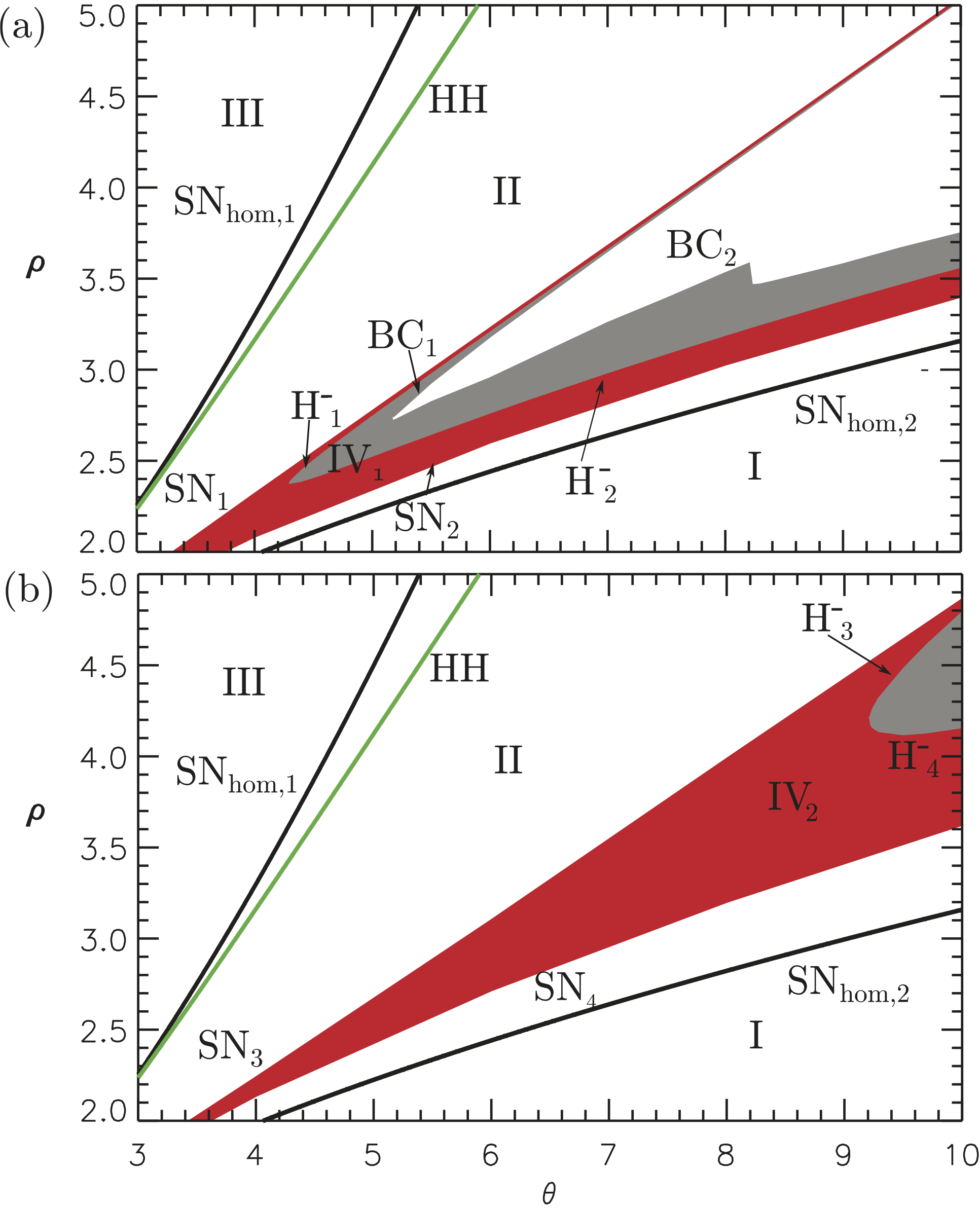
Figure 17: (Color online) The $(\theta,\rho)$ parameter space for normal dispersion ($\nu=-1$) showing the region of existence of (a) the 1-SO dark soliton and (b) the 2-SO dark soliton. The different bifurcations are labeled, with $H^{-}_{j}$ indicating a supercritical Hopf bifurcation at location $H_{j}$. The red (gray) region corresponds to stable stationary (oscillatory) dark DSs.

Figures 14(a) and (b) show that for both $\theta=5$ and $\theta=10$ the single dark soliton becomes unstable in a supercritical Hopf bifurcation (H${}^{-}_{1}$) leading to an oscillatory state. Figure 15(i) shows the resulting state at location (i) in Fig. 14(a). The temporal oscillations disappear upon further decrease in $\rho$ and do so in a reverse supercritical Hopf at H${}^{-}_{2}$, thereby restoring the stability of the single dark soliton. For larger values of $\theta$ this behavior not only persists but the soliton with 2 spatial oscillations (SO) also exhibits temporal oscillations between two back-to-back Hopf bifurcations (Fig. 14(b)). An example of such oscillatory 2-SO dark soliton is shown in Fig. 16(i).

Figure  15(ii) shows the corresponding oscillation of the 2-soliton state for $\theta=5$ at location (ii) in Fig. 14(a). The solitons oscillate in phase but in a nonsinusoidal manner. Figures 15(iii)-(iv) show oscillations of a bound state of two nonidentical dark solitons at locations (iii) and (iv) in Fig. 14(a). In these states the simple dark soliton on the left oscillates in a periodic fashion while the structured dark soliton on the right remains essentially time-independent. Figure 16(ii) shows a periodic oscillation of a 2-soliton state for $\theta=10$ corresponding to location (ii) in Fig. 14(b). The individual solitons are structured and oscillate as in panel (i). Once again, both oscillate in phase.

We can complete the parameter space shown in Fig. 4 by adding the curves corresponding to the oscillatory instabilities at H${}^{-}_{1}$ and H${}^{-}_{2}$. Figure 17 shows the parameter space with the curves corresponding to the temporal instabilities of the 1-SO and 2-SO dark solitons included; the saddle nodes of the remaining dark solitons are omitted in order to give a clearer understanding of this behavior.

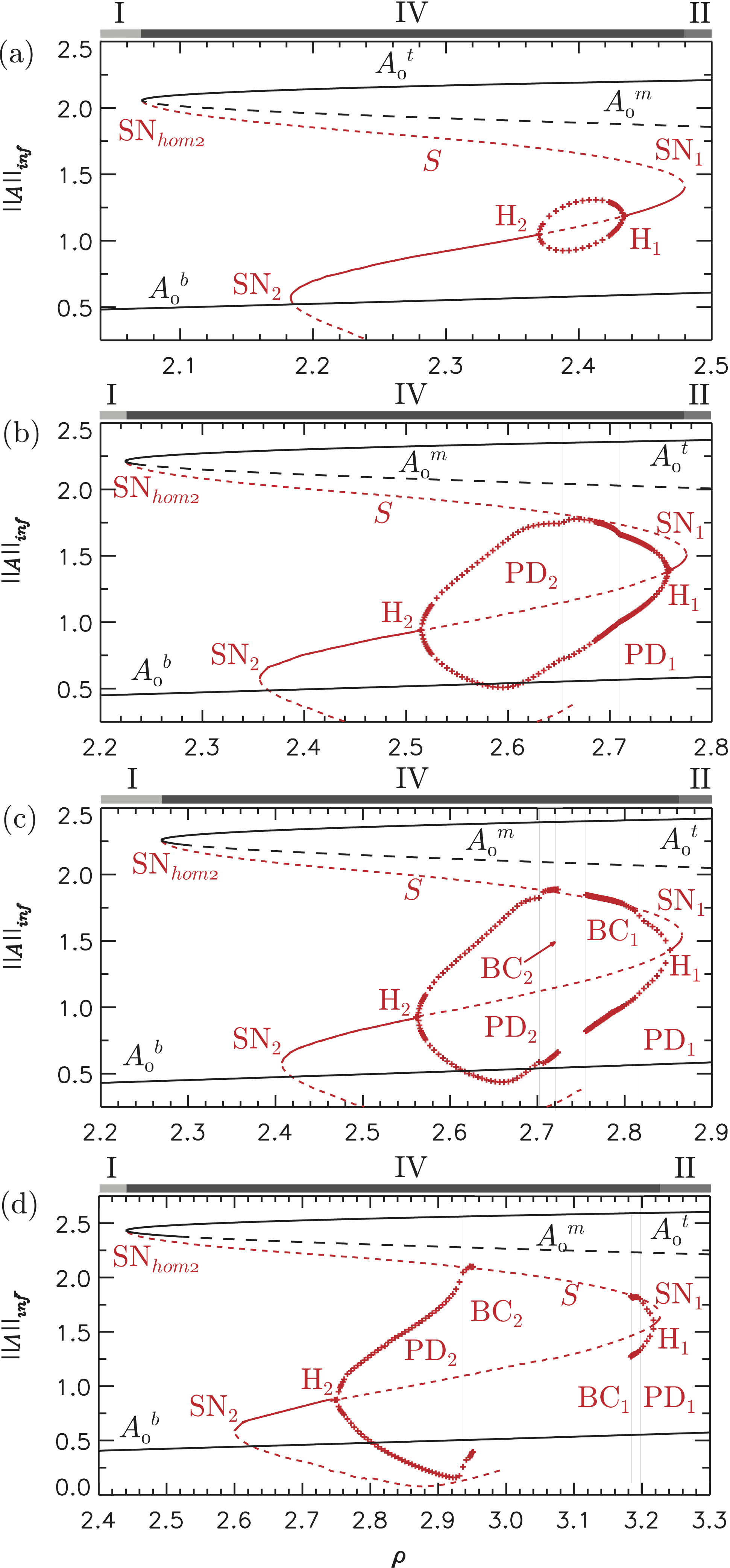
Figure 18: Bifurcation diagrams corresponding to different slices of the parameter space in Fig. 17 plotted using $||A||_{\rm inf}$ as a measure of the amplitude. Solid (dashed) lines correspond to stable (unstable) structures, and red (black) colors correspond to 1-SO dark DSs (HSS). The red crosses represent maxima and minima of the amplitude of the oscillatory dark DSs. The gray labeled bars above each panel show the extent of the regions I, II, and IV. (a) $\theta=4.6$, (b) $\theta=5$, (c) $\theta=5.2$, (d) $\theta=5.5$.

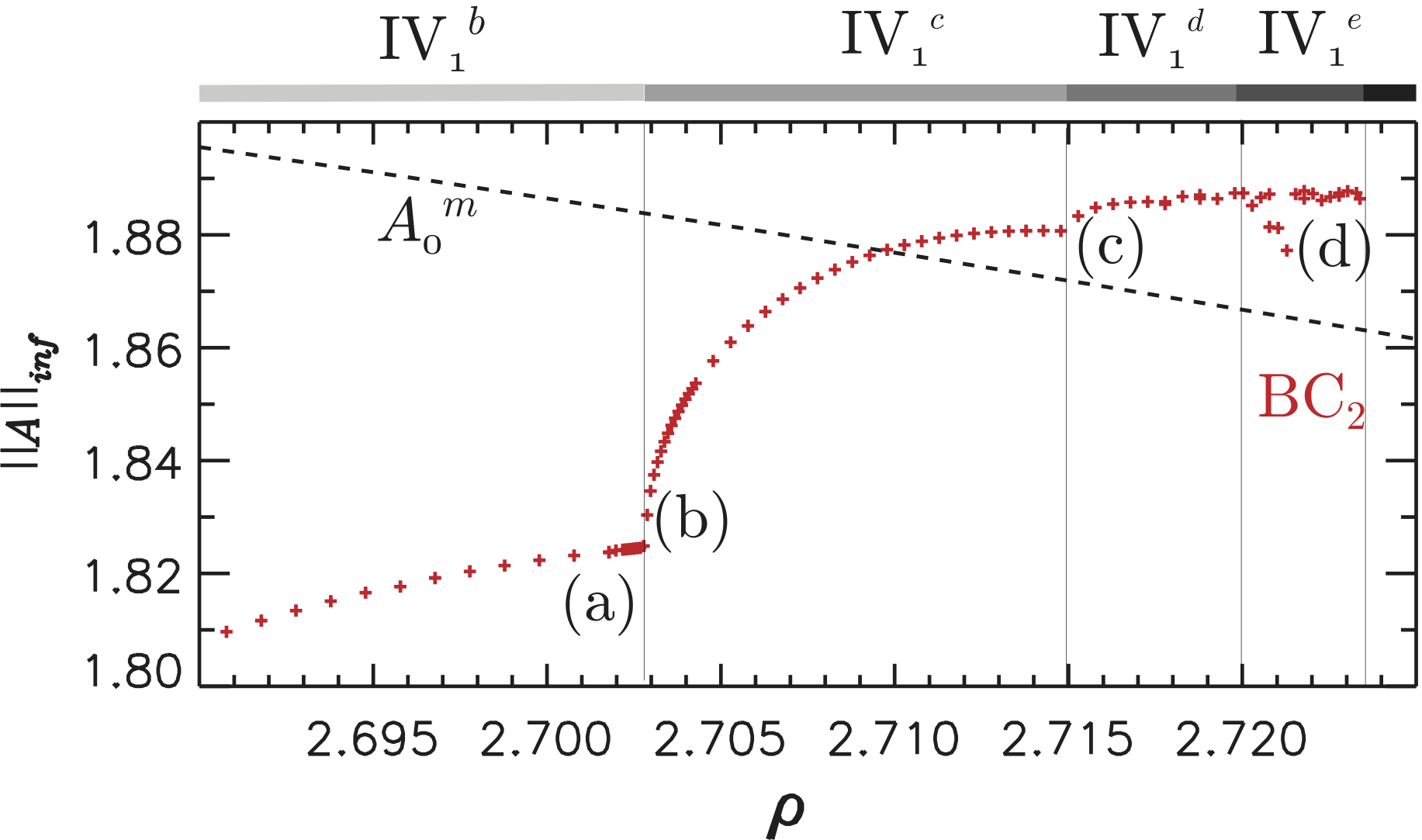
Figure 19: Detail of the bifurcation diagram of Fig. 18(c) for $\theta=5.2$ close to the BC₁ point. Vertical lines separate period 1 oscillations (region IV${}_{1}^{b}$), period 2 oscillations (region IV${}_{1}^{c}$), period 4 oscillations (region IV${}_{1}^{d}$) and temporal chaos in region IV${}_{1}^{e}$. Lines and markers in red (black) correspond to dark DSs (HSS). Labels from (a) to (d) correspond to the dynamics shown in Fig. 20.

Bifurcation lines separating different dynamical regimes are labeled according to Fig. 14. With increasing $\theta$ the Hopf bifurcation H${}^{-}_{1}$ of the single dark DS approaches SN₁ and we see that both lines are almost tangent although, for the parameter values presented, they do not meet. The same scenario repeats for the Hopf bifurcation H${}^{-}_{3}$ of the 2-SO state.

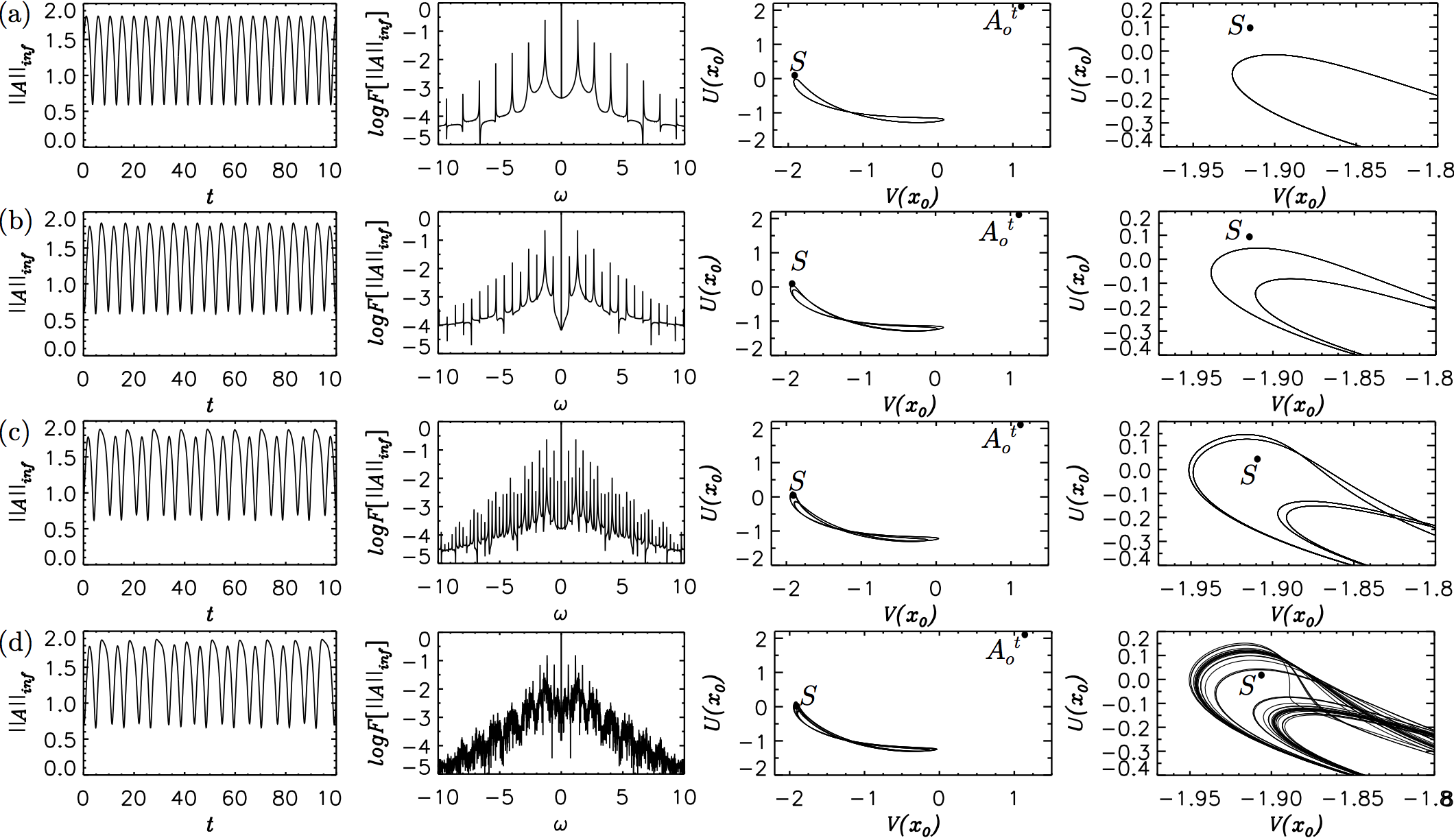
Figure 20: Route to temporal chaos for $\theta=5.2$. Panels (a)–(d) represent the transition from (a) period 1 oscillations to (d) temporal chaos, corresponding to the labels in Fig. 19. From left to right: temporal trace of $||A||_{\rm inf}$, its frequency spectrum that allows us to differentiate between the different types of temporal periodicity, a portion of the phase-space containing $A_{0}^{t}$, $S$ and the periodic attractors, and a zoom of the latter where we can appreciate the proximity of $S$ to the cycle. (a) $\rho=2.70248$ (period 1), (b) $\rho=2.70358$ (period 2), (c) $\rho=2.71528$ (period 4), (d) $\rho=2.72178$ (temporal chaos).

This scenario can be better understood by looking at Fig. 18 where several slices of Fig. 17 at different values of $\theta$ are shown. We choose to plot $||A||_{\inf}:={\rm min}(|A|)$ instead of the $L^{2}$ norm to improve the clarity of the bifurcation diagram, and denote the maximum and minimum amplitude of the oscillatory DSs using crosses. The diagram in Fig. 18(a) corresponds to a cut of Fig. 17 at $\theta=4.6$. At this $\theta$ value the oscillatory state bifurcates from H${}^{-}_{1}$, grows in amplitude as $\rho$ decreases, before reconnecting to the stationary DS at H${}^{-}_{2}$ in a reverse Hopf bifurcation. For larger $\theta$, the amplitude of the limit cycle between H${}^{-}_{1}$ and H${}^{-}_{2}$ increases, and at some point the cycle undergoes a period-doubling (PD) bifurcation, starting a route to a chaotic attractor. This happens already at $\theta=5$ as can be seen in Fig. 18(b). At $\theta=5.2$ (Fig. 18(c)) the chaotic attractor touches the saddle branch $S$ corresponding to unstable dark solitons and disappears through a boundary crisis (BC) Hilborn . Let us discuss this process in detail for the cycle emerging from H${}^{-}_{2}$ (the case of H${}^{-}_{1}$ is analogous). In Fig. 19 we show a zoom of the diagram in Fig. 18(c) close to BC₂ and in Fig. 20 a series of panels characterizing the cycle at different values of $\rho$ is shown. From left to right we show a series of time traces corresponding to the temporal evolution of the minima of the soliton, i.e., $||A||_{\inf}$, the Fourier transform of these time traces, a two-dimensional phase space projection onto $(U(x_{0},t),V(x_{0},t))$, $x_{0}$ being the position of the center of the structure, and a zoom of the phase space. Panel (a) in Fig. 20 corresponds to the situation at $\rho=2.70248$ in Fig. 19 labeled with (a). As we can see in the time trace and in the frequency spectrum, the cycle has a single period. In the phase space shown in Fig. 20 we observe a fixed point corresponding to $A_{0}^{t}$, a saddle point corresponding to the unstable dark soliton denoted by $S$ and a periodic orbit corresponding to the cycle. For this value of $\rho$ the saddle $S$ is far from the cycle. For $\rho=2.70358$ (panel (b) corresponding to label (b) in Fig. 19 the time trace and the spectrum reveal that the cycle has period two as can also be discerned from the phase space projection. In Fig. 20(c) for $\rho=2.71528$ the cycle has just suffered another period-doubling resulting a cycle with period four. Finally, Fig. 20(d) shows the situation for $\rho=2.72178$, where the cycle has become a chaotic attractor. At this parameter value the system is very close to the boundary crisis BC₂ as can appreciated from the near tangency between $S$ and the chaotic attractor. Once $S$ touches the attractor, the latter disappears and only $A^{t}_{0}$ and $A_{0}^{b}$ remain as attractors of the system. The same occurs to the cycles appearing at H${}^{-}_{1}$. Using time simulations we were able to estimate the position of the boundary crises BC₁ and BC₂ in parameter space, labeled in Fig. 17(a). From Fig. 18(c) to Fig. 18(d) we can see that at the same time as BC₁ moves toward H${}^{-}_{1}$, H${}^{-}_{1}$ itself approaches SN₁ and therefore that the region of existence of oscillatory DSs shrinks. This behavior can also be seen in Fig. 17(a).

At this point we can differentiate five main dynamical subregions related to region IV₁, i.e., the 1-SO dark soliton, namely:

• IV${}_{1}^{a}$: The 1-SO dark soliton is stable

• IV${}_{1}^{b}$: The soliton oscillates with a single period

• IV${}_{1}^{c}$: The soliton oscillates with period two

• IV${}_{1}^{d}$: The soliton oscillates with period four

• IV${}_{1}^{e}$: Region of temporal chaos bounded by a boundary crisis (BC₂).

The region IV₂ of 2-SO dark solitons has the same sequence of subregions IV${}_{2}^{a}$,…,IV${}_{2}^{e}$, etc.

Close to BC₂ (respectively, BC₁) the system can exhibit behavior reminiscent of excitability gomila . Here the stable manifold of the saddle soliton $S$ acts as a separatrix or threshold in the sense that perturbations of $A_{0}^{t}$ across that threshold do not relax immediately to $A^{t}_{0}$ but lead first to a large excursion in phase space before relaxing to $A_{0}^{t}$. In this case the excursion corresponds to what is known as a chaotic transient, where the system exhibits transient behavior reminiscent of the chaotic attractor at lower values of $\rho$ leo-lendert ; Ott . In Figs. 21(a) and (b) we show two examples of this kind of transient dynamics. We choose a value of $\rho$ close to BC₂, namely $\rho=2.7235$, and modify the parameter $\rho$ for a brief instant using a Gaussian profile of width $\sigma$ and height $h$ using the instantaneous transformation $\rho\mapsto\rho+h(t)\exp[-(x-L/2)^{2}/\sigma^{2}]$, where $\rho=2.7235$ and $\sigma=0.781250$ with $h(t)=-2.55$ for $10\leq t\leq 15$ and $h=0$ elsewhere Parra_Rivas_drift_defect . As shown in Fig. 21(a) such a perturbation of $A_{0}^{t}$ allows the system to explore the chaotic attractor before returning to the rest state. In contrast, in Fig. 21(b) the system explores just one loop of the cycle before returning to the rest state.

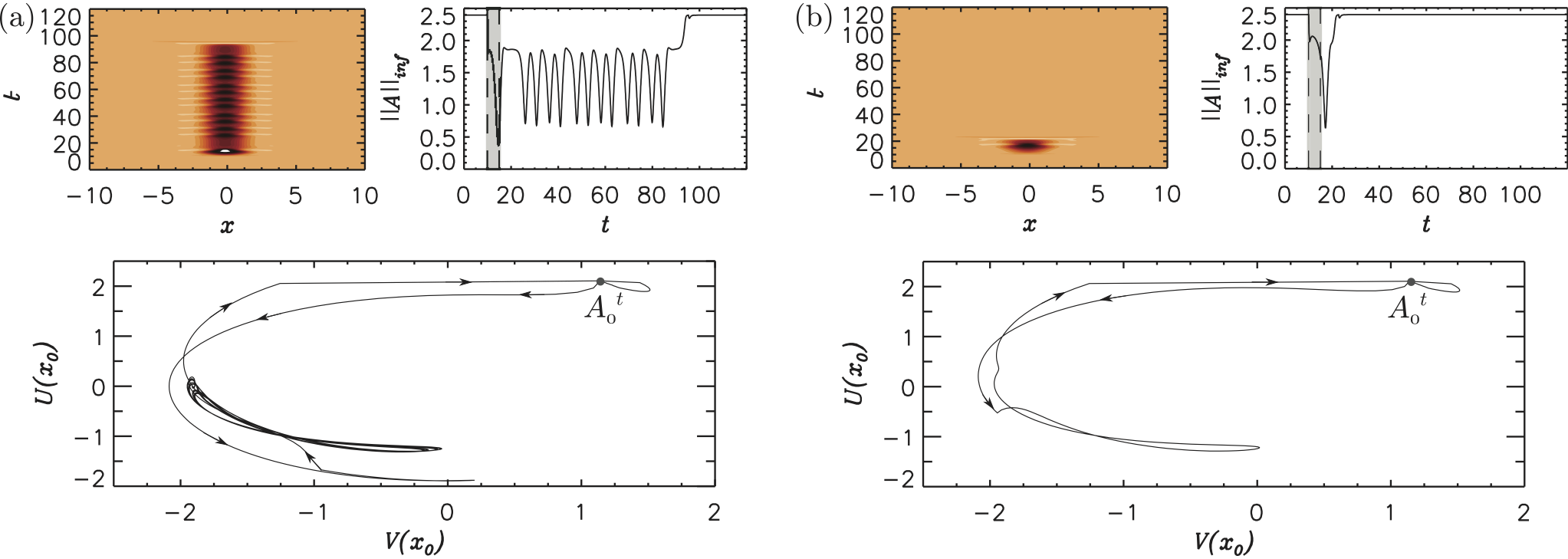
Figure 21: (Color online) Chaotic transient dynamics for $\theta=5.2$: (a) A chaotic transient is generated when $A_{0}^{t}$ is temporally perturbed with a Gaussian perturbation of height $h=-2.55$ (see gray area in time traces); (b) a similar excursion for $h=-3.4431$. In both (a) and (b) the top left panels represent space-time plots of the temporal evolution of the field $U(x,t)$, the top right panels show the time series of the norm $||A||_{\inf}$ and the bottom panels a projection of the phase space trajectory.

VI Concluding remarks

In this work we have presented a comprehensive overview of the dynamics of the LLE in the normal dispersion regime. The bifurcation structure of dark dissipative solitons (DSs), their stability and the regions of their existence were determined. Three families of dark solitons, the 1-soliton and two different types of 2-soliton states, located on three intertwined branches undergoing collapsed snaking in the vicinity of the same Maxwell point, were identified. The 1-soliton states bifurcate from the top left fold of an S-shaped branch of spatially homogeneous states and terminate either on the lower homogeneous steady state (HSS) branch in a Hamiltonian-Hopf (HH) (equivalently, modulational instability) or at the bottom right fold, depending on the detuning parameter $\theta$. On a periodic domain of finite spatial period, these bifurcations are slightly displaced from the folds, and in the case of the HH bifurcation to finite amplitude on the branch of periodic states created in this bifurcation. The 2-soliton states consisting of a pair of identical equidistant solitons in the domain follow a similar branch but branch off the HSS farther from the folds. This is a finite size effect: these states behave like the 1-soliton states on a periodic domain with half the domain length. The third branch consists of a pair of nonidentical solitons and plays a key role: this branch bifurcates from the branch of identical 2-soliton states in a pitchfork bifurcation; as one follows this branch to lower $L^{2}$ norm these states undergo a remarkable metamorphosis into a bright soliton with a minimum at its center that allows it to terminate on the periodic states created in the HH bifurcation at the same location as the 1-soliton states, as demanded by theory. The details of this transition are captured in Figs. 12 and 13.

At yet higher values of the detuning parameter $\theta$ we found that the localized states undergo oscillatory instabilities, and at a certain point a period-doubling bifurcation initiates a period-doubling cascade into chaos. We have used this observation to determine the regions in parameter space where different stationary and dynamical states coexist.

We have shown that the bifurcations that organize the spatial dynamics undergo an important transition at a Quadruple-Zero (QZ) point, which occurs at $(\theta,\rho)=(2,\sqrt{2})$. Here, in the normal dispersion regime, the Belyakov-Devaney (BD) transition turns into an HH bifurcation as the detuning $\theta$ increases through $\theta=2$. For $\theta>2$ a spatially periodic pattern bifurcates subcritically from the bottom homogeneous state at this HH bifurcation. These periodic solutions were found to be unstable, and hence no stable bright DSs were found. However, the saddle-node bifurcation of the top homogeneous solution remains a reversible Takens-Bogdanov (RTB) bifurcation for all $\theta>\sqrt{3}$. This observation explains the existence of multiple families of dark DSs in this regime, and their organization in the so-called collapsed snaking structure BuYoKn ; BuYoKn_colapsing . As mentioned, these dark DSs undergo various dynamical instabilities for larger values of the detuning $\theta$.

The bifurcation scenario is largely reversed in the case of anomalous dispersion, where the same QZ point plays an equally important role, but now the HH bifurcation turns into a BD bifurcation when $\theta>2$ Parra_Rivas_2 ; Goday_chembo . Moreover, the top homogeneous solution is now always unstable and the upper fold never corresponds to a RTB bifurcation. This reverse character of the bifurcation points has important consequences. First, dark DSs no longer exist, although the inclusion of additional, higher order dispersion can stabilize the top homogeneous solution and hence lead to stable DSs Gelens_darkDS . Second, for $41/30<\theta<2$, a stable periodic solution coexists with the stable bottom homogeneous solution giving rise to bright DSs that are organized in a homoclinic snaking structure gomila_Scroggi ; Champneys . For $\theta>2$, however, the snaking structure of such bright DSs breaks down, as will be reported elsewhere. Finally, despite these differences in the regions of existence of dark and bright DSs in the normal vs. anomalous dispersion regime, the temporal dynamics of the existing solutions are very similar at higher values of the detuning $\theta$. Here, for normal dispersion, we reported the existence of oscillatory and chaotic dynamics of dark DSs as the detuning is increased. The same dynamical instabilities have been observed in the case of anomalous dispersion at high values of $\theta$, but this time for bright DSs leo-lendert ; Parra_Rivas_2 . This suggests that the unfolding of the dynamics can be related to the same type of bifurcation point in both cases.

Owing to the strong correspondence between Kerr temporal solitons and frequency combs (FCs), the LLE has recently attracted renewed interest CS_KFC . FCs consist of a set of equidistant spectral lines that can be used to measure light frequencies and hence time intervals more easily and precisely than ever before combs . For this reason FCs open up a large variety of new applications ranging from optical clocks to astrophysics combs . We explore the consequences of the present analysis for FC technology in a companion paper KFC_dark .

As shown in Fig. 4, in the normal dispersion regime rather large values of the detuning $\theta$ and pump power $\rho$ are required to obtain a sufficiently wide region of dark DSs (region IV) to observe such states experimentally. However, in recent years, the FC community has become increasingly successful at reaching the required values of pump power and detuning. As a result, dark DSs with different numbers of spatial oscillations (SOs) in their center (see, e.g., Fig. 10) have been experimentally observed Xue_NP . In Ref. Xue_NP dark DSs were found using a normalized pump power $\rho\approx 2.5$ and normalized detuning $\theta\approx 5$. Figures 17 and 18 show that around these parameter values one can indeed find dark DSs with different numbers of SOs that can undergo oscillatory instabilities.

Our analysis provides a detailed map of the regions of existence and stability of dark DSs, which could serve as a guide for experimentalists to target particular DS solutions. We showed that dark DSs exist only in a well-defined zone within the wider region of bistability between two stable homogeneous solutions. Within this zone, dark DSs are organized in a bifurcation structure called a collapsed snaking structure. The word ”collapsed” refers to the fact that the region of existence of dark DSs shrinks exponentially with increasing number of SOs in the soliton profile (see Fig. 8). The collapse of the snaking structure implies that DSs with many SOs can only be found at the Maxwell point $\rho_{M}$, a fact that favors the observation of DSs with a single SO over that of broader DS with many SO.

Although such a collapsed snaking structure persists for higher values of the detuning $\theta$, we also showed that narrow dark DSs with a low number of SOs destabilize first as $\theta$ increases (Fig. 14) and start to oscillate in time. Therefore, at higher values of $\theta$ stable dark DSs found experimentally will most likely have an intermediate number of SOs. Our general analysis of the multistability of dark DSs can also explain previous numerical observations in Ref. Goday_chembo , where it was shown that the pulse profile of dark DSs becomes more distorted as the detuning increases. This could be due to the fact that stable dark DSs with a larger number of SOs are more likely to be found for higher values of the detuning.

Appendix

In this appendix we present details of the weakly nonlinear analysis near the RTB bifurcation at SN_hom,2 used to obtain analytically the spatially localized state in Eq. (19). These states are solutions of the ODE system defined by

$$\bigg{\{}\begin{array}[]{c}-\nu\displaystyle\frac{dV^{2}}{dx^{2}}-U+\theta V-V(U^{2}+V^{2})+\rho=0\\ \nu\displaystyle\frac{dU^{2}}{dx^{2}}-V-\theta U+U(U^{2}+V^{2})=0.\end{array}$$ (20)

The bifurcation SN_hom,2 takes place at

$$I_{t}=\displaystyle\frac{1}{3}(2\theta+\sqrt{\theta^{2}-3})$$ (21)

and we consider a Taylor series expansion of $\rho$ around $I_{t}$:

$$\rho(I_{0})=\underbrace{\rho(I_{t})}_{\rho_{t}}+\underbrace{\left(\frac{d\rho}{dI_{0}}\right)_{I_{t}}}_{=0}(I_{0}-I_{t})+\underbrace{\displaystyle\frac{1}{2}\left(\frac{d^{2}\rho}{dI^{2}_{0}}\right)_{I_{t}}}_{\delta}\underbrace{(I_{0}-I_{t})^{2}}_{\epsilon^{2}}+\cdots$$ (22)

with

$$\rho_{t}=\sqrt{I_{t}^{3}-2\theta I_{t}^{2}+(1+\theta^{2})I_{t}}.$$ (23)

Because $\rho_{t}$ has a minimum at $I_{t}$, we have

$$\left(\displaystyle\frac{d\rho}{dI_{0}}\right)_{I_{t}}=0$$

$$\delta=\displaystyle\frac{1}{2}\left(\displaystyle\frac{d^{2}\rho}{dI^{2}_{0}}\right)_{I_{t}}=\displaystyle\frac{\sqrt{\theta^{2}-3}}{2\rho_{t}}>0.$$

We define a small parameter $\epsilon$ in terms of $\rho$,

$$\epsilon=\sqrt{\frac{\rho-\rho_{t}}{\delta}},$$ (24)

and use $\epsilon$ as an expansion parameter.

The localized states of interest can be written in the form

$$\left[\begin{array}[]{c}U\\ V\end{array}\right]=\left[\begin{array}[]{c}U\\ V\end{array}\right]^{*}+\left[\begin{array}[]{c}u\\ v\end{array}\right],$$ (25)

with the spatially uniform states HSS given by

$$\left[\begin{array}[]{c}U\\ V\end{array}\right]^{*}=\left[\begin{array}[]{c}U_{t}\\ V_{t}\end{array}\right]+\epsilon\left[\begin{array}[]{c}U_{1}\\ V_{1}\end{array}\right]+\epsilon^{2}\left[\begin{array}[]{c}U_{2}\\ V_{2}\end{array}\right]+...$$ (26)

and the space-dependent terms by

$$\left[\begin{array}[]{c}u\\ v\end{array}\right]=\epsilon\left[\begin{array}[]{c}u_{1}\\ v_{1}\end{array}\right]+\epsilon^{2}\left[\begin{array}[]{c}u_{2}\\ v_{2}\end{array}\right]+...$$ (27)

We allow the fields $u_{1}$, $v_{1}$, $u_{2}$ and $v_{2}$ to depend on the slow variable $X\equiv\sqrt{\epsilon}x$. We first calculate the HSS terms and then do the same for the space-dependent terms.

Asymptotics for the uniform states

Inserting the ansatz (26) in Eq. (20), we obtain the correction to the HSS $A_{0}$ at any order in $\epsilon$.

At order $\mathcal{O}(\epsilon^{0})$ we obtain expressions for $U_{t}$ and $V_{t}$ as a function of $\theta$. At order $\mathcal{O}(\epsilon^{1})$ we have

$$L\left[\begin{array}[]{c}U_{1}\\ V_{1}\end{array}\right]=\left[\begin{array}[]{c}0\\ 0\end{array}\right],$$ (28)

where

$$L=\left[\begin{array}[]{cc}0&0\\ -(\theta-I_{t}-2U_{t}^{2})&-2\end{array}\right]$$ (29)

is a singular linear operator. Equation (28) has an infinite number of solutions that can be written in the form

$$\left[\begin{array}[]{c}U_{1}\\ V_{1}\end{array}\right]=\mu\left[\begin{array}[]{c}1\\ \eta\end{array}\right],$$ (30)

where

$$\eta=-\displaystyle\frac{1}{2}(\theta-I_{t}-2U_{t}^{2})$$ (31)

and $\mu$ is obtained by solving the $\mathcal{O}(\epsilon^{2})$ system. At this order we obtain the equation

$$L\left[\begin{array}[]{c}U_{2}\\ V_{2}\end{array}\right]=\left[\begin{array}[]{c}2U_{1}V_{1}U_{t}+(2V_{1}^{2}+I_{1})V_{t}-\delta\\ -(2U_{1}^{2}+I_{1})U_{t}-2V_{1}U_{1}V_{t}\end{array}\right],$$ (32)

where $I_{1}\equiv U_{1}^{2}+V_{1}^{2}$. Because $L$ is singular, the previous equation has no solution unless a solvability condition is satisfied. This condition is given by

$$\mu=\sqrt{\frac{\delta}{3\eta^{2}V_{t}+2\eta U_{t}+V_{t}}}.$$ (33)

Asymptotics for the space-dependent states

To calculate the space-dependent component of the weakly nonlinear state, we proceed in the same fashion. We insert the full ansatz for the asymptotic state, namely Eq. (25), into the system (20) and obtain, at order $\mathcal{O}(\epsilon^{1})$,

$$\underbrace{L\left[\begin{array}[]{c}U_{1}\\ V_{1}\end{array}\right]}_{=0}+L\left[\begin{array}[]{c}u_{1}\\ v_{1}\end{array}\right]=\left[\begin{array}[]{c}0\\ 0\end{array}\right],$$ (34)

where the first term on the LHS vanishes. The general solution of this equation is

$$\left[\begin{array}[]{c}u_{1}\\ v_{1}\end{array}\right]=\left[\begin{array}[]{c}U_{1}\\ V_{1}\end{array}\right]\psi(X),$$ (35)

with $\psi(X)$ a function to be determined at the next order.

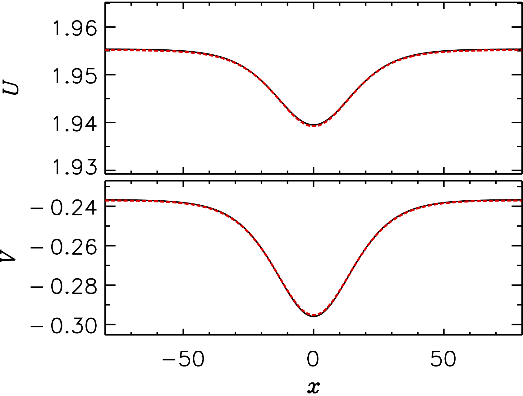
Figure 22: (Color online) Asymptotic and exact hole solutions $A(x)\equiv U(x)+iV(x)$ close to SN_hom,2 for $\theta=4$ and $\rho=1.98388$. The black solid line shows the asymptotic solution for comparison with the numerically exact solution obtained by numerical continuation (red dashed line). The two lines are indistinguishable.

At order $\mathcal{O}(\epsilon^{2})$

$$L\left[\begin{array}[]{c}u_{2}\\ v_{2}\end{array}\right]=-\mathcal{P}_{1}\left[\begin{array}[]{c}u_{1}\\ v_{1}\end{array}\right]-\mathcal{P}_{2}\left[\begin{array}[]{c}U_{t}\\ V_{t}\end{array}\right],$$ (36)

with the linear operators

$$\mathcal{P}_{1}=\left[\begin{array}[]{cc}-(2U_{t}V_{1}+2U_{1}V_{t})&-(\nu\partial_{X}^{2}+6V_{t}V_{1}+2U_{t}U_{1})\\ \nu\partial_{X}^{2}+6U_{t}U_{1}+2V_{t}V_{1}&2V_{t}U_{1}+2U_{t}V_{1}\end{array}\right]$$ (37)

and

$$\mathcal{P}_{2}=\left[\begin{array}[]{cc}-2v_{1}u_{1}&-(3v_{1}^{2}+u_{1}^{2})\\ 3u_{1}^{2}+v_{1}^{2}&2v_{1}u_{1}\end{array}\right].$$ (38)

Because $L$ is singular, Eq. (36) has no solution unless another solvability condition is satisfied. In the present case, this condition reads

$$\left[\begin{array}[]{cc}1&0\end{array}\right]\mathcal{P}_{1}\left[\begin{array}[]{c}u_{1}\\ v_{1}\end{array}\right]+\left[\begin{array}[]{cc}1&0\end{array}\right]\mathcal{P}_{2}\left[\begin{array}[]{c}U_{t}\\ V_{t}\end{array}\right]=0.$$ (39)

After some algebra, Eq. (39) reduces to an ordinary differential equation for $\psi(X)$,

$$\alpha_{1}\psi^{\prime\prime}(X)+\alpha_{2}\psi(X)+\alpha_{3}\psi^{2}(X)=0,$$ (40)

where

$$\begin{array}[]{ccc}\alpha_{1}=-\nu V_{1},&\alpha_{2}=-2\delta,&\alpha_{3}=-\delta.\end{array}$$ (41)

This equation has solutions homoclinic to $\psi=0$ given by

$$\psi(X)=-3\textnormal{sech}^{2}\left(\displaystyle\frac{1}{2}\sqrt{-\frac{\alpha_{2}}{\alpha_{1}}}(X-X_{0})\right),$$ (42)

representing a hole in the spatially uniform state located at $X=X_{0}$, hereafter at $X=0$. Since $X\equiv\sqrt{\epsilon}x$ and $\epsilon\equiv\sqrt{\displaystyle\frac{\rho-\rho_{t}}{\delta}}$ the corresponding first order spatial correction is given by

$$\left[\begin{array}[]{c}u_{1}\\ v_{1}\end{array}\right]=-3\mu\left[\begin{array}[]{c}1\\ \eta\end{array}\right]{\textnormal{sech}}^{2}\left[\displaystyle\frac{1}{2}\sqrt{-\frac{\alpha_{2}}{\alpha_{1}}}\left(\displaystyle\frac{\rho-\rho_{t}}{\delta}\right)^{1/4}x\right].$$ (43)

The resulting asymptotic solution for $\theta=4$ and $\rho=1.98388$ is shown in Fig. 22 (black solid lines). The corresponding numerically exact solution, obtained using numerical continuation, is shown in red dashed lines. The agreement is excellent.

For $\sqrt{3}<\theta<2$ the saddle node SN_hom,1 is also a RTB bifurcation and the same asymptotic calculation can therefore be used to compute the DSs present near this bifurcation. A related calculation can be used to compute the DS profiles near the point HH BuYoKn .

References

- (1) N. Akhmediev and A. Ankiewicz, eds., Dissipative Solitons, Lecture Notes in Physics 661 (Springer, New York, 2005); N. Akhmediev and A. Ankiewicz, eds., Dissipative Solitons: From Optics to Biology and Medicine, Lecture Notes in Physics 751 (Springer, New York, 2008).
- (2) J.E. Pearson, Science 261, 189 (1993); K.J. Lee, W.D. McCormick, Q. Ouyang, and H.L. Swinney, Science 261, 192 (1993).
- (3) I. Müller, E. Ammelt, and H.G. Purwins, Phys. Rev. Lett. 82, 3428 (1999).
- (4) O. Thual and S. Fauve, J. Phys. (France) 49, 1829 (1988)
- (5) W.A. Macfadyen, Geogr. J. 116, 199 (1950).
- (6) Feature Section on Cavity Solitons, edited by L.A. Lugiato, IEEE J. Quantum Electron. 39, 2 (2003); M. Tlidi, P. Mandel, and R. Lefever, Phys. Rev. Lett. 73, 640 (1994); B. Schäpers, M. Feldmann, T. Ackemann, and W. Lange, Phys. Rev. Lett. 85, 748 (2000); S. Barland, J.R. Tredicce, M. Brambilla, L.A. Lugiato, S. Balle, M. Giudici, T. Maggipinto, L. Spinelli, G. Tissoni, T. Knodl, M. Miller, and R. Jager, Nature (London) 419, 699 (2002); W.J. Firth and C.O. Weiss, Opt. Photonics News 13, 55 (2002); F. Pedaci, S. Barland, E. Caboche, P. Genevet, M. Giudici, J.R. Tredicce, T. Ackemann, A. Scroggie, W. Firth, G.L. Oppo, G. Tissoni, and R. Jaeger, Appl. Phys. Lett. 92, 011101 (2008); V. Odent, M. Taki, and E. Louvergneaux, New J. Phys. 13, 113026 (2011).
- (7) F. Leo, S. Coen, P. Kockaert, S.P. Gorza, P. Emplit, and M. Haelterman, Nature Photon. 4, 471 (2010).
- (8) L.A. Lugiato and R. Lefever, Phys. Rev. Lett. 58, 2209 (1987).
- (9) D. Gomila, A.J. Scroggie, and W.J. Firth, Phys. D (Amsterdam) 227, 70 (2007).
- (10) F. Leo, L. Gelens, P. Emplit, M. Haelterman, and S. Coen, Opt. Express 21, 9180 (2013).
- (11) P. Parra-Rivas, D. Gomila, M.A. Matías, S. Coen, and L. Gelens, Phys. Rev. A 89, 043813 (2014).
- (12) C. Godey, I.V. Balakireva, A. Coillet, and Y.K. Chembo, Phys. Rev. A 89, 063814 (2014).
- (13) X. Xue, Y. Xuan, Y. Liu, P.-H. Wang, S. Chen, J. Wang, D.E. Leaird, M. Qi, and A.M. Weiner, Nature Photon. 9, 594 (2015).
- (14) V.E. Lobanov, G. Lihachev, T.J. Kippenberg, and M.L. Gorodetsky, Opt. Expr. 23, 7713-7721 (2015).
- (15) P. Parra-Rivas, D. Gomila, E. Knobloch, S. Coen, and L. Gelens, arXiv:1602.07068.
- (16) M. Haelterman, S. Trillo, and S. Wabnitz, Opt. Comm. 91, 401 (1992).
- (17) J. Burke, A. Yochelis, and E. Knobloch, SIAM J. Appl. Dyn. Syst. 7, 651 (2008).
- (18) M. Haragus and G. Iooss, Local Bifurcations, Center Manifolds, and Normal Forms in Infinite-Dimensional Dynamical Systems (Springer, Berlin, 2011).
- (19) A.R. Champneys, Phys. D (Amsterdam) 112, 158 (1998).
- (20) P. Colet, M.A. Matías, L. Gelens, and D. Gomila, Phys. Rev. E 89, 012914 (2014); L. Gelens, M.A. Matías, D. Gomila, T. Dorissen, and P. Colet, Phys. Rev. E 89, 012915 (2014).
- (21) R. Devaney, Trans. Am. Math. Soc. 218, 89 (1976).
- (22) A.J. Homburg and B. Sandstede, in Handbook of Dynamical Systems, edited by B. Hasselblatt, H. Broer, and F. Takens (North Holland, Amsterdam, The Netherlands, 2010), Chap. 8, pp. 379–524.
- (23) E. Knobloch. Annu. Rev. Cond. Matter Phys. 6, 325 (2015).
- (24) G. Iooss and M.C. Pérouème J. Diff. Eqs., 102, 62 (1993).
- (25) K. Kolossovski, A.R. Champneys, A.V. Buryak, and R.A. Sammut, Phys. D (Amsterdam) 171, 153 (2002).
- (26) E.L. Allgower and K. Georg, Numerical Continuation Methods: An Introduction (Springer, Berlin, 1990).
- (27) J. Knobloch and T. Wagenknecht, Phys. D (Amsterdam) 206, 82 (2005).
- (28) Y.-P. Ma, J. Burke, and E. Knobloch, Phys. D (Amsterdam) 239, 1867 (2010).
- (29) A. Yochelis, J. Burke, and E. Knobloch, Phys. Rev. Lett. 97, 254501 (2006).
- (30) A.R. Champneys, E. Knobloch, Y.-P. Ma, and T. Wagenknecht, SIAM J. Appl. Dyn. Syst. 11, 1583 (2012).
- (31) R. Hilborn, Chaos and Nonlinear Dynamics: An introduction for Scientists and Engineers (Oxford University Press, Oxford, 2000).
- (32) D. Gomila, M.A. Matías, and P. Colet, Phys. Rev. Lett. 94, 063905 (2005); D. Gomila, A. Jacobo, M.A. Matías, and P. Colet, Phys. Rev. E 75, 026217 (2007).
- (33) C. Grebogi, E. Ott, and J.A. Yorke, Phys. D (Amsterdam) 7, 181 (1983).
- (34) P. Parra-Rivas, D. Gomila, M.A. Matías, and P. Colet, Phys. Rev. Lett. 110, 064103 (2013); P. Parra-Rivas, D. Gomila, M.A. Matías, P. Colet, and L. Gelens, Opt. Express 22, 3486 (2014); P. Parra-Rivas, D. Gomila, M.A. Matías, P. Colet, and L. Gelens, Phys. Rev. E 93, 012211 (2016).
- (35) M. Tlidi and L. Gelens, Opt. Lett. 35, 306 (2010); M. Tlidi, P. Kockaert, and L. Gelens, Phys. Rev. A 84, 013807 (2011).
- (36) S. Coen, H.G. Randle, T. Sylvestre, and M. Erkintalo, Opt. Lett. 38, 37 (2013); S. Coen and M. Erkintalo, Opt. Lett. 38, 1790 (2013); Y.K. Chembo and C.R. Menyuk, Phys. Rev. A 87, 053852 (2013).
- (37) P. Del’Haye, A. Schliesser, O. Arcizet, T. Wilken, R. Holzwarth, and T.J. Kippenberg, Nature (London) 450, 1214 (2007); S. Cundiff, J. Ye, and J. Hall, Sci. Am. 298, 74 (2008); T. J. Kippenberg, R. Holzwarth, and S. A. Diddams, Science 332, 555 (2011); Y. Okawachi, K. Saha, J. S. Levy, Y. H. Wen, M. Lipson, and A. L. Gaeta, Opt. Lett. 36, 3398 (2011); F. Ferdous, H. Miao, D. E. Leaird, K. Srinivasan, J. Wang, L. Chen, L. T. Varghese, and A. M. Weiner, Nature Photon. 5, 770 (2011); T. Herr, K. Hartinger, J. Riemensberger, C. Y. Wang, E. Gavartin, R. Holzwarth, M. L. Gorodetsky, and T. J. Kippenberg, Nature Photon. 6, 480 (2012); S. B. Papp, K. Beha, P. Del’Haye, F. Quinlan, H. Lee, K. J. Vahala, and S. A. Diddams, Optica 1, 10 (2014).