ExoMol molecular line lists - XIV: The rotation-vibration spectrum of hot SO₂

Abstract

Sulphur dioxide is well-known in the atmospheres of planets and satellites, where its presence is often associated with volcanism, and in circumstellar envelopes of young and evolved stars as well as the interstellar medium. This work presents a line list of 1.3 billion ³²S¹⁶O₂ vibration-rotation transitions computed using an empirically-adjusted potential energy surface and an ab initio dipole moment surface. The list gives complete coverage up to 8000 cm^-1 (wavelengths longer than 1.25 $\mu$m) for temperatures below 2000 K. Infrared absorption cross sections are recorded at 300 and 500 C are used to validated the resulting ExoAmes line list. The line list is made available in electronic form as supplementary data to this article and at www.exomol.com.

1 Introduction

Suphur dioxide, SO₂, has been detected in a variety of astrophysical settings. Within the solar system, SO₂ is known to be a major constituent of the atmospheres of Venus (Barker, 1979; Belyaev et al., 2012, 2008; Arney et al., 2014) and Jupiter’s moon, Io (Pearl et al., 1979; Nelson et al., 1980; Ballester et al., 1994). SO₂ has been observed in the atmosphere of Mars, although to a much lesser extent (Khayat et al., 2015a). Volcanic activity is an important indicator of the presence of SO₂.

The chemistry of sulphur-bearing species, including SO₂, has been studied in the atmospheres of giant planets, brown dwarfs, and dwarf stars by Visscher et al. (2006). SO₂ has been observed in circumstellar envelopes of young and evolved stars (Yamamura et al., 1999; van der Tak et al., 2003; Ziurys, 2006; Adande et al., 2013), and in molecular clouds and nebulae within the interstellar medium (Klisch et al., 1997; Schilke et al., 2001; Crockett et al., 2010; Belloche et al., 2013). Extragalactic detection of SO₂ has even been achieved (Martin et al., 2003, 2005), emphasising the universal abundance of this particular molecule.

SO₂ is known to occur naturally in Earth’s atmosphere where it is found in volcanic emissions and hot springs (Stoiber & Jepsen, 1973; Khayat et al., 2015b) where observation of gases such as SO₂ provide a useful tool in the understanding of such geological processes. The spectroscopic study of SO₂ can also provide insight into the history of the Earth’s atmosphere (Whitehill et al., 2013). However its most important impact is arguably through its contribution to the formation of acid rain (Hieta & Merimaa, 2014) where the oxidisation of SO₂ to SO₃ in the atmosphere, followed by subsequent rapid reaction with water vapour results in the production of sulphuric acid (H₂SO₄), which leads to many adverse environmental effects. Spectra of hot SO₂ are also important for technological applications such as monitoring engine exhausts (Voitsekhovskaya et al., 2013), combustion (Hieta & Merimaa, 2014) and etching plasmas (Greenberg & Hargis, 1990).

One of the most exciting astronomical developments in recent years is the discovery of extrasolar planets, or “exoplanets”. The observation of the tremendous variety of such bodies has challenged the current understanding of solar system and planetary formation. Exoplanet detection methods have grown in sophistication since the inception of the field, however efforts to characterise their atmospheres are relatively new (Tinetti et al., 2013). The well-documented distribution of sulphur oxides in various terrestrial and astrophysical environments means that a thorough understanding of their fundamental spectroscopic behaviour is essential in the future analysis of the spectra of these exoplanetary atmospheres, and of other bodies of interest observed through past, present and future space telescope missions (Huang et al., 2014; Kama et al., 2013).

Experimentally, SO₂ spectra have been studied in both the ultra-violet (Freeman et al., 1984; Stark et al., 1999; Rufus et al., 2003; Danielache et al., 2008; Lyons, 2008; Rufus et al., 2009; Blackie et al., 2011; Danielache et al., 2012; Franz et al., 2013; Endo et al., 2015) and infrared (Lafferty et al., 1992; Flaud & Lafferty, 1993; Lafferty et al., 1993, 1996; Chu et al., 1998; Henningsen et al., 2008; Ulenikov et al., 2009, 2010, 2011, 2012, 2013) at room-temperature; most of these data are captured in the HITRAN database (Rothman et al., 2013). Conversely, there is limited spectral data for SO₂ available at elevated temperatures, and much of it is either not applicable to the spectral region of interest or consists of remote observational data requiring a sophisticated, bespoke atmospheric model to be used in conjunction with a line list to reproduce it (Grosch et al., 2013; Khayat et al., 2015a). However a few measurements of cross section data have been made for hot SO₂ spectra in the laboratory by Grosch et al. (2013) and Grosch et al. (2015a). Here we extend this work by recording spectra of SO₂ in the infrared as a function of temperature for comparison with and validation of our computed line list.

Theoretically a number of studies have looked at the ultraviolet spectrum spectrum of SO₂ (Xie et al., 2000; Ran et al., 2007; Leveque et al., 2015) which represents a considerable challenge. More straightforward are studies of the vibration-rotation spectrum which lies in the infrared. Early work on this problem was performed by Kaupi & Halonen (1992) while recent work has focused on rotational excitation Kumar et al. (2015); Kumar & Poirier (2015). A number of comprehensive studies has been performed by the Ames group (Huang et al., 2014, 2015, 2016); this work provides an important precursor to this study and will be discussed further below.

The ExoMol project (Tennyson & Yurchenko, 2012) aims to provide molecular line lists for exoplanet and other atmospheres with a particular emphasis on hot species. Huang et al. (2014) used theoretical methods to compute a line list for SO₂ up to 8000 cm^-1 for a temperature of 296 K (denoted Ames-296K). This was recently extended to 5 isotopologues of SO₂ (Huang et al., 2015). This work and methodology follow closely similar studies on H₂O (Partridge & Schwenke, 1997), NH₃ (Huang et al., 2008, 2011a, 2011b), and CO₂ (Huang et al., 2012). In this work we build on the work of Huang et al. (2014) to compute a line list for hot SO₂ which should be appropriate for temperatures approaching 2000 K. Doing this required some technical adjustments both to the potential energy surface (PES) used and nuclear motion program employed; these are described in section 2. Section 3 presents our experimental work and section 4 the line list computations. Results and comparisons are given in section 5. Section 6 gives our conclusions.

2 Theoretical method

In order to compute a line list for SO₂ three things are required: a suitable potential energy surface (PES), dipole moment surface (DMS), and a nuclear motion program (Lodi & Tennyson, 2010). The DMS used here is the ab initio one of Huang et al. (2014) and is based on 3638 CCSD(T)/aug-cc-pV(Q+d)Z level calculations. The other parts are consider in the following subsections.

2.1 Potential Energy Surface

The Ames-1B PES used here is spectroscopically determined by refining an ab initio PES using room-temperature spectroscopic data. The Ames-1B PES refinement procedure used is very similar to the Ames-1 refinement reported by Huang et al. (2014). The two main differences are the choice of the initial PES and the use of a now-converged stretching basis. The published Ames-1 PES was chosen as the initial PES to adjust. All 22 zeroth- to fourth-order coefficients of the short-range PES terms are allowed to vary although the zeroeth-order constant does not affect the results. The number of reliable HITRAN (Rothman et al., 2013) energy levels included with $J=0/4/20/50/70$ are 23/43/183/181/129, respectively. The corresponding weights adopted for most levels are 2.5/1.0/1.5/2.0/3.0, respectively. For the original Ames-1 PES coefficients, the initial root mean square fit error, $\sigma_{\rm rms}$, are 0.175 cm^-1 (weighted) and 0.085 cm^-1 (unweighted). The refined coefficient set significantly reduces $\sigma_{\rm rms}$ to 0.028 cm^-1 (weighted) and 0.012 cm^-1 (unweighted). The PES is expressed in changes from equilibrium values of the bond lengths ($\Delta r_{1},\Delta r_{2}$) and bond angle ($\Delta\alpha$). Compared to the Ames-1 PES coefficients, the largest percentage variations are $\pm 11-22$% found for the following short-term expansion terms: $\Delta\alpha$ gradient, $\Delta r$ gradient, $\Delta r(\Delta\alpha)^{3}$, $\Delta r_{1}\Delta r_{2}$, $(\Delta r)^{2}(\Delta\alpha)^{2}$ and $(\Delta r_{1})^{3}\Delta r_{2}$, The changes in absolute value are largest for $(\Delta r_{1})^{2}\Delta\alpha\Delta r_{2}$ and $(\Delta r_{1})^{2}(\Delta r_{2})^{2}$. The Ames-1B PES has been used in recent SO₂ isotopologue calculations (Huang et al., 2016) and is available upon request.

The accuracy of the mass-independent Ames-1B PES remains approximately the same as the Ames-1 PES: about 0.01 cm^-1 for the three vibrational fundamentals of the three main isotopologues, 646, 828 and 628 in HITRAN notation, which therefore we can expect similar accuracy for the fundamentals of the minor isotopologues 636, 627 and 727 (Huang et al., 2016). For vibrational states as high as 5500 cm^-1, e.g. $5\nu_{1}$, accuracy for isotopologues using the Ames-1B PES should be better than 0.05 cm^-1. For those energy levels far beyond the upper limit included in our empirical refinement, e.g. 8000 – 10,000 cm^-1 and above, the accuracy would gradually degrade to a few wavenumbers, approximately the quality of the original ab initio PES before empirical refinement. The agreement between VTET and DVR3D results is better than 0.01 cm^-1 up to at least 8000 cm^-1. However, it should be noted that the Ames-1B PES was refined using the VTET program in such a way that although less than 500 HITRAN levels were adopted in the refinement, the accuracy is consistently as good as 0.01 – 0.02 cm^-1 from 0 to 5000 cm^-1. The accuracy mainly depends on the energy range covered by the refinement dataset, but not on whether a particular energy level was included in the refinement. Recent experiments have verified the prediction accuracy for non-HITRAN energy levels and bands. New experimental data at a higher energy range may significantly extend the wavenumber range with an 0.01 – 0.02 cm^-1 accuracy, provided a new refinement is performed with the new data. Currently, the accuracy of the reported line list is best at 296 K and below 7000 cm^-1. Higher energy levels may have errors ranging from 0.5 cm^-1 to a few cm^-1.

Use of the Ames-1B PES with the VTET nuclear motion program (Schwenke, 1996) employed by the Ames group and DVR3D (Tennyson et al., 2004) employed here gives very similar results for room temperature spectra. However, one further adjustment was required for high $J$ calculations as the PES appears to become negative at very small ${\rm H\hat{S}H}$ angles. Similar problems have been encountered before with water potentials (Choi & Light, 1992; Partridge & Schwenke, 1997; Shirin et al., 2003) which have been overcome by adding a repulsive H – H term to the PES. Here we used a slightly different approach. The bisector-embedding implementation in DVR3D has the facility to omit low-angle points from the calculation (Tennyson & Sutcliffe, 1992); usually only a few automatically-chosen points are omitted. An amendment to module DVR3DRJZ allowed for the selection of the appropriate PES region by omitting all low-angle functions beyond a user-specified DVR grid point. This amendment was essential for the high $J$ calculations. This version of the code was used for all calculations with $J\geq$ 50 pressented. For $J<$ 50 this defect only affected very high rovibrational energies computed in ROTLEV3B and there has no significant effect on the results.

2.2 Nuclear motion calculations

The line list was produced using the DVR3D program suite (Tennyson et al., 2004) and involved rotationally excited states up to $J=165$. As this doubled the highest $J$ value previously computed using DVR3D, a number of adjustments were necessary compared to the published version of the code.

Firstly, the improved rotational Hamiltonian construction algorithm implemented by Azzam et al. (2016) was employed; this proved vital to making the calculations tractable. Secondly, it was necessary to adjust the automated algorithm which generates (associated) Gauss-Legendre quadarature points and weigths: the previous algorithm failed for grids of more than 90 points but a simple brute-force search for zeroes in the associated Legendre $P_{N}^{k}(x)$ was found to work well for all $N$ and $k$ values tested ($N\leq 150$). Thirdly, the DVR3D algorithm relies on solving a Coriolis-decoupled vibrational problem for each $(J,k)$, where $k$ is the projection of the rotational motion quantum number, $J$, onto the chosen body-fixed $z$ axis. This provides a basis set from which functions used to solve the fully-coupled rovibrational problem are selected on energy grounds Sutcliffe et al. (1988). Our calculations showed that for $k$ values above 130 no functions were selected so an option was implemented in which only $(J,k)$ combinations which contributed functions were actually considered. This update does not save significant computer time, since the initial $(J,k)$ calculations are quick, but does reduce disk usage which also proved to be a significant issue in the calculations. Finally, it was found that algorithm used in module DIPOLE3 to read in the wavefunctions led to significant input/output problems. This module was re-written to reduce the number of times these wavefunctions needed to be read. The updated version of the DVR3D suite is available in the DVR3D project section of the CCPForge program depository (https://ccpforge.cse.rl.ac.uk/).

DVR3D calculations were performed in Radau coordinates using the so-called bisector embedding (Tennyson & Sutcliffe, 1992) which places the body-fixed axis close to standard A principle axis of SO₂ meaning the $k$ used by the program is close to the standard asymmetric top approximate quantum number $K_{a}$. The DVR (discrete variable representation) calculations are based on grid points corresponding to Morse oscillator-like functions (Tennyson & Sutcliffe, 1982) for the stretches and (associated) Legendre polynomials for the bend.

The rotational step in the calculation selects the lowest $n(J+1)$ functions from the $(J,k)$-dependent vibrational functions on energy grounds where $n$ is parameter which was chosen to converge the rotational energy levels. For $J<100$ it was found that $n=725$ was required to get good convergence. However such calculations become computationally expensive for high $J$ values for which, in practice, fewer levels are required. Reducing the value of $n$ to 500 was found to have essentially no effect on the convergence of rovibrational eigenvalues produced at $J$ = 124. For $J=124$, there are a total of 14 523 eigenvalues below 15 000 cm^-1 summed over all rotational symmetries. This constitutes roughly 8% of the total combined matrix dimension of 175 450 for $n$ = 725 and 12% of 121 000 for $n$ = 500. The value $n$ = 725 was originally obtained for convergence of energies at $J$ = 60, where the number of eigenvalues below 15 000 cm^-1 accounts for 38% of the combined matrix dimension of 88 450. The higher energies at $J$ = 60 are much more sensitive to the value of $n$ due to the way the basis functions are distributed, whereas for $J\geq$ 120 the energies below the 15 000 cm^-1 threshold are already easily converged at lower values of $n$. It was therefore decided to reduce $n$ to 500 for $J\geq 124$ which leads to minimal loss of accuracy.

Convergence of rovibrational energy levels with $n=725$ was obtained using $J=60$ calculations. The sum of energies below 10 000, 11 000, 12 000, 13 000, 14 000, and 15000 cm^-1 was used to give an indication of the convergence below those levels (see Table 3.1 in Underwood (2016) Thesis]). $J=60$ coincides with the largest number of ro-vibrational energies lying below 15 000 cm^-1, and thus the higher energies here are the most sensitive to the convergence tests. The value $n=725$ ensures that the sum of all energies below 10 000 cm^-1 and 15 000 cm^-1 are fully converged to within 0.0001 cm^-1 and to 1 cm^-1, respectively. Computed DVR3D rovibrational energies above 10 000 cm^-1, though converged, can not be guaranteed to be spectroscopically accurate, and are entirely dependent on the quality of the PES. This may have minor repercussions on the convergence of the partition function at the high end of the temperature range. Table 1 summarises the parameters used in the DVR3D calculations while Table 2 compares vibrational term values computed with DVR3D and VTET.

Table 1: Input parameters for DVR3DRJZ and ROTLEV3B modules of DVR3D (Tennyson et al., 2004).

DVR3DRJZ
Parameter	Value	Description
NPNT2	30	No. of radial DVR points (Gauss-Laguerre)
NALF	130	No. of angular DVR points (Gauss-Legendre)
NEVAL	1000	No. of eigenvalues/eigenvectors required
MAX3D	3052	Dimension of final vibrational Hamiltonian
XMASS (S)	31.963294 Da	Mass of sulphur atom
XMASS (O)	15.990526 Da	Mass of oxygen atom
$r_{e}$	3.0 a0	Morse parameter (radial basis funciton)
$D_{e}$	0.4 Eh	Morse parameter (radial basis funciton)
$\omega_{e}$	0.005 a.u.	Morse parameter (radial basis funciton)
ROTLEV3B
Parameter	Value	Description
NVIB	1000	No. of vib. functions read fot each $k$
$n$	725	Defines $IBASS=n(J+1)$ for $J<$ 124
$n$	500	Defines $IBASS=n(J+1)$ for $J\geq$ 124

Table 2: A comparison of even symmetry vibrational bands in cm^-1 based on the AMES-1B PES.

Band	VTET	DVR3D	Difference
$\nu_{2}$	517.8725	517.8726	-0.0001
$2\nu_{2}$	1035.1186	1035.1188	-0.0002
$\nu_{1}$	1151.7138	1151.7143	-0.0005
$3\nu_{2}$	1551.7595	1551.7598	-0.0003
$\nu_{1}+\nu_{2}$	1666.3284	1666.3288	-0.0004
$4\nu_{2}$	2067.8084	2067.8087	-0.0003
$\nu_{1}+2\nu_{2}$	2180.3187	2180.3191	-0.0004
$2\nu_{1}$	2295.8152	2295.8158	-0.0006
$5\nu_{2}$	2583.2704	2583.2708	-0.0004
$\nu_{1}+3\nu_{2}$	2693.7053	2693.7056	-0.0003
$2\nu_{3}$	2713.3936	2713.3938	-0.0002
$2\nu_{1}+\nu_{2}$	2807.1739	2807.1744	-0.0005
$6\nu_{2}$	3098.1428	3098.1432	-0.0004
$\nu_{1}+4\nu_{2}$	3206.5009	3206.5012	-0.0003
$\nu_{2}+2\nu_{3}$	3222.9523	3222.9526	-0.0003
$2\nu_{1}+2\nu_{2}$	3317.9078	3317.9082	-0.0004
$3\nu_{1}$	3432.2724	3432.2729	-0.0005
$7\nu_{2}$	3612.4145	3612.4150	-0.0005
$\nu_{1}+5\nu_{2}$	3718.7109	3718.7111	-0.0002
$2\nu_{2}+2\nu_{3}$	3731.9370	3731.9373	-0.0003
$2\nu_{2}+3\nu_{2}$	3828.0367	3828.0370	-0.0003
$\nu_{1}+2\nu_{3}$	3837.6154	3837.6161	-0.0007
$3\nu_{1}+\nu_{2}$	3940.3781	3940.3786	-0.0005
$8\nu_{2}$	4126.0668	4126.0673	-0.0005
$\nu_{1}+6\nu_{2}$	4230.3325	4230.3327	-0.0002
$3\nu_{2}+2\nu_{3}$	4240.3549	4240.3553	-0.0004
$2\nu_{1}+4\nu_{2}$	4337.5726	4337.5729	-0.0003
$\nu_{1}+\nu_{2}+2\nu_{3}$	4343.8153	4343.8158	-0.0005
$3\nu_{1}+2\nu_{2}$	4447.8567	4447.8572	-0.0005
$4\nu_{1}$	4561.0634	4561.0638	-0.0004
$9\nu_{2}$	4639.0726	4639.0731	-0.0005
$\nu_{1}+7\nu_{2}$	4741.3554	4741.3556	-0.0002
$4\nu_{2}+2\nu_{3}$	4748.2069	4748.2074	-0.0005
$2\nu_{1}+5\nu_{2}$	4846.5190	4846.5192	-0.0002
$\nu_{1}+2\nu_{2}+2\nu_{3}$	4849.4433	4849.4438	-0.0005
$2\nu_{1}+2\nu_{3}$	4953.5971	4953.5978	-0.0007
$3\nu_{1}+3\nu_{2}$	4954.7285	4954.7289	-0.0004
$4\nu_{1}+\nu_{2}$	5065.9188	5065.9192	-0.0004
$10\nu_{2}$	5151.3969	5151.3974	-0.0005

3 Line list calculations

Calculations were performed on the High Performance Computing Service Darwin cluster, located in Cambridge, UK. Each job from DVR3DRJZ, ROTLEV3B and DIPOLE3 is submitted to a single computing node consisting of two 2.60 GHz 8-core Intel Sandy Bridge E5-2670 processors, therefore making use of a total of 16 CPUs each through OpenMP parallelisation of the various BLAS routines in each module. A maximum of 36 hours and 64 Gb of RAM are available for each calculation on a node. The DVR3DRJZ runs generally did not require more than 2 hours of wall clock time. The most computationally demanding parts of the line list calculation are in ROTLEV3B for the diagonalisation of the Hamiltonian matrices, where wall clock time increases rapidly with increasing $J$. Matrix diagonalisation in all cases was performed using the LAPACK routine DSYEV (Anderson et al., 1999).

The calculations considered all levels with $J\leq$ 165 and energies below 15 000 cm^-1. This gave a total of 3 255 954 energy levels. Einstein-A coefficients were computed for all allowed transitions linking any energy level below 8000 cm^-1 with any level below 15 000 cm^-1. The parameters $J\leq 165$ and $E_{\rm low}=8000$ cm^-1 determine the upper temperature for which the line list is complete; the upper energy cut-off of 15 000 cm^-1 means that this line list is complete for all transitions longwards of 1.25 $\mu$m. In practice, the rotation-vibration spectrum of SO₂ is very weak at wavelengths shorter than this and can therefore safely be neglected. In the line list, known as ExoAmes, contains a total of 1.3 billion Einstein-A coefficients.

The partition function can be used to assess the completeness of the line list as a function of temperature, $T$ (Neale et al., 1996). The value of the partition function at $T$ = 296 K, computed using all our energy levels is 6337.131. With a cut-off of $J\leq$ 80, as used by Huang et al. (2014), the value for the same temperature is computed as 6336.803, which is in excellent agreement with their calculated value of 6336.789. Figure 1 shows the partition function values as a function of a $J$ cut-off for a range of $T$. The highest value of $J$ considered, $J$ = 165, defines the last point where the lowest energy is less than 8000 cm^-1, which is used as the maximum value of lower energy states in DIPOLE3 calculations. As can be seen from this figure, the partition function is well converged for $J$ = 165 at all temperatures.

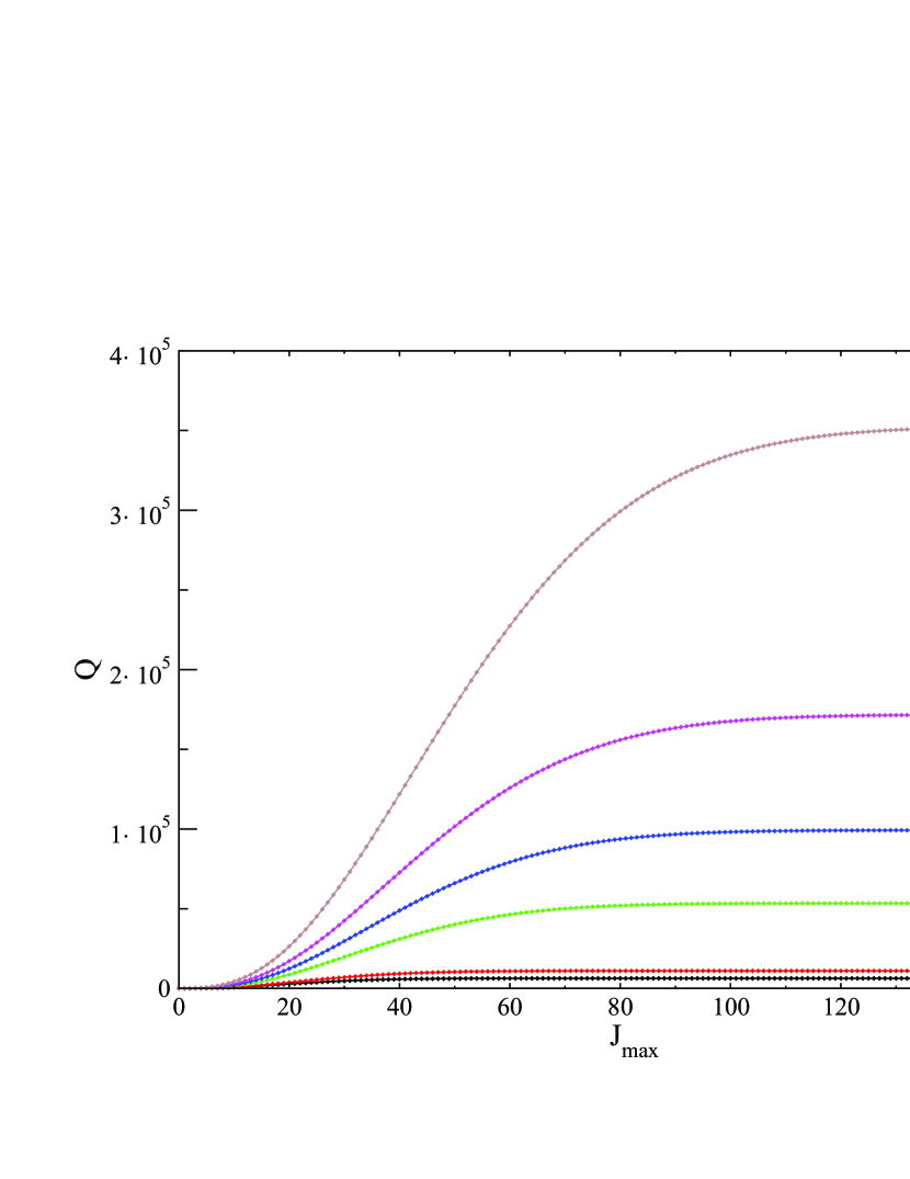
Figure 1: Convergence of partition function at different temperatures as a function of $J_{\rm max}$. The partition function increases monotonically with temperature.

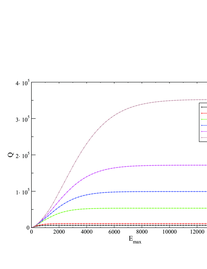
Figure 2: Convergence of partition function at different temperatures as a function of $E_{\rm max}$ (cm^-1). The partition function increases monotonically with temperature.

The $J$-dependent convergence of $Q$ gives a good indication of the completeness of the computed energy levels with respect to their significance at each temperature. However in order to ascertain the reliability of the line list for increasing temperatures it is more pertinent to observe the convergence of $Q$ as a function of energy cut-off; this is illustrated in Figure 2. The importance of this lies in the fact that the computed line list in the current work only considers transitions from energy levels below 8000 cm^-1. Since the physical interpretation of an energy level’s contribution to $Q$ is the probability of it’s occupancy, the completeness of the line list can only be guaranteed if all transitions from states with non-negligible population are computed. In other words, the line list may only be considered 100 % complete if $Q$ is converged when summing over all $E\leq$ 8000 cm^-1.

Figure 2 shows that, at a cut-off of 8000 cm^-1, the partition function is not fully converged for $T$ = 1500 K. Despite computing all rovibrational levels below 8000 cm^-1 ($J\leq$ 165), and all transitions from these states to states with $E\leq$ 15 000 cm^-1, there is still a minor contribution from energies above this cut-off to the partition sum, corresponding to all values of $J$. However, the neglected transitions are expected to make only a small additional contribution to the overall intensity at this temperature. The completeness of the line list may be quantified by considering the ratio of the partition function at the 8000 cm^-1 cut-off and the total partition function, $Q_{\rm Total}$, which takes into account all computed energies. Figure 3 shows this ratio as a function of temperature.

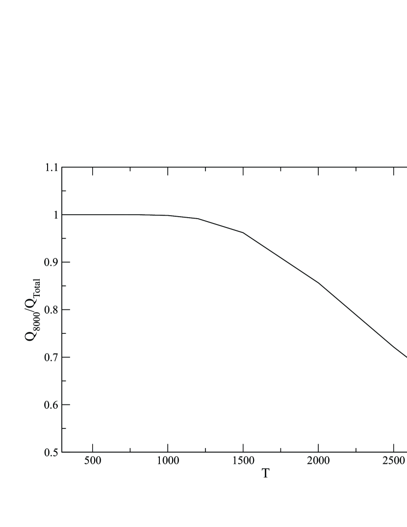
Figure 3: Ratios of $Q_{8000}$ to the assumed converged values $Q_{\rm Total}$ as a function of temperature.

For $T\leq$ 1500 K the line list is over 96 % complete. As can be seen from Figure 3 the level of completeness decreases with increasing temperature; at 2000 K the ratio falls to 86 %, and as low as 33 % for 5000 K. These values assume that $Q_{\rm Total}$ is equal to the ‘true’ value of the partition function and tests suggest that for $T=3000-5000$ K, the partition function is still converged to within 0.1 % when all computed energy levels are taken into consideration.

Table 3: Extract from the state file for SO₂. The full table is available from http://cdsarc.u-strasbg.fr/cgi-bin/VizieR?-source=J/MNRAS/xxx/yy.

$i$	$\tilde{E}$	$g$	$J$	$p$	$\nu_{1}$	$\nu_{2}$	$\nu_{3}$	$K_{a}$	$K_{c}$
1	0.000000	1	0	0	0	0	0	0	0
2	517.872609	1	0	0	0	1	0	0	0
3	1035.118794	1	0	0	0	2	0	0	0
4	1151.714304	1	0	0	1	0	0	0	0
5	1551.759779	1	0	0	0	3	0	0	0
6	1666.328818	1	0	0	1	1	0	0	0
7	2067.808741	1	0	0	0	4	0	0	0
8	2180.319086	1	0	0	1	2	0	0	0
9	2295.815835	1	0	0	2	0	0	0	0
10	2583.270841	1	0	0	0	5	0	0	0
11	2693.705600	1	0	0	0	4	0	0	0
12	2713.393783	1	0	0	0	0	2	0	0
13	2807.174418	1	0	0	2	1	0	0	0
14	3098.143224	1	0	0	0	6	0	0	0
15	3206.501197	1	0	0	0	5	0	0	0
16	3222.952550	1	0	0	0	1	2	0	0
17	3317.908237	1	0	0	1	3	0	0	0
18	3432.272904	1	0	0	3	0	0	0	0
19	3612.415017	1	0	0	0	7	0	0	0
20	3718.711074	1	0	0	0	6	0	0	0

$i$: State counting number.

$\tilde{E}$: State energy in cm^-1.

$g$: State degeneracy.

$J$: Total angular momentum

$p$: Total parity given by $(-1)^{J+p}$.

$\nu_{1}$: Symmetric stretch quantum number.

$\nu_{2}$: Bending quantum number.

$\nu_{3}$: Asymmetric stretch quantum number.

$K_{a}$: Asymmetric top quantum number.

$K_{c}$: Asymmetric top quantum number.

Table 3 gives a portion of the SO₂ states file. As DVR3D does not provide approximate quantum numbers, $K_{a}$, $K_{c}$ and the vibrational labels $\nu_{1}$, $\nu_{2}$ and $\nu_{3}$, these have been taken from the calculations of Huang et al. (2014), where possible, by matching $J$, parity and energy; these quantum numbers are approximate and may be updated in future as better estimates become available. Table 4 gives a portion of the transitions file. This file contains 1.3 billion transitions and has been split into smaller files for ease of downloading.

Table 4: Extract from the transitions file for SO₂. The full table is available from http://cdsarc.u-strasbg.fr/cgi-bin/VizieR?-source=J/MNRAS/xxx/yy.

$f$	$i$	A
679	63	1.9408E-13
36	632	5.6747E-13
42	643	1.7869E-11
635	38	1.1554E-11
54	662	3.6097E-11
646	44	1.9333E-08
660	52	2.5948E-08
738	98	3.4273E-06
688	69	3.4316E-06
47	650	1.4537E-11
648	45	3.4352E-06
711	82	3.5730E-06
665	55	3.5751E-06
716	85	3.4635E-06
670	58	3.4664E-06
635	37	3.4690E-06
611	23	3.4701E-06
595	12	3.4709E-06
734	95	3.7253E-06
684	66	3.7257E-06

$f$: Upper state counting number; $i$: Lower state counting number; $A_{fi}$: Einstein-A coefficient in s^-1.

4 Experiments

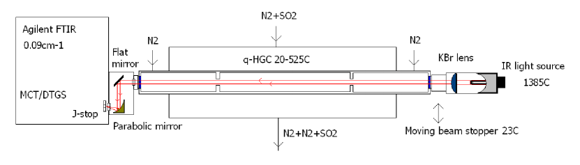
Figure 4: Optical set up used in the SO₂ infrared absorption measurements.

Experiments were performed at the Technical University of Denmark (DTU). Absorbance measurements for SO₂ were performed for temperatures up to 500 C using a quartz high-temperature gas flow cell (q-HGC). This cell is described in details by Grosch et al. (2013) and has recently been used for measurements of hot NH₃ (Barton et al., 2015), sulphur-containing gases (Grosch et al., 2015b) and some PAH compounds (Grosch et al., 2015c). The optical set-up is shown in Fig. 4. The set-up includes a high-resolution Fourier transform infraread (FTIR) spectrometer (Agilent 660 with a linearized MCT and DTGS detectors), the q-HGC and a light-source (Hawkeye, IR-Si217, 1385C) with a KBr plano-convex lens. The light source is placed in the focus of the KBr lens. The FTIR and sections between the FTIR/q-GHC and q-HGC/IR light source were purged using CO₂/H₂O-free air obtained from a purge generator. Bottles with premixed gas mixture, N₂ + SO₂ (5000 ppm) (Strandmøllen) and N₂ (99.998%) (AGA) were used for reference and SO₂ absorbance measurements. Three calibrated mass-flow controllers (Bronkhorst) were used to balance flow in the middle (N₂+SO₂) and the two buffer (N₂) parts on the q-HGC and to make additional dilution of the SO₂ to lower concentrations.

SO₂ absorbance measurements were performed at 0.25 – 0.5 cm^-1 nominal spectral resolution and at around atmospheric pressure in the q-HGC. The experimental SO₂ absorption spectra were calculated as described in Section 3.1 of Barton et al. (2015). Spectra were recorded in the range 500 – 8000 cm^-1 and at temperatures of 25, 200, 300, 400 and 500 C. However at the low SO₂ concentrations used the absorption spectrum was too weak above 2500 cm^-1 to yield useful cross sections. The weak bands centred at 550 cm^-1 and 2400 cm^-1 are observed but use of higher concentrations of SO₂ is needed to improve the signal-to-noise ratio. Here we concentrate on the features in the 1000 – 1500 cm^-1 region. In this region, experimental uncertainties in the absorption cross sections of the $\nu_{3}$ band do not exceed 0.5 %. This accuracy is confirmed by comparison of 25 C SO₂ absorption cross sections measureed at DTU with those available in the PNNL (Pacific Northwest National Laboratory) database (Sharpe et al., 2004).

4.1 Results

4.2 Comparison with HITRAN

There are 72 459 lines for SO₂  in the HITRAN2012 database (Rothman et al., 2013), which include rovibrational energies up to and including $J$ = 99. In order to quantitatively compare energy levels and absolute intensities a similar approach was adopted to that of Huang et al. (2014). In order to compare energy levels, the HITRAN transitions are transformed into a list of levels labelled by their appropriate upper and lower state quantum numbers; energies are obtained from the usual lower energy column, $E^{\prime\prime}$, and upper energies are also obtained via $E^{\prime\prime}+\nu$. Any duplication from the combination difference method is removed, and energies are only kept if the HITRAN error code for line position satisfies the condition ierr $\geq$ 4, ensuring all line position uncertainties are under 1 $\times$ 10^-3 cm^-1. For this reason, the $\nu_{1}+\nu_{3}$, $\nu_{1}+\nu_{2}+\nu_{3}$ and 3$\nu_{3}$ bands are excluded from the current comparison, as by Huang et al. (2014). This leaves a total of 13 507 rovibrational levels across 10 vibrational bands available for the comparison which is given in Table 5.

Table 5: Comparisons of rovibrational energy levels between available HITRAN data (Rothman et al., 2013) and corresponding data calculated using DVR3D.

$\nu_{1}$ $\nu_{2}$ $\nu_{3}$	$E_{\rm min}$ / cm-1	$E_{\rm max}$ / cm-1	$J_{\rm min}$	$J_{\rm max}$	$K_{a}^{\rm min}$	$K_{a}^{\rm max}$	No.	$\Delta_{\rm max}$	$\Delta_{\rm RMS}$
0 0 0	1.908	4062.964	1	99	0	35	2774	0.092	0.014
0 0 1	1362.696	4085.476	1	90	0	33	2023	0.092	0.019
0 0 2	2713.383	4436.384	0	76	0	23	1097	0.085	0.013
0 1 0	517.872	3775.703	0	99	0	29	2287	0.084	0.016
0 2 0	1035.126	2296.506	0	62	0	20	894	0.073	0.010
0 3 0	1553.654	2237.936	0	45	0	17	502	0.070	0.016
1 0 0	1151.713	3458.565	0	88	0	31	1706	0.097	0.016
1 1 0	1666.335	3080.042	0	45	0	21	757	0.080	0.007
0 1 1	1876.432	3964.388	1	70	0	25	1424	0.087	0.017
1 3 0	2955.938	3789.613	11	52	11	11	43	0.075	0.057
Total	1.908	4436.384	0	99	0	35	13507	0.097	0.016

Table 6: Statistical summary of comparisons between 13 HITRAN bands and corresponding bands produced in the current work. Transition frequencies $\nu$ are given in cm^-1 and intensities are in cm molecule^-1.

Band	$J_{f}^{\rm max}$	$K_{a}^{\rm max}$	$\nu_{\rm min}$	$\nu_{\rm max}$	No.	$\Delta\nu_{\rm max}$	$\Delta\nu_{\rm AVG}$	$\sigma(\Delta\nu)$	Sum IHITRAN	Sum IExoAmes	$\delta$Imin	$\delta$Imax	$\delta$IAVG	$\sigma$($\delta$I)
000 $\leftarrow$ 000	99	35	0.017	265.860	13725	0.048	0.004	0.007	2.21$\times$ 10-18	2.39$\times$ 10-18	-5.3%	71.0%	14.8%	11.0%
010 $\leftarrow$ 010	99	29	0.029	201.901	9215	0.041	0.004	0.006	1.78$\times$ 10-19	1.93$\times$ 10-19	0.6%	40.6%	10.6%	5.8%
010 $\leftarrow$ 000	70	26	436.589	645.556	5914	0.030	0.006	0.005	3.71$\times$ 10-18	3.84$\times$ 10-18	-48.7%	38.9%	2.5%	18.8%
020 $\leftarrow$ 010	62	21	446.390	622.055	3727	0.024	0.005	0.004	5.77$\times$ 10-19	5.94$\times$ 10-19	-38.7%	34.0%	2.6%	16.1%
030 $\leftarrow$ 020	46	17	463.097	598.267	1532	0.028	0.015	0.007	5.59$\times$ 10-20	5.72$\times$ 10-20	-29.5%	26.0%	2.0%	12.6%
100 $\leftarrow$ 000	88	32	1030.973	1273.175	8291	0.052	0.003	0.004	3.32$\times$ 10-18	3.63$\times$ 10-18	-42.3%	34.6%	6.4%	11.2%
110 $\leftarrow$ 010	45	22	1047.859	1243.820	4043	0.021	0.005	0.004	2.51$\times$ 10-19	2.74$\times$ 10-19	-99.3%	27.4%	6.0%	18.1%
001 $\leftarrow$ 000	90	32	1294.334	1409.983	5686	0.041	0.006	0.004	2.57$\times$ 10-17	2.79$\times$ 10-17	-47.5%	14.1%	1.2%	7.6%
011 $\leftarrow$ 010	71	25	1302.056	1397.007	3948	0.034	0.014	0.006	2.02$\times$ 10-18	2.22$\times$ 10-18	-15.1%	36.0%	5.4%	6.7%
101 $\leftarrow$ 000	82	24	2433.192	2533.195	4034	0.110	0.023	0.011	5.39$\times$ 10-19	5.34$\times$ 10-19	-41.7%	27.2%	-5.3%	5.2%
111 $\leftarrow$ 010	61	21	2441.079	2521.117	2733	0.145	0.011	0.013	4.24$\times$ 10-20	4.25$\times$ 10-20	-30.5%	4.2%	-2.5%	4.1%
002 $\leftarrow$ 000	76	24⋆	2599.080	2775.076	4327	0.033	0.011	0.006	3.77$\times$ 10-21	3.51$\times$ 10-21	-97.9%	57.9%	-10.8%	13.4%
003 $\leftarrow$ 000	77	25	3985.185	4092.948	3655	0.122	0.031	0.030	1.55$\times$ 10-21	1.33$\times$ 10-21	-94.3%	21.3%	-31.3%	21.1%

^⋆$K_{a}$ = 11 excluded.

Unsurprisingly, the agreement with the corresponding comparison by Huang et al. (2014) is fairly consistent. There are some minor deviations in $\Delta_{\rm max}$, though the values of $\Delta_{\rm RMS}$ are comparable. These deviations are largely determined by the use of the Ames-1B PES in the DVR3D calculations.

HITRAN band positions and intensities are compared to the data produced in the current work, again in a similar fashion to Huang et al. (2014); all 13 HITRAN bands are compared (despite three of these being excluded from their energy level comparisons). In Huang et al.’s comparison all transitions associated with 2$\nu_{3}$ and $K_{a}$ = 11 levels were excluded due to a resonance of the band with $\nu_{1}$ + 3$\nu_{2}$; the same exclusion has been applied here.

A total of 70 830 transitions are available for comparison here, taking into account those corresponding to energy levels with $J>$ 80. A matching criteria close to that used for energy level matching, with the addition that the Obs. - Calc. residuals for $\nu$ also satisfy $\leq$ 0.2 cm^-1 was used. The algorithm used is prone to double-matching, leading to comparisons which may be reasonable in wavenumber residuals but not in intensity deviations. In these instances, the intensity comparisons are screened via the symmetric residual (Huang et al., 2014) $\delta(I)$% = 50% $\times(I_{\rm ExoAmes}/I_{\rm HITRAN}-I_{\rm HITRAN}/I_{\rm ExoAmes})$, where the best match is found where this value is at a minimum. These criteria have been able to match all available lines, with the exception of the 001 $-$ 000 band which matches only 5686 out of 5721 lines. 35 lines were excluded from our statistics because there appears to be systematic errors in HITRAN for energy levels with $K_{a}\geq 33$, see Ulenikov et al. (2013) and Huang et al. (2014). Table 6 shows a statistical summary of the band comparisons.

The standard deviations in line position, $\sigma(\Delta\nu)$, and line intensity, $\sigma$($\delta$I), are in fairly good agreement with those of Huang et al. despite the use of a different PES, and the inclusion of energies with $J>$ 80. The differences in minimum, maximum, and average values may be attributed to our inclusion of higher $J$ levels, though the tighter restriction on the line intensity matching algorithm used in this work may also contribute.

4.3 Comparison with High-Temperature Measurements

Figures 5 and 6 show the simulated cross sections for the 1000 $<\nu\ <$ 1500 cm^-1 spectral region at 573.15 K (300 C) and 773.15 K (500 C), respectively, convolved with a Gaussian line shape function with HWHM = 0.25 cm^-1. These are compared with experimental cross sections measured at a resolution of 0.5 cm^-1. The simulations are calculated using a cross section code, ‘ExoCross’, developed work with the ExoMol line list format (Tennyson et al., 2013; Tennyson et al., 2016), based on the principles outlined by Hill et al. (2013).

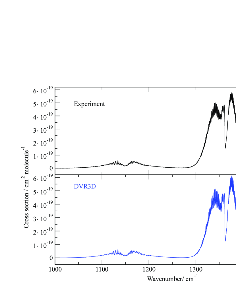
Figure 5: Comparison of absorption cross sections obtained at $T$ = 573.15 K for SO₂ experimentally (above) and from the hot line list (below).

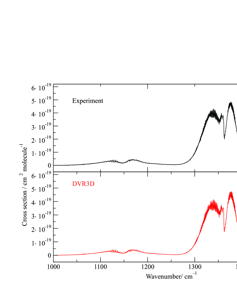
Figure 6: Comparison of absorption cross sections obtained at $T$ = 773.15 K for SO₂ via experimentally (above) and from the hot line list (below).

This spectral region considered contains both the $\nu_{1}$ and $\nu_{3}$ bands, and the intensity features are qualitatively well represented by the simulated cross sections. For 573.15 K (300 C) the integrated intensity across the 1000 $<\nu\ <$ 1500 cm^-1 spectral region is calculated as 3.43 $\times$ 10^-17 cm² molecule^-1, which is about 2% less than that for the experimental value, measured as 3.50 $\times$ 10^-17 cm² molecule^-1.

For 773.15 K (500 C) the integrated cross section across the same spectral region is calculated as 3.41 $\times$ 10^-17 cm² molecule^-1, which is roughly 6% less than that for the experimental value, 3.62 $\times$ 10^-17 cm² molecule^-1. This may be attributed to a small discrepancy observed in the P-branch of the $\nu_{3}$ band which is not obvious from Figure 6; the intensity here is slightly lower for the computed cross sections. Since this disagreement affects a specific region of the spectrum, it is unlikely wholly due to an error in the partition sum. The quality of the DMS may also be a contributing factor, in conjunction with the states involved in these transitions. Another source may be from the generation of the cross sections themselves; the line shape function used in constructing the theoretical cross sections is Gaussian, and therefore only considers thermal (Doppler) broadening, as opposed to a combination of thermal and pressure broadening (Voigt line shape). It is possible that neglecting the (unknown) pressure-broadening contribution in the line shape convolution is the source of this disagreement. Regardless of this discrepancy, use of a Voigt profile would considerably improve the overall quality of computed cross sections.

4.4 Cross Sections

Figures 7 - 10 display temperature-dependent calculated cross sections for the rotational and two fundamental bands of SO₂. All simulations are produced using the hot line list convolved with a Gaussian line shape function with HWHM = 0.5 cm^-1.

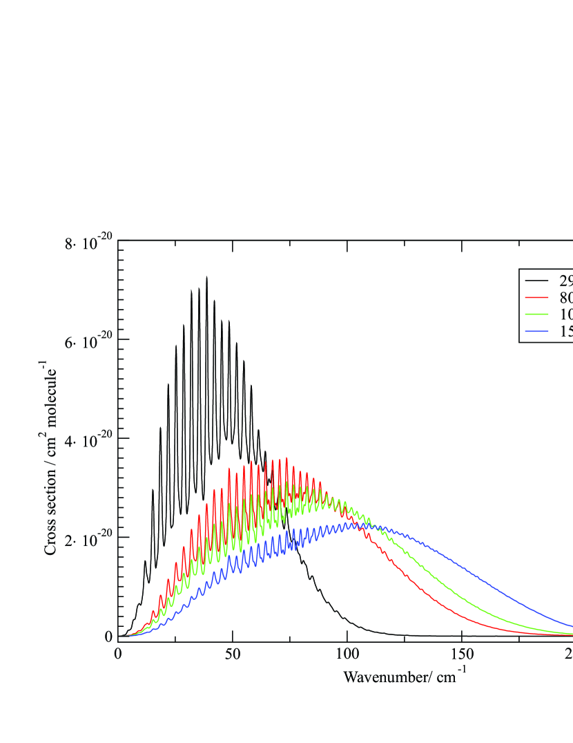
Figure 7: Temperature-dependent absorption cross sections for the rotational band of SO₂. The maximum peak heights decrease monotonically with temperature.

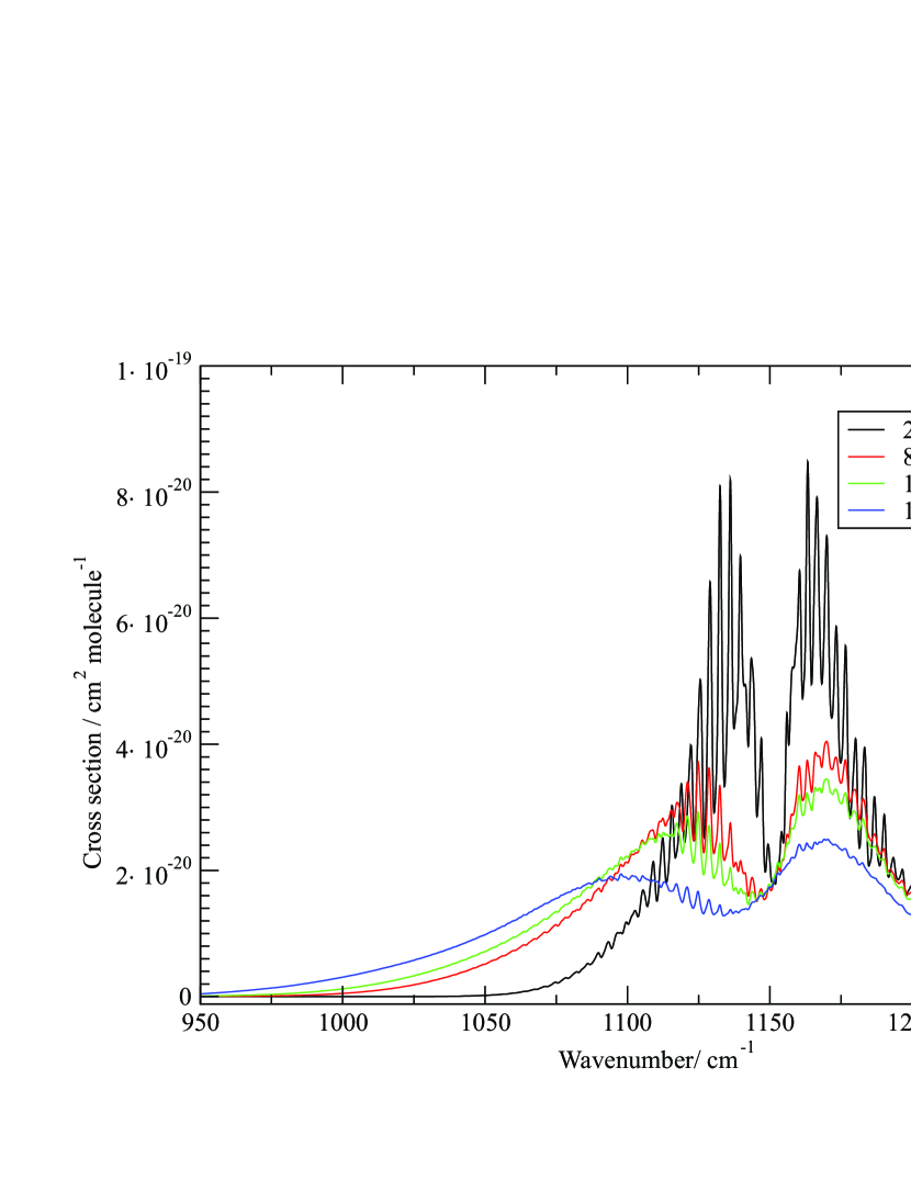
Figure 8: Temperature-dependent absorption cross sections for the $\nu_{1}$ band of SO₂. The contribution to the intensity beyond 1225 cm^-1 is due to the $\nu_{3}$ band. The maximum peak heights decrease monotonically with temperature.

Figure 9: Temperature-dependent absorption cross sections for the $\nu_{2}$ band of SO₂. The maximum peak heights decrease monotonically with temperature.

Figure 10: Temperature-dependent absorption cross sections for the $\nu_{3}$ band of SO₂. The maximum peak heights decrease monotonically with temperature.

Figure 11 shows an overview plot of the spectrum for 0 $<\nu\ <$ 8000 cm^-1($\lambda>1.25$ $\mu$m), highlighting the temperature-dependence of the cross section intensities. Again, this simulation is produced using the hot line list convolved with a Gaussian line shape function with HWHM = 2.0 cm^-1.

Figure 11: Temperature-dependent absorption cross sections for the entire $\lambda>1.25$ $\mu$m or 0 $<\nu\ <$ 8000 cm^-1 region of SO₂. The dips in the cross sections are progressively smoothed out with increading temperature.

5 Conclusion

A new hot line list for SO₂, called ExoAmes, has been computed containing 1.3 billion transitions. The line list is divided into an energy file and a transitions file. This is done using the standard ExoMol format (Tennyson et al., 2013) based on the method originally developed for the BT2 line list by Barber et al. (2006). The full line list can be downloaded from the CDS, via ftp://cdsarc.u-strasbg.fr/pub/cats/J/MNRAS/xxx/yy, or http://cdsarc.u-strasbg.fr/viz-bin/qcat?J/MNRAS//xxx/yy, as well as the exomol website, www.exomol.com. The line lists and partition function together with auxiliary data including the potential parameters and dipole moment functions, as well as the absorption spectrum given in cross section format (Hill et al., 2013), can all be obtained also from www.exomol.com as part of the extended ExoMol database (Tennyson et al., 2016).

SO₂ is one of three astrophysically-important sulphur oxides. A room temperature line list for SO₃ has already been computed (Underwood et al., 2013) and a hot line list has recently been completed. The results of these calculations will be compared with recent observations recorded at DTU. The comparison and the line list will be presented here soon.

Unlike SO₂ and SO₃, SO is an open shell system with a ${}^{3}\Sigma^{+}$ symmetry electronic ground states which therefore requires special treatment (Schwenke, 2015). A line list for this system will soon be computed with the program Duo (Yurchenko et al., 2016) which has been newly-developed for treating precisely this sort of problem.

References

- Adande et al. (2013) Adande G. R., Edwards J. L., Ziurys L. M., 2013, ApJ, 778
- Anderson et al. (1999) Anderson E., et al., 1999, LAPACK Users’ Guide, third edn. Society for Industrial and Applied Mathematics, Philadelphia, PA
- Arney et al. (2014) Arney G., Meadows V., Crisp D., Schmidt S. J., Bailey J., Robinson T., 2014, J. Geophys. Res., 119, 1860
- Azzam et al. (2016) Azzam A. A. A., Yurchenko S. N., Tennyson J., Naumenko O. V., 2016, MNRAS, p. (in preparation)
- Ballester et al. (1994) Ballester G. E., Mcgrath M. A., Strobel D. F., Zhu X., Feldman P. D., Moos H. W., 1994, Icarus, 111, 2
- Barber et al. (2006) Barber R. J., Tennyson J., Harris G. J., Tolchenov R. N., 2006, MNRAS, 368, 1087
- Barker (1979) Barker E. S., 1979, J. Geophys. Res., 6, 117
- Barton et al. (2015) Barton E. J., Yurchenko S. N., Tennyson J., Clausen S., Fateev A., 2015, J. Quant. Spectrosc. Radiat. Transf., 167, 126
- Belloche et al. (2013) Belloche A., Müller H. S. P., Menten K. M., Schilke P., Comito C., 2013, A&A, 559, A47
- Belyaev et al. (2008) Belyaev D., et al., 2008, J. Geophys. Res., 113
- Belyaev et al. (2012) Belyaev D. A., et al., 2012, Icarus, 217, 740
- Blackie et al. (2011) Blackie D., Blackwell-Whitehead R., Stark G., Pickering J. C., Smith P. L., Rufus J., Thorne A. P., 2011, J. Geophys. Res., 116, E03006
- Choi & Light (1992) Choi S. E., Light J. C., 1992, J. Chem. Phys., 97, 7031
- Chu et al. (1998) Chu P. M., Wetzel S. J., Lafferty W. J., Perrin A., Flaud J. M., Arcas P., Guelachvili G., 1998, J. Mol. Spectrosc., 189, 55
- Crockett et al. (2010) Crockett N. R., Bergin E. A., Wang S., Lis D. C., Bell T. A., et al. 2010, A&A, 521, L21
- Danielache et al. (2008) Danielache S. O., Eskebjerg C., Johnson M. S., Ueno Y., Yoshida N., 2008, J. Geophys. Res., 113, D17314
- Danielache et al. (2012) Danielache S. O., Hattori S., Johnson M. S., Ueno Y., Nanbu S., Yoshida N., 2012, J. Geophys. Res., 117, D24301
- Endo et al. (2015) Endo Y., Danielache S. O., Ueno Y., Hattori S., Johnson M. S., Yoshida N., Kjaergaard H. G., 2015, J. Geophys. Res., 120, 2546
- Flaud & Lafferty (1993) Flaud J.-M., Lafferty W. J., 1993, J. Mol. Spectrosc., 161, 396
- Franz et al. (2013) Franz H. B., Danielache S. O., Farquhar J., Wing B. A., 2013, Chem. Geology, 362, 56
- Freeman et al. (1984) Freeman D. E., Yoshino K., Esmond J. R., Parkinson W. H., 1984, Planet Space Sci., 32, 1125
- Greenberg & Hargis (1990) Greenberg K. E., Hargis P. J., 1990, J. Appl. Phys., 68, 505
- Grosch et al. (2015a) Grosch H., Fateev A., Clausen S., 2015a, J. Quant. Spectrosc. Radiat. Transf., 154, 28
- Grosch et al. (2015b) Grosch H., Fateev A., Clausen S., 2015b, J. Quant. Spectrosc. Radiat. Transf., 154, 28
- Grosch et al. (2015c) Grosch H., Sarossy Z., Fateev A., Clausen S., 2015c, J. Quant. Spectrosc. Radiat. Transf., 156, 17
- Grosch et al. (2013) Grosch H., Fateev A., Nielsen K. L., Clausen S., 2013, J. Quant. Spectrosc. Radiat. Transf., 130, 392
- Henningsen et al. (2008) Henningsen J., Barbe A., De Backer-Barilly M.-R., 2008, J. Quant. Spectrosc. Radiat. Transf., 109, 2491
- Hieta & Merimaa (2014) Hieta T., Merimaa M., 2014, Appl. Phys. B, 117, 847
- Hill et al. (2013) Hill C., Yurchenko S. N., Tennyson J., 2013, Icarus, 226, 1673
- Huang et al. (2008) Huang X., Schwenke D. W., Lee T. J., 2008, J. Chem. Phys., 129, 214304
- Huang et al. (2011a) Huang X., Schwenke D. W., Lee T. J., 2011a, J. Chem. Phys., 134, 044320
- Huang et al. (2011b) Huang X., Schwenke D. W., Lee T. J., 2011b, J. Chem. Phys., 134, 044321
- Huang et al. (2012) Huang X., Schwenke D. W., Tashkun S. A., Lee T. J., 2012, J. Chem. Phys., 136, 124311
- Huang et al. (2014) Huang X., Schwenke D. W., Lee T. J., 2014, J. Chem. Phys., 140, 114311
- Huang et al. (2015) Huang X., Schwenke D. W., Lee T. J., 2015, J. Mol. Spectrosc., 311, 19
- Huang et al. (2016) Huang X., Schwenke D. W., Lee T. J., 2016, J. Mol. Spectrosc.
- Kama et al. (2013) Kama M., López-Sepulcre A., Dominik C., Ceccarelli C., Fuente A., Caux E., et al. 2013, A&A, 556, A57
- Kaupi & Halonen (1992) Kaupi E., Halonen L., 1992, J. Chem. Phys., 96, 2933
- Khayat et al. (2015a) Khayat A. S., Villanueva G. L., Mumma M. J., Tokunaga A. T., 2015a, Icarus, 253, 130
- Khayat et al. (2015b) Khayat A. S., Villanueva G. L., Mumma M. J., Tokunaga A. T., 2015b, Icarus, 253, 130
- Klisch et al. (1997) Klisch E., Schilke P., Belov S. P., Winnewisser G., 1997, J. Mol. Spectrosc., 186, 314
- Kumar & Poirier (2015) Kumar P., Poirier B., 2015, Chem. Phys., 461, 34
- Kumar et al. (2015) Kumar P., Ellis J., Poirier B., 2015, Chem. Phys., 450-451, 59
- Lafferty et al. (1992) Lafferty W. J., et al., 1992, J. Mol. Spectrosc., 154, 51
- Lafferty et al. (1993) Lafferty W. J., Pine A. S., Flaud J.-M., Camy-Peyret C., 1993, J. Mol. Spectrosc., 157, 499
- Lafferty et al. (1996) Lafferty W. J., Pine A. S., Hilpert G., Sams R. L., Flaud J.-M., 1996, J. Mol. Spectrosc., 176, 280
- Leveque et al. (2015) Leveque C., Taieb R., Koeppel H., 2015, Chem. Phys., 460, 135
- Lodi & Tennyson (2010) Lodi L., Tennyson J., 2010, J. Phys. B: At. Mol. Opt. Phys., 43, 133001
- Lyons (2008) Lyons J. R., 2008, in Goodsite M. E., Johnson M. S., eds, Adv. Quantum Chem., Vol. 55, Applications of Theoretical Methods to Atmospheric Science. Academic Press, pp 57 – 74, doi:http://dx.doi.org/10.1016/S0065-3276(07)00205-5
- Martin et al. (2003) Martin S., Mauersberger R., Martin-Pintado J., Garcia-Burillo S., Henkel C., 2003, A&A, 411, L465
- Martin et al. (2005) Martin S., Martin-Pintado J., Mauersberger R., Henkel C., Garcia-Burillo S., 2005, ApJ, 620, 210
- Neale et al. (1996) Neale L., Miller S., Tennyson J., 1996, ApJ, 464, 516
- Nelson et al. (1980) Nelson R. M., Lane A. L., Matson D. L., Fanale F. P., Nash D. B., Johnson T. V., 1980, Science, 210, 784
- Partridge & Schwenke (1997) Partridge H., Schwenke D. W., 1997, J. Chem. Phys., 106, 4618
- Pearl et al. (1979) Pearl J., Hanel R., Kunde V., Maguire W., Fox K., Gupta S., Ponnamperuma C., Raulin F., 1979, Nature, 280, 755
- Ran et al. (2007) Ran H., Xie D., Guo H., 2007, Chem. Phys. Lett., 439, 280
- Rothman et al. (2013) Rothman L. S., et al., 2013, J. Quant. Spectrosc. Radiat. Transf., 130, 4
- Rufus et al. (2003) Rufus J., Stark G., Smith P. L., Pickering J. C., Thorne A. P., 2003, J. Geophys. Res., 108, 5011
- Rufus et al. (2009) Rufus J., Stark G., Thorne A. P., Pickering J. C., Blackwell-Whitehead R. J., Blackie D., Smith P. L., 2009, J. Geophys. Res., 114, E06003
- Schilke et al. (2001) Schilke P., Benford D. J., Hunter T. R., Lis D. C., Philips T. G., 2001, ApJS, 132, 281
- Schwenke (1996) Schwenke D. W., 1996, J. Phys. Chem., 100, 2867
- Schwenke (2015) Schwenke D. W., 2015, J. Chem. Phys., 142, 144107
- Sharpe et al. (2004) Sharpe S. W., Johnson T. J., Sams R. L., Chu P. M., Rhoderick G. C., Johnson P. A., 2004, Appl. Spectrosc., 58, 1452
- Shirin et al. (2003) Shirin S. V., Polyansky O. L., Zobov N. F., Barletta P., Tennyson J., 2003, J. Chem. Phys., 118, 2124
- Stark et al. (1999) Stark G., Smith P. L., Rufus J., Thorne A. P., Pickering J. C., Cox G., 1999, J. Geophys. Res., 104, 6585
- Stoiber & Jepsen (1973) Stoiber R. E., Jepsen A., 1973, Science, 182, 577
- Sutcliffe et al. (1988) Sutcliffe B. T., Miller S., Tennyson J., 1988, Comput. Phys. Commun., 51, 73
- Tennyson & Sutcliffe (1982) Tennyson J., Sutcliffe B. T., 1982, J. Chem. Phys., 77, 4061
- Tennyson & Sutcliffe (1992) Tennyson J., Sutcliffe B. T., 1992, Intern. J. Quantum Chem., 42, 941
- Tennyson & Yurchenko (2012) Tennyson J., Yurchenko S. N., 2012, MNRAS, 425, 21
- Tennyson et al. (2004) Tennyson J., Kostin M. A., Barletta P., Harris G. J., Polyansky O. L., Ramanlal J., Zobov N. F., 2004, Comput. Phys. Commun., 163, 85
- Tennyson et al. (2013) Tennyson J., Hill C., Yurchenko S. N., 2013, in 6th international conference on atomic and molecular data and their applications ICAMDATA-2012. AIP, New York, pp 186–195, doi:10.1063/1.4815853
- Tennyson et al. (2016) Tennyson J., Yurchenko S. N., The ExoMol team 2016, J. Mol. Spectrosc.
- Tinetti et al. (2013) Tinetti G., Encrenaz T., Coustenis A., 2013, A&A Rev, 21, 1
- Ulenikov et al. (2009) Ulenikov O. N., Bekhtereva E. S., Horneman V.-M., Alanko S., Gromova O. V., 2009, J. Mol. Spectrosc., 255, 111
- Ulenikov et al. (2010) Ulenikov O. N., Bekhtereva E. S., Gromova O. V., Alanko S., Horneman V.-M., Leroy C., 2010, Mol. Phys., 108, 1253
- Ulenikov et al. (2011) Ulenikov O. N., Gromova O. V., Bekhtereva E. S., Bolotova I. B., Leroy C., Horneman V.-M., Alanko S., 2011, J. Quant. Spectrosc. Radiat. Transf., 112, 486
- Ulenikov et al. (2012) Ulenikov O. N., Gromova O. V., Bekhtereva E. S., Bolotova I. B., Konov I. A., Horneman V.-M., Leroy C., 2012, J. Quant. Spectrosc. Radiat. Transf., 113, 500
- Ulenikov et al. (2013) Ulenikov O. N., Onopenko G. A., Gromova O. V., Bekhtereva E. S., Horneman V.-M., 2013, J. Quant. Spectrosc. Radiat. Transf., 130, 220
- Underwood (2016) Underwood D. S., 2016, PhD thesis, University College London
- Underwood et al. (2013) Underwood D. S., Tennyson J., Yurchenko S. N., 2013, Phys. Chem. Chem. Phys., 15, 10118
- Visscher et al. (2006) Visscher C., Lodders K., Fegley Jr. B., 2006, ApJ, 648, 1181
- Voitsekhovskaya et al. (2013) Voitsekhovskaya O. K., Kashirskii D. E., Egorov O. V., 2013, Russian Phys. J., 56, 473
- Whitehill et al. (2013) Whitehill A. R., Xie C., Hu X., Xie D., Guo H., Ono S., 2013, Proc. Nat. Acad. Sci., 110, 17697
- Xie et al. (2000) Xie D. Q., Guo H., Bludsky O., Nachtigall P., 2000, Chem. Phys. Lett., 329, 503
- Yamamura et al. (1999) Yamamura I., de Jong T., Osaka T., Cami J., Waters L. B. F. M., 1999, A&A, 341, L9
- Yurchenko et al. (2016) Yurchenko S. N., Lodi L., Tennyson J., Stolyarov A. V., 2016, Comput. Phys. Commun.
- Ziurys (2006) Ziurys L. M., 2006, Proc. Nat. Acad. Sci., 103, 12274
- van der Tak et al. (2003) van der Tak F. F. S., Boonman A. M. S., Braakman R., van Dishoeck E. F., 2003, A&A, 412, 133