New orbital ephemerides for the dipping source 4U 1323-619: constraining the distance to the source

Abstract

Context. 4U 1323-619 is a low mass X-ray binary system that shows type I X-ray bursts and dips. The most accurate estimation of the orbital period is 2.941923(36) hrs and a distance from the source that is lower than 11 kpc has been proposed.

Aims. We aim to obtain the orbital ephemeris, the orbital period of the system, as well as its derivative to compare the observed luminosity with that predicted by the theory of secular evolution.

Methods. We took the advantage of about 26 years of X-ray data and grouped the selected observations when close in time. We folded the light curves and used the timing technique, obtaining 12 dip arrival times. We fit the delays of the dip arrival times both with a linear and a quadratic function.

Results. We locate 4U 1323-619 within a circular area centred at RA (J2000)= 201.6543^∘ and DEC (J2000)= -62.1358^∘ with an associated error of 0.0002^∘, and confirm the detection of the IR counterpart already discussed in literature. We estimate an orbital period of P=2.9419156(6) hrs compatible with the estimations that are present in the literature, but with an accuracy ten times higher. We also obtain a constraint on the orbital period derivative for the first time, estimating $\dot{P}=(8\pm 13)\times 10^{-12}$ s/s. Assuming that the companion star is in thermal equilibrium in the lower main sequence, and is a neutron star of 1.4 M_⊙, we infer a mass of 0.28$\pm$0.03 M_⊙ for the companion star. Assuming a distance of 10 kpc, we obtained a luminosity of (4.3$\pm$0.5)$\times 10^{36}$ erg s^-1, which is not in agreement with what is predicted by the theory of secular evolution. Using a 3D extinction map of the K_s radiation in our Galaxy, we obtain a distance of 4.2${}^{+0.8}_{-0.7}$ kpc at 68% confidence level. This distance implies a luminosity estimation of (0.8$\pm$0.3)$\times 10^{36}$ erg s^-1, which is consistent with the adopted scenario in which the companion star is in thermal equilibrium.

1 Introduction

Table 1: Observation log.

Point	Satellite/Instrument	Observation ID	Start time	Stop time	Tfold
			(UT)	(UT)	(TJD;TDB)
1	EXOSAT/ME	1401	1985 Feb 11 18:48:49	1985 Feb 13 04:39:18	6108.48892929229
2	ASCA/GIS2	42005000	1994 Aug 04 12:21:11	1994 Aug 04 20:10:47	9568.66237498892
3	RXTE/PCA	P20066-02-01-00, P20066-02-01-01, P20066-02-01-02,	1997 Apr 25 22:04:48	1997 Apr 28 03:44:49	10565.04185436878
		P20066-02-01-03, P20066-02-01-04
4	BeppoSAX/MECS	20102001	1997 Aug 22 17:06:09	1997 Aug 24 02:02:39	10683.398658095225
5	RXTE/PCA	P40040-01-01-000, P40040-01-01-00, P40040-01-02-000,	1999 Jan 18 02:42:30	1999 Mar 13 09:10:46	11223.245347406
		P40040-01-02-00, P40040-01-03-000, P40040-01-03-00
6	ASCA/GIS2	47015000	2000 Feb 02 12:16:04	2000 Feb 04 23:19:15	11577.746691772565
7	XMM/Epic-pn	0036140201	2003 Jan 29 09:03:42	2003 Jan 29 22:57:07	12668.666973091815
8	RXTE/PCA	P70050-03-01-00, P70050-03-01-01, P70050-03-01-02	2003 Sep 25 07:54:56	2003 Sep 25 23:57:20	12907.661355385295
9	RXTE/PCA	P90062-03-01-010, P90062-03-01-01, P90062-03-01-00,	2004 Dec 30 21:46:40	2004 Dec 31 13:53:03	13370.240516395665
		P90062-03-01-02
10	Suzaku/XIS0	401002010	2007 Jan 09 11:50:53	2007 Jan 10 21:58:37	14110.204689820065
11	RXTE/PCA	P95442-01-01-00, P95442-01-01-01, P95442-01-01-02,	2010 Dec 25 08:01:54	2011 Mar 28 12:14:06	15601.92228420802
		P96405-01-01-01, P96405-01-02-00, P96405-01-02-01
		P96405-01-01-00,
12	Chandra/HETG	13721, 14377	2011 Dec 19 01:03:11	2011 Dec 24 19:01:07	15916.91815760006

4U 1323-619 is a low mass X-rays binary system (LMXB) that was discovered by Forman et al. (1978) and identified as persistent by Warwick et al. (1981). Periodic dips and type I bursts were discovered in the European X-ray Observatory Satellite (EXOSAT) light curves (van der Klis et al. 1985; Parmar et al. 1989). The matter transferred from the companion star, impacting onto the outer accretion disc, forms a bulge of cold (and/or partially ionised) matter that photoelectrically absorbs part of the X-ray emission, which comes from the inner region of the system. The shape of a dip is generally irregular and varies from one cycle to another. However, the periodic occurrence of the dips in the light curve is strictly connected to the orbital motion of the binary system and the study of their periodicity can give information on the orbital period of the system. From EXOSAT and BeppoSAX lightcurves, Parmar et al. (1989) and Bałucińska-Church et al. (1999) inferred an orbital period of 2.932(5) hrs and 2.94(2) hrs, respectively. Levine et al. (2011), studying the RossiXTE/ASM 1.5-12 keV light curve from 1996 to 2011, find an orbital period of 2.941923(36) hrs. Although the light curves of 4U 1323-619 show dips, they do not show eclipses, which implies that the source has an inclination angle $i$ between 60^∘ and 80^∘ (Frank et al. 1987). Zolotukhin et al. (2010), using a Chandra observation performed in continuous clocking mode, obtain the X-ray position of the source that, however, suffers from the indetermination in one direction because of the Chandra observational mode. The same authors also estimate the X-ray position of the source with an associated error of 3” using data of the X-ray Multi Mirror (XMM-Newton) mission. Zolotukhin et al. (2010), analysing the 2MASS catalogue, identify two possible infrared counterparts of 4U 1323-619 that are associated with the X-ray position estimated using XMM-Newton data. From the intersection of the positional error boxes of Chandra and XMM-Newton, they suggest that the probable infrared counterpart is a source with a magnitude of 18.12$\pm$0.20 in the K_s band.

The spectral analysis of the source shows that the equivalent column density of neutral hydrogen, N_H, is large and depends on the model used to fit the spectra and on the energy band covered. Bałucińska-Church et al. (2009) find N${}_{H}=(3.2^{+0.1}_{-0.1})\times 10^{22}$ cm^-2 using Suzaku data, Boirin et al. (2005) infer N${}_{H}=(3.5^{+0.1}_{-0.2})\times 10^{22}$ cm^-2 using XMM-Newton data and Parmar et al. (1989) obtained N${}_{H}=(4.0\pm 0.3)\times 10^{22}$ cm^-2 using EXOSAT data. Smale (1995) suggested that the large extinction to the source also explains why the optical counterpart has not been detected yet. Furthermore, Bałucińska-Church et al. (1999) suggested the possible presence of a local dust halo surrounding 4U 1323-619. The main effect of the halo is to absorb part of the source radiation owing to its optical depth, which depends on the inverse of the incoming radiation energy (Predehl & Schmitt 1995).

The spectral analysis of 4U 1323-619 also highlights that the energy spectrum is dominated by a power-law component. Parmar et al. (1989) found a photon index $\Gamma$ of the power-law component of 1.53$\pm$0.07, Boirin et al. (2005) obtain a $\Gamma$ of $1.9^{+0.06}_{-0.10}$ and, adopting a cut-off power-law component, Bałucińska-Church et al. (2009) find a $\Gamma$ of $1.67^{+0.10}_{-0.03}$ and an energy cut-off of 85${}^{+77}_{-35}$ keV. Galloway et al. (2008), analysing the type I X-ray bursts properties of 4U 1323-619 with data obtained with the proportional counter array (PCA) on board the RXTE mission, only infer an upper limit for the distance from the source because they do not find any evidence of photospheric radius expansion (PRE). The upper limit is of 11 kpc, assuming a companion star with cosmic abundances, and of 15 kpc, assuming a pure hydrogen companion star. Furthermore, the same authors show that the light curves demonstrate many double bursts where the secondary bursts are fainter and suggest that this can be explained taking into account a mixed composition of hydrogen and helium of the companion star, which causes short recurrence bursts generated by the hydrogen ignition onto the neutron star. In addition, using EXOSAT/ME data in the energy band 1.5-11 keV, Parmar et al. (1989) gave a lower limit of 10 kpc for the distance from the source on the basis of the observed properties of the bursts.

Zolotukhin et al. (2010), studying the photometric properties of 4U 1323-619 in the IR band and assuming a distance of 10 kpc, find a discrepancy of one order of magnitude between the observed value of the flux and that predicted by a model that describes the system as an accretion disk illuminated by a central spherical hot corona, which has a luminosity of 5.2$\times 10^{36}$ erg s^-1 in the 0.1-10 keV band (Boirin et al. 2005). Based on this discrepancy, they suggest a distance from the source between 4 and 5 kpc.

In this work, we find the first orbital linear and quadratic ephemerides of 4U 1323-619, using all the available X-ray pointing observations from 1985 to 2011. We find a weak constraint on the orbital period derivative. We compare the obtained results with the prediction of the secular evolution of the binary system (see e.g. King 1988; Verbunt 1993) and suggest that the source distance is less than 5 kpc (close to 4.2 kpc for a companion star in thermal equilibrium).

2 Observation and data reduction

Table 2: Best-fit parameters obtained by fitting the dips in the folded light curves.

Point	Phase interval	Y1	Y2	Y3	$\phi_{1}$	$\phi_{2}$	$\phi_{3}$	$\phi_{4}$	$\chi^{2}_{red}$ (d.o.f.)
		count s-1	count s-1	count s-1
1	0 - 1	4.88$\pm$ 0.04	3.29$\pm$ 0.05	4.94$\pm$ 0.04	0.248$\pm$ 0.008	0.322$\pm$ 0.008	0.519$\pm$ 0.007	0.604$\pm$ 0.008	1.18(506)
2	0 - 1	1.41$\pm$0.02	0.78$\pm$0.02	1.51$\pm$0.02	0.351$\pm$0.006	0.384$\pm$0.005	0.598$\pm$0.005	0.621$\pm$0.006	1.66(438)
3	0.6 - 1.6	19.85$\pm$0.05	15.62$\pm$0.07	20.32$\pm$0.06	0.920$\pm$0.005	1.009$\pm$0.004	1.159$\pm$0.005	1.301$\pm$0.005	5.44(482)
4	0 - 1	0.954$\pm$0.008	0.634$\pm$0.008	0.961$\pm$0.010	0.359$\pm$0.007	0.432$\pm$0.006	0.643$\pm$0.008	0.744$\pm$0.009	1.56(506)
5	0 - 1	21.21$\pm$0.05	16.53$\pm$0.06	21.06$\pm$0.05	0.334$\pm$0.004	0.414$\pm$0.004	0.580$\pm$0.003	0.651$\pm$0.003	4.89(506)
6	0 - 1	1.231$\pm$0.012	0.724$\pm$0.011	1.260$\pm$0.012	0.294$\pm$0.008	0.409$\pm$0.007	0.615$\pm$0.007	0.676$\pm$0.007	1.50(506)
7	0.3 - 1.3	28.4$\pm$0.2	22 (fixed)	27.4$\pm$0.2	0.632$\pm$0.008	0.699$\pm$0.007	0.937$\pm$0.007	0.983$\pm$0.007	15.65(506)
8	0.6 - 1.6	19.31 $\pm$0.08	14.5 (fixed)	18.96$\pm$0.07	0.936$\pm$0.006	1.052$\pm$0.005	1.132$\pm$0.006	1.246$\pm$0.007	2.72(495)
9	0.9 - 1.9	17.34$\pm$0.13	12.83$\pm$0.10	17.62$\pm$0.12	1.224$\pm$0.007	1.259$\pm$0.008	1.531$\pm$0.006	1.589$\pm$0.006	4.94(495)
10	0.3 - 1.3	0.922$\pm$0.009	0.500$\pm$0.009	0.932$\pm$0.010	0.629$\pm$0.006	0.686$\pm$0.005	0.881$\pm$0.008	1.028$\pm$0.009	1.65(505)
11	1 - 2	18.42$\pm$0.11	13.64$\pm$0.11	18.39$\pm$0.09	1.278$\pm$0.006	1.338$\pm$0.006	1.537$\pm$0.008	1.630$\pm$0.010	2.09(505)
12	0.27 - 1.27	0.781$\pm$0.007	0.494$\pm$0.005	0.813$\pm$0.007	0.561$\pm$0.006	0.607$\pm$0.005	0.914$\pm$0.004	0.956$\pm$0.005	2.72(505)

To analyse the dips arrival times of 4U 1323-619, we used all the available X-ray archival data that include RXTE, Chandra, XMM-Newton, Suzaku, BeppoSAX, EXOSAT and ASCA observations.

We used the Chandra data of the ObsIDs 13721, 14377, and 3826. Both the ObsID 13721 and ObsID 14377 data were collected in December 2011 in timed graded mode, while the data of the ObsID 3826 were taken in continuous clocking mode in September 2003. To process the Chandra data we used CIAO v. 4.7. The observations have been reprocessed with the chandra_repro routine. We used the ObsID 13721 to obtain an accurate estimation of the X-ray source position using the Chandra tool tg_findzo. The revised coordinates for 4U 1323-619 are: RA (J2000)= 201.6543^∘ and DEC (J2000)= -62.1358^∘, with an associated error of 0.6”, which represents the 90% confidence level Chandra positional accuracy.
We report the Chandra/HETG image of 4U 1323-619 that was obtained from the reprocessed level 2 data in Fig. 1. The green and black circles indicate the X-ray source position shown in this work and in Zolotukhin et al. (2010), respectively. The infrared sources, A and B, suggested by Zolotukhin et al. (2010) are indicated with crosses and have an error circle with a radius of 0.2”. The B source is located inside a circular area, which has a radius of 0.2” that has been determined with the 2MASS catalogue. On the basis of our results we confirm that the source B is the infrared counterpart of 4U 1323-619 as suggested by Zolotukhin et al. (2010). Hereafter we use the new X-ray Chandra coordinates to apply the barycentric corrections.
We applied the barycentric corrections to the Level 2 events file using the axbary tool and extracted the first diffraction orders and background-subtracted HEG + MEG light curves using the dmextract tool. To subtract the background from the light curves, we selected a background events extraction region of 5” of radius, far away from the real source position.

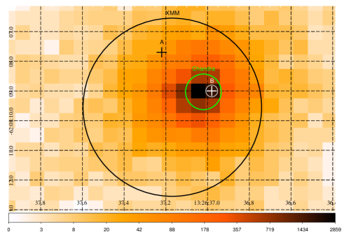
Figure 1: Chandra/HETG image of 4U 1323-619. The colour scale reports the number of photons. The green circle indicates the X-ray position obtained in this work, while the black circle indicates the position obtained by Zolotukhin et al. (2010) using XMM-Newton data. The A and B crosses are the two candidate infrared counterparts identified by Zolotukhin et al. (2010).

(a)

(b)

Figure 2: 1st order background subtracted Chandra/HETG light curves of the observations 14377 (a) and 13721 (b) in the energy range 0.5-10 keV. The light curve (a) starts on 19 December 2011 at 01:03:10 UT, while the light curve (b) starts on 23 December 2011 at 20:11:09 UT. The bin time is of 24 s.

The available RXTE/PCA observations span a period of about 13 years (from 1997 to 2011). We produced background-subtracted light curves, including all the energy channels and obtained the data from the HEASARC data archive. These light curves have a temporal resolution of 0.125 s and the barycentric corrections have been applied using the faxbary tool.
The only available observation of XMM-Newton/Epic-pn is the ObsID 0036140201 of January 2003, performed in timing mode. The data have been processed with the epproc tool of the Scientific Analysis System (SAS) v. 14.0.0 and the barycentric corrections have been applied with the barycen tool. The extraction region of the source photons has been chosen on the basis of the analysis of the histogram showing the number of photons versus the RAWX coordinate of the image. We selected a box region with a width of 21 RAWX and centred at the RAWX coordinate of the peak of the photons’ distribution (RAWX=36). Thus, we extracted the light curve with the evselect routine, selecting events with PATTERN$\leq$4 (single and double pixel events) and FLAG=0 (to ignore spurious events), in the energy range between 0.5 and 10 keV. We binned the resulting light curve at 1 s.
The available Suzaku observation of 4U 1323-619 is the ObsID 401002010 of January 2007. This has been processed with the aepipeline routine and the two available data formats (3X3 and 5X5) have been unified with each other. We applied the barycentric corrections to the events file with the aebarycen routine. We extracted the 0.2-10 keV light curve using the xselect tool and adopting a circular region around the brightest pixel of the source with a radius of 50”. We used a bin time of 16 s.
We also used the EXOSAT/ME observation performed on February 1985. The light curve has been extracted in the energy range between 1 and 8 keV with a bin time of 10 s and the barycentric corrections have been applied with the ftool earth2sun.
Furthermore, we used two ASCA/GIS2 observations: the first has been taken on August 1994 and the second one on February 2000. Both observations were performed in medium bit rate mode and the light curves were extracted with a bin time of 0.5 s. We applied the barycentric corrections using the timeconv ftool.
Finally, the only available observation of BeppoSAX is of August 1997. The BeppoSAX/MECS light curve has been extracted with the xselect ftool in a circular region of 4’ of radius, without energy filters and with a bin time of 4 s. The barycentric corrections have been applied with the ftool earth2sun.

3 Data analysis

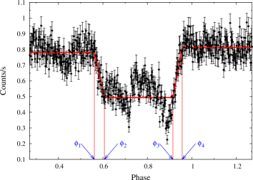
Figure 3: Folded light curve of the jointed Chandra observations ObsID 14377 and ObsID 13721. The red line is the step-and-ramp function that better fits the dip. The blue arrows highlight the phases of ingress ($\phi_{1}$ and $\phi_{2}$) and egress ($\phi_{3}$ and $\phi_{4}$) of the dip.

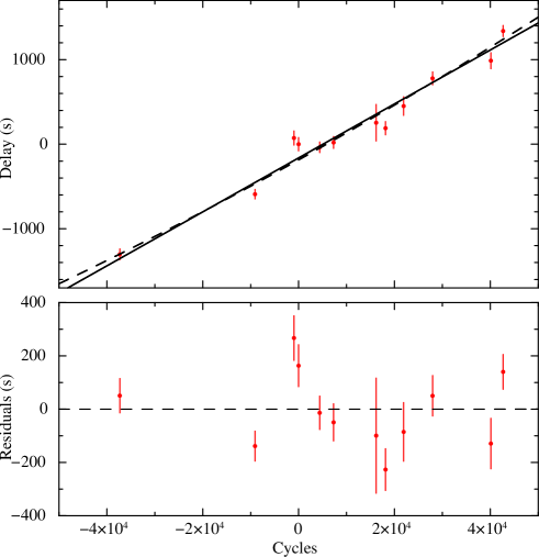
Figure 4: Upper panel: delays of the dip arrival times (calculated with respect to P₀ of 10590.864 s and T₀ of 10683.3987 TJD) as a function of the number of cycles. Both the linear and the quadratic models are shown as a solid and a dashed line, respectively. Lower panel: residuals associated with respect to the linear fit.

Figure 5: Folded RXTE/ASM light curves of 4U 1323-619 in the 2-10 keV energy band using the T₀ and orbital period suggested by Levine et al. (2011) (left panel) and the linear ephemeris shown in Eq. 2 (right panel). We adopted 14 phase-bins per period.

The whole analysed data-set spans a temporal range of about 26 years. All the selected observations have been grouped when close in time to obtain folded light curves to increase the statistics of the dips. We grouped the Chandra ObsIDs 13721 and 14377. The light curves of these observations are separately shown in Fig. 2a and 2b with a bin time of 24 s. The curves have been extracted from the first diffraction order of the HETG grating and the individual observations have a duration of about 62 and 80 ks, respectively. In the ObsID 14377 five dips occur, plus one more at the beginning of the observation that is only partially visible. In addition, during the observation 13 721 seven dips occur, plus one more that is partially visible at the beginning of the observation. In both observations several Type I bursts occur. The persistent emission is mainly at about 0.8 counts/s and the count-rate at the bottom of the dips is close to 0.3 counts/s.
Three RXTE/PCA observations have been ruled out from our analysis: the observation whose ObsID is P40040-01-02-01 because the dip is only partially visible in the light curve, as well as the observations whose ObsIDs are P96405-01-03-00 and P96405-01-04-00, owing to the lack of dips. We furthermore excluded four additional RXTE/PCA observations from our analysis (ObsIDs P96405-01-05-00, P96405- 01-05-01, P96405-01-05-02, and P96405-01-05-03) and one Chandra observation (ObsID 3826) owing to the fact that their folded light curves show a high count-rate variability outside the dips that does not allow us to obtain a valid fit for the dips by using the step-and-ramp function that we define below.
After this preventive selection process, we analysed 12 grouped and barycentric-corrected light curves that contain a total of 95 dips. The observations that we selected for the analysis, as well as their grouping, are shown in Tab. 1. Bursts were excluded from each light curve by removing the segments starting 5 s before the rise time of each burst and ending 100 s after the peak time. We verified that the shape of the dips in each light curve is quite similar from one cycle to another and folded the light curves with a reference time and a trial period (T_fold and P₀, respectively). To estimate the dip arrival time, we adopted the same procedure used by Iaria et al. (2015). For each light curve T_fold is defined as the average value between the start and stop time of the observation. We fit the dip in each folded light curve with a step-and-ramp function that involves seven parameters: the count-rate before (Y₁), during (Y₂) and after (Y₃) the dip, and the phases of ingress ($\phi_{1}$ and $\phi_{2}$) and egress ($\phi_{3}$ and $\phi_{4}$) of the dip. We show the step-and-ramp function fitting the folded light curve of the joint Chandra observations ObsID 14377 and ObsID 13721 in Fig. 3.
The phase of the dip arrival has been estimated as $\phi_{dip}=(\phi_{1}+\phi_{4})/2$. The corresponding dip arrival time is given by $T_{dip}=T_{fold}+\phi_{dip}P_{0}$.
The values of the $\chi^{2}_{red}$ in Tab. 2 are quite high. We can assume that this is a direct cause of the underestimation of the errors associated with the fitted data points. The uncertainties of all these data points can be increased by a constant factor to have a $\chi^{2}_{red}$ equal to 1, multiplying the uncertainties on the fitting parameters by a factor equal to the $\sqrt{\chi^{2}_{red}}$ of the fit. As a consequence of this, for the calculations of the uncertainty on the fitting parameters, all the uncertainties relative to the values of $\phi_{dip}$ have been rescaled by the factor $\sqrt{\chi^{2}_{red}}$, when the best-fit model gave a $\sqrt{\chi^{2}_{red}}$ greater than 1. Moreover, we use a trial orbital period P₀ of 10590.864 s and a reference epoch T₀ of 10683.4663 TJD to obtain the delays of the dips’ arrival times with respect to the reference epoch T₀. We choose the values of P₀ and T₀ arbitrarily, which are similar to those given by Levine et al. (2011). The values of T_fold are shown in Table 1, the best-fit parameters and the $\chi^{2}_{red}$ obtained by fitting the dips are shown in Table 2. Finally, the dip arrival times, the cycle and the delays for each observation are shown in Table 3.
First, we fit the obtained delays as a function of cycles with a linear function, taking into account only the errors associated with the delays. The fitting function is

$$y(N)=a+bN,$$ (1)

where N is the cycle number, $b$ is the correction to the trial orbital period ($\Delta P_{0}$) in seconds, and $a$ is the correction to the trial reference epoch ($\Delta T_{0}$) in seconds. Thus, we obtain a first estimation of the corrections to the reference epoch and to the orbital period. Taking into account the error associated with the number of the cycles ($\Delta x$), we obtain a total error $\Delta_{tot}=\sqrt{(\Delta y)^{2}+(b*\Delta x)^{2}}$, where $\Delta y$ is the error associated with the dip arrival time (see Iaria et al. 2014). We repeated the fitting procedure, obtaining a $\chi^{2}(d.o.f.)$ of 37.81(10). For the same reason adduced before, the uncertainties of the parameters returned by the linear fit have been rescaled by the factor $\sqrt{\chi^{2}_{red}}$, when the best-fit model gave a $\sqrt{\chi^{2}_{red}}$ greater than 1. The best-fit model parameters are shown in Table 4. The orbital ephemeris obtained with the linear model is

$$T_{dip}(N)={\rm TJD(TDB)}\;10683.4644(5)+\frac{10590.896(2)}{86400}N,$$ (2)

where 10683.4644(5) TJD and 10590.896(2) s are the reference epoch and orbital period, respectively. The associated errors are at 68% confidence level.
We also try to fit the delays using a quadratic function:

$$y(N)=a+bN+cN^{2},$$ (3)

where $a$ is the reference epoch correction ($\Delta T_{0}$) in seconds, $b$ is the orbital period correction ($\Delta P_{0}$) in seconds, and $c=\frac{1}{2}P_{0}\dot{P}$ in units of seconds. The best-fit model parameters are reported in Table 2. The fit returns a value of the $\chi^{2}(d.o.f.)$ of 36.04(9), while the F-test probability of chance improvement with respect to the previous linear fit is only of 52%. This suggests that, adopting the quadratic ephemeris, we do not improve the fit significantly. The orbital ephemeris obtained with the quadratic fit is

$$\begin{split}T_{dip}(N)={\rm TJD(TDB)}\;10683.4641(7)+\frac{10590.896(2)}{86400}N+\\ +\frac{4(7)\times 10^{-8}}{86400}N^{2},\end{split}$$ (4)

where 10683.4641(7) TJD is the new reference epoch, 10590.896(2) s is the new orbital period and $\dot{P}=(0.8\pm 1.3)\times 10^{-11}s/s$ is the orbital period derivative obtained by the $c$ parameter that was returned by the fit. The associated errors are at 68% confidence level. In the upper panel of Fig. 4 we show the delays versus the orbital cycles and, superimposed, two best-fit models, i.e. the linear and the quadratic ephemeris. At the bottom, the residuals resulting from the linear fit are shown. The maximum discrepancy between the delays and the linear best-fit model is of about 300 s, which is about 2.8% of the orbital period.

Table 3: Journal of arrival times of the X-ray dips obtained from each folded light curve. The number of dips in each grouped observation is also shown.

Point	Dip time	Cycle	Delay	Number of
	(TJD;TDB)		(s)	dips
1	6108.5412(7)	-37322	-1303$\pm$64	12
2	9568.7220(7)	-9094	-592$\pm$56	2
3	10565.0554(10)	-966	73$\pm$84	8
4	10683.4663(9)	0	0 $\pm$79	11
5	11223.3058(7)	4404	-36$\pm$63	9
6	11577.8062(8)	7296	20$\pm$70	7
7	12668.766(3)	16196	254$\pm$216	5
8	12907.6725(9)	18145	189$\pm$78	4
9	13370.2904(13)	21919	451$\pm$110	6
10	14110.3063(9)	27956	779$\pm$76	10
11	15601.9779(11)	40125	988$\pm$95	7
12	15917.0112(8)	42695	1339$\pm$65	14

Table 4: Best-fit values obtained from the linear and quadratic fits on the delays of the dips arrival times.

Parameter	Linear	Quadratic
a (s)	-163 $\pm$ 23	-186 $\pm$ 29
b ($\times 10^{-3}$ s)	31.9 $\pm$ 0.9	32 $\pm$ 1
c ($\times 10^{-8}$ s)	-	4 $\pm$ 7
$\chi^{2}$(d.o.f)	37.81(10)	36.04(9)

To verify the goodness of the linear ephemeris shown in Eq. 2, we folded the RXTE/ASM light curve in the 2-10 keV energy band. This light curve covers a time interval of 15.5 years (from 5 January 1996 to 24 September 2011) and barycentric corrections have been applied using the faxbary tool. We show the folded light curve using the reference epoch and orbital period suggested by Levine et al. (2011) and by our linear ephemeris in the left and right panels of Fig. 5, respectively. We adopted 14 phase bins per period (each phase bin corresponds to $\sim$757 s). We note that, using T₀ and P_orb from Eq. 2, the dip occurs at phase zero, while using the values from Levine et al. (2011), the dip occurs at a phase close to 0.1.

4 Spectral analysis

We present the spectral analysis of 4U 1323-619 performed with INTEGRAL data. This analysis is useful in Sect. 5 when extracting the unabsorbed flux of the source between 0.5 and 100 keV, to obtain an estimation of the luminosity.
We found a number of INTEGRAL pointings (science windows, SCW) collected on 2003 July 10–13 in the field of 4U 1323-619. To maximize the spectral response, we selected only SCWs (with a typical duration of 3 ks) with the source located within 4.5^∘ and 3.5^∘ from the centre of the IBIS and JEM-X FOVs, respectively. Thus, we analysed IBIS/ISGRI (Lebrun et al. 2003) data of 80 SCWs and JEM-X2 (Lund et al. 2003) data of 51 SCWs (JEM-1 was switched-off at that time) with the standard INTEGRAL software OSA 10.1 (Courvoisier et al. 2003) We verified that, in the JEM-X2 lightcurve, no type-I bursts were present and that the source flux was almost constant, so that, an averaged spectra (3-35 keV) has been extracted in 16 channels for a total exposure time of 156 ks. Because of the faintness of the source in hard X-rays, the ISGRI spectrum has been extracted by the total (about 198 ks) mosaic image with the mosaic_spec tool in four energy bins, spanning from 22 keV up to 65 keV.

The spectral analysis was performed using XSPEC v. 12.8.2 (Arnaud 1996). We modelled the joint JEM-X2 and ISGRI spectrum with a thermal Comptonisation (nthComp in XSPEC). This spectral component takes into account the nature of the seed photons (represented by the $inp\_type$ parameter that is equal to 0 for blackbody seed photons or to 1 for disk blackbody seed photons), the temperature kT_bb of the seed photons, the electron temperature kT_e, an asymptotic power-law photon index $\Gamma$, the redshift, as well as a normalisation constant. The absorption that is due to the interstellar medium has been taken into account by using the TBabs model with the chemical abundances of Asplund et al. (2009) and the cross-sections of Verner et al. (1996). The energy domain of the spectrum, however, does not enable us to well constrain the value of N_H. As a consequence of this, we fix the column density of neutral hydrogen to the value found by Parmar et al. (1989), which is also the highest available in literature. The fit gives a $\chi_{red}^{2}$ of 1.07 with 11 degrees of freedom. The best-fit parameters are shown in Tab. 5, while the deconvolved model and the resulting residuals in unity of $\sigma$ are shown in Fig. 6.

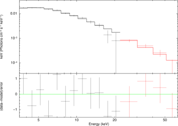
Figure 6: Upper panel: JEM-X (black) and ISGRI (red) spectra of 4U1323-619 in the energy range 3-65 keV. Lower panel: residuals in units of $\sigma$.

Table 5: Best-fit parameters of the spectral fitting on the JEM-X and ISGRI spectrum.

Component	Parameter	Value
Tabs	NH ($\times 10^{22}\rm cm^{-2}$)	4 (frozen)
nthComp	$\Gamma$	3.0${}^{+0.4}_{-0.5}$
nthComp	kTe (keV)	¿10
nthComp	kTbb (keV)	1.13${}^{+0.11}_{-0.15}$
nthComp	inp_type	0 (frozen)
nthComp	Redshift	0 (frozen)
nthComp	Norm. ($\times 10^{-3}$)	6.9${}^{+1.9}_{-1.3}$
	$\chi^{2}_{red}$(d.o.f.)	1.069(11)

5 Discussion

We estimated the orbital ephemeris of 4U 1323-619 using the whole available X-ray archival data from 1985 to 2011. We produced the linear and quadratic orbital ephemerides, finding that the value of the orbital period is 2.9419156(6) hrs. This is compatible with previous estimations (see Levine et al. 2011), but with an accuracy that is ten times higher than that proposed by Levine et al. (2011).
In a binary system the accretion of matter from the companion star onto the neutron star is the main mechanism of generation of radiation. The mass accretion rate, however, is governed by the angular momentum losses to which the binary system is subjected. The main channels of angular momentum loss are: the mass loss from the binary system as a consequence of the accretion, the generation of gravitational waves (especially in close binaries composed by massive stars), and the magnetic braking, which consists of a transfer of angular momentum from the companion star to the ionised matter that surrounds it and that interacts with its magnetic field. The redistribution of the angular momentum induced by these interactions causes a variation of the orbital period of the binary system. As a consequence of this, an estimation of the orbital period derivative is important to understand the orbital evolution of the system.
As a first step towards the extrapolation of an evolutive scenario for 4U 1323-619, we infer the companion star mass M₂. Assuming that 4U 1323-619 is a persistent X-ray source in a Roche lobe overflow regime, as suggested by the long time monitoring of the RXTE/ASM (see Fig. 7), then the companion star fills its Roche lobe and, consequently, the companion star radius R₂ is equal to the Roche lobe radius R_L2.
The Roche lobe radius is given by the expression

$$R_{L2}=0.46224\;a\left(\frac{m_{2}}{m_{1}+m_{2}}\right)^{1/3}$$ (5)

of Paczyński (1971), where $m_{1}$ and $m_{2}$ are the NS and companion star masses in units of solar masses and $a$ is the orbital separation of the binary system. Assuming that the companion star belongs to the lower main sequence, we adopt the relation

$$\frac{R_{2}}{R_{\odot}}=0.877\;m^{0.807}_{2},$$ (6)

valid for M-stars (Neece 1984). Combining equations 5 and 6 with the third Kepler law and assuming a neutron star (NS) mass of M₁=1.4 M_⊙ and the orbital period obtained from our ephemeris, we find that the companion star mass is M${}_{2}\simeq$0.28$\pm$0.03 M_⊙. Here we took into account an accuracy of 10% in the mass estimation (see Neece 1984). Our result is compatible with 0.25 M_⊙, as suggested by Zolotukhin et al. (2010). Since the companion star mass is 0.28 M_⊙ we expect that it is fully convective and, consequently, it cannot have a magnetic field anchored to it (Nelson & Rappaport 2003). This implies that magnetic braking as a driving mechanism of the orbital evolution is ruled out. Assuming that the unique mechanism of angular momentum loss in this binary system is due to the gravitational radiation and, considering a conservative mass transfer, we can infer the secular mass accretion rate by re-arranging Eq. 10 of Burderi et al. (2010), i.e.

$$\dot{m}_{-8}=0.6\;\frac{1}{3q-\frac{3}{2}n-\frac{5}{2}}\;m^{8/3}_{1}q^{2}(1+q)^{-1/3}P^{-8/3}_{2h},$$ (7)

where $\dot{m}_{-8}$ is the mass transfer rate from the companion star in units of $10^{-8}$ M_⊙ yr^-1, $q$ is the ratio of m₂ to m₁, and P_2h is the orbital period in units of two hours. The index $n$ can assume the values -1/3 or 0.8 and is associated with the internal structure of the companion star. If the star is in thermal equilibrium, its index $n$ is 0.8 (the index of the mass-radius relation we adopted in Eq. 6) whilst it is equal to the adiabatic index $n=-1/3$ otherwise. The values of $\dot{m}$ predicted by Eq. 7 are 6.4$\times 10^{-11}$ M_⊙ yr^-1 for $n$=0.8 and 1.42$\times 10^{-10}$ M_⊙ yr^-1 for $n$=-1/3.
Following the theory of secular evolution for X-ray binary systems, we can write the X-ray luminosity as

$$\begin{split}L=\frac{GM_{1}\dot{M}}{R_{1}}=&\\ 5.0\times 10^{37}\frac{1}{3q-\frac{3}{2}n-\frac{5}{2}}\;m^{11/3}_{1}q^{2}(1+q)^{-1/3}P^{-8/3}_{2h}{\rm erg\;s^{-1}}\end{split}$$ (8)

(see King 1988), where we substitute for $\dot{M}$ the expression of Eq. 7, and assume an NS radius $R_{1}$ of 10 km. Since we need to compare the predicted luminosity with the bolometric observed luminosity, we extrapolate the 0.5-100 keV luminosity from all the available observations. For some observations the spectral analysis of the source was already shown in literature. Since the energy spectrum in this case is dominated by a cut-off power-law component with a cut-off energy at 85 keV (Bałucińska-Church et al. 2009), we only use this spectral component to extrapolate the unabsorbed luminosity, using the photon index and normalisation values reported in literature for each observation and fixing the cut-off energy at 85 keV. We find a flux of 3.06$\times 10^{-10}$, 3.61$\times 10^{-10}$, 3.38$\times 10^{-10}$, and 3.62$\times 10^{-10}$ erg cm² s^-1 for the observations taken by Suzaku (Bałucińska-Church et al. 2009), EXOSAT (Parmar et al. 1989), BeppoSAX (Bałucińska-Church et al. 1999), and RXTE (Galloway et al. 2008), respectively. On the other hand, we extract a flux of 4.7$\times 10^{-10}$ erg cm² s^-1 in the 0.5-100 keV energy band from the XMM-Newton observation, and of 3.3$\times 10^{-10}$ erg cm² s^-1 from the JEM-X/ISGRI observation.
If we consider the 2-10 keV RXTE/ASM light curve spanning 15.5 years of data, from 3 March 1996 (10145 TJD) to 12 September 2011 (15816 TJD), we can observe that the source maintained a roughly constant count-rate (see Fig. 7). Fitting the ASM light curve with a constant function, in fact, we obtain a count rate of (0.483$\pm$0.011) c s^-1 with a $\chi^{2}(d.o.f.)=$5042(1388).
As a consequence of this, we estimate the mean flux for 4U 1323-619, averaging all the values of flux just obtained. The mean value of flux is of 3.6$\times 10^{-10}$ erg cm² s^-1. To be more conservative, we verified that this result is not sensitive to the specific value of N_H that was previously used for the JEM-X/ISGRI fit, which is the maximum available in literature. Adopting the minimum value of N_H available in literature (3.2$\times 10^{22}$ cm^-2; Bałucińska-Church et al. 2009), we extract a flux of 3.2$\times 10^{-10}$ erg cm² s^-1 for the JEM-X/ISGRI observation in the 0.5-100 keV energy band. Again, we obtain a mean value of flux of 3.6$\times 10^{-10}$ erg cm² s^-1 averaging all the values of flux obtained above.
Using the mean flux and adopting a distance of 10 kpc we determine a mean luminosity of (4.3 $\pm$ 0.4)$\times 10^{36}$ erg s^-1 for 4U 1323-619. In this estimation, we took into account an arbitrary error of 10%. We observe that the luminosity predicted by Eq. 8 can reach a maximum value of 1.7$\times 10^{36}$ erg s^-1 for n=-1/3, and a value of 7.5$\times 10^{35}$ erg s^-1 for n=0.8. We show the mean luminosity together with that predicted by Eq. 8 in the upper panel of Fig. 8. From this comparison, we can conclude that, for a distance of 10 kpc, the observed mean luminosity is not in accordance with that predicted by the theory of the secular evolution. We note that a wrong distance value could contribute to the observed inconsistency.

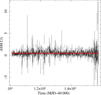
Figure 7: RXTE/ASM light curve in the 2-10 keV energy band. The red line represents the mean count rate maintained by 4U 1323-619 over 15.5 years. The bin time is four days.

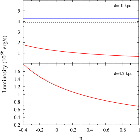
Figure 8: The red lines represent the luminosity as a function of the index $n$ for a distance of 10 kpc (upper panel) and 4.2 kpc (lower panel). The blue continuous lines represent the best values of the mean luminosity, while the dashed lines represent the associated errors.

For this purpose, we take into account the 3D extinction map of the radiation in the K_s band for our Galaxy (Marshall et al. 2006). This map suggests how great the extinction of the radiation is in the direction of the source ($l=307{}^{\circ}$, $b=0.5{}^{\circ}$) as a function of the distance. In Fig. 9 we report the extinction predicted by the model of Marshall et al. (2006) as a function of the distance from the source. We extrapolated the profile, taking into account the galactic coordinates of 4U 1323-619. We calculate the visual extinction using the Güver & Özel (2009) relation

$$N_{H}=(2.21\pm 0.09)\times 10^{21}A_{V},$$ (9)

where N_H is the equivalent column density of neutral hydrogen of the absorbing interstellar matter and A_V is the visual extinction of the source radiation. Using the N_H value 3.2$\times 10^{22}$ cm^-2 found by Bałucińska-Church et al. (2009), we estimate a visual extinction of A_V=14.5$\pm$0.7 mag that is compatible with the value found by Bałucińska-Church et al. (1999).

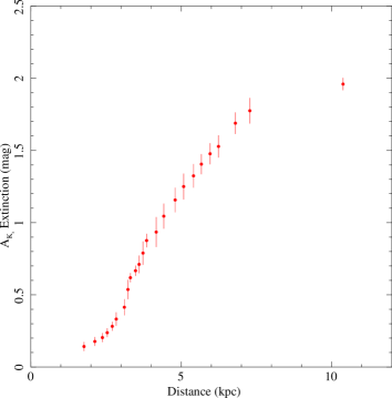
Figure 9: Extinction of the K_s radiation in the direction of the source ($l=307{}^{\circ}$ , $b=0.5{}^{\circ}$) as a function of the distance (Marshall et al. 2006).

The visual extinction is related to the extinction of the radiation in the K_s band through the relation

$$A_{K_{S}}=(0.062\pm 0.005)\;A_{V}\;{\rm mag}$$ (10)

(Nishiyama et al. 2008), where A${}_{K_{S}}$ is the extinction in the K_S band. With this relation we find a value for the extinction of A${}_{K_{S}}$= 0.90$\pm$0.09 mag.
We fitted the profile of the extinction of Fig. 9 with a quadratic function between 3 and 6 kpc, imposing a null value of the extinction for a null distance. The fit gives us a $\chi^{2}_{red}$ of 1.38 with 12 degrees of freedom, a linear parameter of 0.10$\pm$ 0.02, and a quadratic parameter of 0.028$\pm$0.004. The uncertainties are given with a confidence level of 68%. According to the value of A${}_{K_{S}}$, obtained before, we estimate a distance of 4.2${}^{+0.8}_{-0.7}$ kpc with a confidence level of 68%. This distance is fully in agreement with the value of distance suggested by Zolotukhin et al. (2010).
Taking into account a distance of 4.2${}_{-0.7}^{+0.8}$ kpc, we infer a luminosity of (0.8 $\pm$ 0.3)$\times 10^{36}$ erg s^-1 that is compatible with the one predicted by Eq. 8 for a $n$ index close to 0.8 and thus for a thermal equilibrium state of the companion star (see Fig. 8).
A value of luminosity that completely matches the one predicted by Eq. 8 for $n$=0.8 is obtained for a distance to the source of d$\sim$4.17 kpc. According to the Marshall et al. (2006) model (see Fig. 9), an extinction of 0.88 mag competes for this value of distance in the K_s band, and thus, by Eq. 10 and Eq. 9, we infer A_v=14.2 mag and N${}_{H}\sim$3.1$\times 10^{22}$ cm^-2. This value of N_H is fully in agreement with that obtained by Bałucińska-Church et al. (2009).
We also explored a non-conservative mass transfer scenario. We observe that in the case in which the mass is expelled from the position of the companion star, for an index n=0.8 and a distance from the source of 4.2 kpc, the luminosities obtained from the individual X-ray observations are compatible with the luminosity predicted by a non-conservative mass transfer theory for a value of $\beta\geq$ 0.8, where $\beta$ is the fraction of matter accreted onto the neutron star. This implies that the observations are in agreement with a scenario in which more than the 80% of the mass is accreted onto the neutron star. Thus, on the basis of the fact that only the 20% of mass of the companion star is lost from the system, we can confirm that the mass accretion mechanism could be rightly considered conservative.
To investigate the orbital evolution of the system, we need to compare the Kelvin-Helmholtz time-scale $\tau_{KH}$ (i.e. the characteristic time to reach the thermal equilibrium for a star) with the mass transfer time-scale $\tau_{\dot{M}}$. We calculate the Kelvin-Helmholtz time-scale adopting the relation

$$\tau_{KH}=3.1\times 10^{7}\left(\frac{M_{2}}{M_{\odot}}\right)^{2}\frac{R_{\odot}}{R_{2}}\frac{L_{\odot}}{L}$$ (11)

of Verbunt (1993), together with the mass-luminosity relation for a M-type star

$$\frac{L_{2}}{L_{\odot}}=0.231\;\left(\frac{M_{2}}{M_{\odot}}\right)^{2.61}$$ (12)

of Neece (1984). Moreover, we assume the Neece (1984) mass-radius relation of Eq. 6 for a main sequence M-type star in equilibrium. Our estimation of the Kelvin-Helmholtz time-scale is of $\tau_{KH}$=9$\times 10^{8}$ yrs.
On the other hand, we extrapolate the mass transfer time-scale using the relation

$$\tau_{\dot{M}}=\frac{m_{2}}{\dot{m}}=\frac{G\;m_{1}m_{2}}{L\;R_{NS}},$$ (13)

where $L$ is the source luminosity. To achieve this, we use the mean luminosity estimated above during the ASM monitoring, obtaining a mass transfer time-scale of 4.4$\times 10^{9}$ yrs. This value is greater than the Kelvin-Helmholtz time-scale by a factor of 4.9. This implies that the companion star is in thermal equilibrium and we can conclude that the mass-radius relation in Eq. 6 has been correctly used, suggesting that the proposed scenario is self-consistent.
To understand how the binary system is going to evolve, we estimate the orbital period derivative re-arranging Eq. 4 of Burderi et al. (2010):

$$\dot{m}_{-8}=87.5\;(3n-1)^{-1}m_{2}\left(\frac{\dot{P}_{-10}}{P_{2h}}\right),$$ (14)

where $\dot{P}_{-10}$ is the orbital period derivative in units of 10^-10 s/s and $P_{2h}$ is the orbital period of the system in units of two hours. Adopting an index n=0.8, we obtain a value of the period derivative of $\dot{P}\sim-5.4\times 10^{-14}$ s/s that is compatible with the constraint on the $\dot{P,}$ which is estimated from our ephemeris, i.e. $(0.8\pm 1.3)\times 10^{-11}$ s/s. From this result, we can infer that the orbital period is decreasing and that the system is shrinking as a consequence of the orbits being Keplerian.

6 Conclusions

We constrain the X-ray source position of 4U 1323-619, finding out that the source is located inside a circular area centred at RA (J2000)= 201.6543^∘ and DEC (J2000)= -62.1358^∘ and with a radius of 0.0002^∘ (that is 0.6”). This result allows us to confirm the suggestion of Zolotukhin et al. (2010) that the B source in Fig. 1 is the IR counterpart of 4U 1323-619.
In addition, using observations from 1985 to 2011, we infer for the first time the linear and quadratic orbital ephemerides for 4U 1323-619. We estimate the orbital period of the binary system with an accuracy ten times higher than that which was proposed by Levine et al. (2011). We obtain a refined measure of the period of $P=2.9419156(6)$ hrs, in line with previous estimates, as reported in the literature. We infer for the first time a weak constraint on the orbital period derivative of the system that is of $\dot{P}=(8\pm 13)\times 10^{-12}$ s/s. Assuming a fully conservative mass-transfer scenario and that the companion star is an M-type main-sequence star, we estimate the mass of the companion to be of 0.28$\pm$0.03 M_⊙. This result suggests that the star is fully convective and that the magnetic braking mechanism can be ruled out as an explanation of angular momentum losses from the binary system, which is therefore driven by the mechanism of gravitational radiation.
We inferred that the companion star transfers matter onto the neutron star surface via the inner Lagrangian point in a conservative regime. According to the conservative mass-transfer scenario, and taking into account the map of the K_s radiation extinction in our Galaxy, we estimate a distance of (4.2${}^{+0.8}_{-0.7}$) kpc at 68% confidence level.

References

- Arnaud (1996) Arnaud, K. A. 1996, in Astronomical Society of the Pacific Conference Series, Vol. 101, Astronomical Data Analysis Software and Systems V, ed. G. H. Jacoby & J. Barnes, 17
- Asplund et al. (2009) Asplund, M., Grevesse, N., Sauval, A. J., & Scott, P. 2009, ARA&A, 47, 481
- Bałucińska-Church et al. (1999) Bałucińska-Church, M., Church, M. J., Oosterbroek, T., et al. 1999, A&A, 349, 495
- Bałucińska-Church et al. (2009) Bałucińska-Church, M., Dotani, T., Hirotsu, T., & Church, M. J. 2009, A&A, 500, 873
- Boirin et al. (2005) Boirin, L., Méndez, M., Díaz Trigo, M., Parmar, A. N., & Kaastra, J. S. 2005, A&A, 436, 195
- Burderi et al. (2010) Burderi, L., Di Salvo, T., Riggio, A., et al. 2010, A&A, 515, A44
- Courvoisier et al. (2003) Courvoisier, T. J.-L., Walter, R., Beckmann, V., et al. 2003, A&A, 411, L53
- Forman et al. (1978) Forman, W., Jones, C., Cominsky, L., et al. 1978, ApJS, 38, 357
- Frank et al. (1987) Frank, J., King, A. R., & Lasota, J.-P. 1987, A&A, 178, 137
- Galloway et al. (2008) Galloway, D. K., Muno, M. P., Hartman, J. M., Psaltis, D., & Chakrabarty, D. 2008, ApJS, 179, 360
- Güver & Özel (2009) Güver, T. & Özel, F. 2009, MNRAS, 400, 2050
- Iaria et al. (2014) Iaria, R., Di Salvo, T., Burderi, L., et al. 2014, A&A, 561, A99
- Iaria et al. (2015) Iaria, R., Di Salvo, T., Gambino, A. F., et al. 2015, A&A, 582, A32
- King (1988) King, A. R. 1988, QJRAS, 29, 1
- Lebrun et al. (2003) Lebrun, F., Leray, J. P., Lavocat, P., et al. 2003, A&A, 411, L141
- Levine et al. (2011) Levine, A. M., Bradt, H. V., Chakrabarty, D., Corbet, R. H. D., & Harris, R. J. 2011, ApJS, 196, 6
- Lund et al. (2003) Lund, N., Budtz-Jørgensen, C., Westergaard, N. J., et al. 2003, A&A, 411, L231
- Marshall et al. (2006) Marshall, D. J., Robin, A. C., Reylé, C., Schultheis, M., & Picaud, S. 2006, A&A, 453, 635
- Neece (1984) Neece, G. D. 1984, ApJ, 277, 738
- Nelson & Rappaport (2003) Nelson, L. A. & Rappaport, S. 2003, ApJ, 598, 431
- Nishiyama et al. (2008) Nishiyama, S., Nagata, T., Tamura, M., et al. 2008, ApJ, 680, 1174
- Paczyński (1971) Paczyński, B. 1971, ARA&A, 9, 183
- Parmar et al. (1989) Parmar, A. N., Gottwald, M., van der Klis, M., & van Paradijs, J. 1989, ApJ, 338, 1024
- Predehl & Schmitt (1995) Predehl, P. & Schmitt, J. H. M. M. 1995, A&A, 293, 889
- Smale (1995) Smale, A. P. 1995, AJ, 110, 1292
- van der Klis et al. (1985) van der Klis, M., Jansen, F., van Paradijs, J., & Stollman, G. 1985, Space Sci. Rev., 40, 287
- Verbunt (1993) Verbunt, F. 1993, ARA&A, 31, 93
- Verner et al. (1996) Verner, D. A., Ferland, G. J., Korista, K. T., & Yakovlev, D. G. 1996, ApJ, 465, 487
- Warwick et al. (1981) Warwick, R. S., Marshall, N., Fraser, G. W., et al. 1981, MNRAS, 197, 865
- Zolotukhin et al. (2010) Zolotukhin, I. Y., Revnivtsev, M. G., & Shakura, N. I. 2010, MNRAS, 401, L1