Two-photon Rabi model: Analytic solutions and spectral collapse

Abstract

The two-photon quantum Rabi model with quadratic coupling is studied using extended squeezed states and we derive $G$-functions for Bargmann index $q=1/4$ and $3/4$. The simple singularity structure of the $G$-function allows to draw conclusions about the distribution of eigenvalues along the real axis. The previously found picture of the spectral collapse at critical coupling $g_{\mathrm{c}}$ has to be modified regarding the low lying states, especially the ground state: We obtain a finite gap between ground state and the continuum of excited states at the collapse point. For large qubit splitting, also other low lying states may be separated from the continuum at $g_{\mathrm{c}}$. We have carried out a perturbative analysis allowing for explicit and simple formulae of the eigenstates. Interestingly, a vanishing of the gap between ground state and excited continuum at $g_{\mathrm{c}}$ is obtained in each finite order of approximation. This demonstrates cleary the non-pertubative nature of the excitation gap. We corroborate these findings with a variational calculation for the ground state.

Keywords Two-photon Rabi model, extended squeezed states, analytic solutions

1 Introduction

The quantum Rabi model (QRM), a major paradigm for light-matter interaction since its inception in 1936 [1], has drawn persistent attention due to its applications in numerous fields ranging from quantum optics to condensed matter physics and even, very recently, to quantum information science. It describes a two-level system (qubit) coupled linearly to a cavity electromagnetic mode [1, 2]. The Hamiltonian can be written as

$$H_{\mathrm{R}}=\frac{\Omega}{2}\sigma_{z}+\omega a^{\dagger}a+g(a^{\dagger}+a)\sigma_{x},$$ (1)

where $\sigma_{x,z}$ are Pauli matrices describing the two-level system and $a$ ($a^{\dagger}$) are the annihilation (creation) bosonic operators of the cavity mode. Although it appears to be much simpler than the hydrogen atom, it has been considered unsolvable for a long time. Recently, by using Bargmann-space methods [4], it was shown that this model is not only exactly solvable but also integrable [5]. The so-called regular spectrum can be obtained by zeros of a function $G_{\mathrm{R}}(E)$, i.e. $G_{\mathrm{R}}(E_{n})=0$ entails $E_{n}\in\mathrm{spec}(H_{\mathrm{R}})$. This $G$-function can be written explicitly in terms of confluent Heun functions [6]. $G_{\mathrm{R}}(E)$ was then recovered within the extended coherent states approach, which avoids the mapping into the Bargmann space of analytic functions [7]. These results have stimulated extensive research in the QRM and related models [8, 9, 10, 11, 12, 13, 14, 15, 16, 17, 18, 19, 20].

On the other hand, the two-photon QRM has also attracted a lot of attention. It couples the two-level system to the cavity mode non-linearly and describes a three-level system when the third state can be adiabatically eliminated. It may be realized for Rydberg atoms in microwave superconducting cavities [21, 22] and quantum dots [23, 24] . The two-photon QRM has also been studied for a long time both with the RWA [25] and beyond the RWA [26, 27, 28]. Recently, a realistic implementation of two-photon quantum Rabi models using trapped ions has been proposed [29], which could reach the coupling region corresponding to the interaction-induced spectral collapse. This feature can only be observed in the deep strong coupling regime of the quantum Rabi model [30] and resembles in this respect the well-known superradiant phase transition of the Dicke model [31].

2 Exact solution using the $\bm{SU(1,1)}$ algebraic structure

The Hamiltonian of the two-photon QRM is given by

$$H=-\frac{\Omega}{2}\sigma_{x}+a^{\dagger}a+g\left[\left(a^{\dagger}\right)^{2}+a^{2}\right]\sigma_{z},$$ (2)

where $\Omega$ is the qubit splitting, $a^{\dagger}$ $\left(a\right)$ is the photonic creation (annihilation) operator of the single-mode cavity with frequency $\omega=1$. We have used the “spin-boson” representation [32], exchanging $\sigma_{x}$ and $\sigma_{z}$. The interaction part is quadratic in the boson operators, while in the original QRM it is linear (see (1)).

In this section we derive the G-function found previously for this model [7] in a more concise and compact way. First, we perform a Bogoliubov transformation

$$b=ua+va^{\dagger},\qquad b^{\dagger}=ua^{\dagger}+va,$$ (3)

to a new bosonic operators. With

$$u=\sqrt{\frac{1+\beta}{2\beta}},\qquad v=\sqrt{\frac{1-\beta}{2\beta}},$$ (4)

and $\beta=\sqrt{1-4g^{2}}$, the upper diagonal matrix element of the Hamiltonian becomes

$$H_{11}=a^{\dagger}a+g\left[\left(a^{\dagger}\right)^{2}+a^{2}\right]=\frac{b^{\dagger}b-v^{2}}{u^{2}+v^{2}}.$$

In terms of $b,b^{\dagger}$, the Hamiltonian reads

$$H=\left(\begin{array}[]{ll}\frac{b^{\dagger}b-v^{2}}{u^{2}+v^{2}}&~{}-\frac{\Omega}{2}\\ ~{}~{}-\frac{\Omega}{2}&\;\;\;H_{22}\end{array}\right),$$ (5)

with

$$H_{22}=\left(u^{2}+v^{2}+4guv\right)b^{\dagger}b-2uv\left[\left(b^{\dagger}\right)^{2}+b^{2}\right]+2guv+v^{2}.$$

The operators $b^{\dagger}b$, $(b^{\dagger})^{2}$, $b^{2}$ provide a representation of the non-compact Lie algebra $su(1,1)$: With

$$K_{0}=\frac{1}{2}\left(b^{\dagger}b+\frac{1}{2}\right),\qquad K_{+}=\frac{1}{2}\left(b^{\dagger}\right)^{2},\qquad K_{-}=\frac{1}{2}b^{2},$$

we have

$$\left[K_{0},K_{\pm}\right]=\pm K_{\pm},\qquad\left[K_{+},K_{-}\right]=-2K_{0}.$$

The quadratic Casimir operator $C$ of the algebra is given by

$$C=K_{+}K_{-}-K_{0}\left(K_{0}-1\right).$$

The infinite-dimensional unitary representations of $su(1,1)$ are labeled by the value $q$ of $C$, the Bargmann index. Here, the Hilbert space $\cal H$ generated by $b^{\dagger}$ on the state $|0\rangle_{\mathrm{b}}$ anihilated by $b$, separates into two $H$-invariant subspaces, ${\cal H}={\cal H}_{\frac{1}{4}}\oplus{\cal H}_{\frac{3}{4}}$ for $q=\frac{1}{4},\frac{3}{4}$. A basis of ${\cal H}_{q}$ is given by the normalized states

$$\left|q,n\right\rangle_{\mathrm{b}}=\frac{\left(b^{\dagger}\right)^{2\left(n+q-\frac{1}{4}\right)}}{\sqrt{\left[2\left(n+q-\frac{1}{4}\right)\right]!}}\left|0\right\rangle_{\mathrm{b}}=\left|2\left(n+q-\frac{1}{4}\right)\right\rangle_{\mathrm{b}},$$ (6)

$$q=\frac{1}{4},\frac{3}{4},\qquad n=0,1,2,...\infty.$$

The operators satisfy

$$K_{+}\left|q,n\right\rangle_{\mathrm{b}}=\sqrt{\left(n+q+\frac{3}{4}\right)\left(n+q+\frac{1}{4}\right)}\left|q,n+1\right\rangle_{\mathrm{b}},$$

$$K_{-}\left|q,n\right\rangle_{\mathrm{b}}=\sqrt{\left(n+q-\frac{1}{4}\right)\left(n+q-\frac{3}{4}\right)}\left|q,n-1\right\rangle_{\mathrm{b}},$$

$$K_{0}\left|q,n\right\rangle_{\mathrm{b}}=\left(n+q\right)\left|q,n\right\rangle_{\mathrm{b}}.$$

Note that the vacuum with respect to the original boson operators $a,a^{\dagger}$, $|0\rangle_{\mathrm{a}}$, with the property $a|0\rangle_{\mathrm{a}}=0$, may be expressed in terms of $\left|\frac{1}{4},n\right\rangle_{\mathrm{b}}$ as

$$\left|0\right\rangle_{\mathrm{a}}=\sum_{n=0}^{\infty}z_{n}^{(\frac{1}{4})}\left|\frac{1}{4},n\right\rangle_{\mathrm{b}},$$

because the decomposition ${\cal H}={\cal H}_{\frac{1}{4}}\oplus{\cal H}_{\frac{3}{4}}$ is left invariant by the Bogoliubov transformation (3). We can write therefore $|0\rangle_{\mathrm{a}}=|\frac{1}{4},0\rangle_{\mathrm{a}}$. The condition $a\left|0\right\rangle_{\mathrm{a}}=0,$ leads to

$$z_{n}^{(\frac{1}{4})}\varpropto\frac{\sqrt{\left(2n\right)!}}{n!}\left(\frac{v}{2u}\right)^{n}.$$ (7)

The lowest lying state (with respect to the $a$-operators) in ${\cal H}_{\frac{3}{4}}$ reads then

$$\left|\frac{3}{4},0\right\rangle_{\mathrm{a}}=a^{\dagger}\left|\frac{1}{4},0\right\rangle_{\mathrm{a}}=\left(ub^{\dagger}-vb\right)\sum_{n=0}^{\infty}z_{n}^{(\frac{1}{4})}\left|\frac{1}{4},n\right\rangle_{\mathrm{b}}=\sum_{n=0}^{\infty}z_{n}^{(\frac{3}{4})}\left|\frac{3}{4},n\right\rangle_{\mathrm{b}},$$

where

$$z_{n}^{(\frac{3}{4})}\varpropto\frac{\sqrt{\left(2n+1\right)!}}{n!}\left(\frac{v}{2u}\right)^{n}.$$ (8)

In summary,

$$z_{n}^{(q)}\varpropto\frac{\sqrt{\left[2\left(n+q-\frac{1}{4}\right)\right]!}}{n!}\left(\frac{v}{2u}\right)^{n}.$$ (9)

In terms of the $K_{0}$, $K_{\pm}$, the Hamiltonian reads

$$H=\left(\begin{array}[]{ll}\frac{\left(2K_{0}-\frac{1}{2}\right)-v^{2}}{u^{2}+v^{2}}&~{}-\frac{\Omega}{2}\\ ~{}~{}-\frac{\Omega}{2}&\;\;\;H_{22}^{\prime}\end{array}\right),$$ (10)

where

$$H_{22}^{\prime}=\left(u^{2}+v^{2}+4guv\right)\left(2K_{0}-\frac{1}{2}\right)-4uv\left(K_{+}+K_{-}\right)+2guv+v^{2}.$$

An eigenfunction $|\psi,E\rangle$ of $H$ with eigenvalue $E$ may be expanded in terms of the $b$-operators as

$$\left|\psi,E\right\rangle=\left(\ \begin{array}[]{l}\sum_{m=0}^{\infty}\sqrt{\left[2\left(m+q-\frac{1}{4}\right)\right]!}e_{m}^{(q)}\left|q,m\right\rangle_{\mathrm{b}}\\ \sum_{m=0}^{\infty}\sqrt{\left[2\left(m+q-\frac{1}{4}\right)\right]!}f_{m}^{(q)}\left|q,m\right\rangle_{\mathrm{b}}\end{array}\right),$$ (11)

Projecting both sides of the Schrödinger equation onto ${}_{\mathrm{b}}\left\langle q,n\right|$ gives a linear relation between coefficients $e_{n}^{(q)}$ and $f_{n}^{(q)}$,

$$e_{n}^{(q)}=\frac{\frac{\Omega}{2}}{\frac{2\left(n+q-\frac{1}{4}\right)-v^{2}}{u^{2}+v^{2}}-E}f_{n}^{(q)},$$ (12)

and

$$8uv\left(n+q+\frac{3}{4}\right)\left(n+q+\frac{1}{4}\right)f_{n+1}^{(q)}=-2uvf_{n-1}^{(q)}$$ (13)

$$+\left[\left(u^{2}+v^{2}+4guv\right)\left(2\left(n+q\right)-\frac{1}{2}\right)+2guv+v^{2}-E\right]f_{n}^{(q)}-\frac{\Omega}{2}e_{n}^{(q)}.$$

We obtain a three-term recurrence relation

$$f_{n+1}^{(q)}=\frac{\left(1+4g^{2}\right)\left(n+q\right)-\beta^{2}\left(x+q\right)-\frac{\Omega^{2}}{16\left(n-x\right)}}{4g\left(n+q+\frac{3}{4}\right)\left(n+q+\frac{1}{4}\right)}f_{n}^{(q)}-\frac{f_{n-1}^{(q)}}{4\left(n+q+\frac{3}{4}\right)\left(n+q+\frac{1}{4}\right)},$$ (14)

where $x=\frac{E}{2\beta}+\frac{v^{2}}{2}-q+\frac{1}{4}$, the coefficients $f_{n}^{(q)}$ are calculated with initial conditions $f_{0}^{(q)}=1$, $f_{-1}^{(q)}=0$.

Because of parity invariance in each space ${\cal H}_{q}$ [7], projecting the wavefunction $|\psi,E\rangle$ onto $|\uparrow\rangle|q,0\rangle_{\mathrm{a}}$ and $|\downarrow\rangle|q,0\rangle_{\mathrm{a}}$ respectively, we can define the two-photon G-function as

$$G_{\pm}^{(q)}(x)=\sum_{n=0}^{\infty}f_{n}^{(q)}\;\left[1+\Pi\frac{\Omega}{4\beta\left(n-x\right)}\;\right]\frac{\left[2\left(n+q-\frac{1}{4}\right)\right]!}{n!}\left(\frac{v}{2u}\right)^{n},$$ (15)

where $\Pi=\pm 1$, corresponding to positive(negative) parity. So far, we have just re-derived the $G$-function in a more compact and concise way compared to [7]

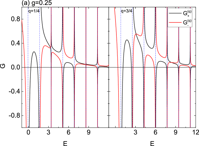
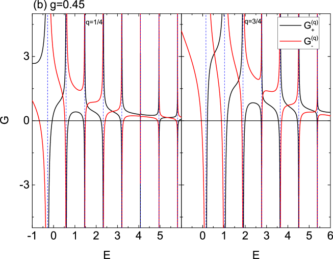
Figure 1: (Color online) G curves for the two-photon QRM at $\Omega=1$, (a) $g=0.25$ (upper) and (b) $g=0.45$ (lower).

We plot the two-photon $G$-function in figure 1 for $\Omega=1$, two values of $g$, $0.25$ and $0.45$, and both Bargmann indices $q=\frac{1}{4}$ and $\frac{3}{4}$. The zeros give the location of the energy spectrum, which is plotted in figure 2 as function of $g$.

The poles in figure 1 correspond to values of $E=\beta\left(2(n+q-\frac{1}{4})-v^{2}\right)=2\beta(n+q)-\frac{1}{2}$. The position of the first pole corresponds to $E=2\beta q-\frac{1}{2}$. The distance between adjacent poles is $2\beta$ and vanishes as $g\rightarrow\frac{1}{2}=g_{\mathrm{c}}$. Therefore zeros of $G_{\pm}^{(q)}(E)$ (energy levels) between two poles will collapse towards $-\frac{1}{2}$ when $g\rightarrow\frac{1}{2}$, as shown in figure 2.

3 Spectral collapse and energy gap

The energy of the ground state does not tend to $-\frac{1}{2}$ when $g\rightarrow\frac{1}{2}$, in sharp contrast with almost all of the excited states. This is seen in all previous numerical calculations of the spectra, but has never been discussed in detail. Here, we will present an explanation with help of the analytical exact solutions.

The first pole ($n=0$) of $G_{\pm}^{(q)}(E)$ forms the zeroth baseline in the spectral graph,

$$E_{\mathrm{pol}}^{(1)}(g)=2\sqrt{1-4g^{2}}q-\frac{1}{2}$$ (16)

and approaches $2q-\frac{1}{2}$ in the weak coupling limit $g\rightarrow 0$. On the other hand, for $g=0$, the qubit is decoupled from the cavity, all eigenenergies are easily obtained as

$$E^{n}_{\Pi}(g=0)=\Pi\frac{\Omega}{2}\left(-1\right)^{n}+2\left(n+q-\frac{1}{4}\right)$$ (17)

where $n=0,1,2,3...$. If $E^{n}_{\Pi}(g=0)<E_{\mathrm{pol}}^{(1)}(g=0)$, i.e.

$$n<-\Pi\frac{\Omega}{4}(-1)^{n},\qquad n=0,1,2,...$$ (18)

then the energy level $E^{n}_{\Pi}(g)$ will be smaller than $E^{(1)}_{\mathrm{pol}}(g)$ for $g>0$ as well until an exceptional solution [5] is reached where the pole coincides with an energy eigenvalue and the zeroth baseline is crossed. This is possible if the exceptional solution is not Juddian (doubly-degenerate) [32, 33, 34]. We shall see that also the opposite occurs: an energy level above the first pole for small $g$ crosses the zeroth baseline at $g_{0}$ and lies below the first pole for $g>g_{0}$. These levels correspond to zeros of the $G-$function which are not pinched between the poles as $g$ approaches $g_{\mathrm{c}}=\frac{1}{2}$ and will therefore not collapse into the continuum.

The ground state belongs to negative parity for each $q$ and does not cross the zeroth baseline for the examples in figure 2. It will always be separated by a finite gap from the continuum at $g=\frac{1}{2}$. For large $\Omega=3$, we have in the lower panels of figure 2 an example of an excited state with positive parity crossing the zeroth baseline at $g_{0}<g_{\mathrm{c}}$. This state will also not collapse as $g=\frac{1}{2}$ is reached. Because several eigenstates for each parity are located below the first pole for small $g$ according to 18, and correspond to zeros of the $G$-function in a pole-free region, none of them is constrained by the argument above and may be separated from the continuum at the critical coupling, if they do not cross the zeroth baseline for some $g<g_{\mathrm{c}}$.

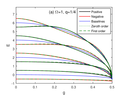
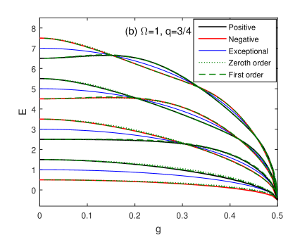
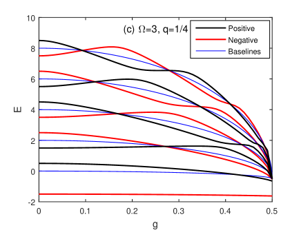
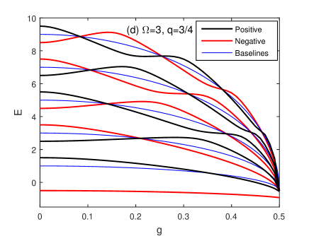
Figure 2: (Color online) Energy spectra obtained from G-function for $\Omega=1$ (upper panel) and $\Omega=3$ (low panel), $q=1/4$ ( left panel) and $q=3/4$ (right panel). The baselines (blue solid) are also presented. The zeroth order approximation (dotted) and first order approximation (dashed) are given only for $\Omega=1$ (upper panel).

4 Finite-dimensional approximations

Similar to $b$ and $b^{{\dagger}}$, we can introduce another set of operators

$$c=ua-va^{\dagger},\qquad c^{\dagger}=ua^{\dagger}-va,$$ (19)

which removes the terms $a^{2}$, $(a^{\dagger})^{2}$ in the other diagonal element of the Hamiltonian matrix element

$$H_{22}=a^{\dagger}a-g\left[\left(a^{\dagger}\right)^{2}+a^{2}\right]=\frac{c^{\dagger}c-v^{2}}{u^{2}+v^{2}}.$$

The corresponding basis reads

$$\left|q,n\right\rangle_{\mathrm{c}}=\frac{\left(c^{\dagger}\right)^{2\left(n+q-\frac{1}{4}\right)}}{\sqrt{\left[2\left(n+q-\frac{1}{4}\right)\right]!}}\left|0\right\rangle_{\mathrm{c}}=\left|2\left(n+q-\frac{1}{4}\right)\right\rangle_{\mathrm{c}},$$ (20)

$$q=\frac{1}{4},\frac{3}{4},\qquad n=0,1,2,....\infty,$$

The Hamiltonian reads in terms of $b$ and $c$ operators

$$H=\left(\begin{array}[]{ll}\beta\left(b^{\dagger}b-v^{2}\right)&~{}-\frac{\Omega}{2}\\ ~{}~{}-\frac{\Omega}{2}&\;\beta\left(c^{\dagger}c-v^{2}\right)\end{array}\right),$$ (21)

For each parity $\Pi$ we write the wavefunction as

$$\left|\psi,E\right\rangle_{q}=\left(\ \begin{array}[]{l}\sum_{n=0}^{\infty}u_{n}^{(q)}\left|q,n\right\rangle_{\mathrm{b}}\\ -\Pi\sum_{n=0}^{\infty}\left(-1\right)^{n}u_{n}^{(q)}\left|q,n\right\rangle_{\mathrm{c}}\end{array}\right).$$ (22)

From the Schrödinger equation it follows then

$$\beta\left(b^{\dagger}b-v^{2}\right)\sum_{n=0}^{\infty}u_{n}^{(q)}\left|q,n\right\rangle_{\mathrm{b}}+\Pi\frac{\Omega}{2}\sum_{n=0}^{\infty}\left(-1\right)^{n}u_{n}^{(q)}\left|q,n\right\rangle_{\mathrm{c}}=E\sum_{n=0}^{\infty}u_{n}^{(q)}\left|q,n\right\rangle_{\mathrm{b}}.$$

Projection on $\left|q,m\right\rangle_{\mathrm{b}}$ gives

$$\beta\left(2(m+q-\frac{1}{4})-v^{2}\right)u_{m}^{(q)}+\Pi\sum_{n=0}^{\infty}u_{n}^{(q)}\ D_{m,n}^{(q)}=Eu_{m}^{(q)}$$ (23)

with

$$D_{m,n}^{(q)} =\frac{\Omega}{2}\left(-1\right)^{n}\ _{\mathrm{b}}\left\langle q,m\right|\left.q,n\right\rangle_{\mathrm{c}}$$ (24)

$$=\frac{\Omega}{2}\ \left(-1\right)^{m}\beta^{\frac{1}{2}}\sqrt{\frac{\left[2\left(n+q-\frac{1}{4}\right)\right]!}{\left[2\left(m+q-\frac{1}{4}\right)\right]!}}P_{m+n+2\left(q-\frac{1}{4}\right)}^{m-n}\left(\beta\right)$$

where $P_{m+n}^{m-n}\left(\beta\right)$ is an associated Legendre polynomial, which is defined for all values of integer $\ m$ and $n$. Obviously, when $g\rightarrow\frac{1}{2}$, $D_{mn}\rightarrow 0,$ which will be used later.

We can use the set of equations from (23) to diagonalize the Hamiltonian and get numerical exact solutions with some truncation in $n$. We define the $N$-th order approximation by selecting $N$ coefficients $u_{n}^{(q)}$, $\left(n=m,m+1,...,m+N\right)$ in the (23) and neglect the other terms.

In zeroth order, we set $N=0$ and have

$$\beta\left(2(m+q-\frac{1}{4})-v^{2}\right)u_{m}^{(q)}+\Pi u_{m}^{(q)}\ D_{m,m}^{(q)}=Eu_{m}^{(q)}$$ (25)

which gives the eigenenergy immediately

$$E_{m}^{(0)}\left(\Pi\right)=\beta\left(2(m+q-\frac{1}{4})-v^{2}\right)+\Pi D_{m,m}^{(q)}$$ (26)

The ground-state energy is $E_{0}^{(0)}\left(\Pi=-1\right)$, of negative parity.

For the $N=1$ we obtain an explicit expression for the energy as well. For the excited states, we have two equations for two coefficients

$$\left[\beta\left(2(m+q-\frac{1}{4})-v^{2}\right)+\Pi D_{m,m}^{(q)}\right]u_{m}^{(q)}+\Pi u_{m+1}^{(q)}\ D_{m,m+1}^{(q)}=Eu_{m}^{(q)},$$ (27)

$$\Pi D_{m+1,m}^{(q)}u_{m}^{(q)}+\left[\beta\left(2(m+q+\frac{3}{4})-v^{2}\right)+\Pi D_{m+1,m+1}^{(q)}\right]u_{m+1}^{(q)}=Eu_{m+1}^{(q)}.$$ (28)

Obviously, for each $m=0,1,2,...$, we have four solutions from the above equation, two of them are redundant. At weak coupling, the parity for each eigenstate is fixed: even $m$ for positive parity and odd $m$ for negative parity. It follows $\Pi\left(-1\right)^{m}=1$. Therefore, we may replace $\Pi$ by $(-1)^{m}$ and obtain for the eigenenergies of the excited states

$$E_{m}^{(1)}=\beta\left(2(m+q+\frac{1}{4})-v^{2}\right)+\frac{(-1)^{m}}{2}(D_{m,m}+D_{m+1,m+1})$$

$$\pm\frac{1}{2}\sqrt{\left[(-1)^{m}(D_{m,m}-D_{m+1,m+1})-2\beta\right]^{2}+4D_{m,m+1}^{2}},m=0,1,2,...$$ (29)

Note that for each $m$, we have two solutions with the same parity.

The ground-state energy in the first order approximation is given by (27) and (28) for$\ m=0,q=\frac{1}{4}$, and $\Pi=-1$

$$E_{\mathrm{GS}}^{(1)}=-\frac{1}{2}+\frac{3}{2}\beta-\frac{1}{2}\left(\ D_{0,0}^{(\frac{1}{4})}+\ D_{1,1}^{(\frac{1}{4})}\right)-\frac{1}{2}\sqrt{\left(D_{1,1}^{(\frac{1}{4})}-\ D_{0,0}^{(\frac{1}{4})}-2\beta\right)^{2}+4D_{1,0}^{(\frac{1}{4})}\ D_{0,1}^{(\frac{1}{4})}}.$$ (30)

The arbitrary $N$-th order approximation can be performed straightforwardly. There are $2\left(N+1\right)$ solutions for each value of $m$.

The energy levels in zeroth order and first order approximation are also presented in figure 2 ($\Omega=1$, upper level). The energy levels agree even in the zero order approximation quite well with the exact ones. Interestingly, the spectral collapse is exhibited already in zeroth order. This is not strange, because the matrix elements $D_{mn}$ in (23) tends to zero if $g$ approaches $\frac{1}{2}$. Actually in any order of the analytic approximation, the energy for all eigenstates approaches $-\frac{1}{2}$, including the ground state, leading to a complete collapse. This is not true, as shown in section 3. The finite order approximations break down for all $N$ when the critical point $g=\frac{1}{2}$ is approached. In the following section, we perform a variational analysis of the ground state to show this in an alternative way.

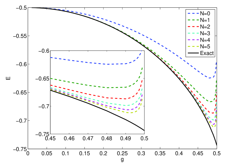
Figure 3: (Color online) Comparison of the ground state energies as function of $g$ calculated by the $N$-th order approximation with the exact results at $\Omega=1$.

5 Variational calculation for the ground state

The ground state corresponds to $q=\frac{1}{4}$ and negative parity, so we have

$$\beta\left(2m-v^{2}\right)u_{m}^{(q)}-\sum_{n=0}^{N_{\mathrm{tr}}}u_{n}^{(q)}\ D_{m,n}^{(q)}=Eu_{m}^{(q)},$$ (31)

where $N_{\mathrm{tr}}$ is truncation number. The lowest energy obtained from the above eigenvalue problem will give the ground-state energy $E_{\mathrm{GS}}^{(N_{\mathrm{tr}})}$ in the $N_{\mathrm{tr}}$-th order of approximation. $E_{\mathrm{GS}}^{(1)}$corresponds to $N_{\mathrm{tr}}=1$.

We plot the GS energy as a function of coupling strength in different order of approximations for $\Omega=1$, in figure 3. The GS energy becomes closer to the exact one as the approximation order increases, but it tends to the collapse value $-\frac{1}{2}$ finally as $g$ goes to $\frac{1}{2}$ in any finite order approximation. This holds as well for all states below the continuum discussed in section  3. It indicates that any finite order approximation misses the low energy features of the spectrum at the critical coupling.

We elucidate this finding by performing a variational study for the ground-state with negative parity. The trial wavefunction reads for $\Pi=-1,q=\frac{1}{4}$

$$\left|{GS_{trial}}\right\rangle_{q=\frac{1}{4}}\varpropto\left(\ \begin{array}[]{l}\left|\frac{1}{4},0\right\rangle_{b^{\prime}}\\ \left|\frac{1}{4},0\right\rangle_{c^{\prime}}\end{array}\right),$$ (32)

with

$$b=u^{\prime}a+v^{\prime}a^{\dagger},\qquad c=u^{\prime}a-v^{\prime}a^{\dagger},$$ (33)

where

$$u^{\prime}=\cosh r,\qquad v^{\prime}=\sinh r,$$ (34)

and the variational parameter $r$. The corresponding energy reads then

$$E(r)=-\frac{\Omega}{2}\left[1-\tanh^{2}\left(2r\right)\right]^{1/4}+\omega\sinh^{2}\left(r\right)-g\sinh\left(2r\right).$$ (35)

Minimizing $E(r)$ with respect to $r$ gives a variational estimate for the ground-state energy.

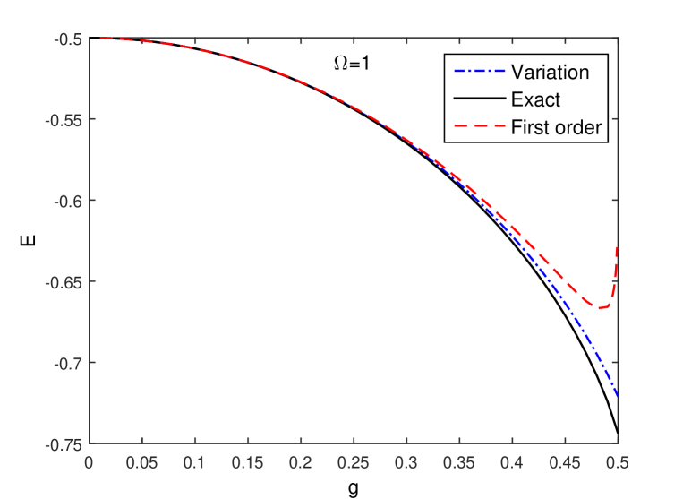
Figure 4: (Color online) Comparison of the ground state energies as function of $g$ calculated by the variational ansatz, the first order approximation and the exact results at $\Omega=1$.

In figure 4, we compare the GS energies obtained by the above variational ansatz with those of the first-order approximation and the exact G-function technique. It is found that the variational GS energy is much better than obtained in the first-order approximation. More interestingly, the variational GS energy does not collapse towards $-\frac{1}{2}$. This proves that the lower edge of the continuum cannot coincide with the groundstate of the system which is always gapped.

6 Conclusions

In this work, we have derived the $G$-function for the two-photon QRM in a concise and compact way, by using extended squeezed states for each Bargmann index. Zeros of the $G$-function determine the regular spectrum. The average distance between energy levels is dictated by the pole structure of $G(E)$. If the $n$-th level for any finite $n$ is located between two poles as $g$ tends to $\frac{1}{2}$, this level will collapse to the value $-\frac{1}{2}$ at $g=\frac{1}{2}$. The ground state is located below the first pole for $g\ll 1$ and remains so until $g_{\mathrm{c}}$ is reached. However, a crossing of the zeroth baseline from below cannot be ruled out, because non-degenerate exceptional solutions are possible for $n=0$. It seems that these always belong to excited states with positive parity and large $\Omega$: the zeroth baseline is crossed from above so that this state lies in the gap between ground state and continuum at $g=g_{\mathrm{c}}$. In general the $G$-function has several zeros below $E=-\frac{1}{2}$ for large $\Omega$ and small $g$. All of them seem to remain separated from the continuum at the collapse point. We have calculated explicit solutions in a finite-dimensional approximation scheme and found that the zeroth order describes the collapse well but the gap and the discrete levels inside do not appear in any finite order approximation. Nevertheless, the existence of the gap itself can be proven by a simple variational analysis of the ground state.

References

References

- [1] Rabi I I 1936 Phys. Rev. 49 324 Rabi I I 1937 Phys. Rev. 51 652
- [2] Jaynes E T and Cummings F W 1963 Proc. IEEE 51 89
- [3] Scully M O and Zubairy M S 1997 Quantum Optics (Cambridge University Press, Cambridge) Orszag M 2007 Quantum Optics Including Noise Reduction, Trapped Ions, Quantum Trajectories, and Decoherence (Science Publishing Group, New York)
- [4] Bargmann V 1961 Comm. Pure Appl. Math. 14 197
- [5] Braak D 2011 Phys. Rev. Lett. 107 100401
- [6] Slavyanov S Y and Lay W 2000 Special Functions: A Unified Theory Based on Singularities (Oxford University Press, New York)
- [7] Chen Q H, Wang C, He S, Liu T, and Wang K L 2012 Phys. Rev. A 86 023822
- [8] Travenec I 2012 Phys. Rev. A 85 043805
- [9] Moroz A 2012 Europhys. Lett. 100 60010
- [10] Gardas B and Dajka J 2013 \jpa46 265302
- [11] Braak D 2013 J. Phys. B: At. Mol. Opt. Phys.46 224007
- [12] Chilingaryan S A and Rodríguez-Lara B M 2013 \jpa46 335301
- [13] Maciejewski A J, Przybylska M and Stachowiak T 2014 Phys. Lett. A 378 3445
- [14] Zhong H, Xie Q, Batchelor M T and Lee C 2013 \jpa46 415302 Zhong H, Xie Q, Guan X, Batchelor M T, Gao K and Lee C 2014 \jpa47 045301
- [15] Wang H, He S, Duan L and Chen Q H 2014 EPL 106 54001 Duan L, He S and Chen Q H 2015 Ann. Phys., NY355 121
- [16] Xie Q T, Cui S, Cao J P, Amico L and Fan H 2014 Phys. Rev. X 4 021046
- [17] Tomka M, Araby O E, Pletyukhov M and Gritsev V 2014 Phys. Rev. A90 063839
- [18] Peng J, Ren Z, Braak D, Guo G, Ju G, Zhang X and Guo X 2014 \jpa47 265303 Peng J, Ren Z, Yang H, Guo G, Zhang X, Ju G, Guo X, Deng C and Hao G 2015 \jpa48, 285301
- [19] He S, Duan L and Chen Q H 2015 New J. Phys. 17, 043033
- [20] Batchelor M T and Zhou H Q 2015 Phys. Rev. A 91053808
- [21] Bertet P, Osnaghi S, Milman P, Auffeves A, Maioli P, Brune M, Raimond J M and Haroche S 2002 Phys. Rev. Lett. 88 143601
- [22] Brune M, Raimond J M, Goy P, Davidovich L and Haroche S 1987 Phys. Rev. Lett. 59 1899
- [23] Stufler S, Machnikowski P, Ester P, Bichler M, Axt V M, Kuhn T and Zrenner A 2006 Phys. Rev. B 73 125304
- [24] Valle E D, Zippilli S, Laussy F P, Gonzalez-Tudela A, Morigi G and Tejedor C 2010 Phys. Rev. B 81 035302 Ota Y, Iwamoto S, Kumagai N and Arakawa Y 2011 Phys. Rev. Lett. 107 233602
- [25] Puri R R and Bullough R K 1988 J. Opt. Soc. Am. B 5 2021 Dung H T and Huyen N D 1994 Phys. Rev. A 49 473
- [26] Toor A H and Zubairy M S 1992 Phys. Rev. A 45 4951 Peng J S and Li G X 1993 Phys. Rev. A 47 3167 Ng K M, Lo C F and Liu K L 1999 Eur. Phys. J. D 6 119 Emary C and Bishop R F 2002 J. Math. Phys. (NY) 43 3916 Dolya S N 2009 J. Math. Phys. 50 033512
- [27] Albert V V, Scholes G D and Brumer P 2011 Phys. Rev. A 84 042110
- [28] Zhang Y Z 2013 J. Math. Phys. 54 102104 Zhang Y Z 2014 Analytic solutions of 2-photon and two-mode Rabi models arXiv: 1304.7827v2 Zhang Y Z 2015 On the -mode and -photon quantum Rabi models arXiv: 1507.03863v1
- [29] Felicetti S, Pedernales J S, Egusquiza I L, Romero G, Lamata L, Braak D and Solano E 2015 Phys. Rev. A 92 033817
- [30] Casanova J, Romero G, Lizuain I, García-Ripoll J J and Solano E 2010 Phys. Rev. Lett. 105 263603
- [31] Wang Y K and Hioe F T 1973 Phys. Rev. A 7 831
- [32] Duan L, He S, Braak D and Chen Q H 2015 EPL 112 34003
- [33] Maciejewski A J, Przybylska M and Stachowiak T 2014 Phys. Lett. A 378 16
- [34] Braak D 2015 Proceedings of the Forum “Math-for-Industry 2014” Springer