Gain Function Approximation in the Feedback Particle Filter

Abstract

This paper is concerned with numerical algorithms for gain function approximation in the feedback particle filter. The exact gain function is the solution of a Poisson equation involving a probability-weighted Laplacian. The problem is to approximate this solution using only particles sampled from the probability distribution. Two algorithms are presented: a Galerkin algorithm and a kernel-based algorithm. Both the algorithms are adapted to the samples and do not require approximation of the probability distribution as an intermediate step. The paper contains error analysis for the algorithms as well as some comparative numerical results for a non-Gaussian distribution. These algorithms are also applied and illustrated for a simple nonlinear filtering example.

I Introduction

This paper is concerned with algorithms for numerically approximating the solution of a certain linear partial differential equation (pde) that arises in the problem of nonlinear filtering. In continuous time, the filtering problem pertains to the following stochastic differential equations (sdes):

$$\,\mathrm{d}X_{t} =a(X_{t})\,\mathrm{d}t+\,\mathrm{d}B_{t},$$ (1a)

$$\,\mathrm{d}Z_{t} =h(X_{t})\,\mathrm{d}t+\,\mathrm{d}W_{t},$$ (1b)

where $X_{t}\in\mathbb{R}^{d}$ is the (hidden) state at time $t$, $Z_{t}\in\mathbb{R}$ is the observation, and $\{B_{t}\}$, $\{W_{t}\}$ are two mutually independent standard Wiener processes taking values in $\mathbb{R}^{d}$ and $\mathbb{R}$, respectively. The mappings $a(\cdot):\mathbb{R}^{d}\rightarrow\mathbb{R}^{d}$ and $h(\cdot):\mathbb{R}^{d}\rightarrow\mathbb{R}$ are $C^{1}$ functions. Unless noted otherwise, all probability distributions are assumed to be absolutely continuous with respect to the Lebesgue measure, and therefore will be identified with their densities. The choice of observation being scalar-valued ($Z_{t}\in\mathbb{R}$) is made for notational ease.

The objective of the filtering problem is to estimate the posterior distribution of $X_{t}$ given the time history of observations (filtration) ${\cal Z}_{t}:=\sigma(Z_{s}:0\leq s\leq t)$. The density of the posterior distribution is denoted by $p^{*}$, so that for any measurable set $A\subset\mathbb{R}^{d}$,

$$\int_{x\in A}p^{*}(x,t)\,\,\mathrm{d}x={\sf P}[X_{t}\in A\mid{\cal Z}_{t}].$$

The filter is infinite-dimensional since it defines the evolution, in the space of probability measures, of $\{p^{*}(\,\cdot\,,t):t\geq 0\}$. If $a(\,\cdot\,)$, $h(\,\cdot\,)$ are linear functions, the solution is given by the finite-dimensional Kalman-Bucy filter. The article [3] surveys numerical methods to approximate the nonlinear filter. One approach described in this survey is particle filtering.

The particle filter is a simulation-based algorithm to approximate the filtering task [14]. The key step is the construction of $N$ stochastic processes $\{X^{i}_{t}:1\leq i\leq N\}$: The value $X^{i}_{t}\in\mathbb{R}^{d}$ is the state for the $i$-th particle at time $t$. For each time $t$, the empirical distribution formed by the particle population is used to approximate the posterior distribution. Recall that this is defined for any measurable set $A\subset\mathbb{R}^{d}$ by,

$$p^{(N)}(A,t)=\frac{1}{N}\sum_{i=1}^{N}\text{\rm\large 1}[X^{i}_{t}\in A].$$

A common approach in particle filtering is called sequential importance sampling, where particles are generated according to their importance weight at every time step [1, 14].

In our earlier papers [17, 16, 18], an alternative feedback control-based approach to the construction of a particle filter was introduced. The resulting particle filter, referred to as the feedback particle filter (FPF), is a controlled system. The dynamics of the $i$-th particle have the following gain feedback form,

$$\,\mathrm{d}X^{i}_{t}=a(X^{i}_{t})\,\mathrm{d}t+\,\mathrm{d}B^{i}_{t}+{\sf K}_{t}(X^{i}_{t})\circ(\,\mathrm{d}Z_{t}-\frac{h(X^{i}_{t})+\hat{h}_{t}}{2}\,\mathrm{d}t),$$ (2)

where $\{B^{i}_{t}\}$ are mutually independent standard Wiener processes and $\hat{h}_{t}:={\sf E}[h(X_{t}^{i})|\mathcal{Z}_{t}]$. The initial condition $X^{i}_{0}$ is drawn from the initial density $p^{*}(x,0)$ of $X_{0}$ independent of $\{B^{i}_{t}\}$. Both $\{B^{i}_{t}\}$ and $\{X^{i}_{0}\}$ are also assumed to be independent of $X_{t},Z_{t}$. The $\circ$ indicates that the sde is expressed in its Stratonovich form.

The gain function ${\sf K}_{t}$ is obtained by solving a weighted Poisson equation: For each fixed time $t$, the function $\phi$ is the solution to a Poisson equation,

BVP $$\begin{aligned} \nabla\cdot(p(x,t)\nabla\phi(x,t))&=-(h(x)-\hat{h})p(x,t),\\ \int\phi(x,t)p(x,t)\,\mathrm{d}x&=0\qquad\text{(zero-mean)},\end{aligned}$$ (3)

for all $x\in\mathbb{R}^{d}$ where $\nabla$ and $\nabla\cdot$ denote the gradient and the divergence operators, respectively, and $p$ denotes the conditional density of $X_{t}^{i}$ given $\mathcal{Z}_{t}$.

In terms of the solution $\phi$, the gain function is given by,

$${\sf K}_{t}(x)=\nabla\phi(x,t)\,.$$

Note that the gain function ${\sf K}_{t}$ is vector-valued (with dimension $d\times 1$) and it needs to be obtained for each fixed time $t$. For the linear Gaussian case, the gain function is the Kalman gain. For the general nonlinear non-Gaussian problem, the FPF (2) is exact, given an exact gain function and an exact initialization $p(\,\cdot\,,0)=p^{*}(\,\cdot\,,0)$. Consequently, if the initial conditions $\{X^{i}_{0}\}_{i=1}^{N}$ are drawn from the initial density $p^{*}(\,\cdot\,,0)$ of $X_{0}$, then, as $N\rightarrow\infty$, the empirical distribution of the particle system approximates the posterior density $p^{*}(\,\cdot\,,t)$ for each $t$.

A numerical implementation of the FPF (2) requires a numerical approximation of the gain function ${\sf K}_{t}$ and the mean $\hat{h}_{t}$ at each time-step. The mean is approximated empirically, $\hat{h}_{t}\approx\frac{1}{N}\sum_{i=1}^{N}h(X_{t}^{i})=:\hat{h}_{t}^{(N)}$. The gain function approximation - the focus of this paper - is a challenging problem because of two reasons: i) Apart from the linear Gaussian case, there are no known closed-form solutions of (3); ii) The density $p(x,t)$ is not explicitly known. At each time-step, one only has samples $X^{i}_{t}$. These are assumed to be i.i.d sampled from $p$. Apart from the FPF algorithm, solution of the Poisson equation is also central to a number of other algorithms for nonlinear filtering [5, 15].

In our prior work, we have obtained results on existence, uniqueness and regularity of the solution to the Poisson equation, based on certain weak formulation of the Poisson equation. The weak formulation led to a Galerkin numerical algorithm. The main limitation of the Galerkin is that the algorithm requires a pre-defined set of basis functions - which scales poorly with the dimension $d$ of the state. The Galerkin algorithm can also exhibit certain numerical issues related to the Gibb’s phenomena. This can in turn lead to numerical instabilities in simulating the FPF.

The contributions of this paper are as follows: We present a new basis-free kernel-based algorithm for approximating the solution of the gain function. The key step is to construct a Markov matrix on a certain graph defined on the space of particles $\{X^{i}_{t}\}_{i=1}^{N}$. The value of the function $\phi$ for the particles, $\phi(X^{i}_{t})$, is then approximated by solving a fixed-point problem involving the Markov matrix. The fixed-point problem is shown to be a contraction and the method of successive approximation applies to numerically obtain the solution.

We present results on error analysis for both the Galerkin and the kernel-based method. These results are illustrated with the aid of an example involving a multi-modal distribution. Finally, the two methods are compared for a filtering problem with a non-Gaussian distribution.

In the remainder of this paper, we express the linear operator in (3) as a weighted Laplacian $\Delta_{\rho}\phi:=\frac{1}{\rho}\nabla\cdot(\rho\nabla\phi)$ where additional assumptions on the density $\rho$ appear in the main body of the paper. In recent years, this operator and the associated Markov semigroup have received considerable attention with several applications including spectral clustering, dimensionality reduction, supervised learning etc [4, 10]. For a mathematical treatment, see the monographs [8, 2]. Related specifically to control theory, there are important connections with stochastic stability of Markov operators [7, 13].

The outline of this paper is as follows: The mathematical preliminaries appear in Sec. II. The Galerkin and the kernel-based algorithms for the gain function approximation appear in Sec. III and Sec. IV, respectively. The nonlinear filtering example appears in Sec. V.

II Mathematical Preliminaries

The Poisson equation (3) is expressed as,

BVP $$\begin{aligned} -\Delta_{\rho}\phi&=h,\\ \int\phi\rho\,\mathrm{d}x&=0\qquad\text{(zero-mean)},\end{aligned}$$ (4)

where $\rho$ is a probability density on $\mathbb{R}^{d}$, $\Delta_{\rho}\phi:=\frac{1}{\rho}\nabla\cdot(\rho\nabla\phi)$ and, without loss of generality, it is assumed $\hat{h}=\int h\rho\,\mathrm{d}x=0$.

Problem statement: Approximate the solution $\phi(X^{i})$ and $\nabla\phi(X^{i})$ given $N$ independent samples $X^{i}$ drawn from $\rho$. The density $\rho$ is not explicitly known.

For the problem to be well-posed requires definition of the function spaces and additional assumptions on $\rho$ and $h$ enumerated next: Throughout this paper, $\mu$ is an absolutely continuous probability measure on $\mathbb{R}^{n}$ with associated density $\rho$. $L^{2}(\mathbb{R}^{d},\mu)$ is the Hilbert space of square integrable functions on $\mathbb{R}^{d}$ equipped with the inner-product,

$$<\phi,\psi>:=\int\phi(x)\psi(x)\,\mathrm{d}\mu(x).$$

The associated norm is denoted as $\|\phi\|^{2}_{2}:=<\phi,\phi>$. The space $H^{1}(\mathbb{R}^{d},\mu)$ is the space of square integrable functions whose derivative (defined in the weak sense) is in $L^{2}(\mathbb{R}^{d},\mu)$. We use $L^{2}$ and $H^{1}$ to denote $L^{2}(\mathbb{R}^{d},\mu)$ and $H^{1}(\mathbb{R}^{d},\mu)$, respectively. For the zero-mean solution of interest, we additionally define the co-dimension 1 subspace $L^{2}_{0}:=\{\phi\in L^{2};\int\phi\,\mathrm{d}\mu=0\}$ and $H^{1}_{0}:=\{\phi\in H^{1};\int\phi\,\mathrm{d}\mu=0\}$. $L^{\infty}$ is used to denote the space of functions that are bounded a.e. (Lebesgue) and the sup-norm of a function $\phi\in L^{\infty}$ is denoted as $\|\phi\|_{\infty}$.

The following assumptions are made throughout the paper:

• Assumption A1: The probability density function $\rho$ is of the form $\rho(x)=e^{-(x-\mu)^{T}\Sigma^{-1}(x-\mu)-V(x)}$ where $\mu\in\mathbb{R}^{d}$, $\Sigma$ is a positive-definite matrix and $V\in C^{2}$ with $V\in L^{\infty}$, and its derivatives $DV,D^{2}V\in L^{\infty}$.

• Assumption A2: The function $h\in L^{2}$ and $\int h\,\mathrm{d}\mu=0$.

Under assumption A1, the density $\rho$ admits a spectral gap (or Poincaré inequality)[2], i.e $\exists\;\lambda_{1}>0$ such that,

$$\int\phi^{2}\rho\,\mathrm{d}x\leq\frac{1}{\lambda_{1}}\int|\nabla\phi|^{2}\rho\,\mathrm{d}x,\quad\forall\phi\in H^{1}_{0}.$$ (5)

Furthermore, the spectrum is known to be discrete with an ordered sequence of eigenvalues $0=\lambda_{0}<\lambda_{1}\leq\lambda_{2}\leq\ldots$ and associated eigenfunctions $\{e_{n}\}$ that form a complete orthonormal basis of $L^{2}$ [Corollary 4.10.9 in  [2]]. The trivial eigenvalue $\lambda_{0}=1$ with associated eigenfunction $e_{0}=1$. On the subspace of zero-mean functions, the spectral decomposition yields: For $\phi\in L^{2}_{0}$,

$$-\Delta_{\rho}\phi=\sum_{m=1}^{\infty}\lambda_{m}<e_{m},\phi>e_{m}.$$ (6)

The spectral gap condition (5) implies that $\lambda_{1}>0$. Consequently, the semigroup

$$e^{t\Delta_{\rho}}\phi:=\sum_{m=1}^{\infty}e^{-t\lambda_{m}}<e_{m},\phi>e_{m}$$ (7)

is a strict contraction on the subspace $L^{2}_{0}$. It is also easy to see that $\mu$ is an invariant measure and $\int e^{t\Delta_{\rho}}\phi(x)\,\mathrm{d}\mu(x)=\int\phi(x)\,\mathrm{d}\mu(x)=0$ for all $\phi\in L^{2}_{0}$.

Example 1

If the density $\rho$ is Gaussian with mean $\mu\in\mathbb{R}^{d}$ and a positive-definite covariance matrix $\Sigma$, the spectral gap constant (1/$\lambda_{1}$) equals the largest eigenvalue of $\Sigma$. The eigenfunctions are the Hermite functions. Given a linear function $h(x)=H\cdot x$, the unique solution of the BVP (4) is given by,

$$\phi(x)=(\Sigma H)\cdot(x-\mu),$$

where $\cdot$ denotes the vector dot product in $\mathbb{R}^{d}$. In this case, ${\sf K}=\nabla\phi=\Sigma H$ is the Kalman gain.  

Example 2

In the scalar case (where $d=1$), the Poisson equation is:

$$-\frac{1}{\rho(x)}\frac{\,\mathrm{d}}{\,\mathrm{d}x}(\rho(x)\frac{\,\mathrm{d}\phi}{\,\mathrm{d}x}(x))=h.$$

Integrating twice yields the solution explicitly,

$$\frac{\,\mathrm{d}\phi}{\,\mathrm{d}x}(x) =-\frac{1}{\rho(x)}\int_{-\infty}^{x}\rho(z)h(z)\,\mathrm{d}z$$ (8)

$$\phi(x) =-\int_{-\infty}^{x}\frac{\,\mathrm{d}y}{\rho(y)}\int_{-\infty}^{y}\rho(z)h(z)\,\mathrm{d}z$$

For the particular choice of $\rho$ as the sum of two Gaussians $N(-1,\sigma^{2})$ and $N(+1,\sigma^{2})$ with $\sigma=0.4$ and $h(x)=x$, the solution obtained using (8) is depicted in Fig. 1. Since $\frac{\,\mathrm{d}h}{\,\mathrm{d}x}>0$, the positivity of the gain function $\frac{\,\mathrm{d}\phi}{\,\mathrm{d}x}(x)$ follows from the maximum principle for elliptic pdes [6].  

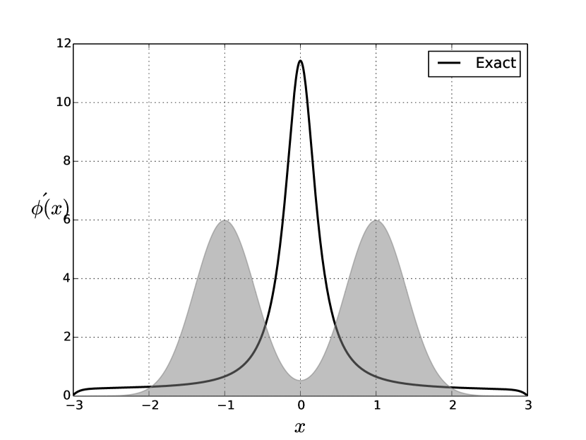
Figure 1: The exact solution to the Poisson equation using the formula (8). The density $\rho$ is the sum of two Gaussians $N(-1,\sigma^{2})$ and $N(+1,\sigma^{2})$, and $h(x)=x$. The density is depicted as the shaded curve in the background.

III Galerkin for Gain Function Approximation

Weak formulation: A function $\phi\in H_{0}^{1}$ is said to be a weak solution of Poisson’s equation (4) if

$$<\nabla\phi,\nabla\psi>=<h,\psi>,\quad\forall\;\psi\in H_{0}^{1}.$$ (9)

It is shown in [12] that, under Assumptions (A1)-(A2), there exists a unique weak solution of the Poisson equation.

The Galerkin approximation involves solving (9) in a finite-dimensional subspace $S\subset H^{1}_{0}(\mathbb{R}^{d};\rho)$. The solution $\phi$ is approximated as,

$$\phi^{(M)}(x)=\sum_{m=1}^{M}c_{m}\psi_{m}(x),$$ (10)

where $\{\psi_{m}(x)\}_{m=1}^{M}$ are a given set of basis functions.

The finite-dimensional approximation of (9) is to choose constants $\{c_{m}\}_{m=1}^{M}$ such that

$$<\nabla\phi^{(M)},\nabla\psi>=<h,\psi>,\;\;\forall\;\psi\in S,$$ (11)

where $S:=\text{span}\{\psi_{1},\ldots,\psi_{M}\}\subset H^{1}_{0}$.

Denoting $[A]_{ml}=<\nabla\psi_{l}\cdot\nabla\psi_{m}>$, $b_{m}=<h,\psi_{m}>$, and $c=(c_{1},c_{2},\ldots,c_{M})^{T}$, the finite-dimensional approximation (11) is expressed as a linear matrix equation:

$$Ac=b.$$ (12)

In a numerical implementation, the matrix $A$ and vector $b$ are approximated as,

$$[A]_{ml} =<\nabla\psi_{l}\cdot\nabla\psi_{m}>\approx\frac{1}{N}\sum_{i=1}^{N}\nabla\psi_{l}(X^{i})\cdot\nabla\psi_{m}(X^{i})=:[A]_{ml}^{(N)},$$ (13)

$$b_{m} =<h,\psi_{m}>\approx\frac{1}{N}\sum_{i=1}^{N}h(X^{i})\psi_{m}(X^{i})=:b_{m}^{(N)}.$$ (14)

The resulting solution of the matrix equation (12), with $A=A^{(N)}$ and $b=b^{(N)}$, is denoted as $c^{(N)}$,

$$A^{(N)}c^{(N)}=b^{(N)}.$$ (15)

Using (10), we obtain the particle-based approximation of the solution:

$$\phi^{(M,N)}(x)=\sum_{m=1}^{M}c_{m}^{(N)}\psi_{m}(x).$$ (16)

In terms of this solution, the gain function is obtained as,

$$\nabla\phi^{M,N}(x)=\sum_{m=1}^{M}c_{m}^{(N)}\nabla\psi_{m}(x).$$

Convergence analysis: The following is a summary of the approximations in the Galerkin algorithm:

$$\text{Exact}: <\nabla\phi,\nabla\psi> =<h,\psi>,\quad\forall\psi\in H_{0}^{1}$$

Galerkin approx: $$<\nabla\phi^{(M)},\nabla\psi> =<h,\psi>,\;\forall\psi\in S\subset H_{0}^{1}$$

Empirical approximation:

$$\frac{1}{N}\sum_{i=1}^{N}\nabla\phi^{(M,N)}(X^{i})\cdot\nabla\psi(X^{i})=\frac{1}{N}\sum_{i=1}^{N}h(X^{i})\psi(X^{i}),\;\;\forall\psi\in S$$

We are interested in the error analysis of these approximations as a function of both $M$ and $N$. Note that the approximation error $\phi^{(M)}-\phi^{(M,N)}$ is random because $X^{i}$ are sampled randomly from the probability distribution $\mu$. The following Proposition provides error bounds for the case where the basis functions are the eigenfunctions of the Laplacian. The proof appears in the Appendix -A.

Proposition 1

Consider the empirical Galerkin approximation of the Poisson equation (9) on the space $S:=\text{span}\{e_{1},e_{2},\ldots,e_{M}\}$ of the first $M$ eigenfunctions. Fix $M<\infty$. Then the solution for the matrix equation (15) exists with probability approaching 1 as $N\rightarrow\infty$. And there is a sequence of random variables $\{\epsilon_{N}\}$ such that

$$\|\phi^{(M,N)}-\phi\|_{2}\leq\frac{1}{\lambda_{M}^{2}}\|h\|^{2}_{2}+\epsilon_{N},$$ (17)

where $\epsilon_{N}\rightarrow 0$ as $N\rightarrow\infty$ a.s.  

Remark 1

In practice, the eigenfunctions of the Laplacian are not known. The basis functions are typically picked from the polynomial family, e.g., the Hermite functions. In this case, the bounds will provide qualitative assessment of the error provided the eigenfunctions associated with the first $M$ eigenvalues are ‘approximately’ in $S$. Quantitatively, the additional error may be bounded in terms of the projection error between the eigenfunction and the projection onto $S$.  

Example 3

We next revisit the bimodal distribution first introduced in the Example 1. Fig. 2 depicts the empirical Galerkin approximation, with $N=200$ samples, of the gain function. The basis functions are from the polynomial family - $\{x,x^{2},\ldots,x^{M}\}$ - and the figure depicts the gain functions with $M=1,3,5$ modes. The $(M=1)$ case is referred to as the constant-gain approximation where,

$$\frac{\,\mathrm{d}\phi}{\,\mathrm{d}x}(x)=\int h(x)\,x\;\,\mathrm{d}\mu(x)=(\text{const.})$$

For the linear Gaussian case, the (const.) is the Kalman gain. The plots included in the Figure demonstrate the Gibb’s phenomena as more and more modes are included in the Galerkin. Particularly concerning is the change in the sign of the gain which leads to negative values of gain for some particles contradicting the positivity property of the gain described in Example 1. As discussed in the filtering example in Sec. V, the negative values of the gain can cause numerical issues and lead to erroneous results for the filter.  

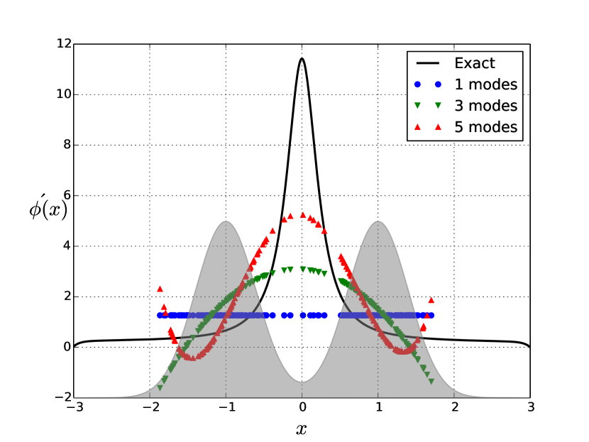
Figure 2: Comparison of the exact solution and its empirical Galerkin approximation with $M=1,3,5$ modes and $N=200$ particles. The density is depicted as the shaded curve in the background.

IV Semigroup Approximation of the Gain

Semigroup formulation: The semigroup formula (7) is used to construct the solution of the Poisson equation by solving the following fixed-point equation for any fixed positive value of $t$:

$$\phi=e^{t\Delta_{\rho}}\phi+\int_{0}^{t}e^{s\Delta_{\rho}}h\,\mathrm{d}s.$$ (18)

A unique solution exists because $e^{t\Delta_{\rho}}$ is a contraction on $L^{2}_{0}$.

The approximation proposed in this section involves approximating the semigroup as a perturbed integral operator, for small positive values of $t=\epsilon$. The following approximation of the semigroup appears in [4, 10]:

$${T}^{(\epsilon)}\phi(x):=\frac{\int{k}^{(\epsilon)}(x,y)\phi(y)\,\mathrm{d}\mu(y)}{\int{k}^{(\epsilon)}(x,y)\,\mathrm{d}\mu(y)},$$ (19)

where ${k}^{(\epsilon)}(x,y):=\frac{{g}^{(\epsilon)}(x,y)}{\sqrt{\int{g}^{(\epsilon)}(x,y)\,\mathrm{d}\mu(y)}\sqrt{\int{g}^{(\epsilon)}(x,y)\,\mathrm{d}\mu(x)}}$ and ${g}^{(\epsilon)}(x,y):=\frac{1}{(4\pi\epsilon)^{\frac{d}{2}}}\exp{(-\frac{|x-y|^{2}}{4\epsilon})}$ is the Gaussian kernel in $\mathbb{R}^{d}$.

In terms of the perturbed integral operator, the fixed-point equation (18) becomes,

$${\phi}^{(\epsilon)}={T}^{(\epsilon)}{\phi}^{(\epsilon)}+\int_{0}^{\epsilon}T^{(s)}h\,\mathrm{d}s.$$ (20)

The superscript $\epsilon$ is used to distinguish the approximate ($\epsilon$-dependent) solution from the exact solution $\phi$. As shown in the Appendix -B, ${T}^{(\epsilon)}$ has an ergodic invariant measure ${\mu}^{(\epsilon)}$ which approximates $\mu$ as $\epsilon\downarrow 0$. For any fixed positive $\epsilon$, we are interested in solutions that are zero-mean with respect to this measure. The existence-uniqueness result for this solution is described next; the proof appears in the Appendix -B.

Proposition 2

Consider the fixed-point problem (20) with the perturbed operator ${T}^{(\epsilon)}$ defined according to (19). Fix $\epsilon>0$. Then there exists a unique solution ${\phi}^{(\epsilon)}$ such that $\int{\phi}^{(\epsilon)}\,\mathrm{d}{\mu}^{(\epsilon)}=0$.  

In a numerical implementation, the solution $\phi^{\epsilon}$ is approximated directly for the particles:

$$\Phi^{(\epsilon,N)} :=({\phi}^{(\epsilon)}(X^{1}),{\phi}^{(\epsilon)}(X^{2}),\cdots,{\phi}^{(\epsilon)}(X^{N})).$$

The integral operator ${T}^{(\epsilon)}$ is approximated as a $N\times N$ Markov matrix whose $(i,j)$ entry is obtained empirically as,

$${T}^{(\epsilon,N)}_{i,j}=\frac{{k}^{(\epsilon,N)}(X^{i},X^{j})}{\sum_{l=1}^{N}{k}^{(\epsilon,N)}(X^{i},X^{l})},$$ (21)

where ${k}^{(\epsilon,N)}(x,y)=\frac{g^{\epsilon}(x,y)}{\sqrt{\frac{1}{N}\sum_{l=1}^{N}g^{\epsilon}(x,X^{l})}\sqrt{\frac{1}{N}\sum_{l=1}^{N}g^{\epsilon}(y,X^{l})}}$.

The resulting finite-dimensional fixed-point equation is given by,

$$\Phi^{(\epsilon,N)}={T}^{(\epsilon,N)}\Phi^{(\epsilon,N)}+\int_{0}^{\epsilon}T^{(s,N)}H^{(N)}\,\mathrm{d}s,$$ (22)

where $\Phi^{(\epsilon,N)}=(\Phi^{(\epsilon,N)}_{1},\Phi^{(\epsilon,N)}_{2},\ldots,\Phi^{(\epsilon,N)}_{N})\in\mathbb{R}^{N}$ is the vector-valued solution, $H^{(N)}=(h(X^{1}),h(X^{2}),\cdots,h(X^{N}))\in\mathbb{R}^{N}$, and ${T}^{(\epsilon,N)}$ and $T^{(s,N)}$ are $N\times N$ matrices defined according to (21). The existence-uniqueness result for the zero-mean solution of the finite-dimensional equation (22) is described next; its proof is given in the Appendix -C. The zero-mean property is the finite-dimensional counterpart of the zero-mean condition $\int\phi\,\mathrm{d}\mu=0$ for the original problem and $\int\phi\,\mathrm{d}\mu^{\epsilon}=0$ for the perturbed problem.

Proposition 3

Consider the fixed-point problem (22) with the matrix ${T}^{(\epsilon,N)}$ defined according to (21). Then, with probability $1$, there exists a unique zero-mean solution $\Phi^{(\epsilon,N)}\in\mathbb{R}^{d}$.  

Once $\Phi^{(\epsilon,N)}$ is available, it is straightforward to extend it to the entire domain. For $x\in\mathbb{R}^{d}$,

$${\phi}^{(\epsilon,N)}(x):=\frac{\sum_{i=1}^{N}{k}^{(\epsilon,N)}(x,X^{i})\Phi^{(\epsilon,N)}_{i}}{\sum_{i=1}^{N}{k}^{(\epsilon,N)}(x,X^{i})}+\int_{0}^{\epsilon}T^{(s,N)}h(x)\,\mathrm{d}s.$$ (23)

By construction ${\phi}^{(\epsilon,N)}(X^{i})=\Phi^{(\epsilon,N)}_{i}$ for $i=1,\ldots,N$. The extension is not necessary for filtering because one only needs to solve for $\nabla\phi$ at $X^{i}$. The formula for this is,

$$\frac{\partial\phi}{\partial x_{l}}(X^{i})=\sum_{j=1}^{N}\left[{T}^{(\epsilon,N)}_{ij}{\Phi}^{(\epsilon,N)}_{j}\left(X^{j}_{l}-\sum_{k=1}^{N}{T}^{(\epsilon,N)}_{ik}X^{k}_{l}\right)\right]$$

where $X^{i}_{l}\in\mathbb{R}$ is the $l$-th component of $X^{i}\in\mathbb{R}^{d}$.

The algorithm is summarized in Algorithm 1. For numerical purposes we use $\epsilon H^{N}\approx\int_{0}^{\epsilon}T^{(s,N)}H^{(N)}\,\mathrm{d}s$. Also, the fixed-point problem (22) is conveniently solved using the method of successive approximation. In filtering, the initial guess is readily available from the solution at the previous time-step.

Algorithm 1 Kernel-based gain function approximation

0:  $\{X^{i}\}_{i=1}^{N}$, $H:=\{h(X^{i})\}_{i=1}^{N}$, $\epsilon$

0:  $\Phi:=\{\phi(X^{i})\}_{i=1}^{N}$, $\{\nabla\phi(X^{i})\}_{i=1}^{N}$

  Calculate $g_{ij}:=\exp(-|X^{i}-X^{j}|^{2}/4\epsilon)$ for $i,j=1$ to $N$.

  Calculate $k_{ij}:=\frac{g_{ij}}{\sqrt{\sum_{l}g_{il}}\sqrt{\sum_{l}g_{jl}}}$ for $i,j=1$ to $N$.

  Calculate $T_{ij}:=\frac{k_{ij}}{\sum_{l}k_{il}}$ for $i,j=1$ to $N$.

  Solve $\Phi=T\Phi+\epsilon H$ for $\Phi$ (Successive approximation).

  Calculate $\frac{\partial\phi}{\partial x_{l}}(X^{i})=\sum_{j=1}^{N}\left[T_{ij}\Phi_{j}\left(X^{j}_{l}-\sum_{k=1}^{N}T_{ik}X^{k}_{l}\right)\right]$ for $l=1$ to $d$.

Convergence: The following is a summary of the approximations with the kernel-based method:

$$\text{Exact}: \phi =e^{\epsilon\Delta_{\rho}}\phi+\int_{0}^{\epsilon}e^{s\Delta_{\rho}}h\,\mathrm{d}s$$

Kernel approx: $${\phi}^{(\epsilon)} ={T}^{(\epsilon)}{\phi}^{(\epsilon)}+\int_{0}^{\epsilon}T^{(s)}h\,\mathrm{d}s$$

Empirical approx: $${\phi}^{(\epsilon,N)} ={T}^{(\epsilon,N)}{\phi}^{(\epsilon,N)}+\int_{0}^{\epsilon}T^{(s,N)}h\,\mathrm{d}s$$

We break the convergence analysis into two steps. The first step involves convergence of ${\phi}^{(\epsilon,N)}$ to ${\phi}^{(\epsilon)}$ as $N\to\infty$. The second step involves convergence of ${\phi}^{(\epsilon)}$ to $\phi$ as $\epsilon\to 0$. The following theorem states the convergence result for the first step; a sketch of the proof appears in Appendix -D.

Theorem 1

Consider the empirical kernel approximation of the fixed-point equation (18). Fix $\epsilon>0$. Then,

• There exists a unique (zero-mean) solution ${\phi}^{(\epsilon)}$ for the perturbed fixed-point equation (20).

• For any finite $N$, a unique (zero-mean) solution $\Phi^{(\epsilon,N)}$ for (22) exists with probability 1.

For a compact set $\Omega\subset\mathbb{R}^{d}$,

$$\lim_{N\to\infty}~{}\sup_{x\in\Omega}|{\phi}^{(\epsilon,N)}(x)-{\phi}^{(\epsilon)}(x)|=0,\quad\text{a.s},$$ (24)

where ${\phi}^{(\epsilon,N)}$ is the extension of the vector-valued solution $\Phi^{(\epsilon,N)}$ (see (23)).  

The convergence analysis for step 2, as $\epsilon\to 0$, is the subject of ongoing work. In this regard, it is shown in [9] that for compactly supported functions $f\in C^{3}$,

$$f(x)-{T}^{(\epsilon)}f(x)=\epsilon\,\Delta_{\rho}f(x)+O(\epsilon^{2}).$$

Example 4

Consider once more the bimodal distribution introduced in 1. Figure 3 depicts the kernel-based approximation of the gain function with $N=200$ particles and range of $\epsilon$. The kernel-based avoids the Gibbs phenomena observed with the Galerkin (see Fig. 2). Notably, the gain function is positive for any choice of $\epsilon$.  

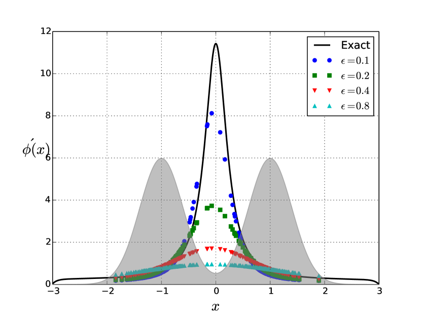
Figure 3: Comparison of the exact solution and its kernel-based approximation with $\epsilon=0.1,0.2,0.4,0.8$ and $N=200$ particles. The density is depicted as the shaded curve in the background.

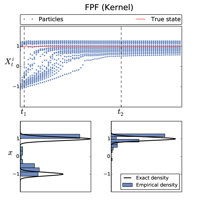
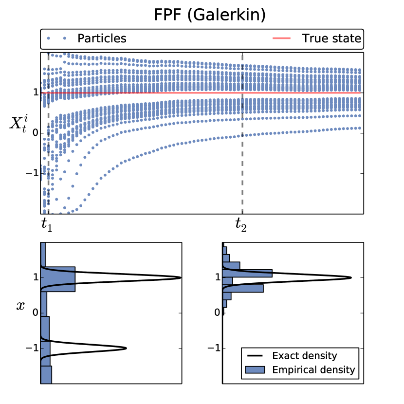
Figure 4: Comparison of simulation results: Trajectory of particles and posterior distribution with (a) Kernel-based approximation of the gain function, (b) Galerkin approximation of the gain function.

V Numerics

In this section, we consider a filtering problem associated with the bimodal distribution introduced in Example 1. The filtering model is given by,

$$\,\mathrm{d}X_{t} =0,$$

$$\,\mathrm{d}Z_{t} =X_{t}\,\mathrm{d}t+\sigma_{w}\,\mathrm{d}W_{t},$$

where $X_{t}\in\mathbb{R}$, $Z_{t}\in\mathbb{R}$, $W_{t}$ is a standard Wiener process, the initial condition $X_{0}$ is sampled from the bimodal distribution comprising of two Gaussians, $N(-1,\sigma^{2})$ and $N(+1,\sigma^{2})$, and without loss of generality, $Z_{0}=0$. As in Example 1, the observation function $h(x)=x$ is linear. The static case is considered because the posterior is given explicitly:

$$p^{*}(x,t)\doteq(\text{const.})\exp\left(\frac{1}{2\sigma_{W}^{2}}h(x)\,Z_{t}-\frac{1}{4\sigma_{W}^{2}}|h(x)|^{2}\,t\right)p_{0}^{*}(x).$$ (25)

The following filtering algorithms are implemented for comparison:

1. Kalman filter;

2. Feedback particle filter with the Galerkin approximation where $S=\text{span}\{x,x^{2},x^{3},x^{4},x^{5}\}$;

3. Feedback particle filter with the kernel approximation.

The performance metrics are as follows:

1. Filter mean $\hat{X}_{t}$;

2. Conditional probability ${\sf P}\left[|X_{t}-X_{0}|<\frac{1}{2}|{\cal Z}_{t}\right]$.

The simulation parameters are as follows: The true initial state $X_{0}=1$. The measurement noise parameter $\sigma_{W}=0.3$. The simulation is carried out over a finite time-horizon $t\in[0,T]$ with $T=0.8$ and a fixed discretized time-step $\Delta t=0.02$. All the particle filters use $N=100$ particles and have the same initialization, where particles are drawn with equal probability from one of the two Gaussians, $N(-1,\sigma^{2})$ or $N(+1,\sigma^{2})$, where $\sigma=0.1$. For the kernel approximation, we use $\epsilon=0.15$. The simulation parameters are tabulated in Table I. The Kalman filter is initialized with $\hat{X}_{0}=0$ and $\Sigma_{0}=\text{Var}(X_{0})=1+\sigma^{2}$. The latter corresponds to the variance of the prior. Figure 4 parts (a) and (b) depict the particle trajectories and the associated distributions obtained using the kernel approximation and the Galerkin approximation, respectively. The kernel-based approximation provides for a better approximation of the exact posterior. At time $t_{1}$ during the initial transients, some of the particles with the Galerkin approximation show a divergence. This is a numerical issue due to the Gibb’s phenomena that leads to erroneous negative value of the gain (see the discussion in Examples 1 and  3).

Figure 5 depicts a comparison of the simulation results for the two metrics. For the particle filters, these are computed empirically.

For applications of FPF with kernel-based approximation of the gain function for attitude estimation problem see the companion paper [19].

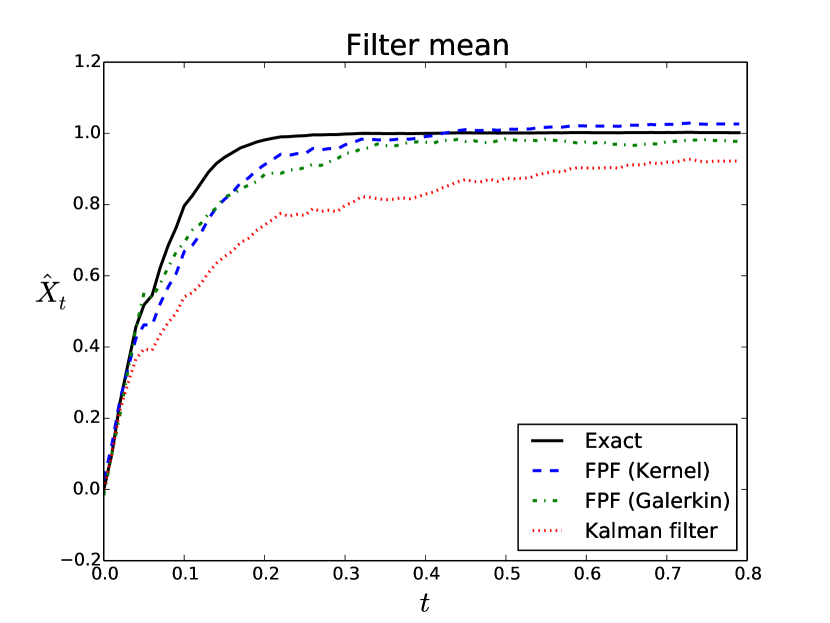
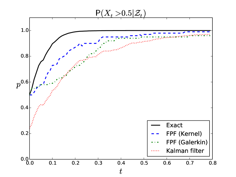
Figure 5: Comparison of simulation results: (a) Conditional mean of the state $X_{t}$, (b) Conditional probability of $X_{t}$ larger than $\frac{1}{2}$.

-A Proof of Proposition 1

Using the spectral representation (6), because $h\in L^{2}$,

$$\phi=-\Delta_{\rho}^{-1}h=\sum_{m=1}^{\infty}\frac{1}{\lambda_{m}}<e_{m},h>e_{m}.$$

With basis functions as eigenfunctions,

$$\phi^{(M)}=\sum_{m=1}^{M}\frac{1}{\lambda_{m}}<e_{m},h>e_{m}.$$

Therefore,

$$\|\phi-\phi^{(M)}\|^{2}_{2}=\sum_{m=M+1}^{\infty}\frac{1}{\lambda_{m}^{2}}|<e_{m},h>|^{2}\leq\frac{1}{\lambda_{M}^{2}}\|h\|^{2}_{2}.$$

Next, by the triangle inequality,

$$\|\phi-\phi^{(M,N)}\|_{2}\leq\|\phi-\phi^{(M)}\|_{2}+\|\phi^{(M)}-\phi^{(M,N)}\|_{2}.$$

We show $\|\phi^{(M)}-\phi^{(M,N)}\|_{2}\rightarrow 0$ a.s. as $N\rightarrow\infty$.

Using the formulae (10) and (16) with basis-functions $\psi_{m}$ as eigenfunctions $e_{m}$,

$$\|\phi^{(M)}-\phi^{(M,N)}\|_{2}=|c-c^{N}|,$$

where $|\cdot|$ denotes the Euclidean norm in $\mathbb{R}^{M}$. The vectors $c$ and $c^{(N)}$ solve the matrix equations (see (12) and (15)),

$$Ac =b,$$

$$A^{(N)}c^{(N)} =b^{(N)},$$

where $A^{(N)}\stackrel{{\scriptstyle\text{a.s.}}}{{\longrightarrow}}A$, $b^{(N)}\stackrel{{\scriptstyle\text{a.s.}}}{{\longrightarrow}}b$ by the strong law of large numbers. Consequently, because $A=\text{diag}(\lambda_{1},\ldots,\lambda_{N})$ is invertible, $c^{(N)}\rightarrow c$ a.s. as $N\rightarrow\infty$.

-B Proof of Proposition 2

Denote ${n}^{(\epsilon)}(x):=\int{k}^{(\epsilon)}(x,y)\,\mathrm{d}\mu(y)$, and re-write the operator ${T}^{(\epsilon)}$ as,

$${T}^{(\epsilon)}f(x)=\int\frac{{k}^{(\epsilon)}(x,y)}{{n}^{(\epsilon)}(x){n}^{(\epsilon)}(y)}\,f(y)\;\,\mathrm{d}{\mu}^{(\epsilon)}(y),$$

where $\,\mathrm{d}{\mu}^{(\epsilon)}(x):={n}^{(\epsilon)}(x)\,\mathrm{d}\mu(x)$.

Denote $L^{2}({\mu}^{(\epsilon)})$ as the space of square integrable functions with respect to ${\mu}^{(\epsilon)}$ and as before $L^{2}_{0}({\mu}^{(\epsilon)}):=\big{\{}\phi\in L^{2}({\mu}^{(\epsilon)})\big{|}\int\phi\,\mathrm{d}{\mu}^{(\epsilon)}=0\big{\}}$ is the co-dimension $1$ subspace of mean-zero functions in $L^{2}({\mu}^{(\epsilon)})$. The technical part of proving the Proposition is to show that the operator ${T}^{(\epsilon)}$ is a strict contraction on the subspace.

Lemma 1

Suppose $\rho$, the density of the probability measure $\mu$, satisfies Assumption A1. Then,

• ${\mu}^{(\epsilon)}$ is a finite measure.

• For sufficiently small values of $\epsilon$, the operator ${T}^{(\epsilon)}:L^{2}({\mu}^{(\epsilon)})\to L^{2}({\mu}^{(\epsilon)})$ is a compact Markov operator with an invariant measure ${\mu}^{(\epsilon)}$.

• ${T}^{(\epsilon)}:{L^{2}_{0}({\mu}^{(\epsilon)})}\to{L^{2}_{0}({\mu}^{(\epsilon)})}$ is a strict contraction.

Proof:

(i) WLOG assume $\mu=0$ in the Assumption A1. For notational ease, denote

$$\rho^{(\epsilon)}(x):=\int{g}^{(\epsilon)}(x,y)\rho(y)\,\mathrm{d}y,$$

where recall that $\rho^{(\epsilon)}(x)$ is used to define the denominator of the kernel. Then

$$c_{1}\exp(-{\mathchoice{\genfrac{}{}{}{1}{1}{2}}{\genfrac{}{}{}{2}{1}{2}}{\genfrac{}{}{}{3}{1}{2}}{\genfrac{}{}{}{4}{1}{2}}}x^{T}Q_{1}^{-1}x\;\leq\;\rho^{(\epsilon)}(x)\;\leq\;c_{2}\exp(-{\mathchoice{\genfrac{}{}{}{1}{1}{2}}{\genfrac{}{}{}{2}{1}{2}}{\genfrac{}{}{}{3}{1}{2}}{\genfrac{}{}{}{4}{1}{2}}}x^{T}Q_{1}^{-1}x),$$

where $Q_{1}^{-1}:=(\Sigma+2\epsilon I)^{-1}$ and $c_{1}=(2\pi)^{-\frac{d}{2}}|Q_{1}|^{-{\mathchoice{\genfrac{}{}{}{1}{1}{2}}{\genfrac{}{}{}{2}{1}{2}}{\genfrac{}{}{}{3}{1}{2}}{\genfrac{}{}{}{4}{1}{2}}}}e^{-\|V\|_{\infty}}$ and $c_{2}=(2\pi)^{-\frac{d}{2}}|Q_{1}|^{-{\mathchoice{\genfrac{}{}{}{1}{1}{2}}{\genfrac{}{}{}{2}{1}{2}}{\genfrac{}{}{}{3}{1}{2}}{\genfrac{}{}{}{4}{1}{2}}}}e^{\|V\|_{\infty}}$ are positive constants that depend on $\|V\|_{\infty}$. Therefore,

$${\mu}^{(\epsilon)}(\mathbb{R}^{d}) =\int\int{k}^{(\epsilon)}(x,y)\,\mathrm{d}\mu(x)\,\mathrm{d}\mu(y)$$

$$=\int\int\frac{{g}^{(\epsilon)}(x,y)}{\sqrt{\rho^{(\epsilon)}(x)}\sqrt{\rho^{(\epsilon)}(y)}}\rho(x)\rho(y)\,\mathrm{d}x\,\mathrm{d}y$$

$$\leq\frac{1}{c_{1}}\int\int{g}^{(\epsilon)}(x,y)\,e^{-{\mathchoice{\genfrac{}{}{}{1}{1}{2}}{\genfrac{}{}{}{2}{1}{2}}{\genfrac{}{}{}{3}{1}{2}}{\genfrac{}{}{}{4}{1}{2}}}x^{T}Q_{2}^{-1}x}\,e^{-{\mathchoice{\genfrac{}{}{}{1}{1}{2}}{\genfrac{}{}{}{2}{1}{2}}{\genfrac{}{}{}{3}{1}{2}}{\genfrac{}{}{}{4}{1}{2}}}y^{T}Q_{2}^{-1}y}\;\,\mathrm{d}x\,\mathrm{d}y,$$

which is bounded because $Q_{2}^{-1}:=\Sigma^{-1}-{\mathchoice{\genfrac{}{}{}{1}{1}{2}}{\genfrac{}{}{}{2}{1}{2}}{\genfrac{}{}{}{3}{1}{2}}{\genfrac{}{}{}{4}{1}{2}}}Q_{1}^{-1}\succ 0$. This proves that ${\mu}^{(\epsilon)}$ is a finite measure.

(ii) The integral operator $T^{\epsilon}$ is a Markov operator because the kernel $k^{(\epsilon)}(x,y)>0$ and

$${T}^{(\epsilon)}1=\int\frac{{k}^{(\epsilon)}(x,y)}{{n}^{(\epsilon)}(x){n}^{(\epsilon)}(y)}\,\mathrm{d}{\mu}^{(\epsilon)}(y)=\int\frac{{k}^{(\epsilon)}(x,y)}{{n}^{(\epsilon)}(x)}\,\mathrm{d}\mu(y)=1.$$

$T^{\epsilon}$ is compact because [Theorem 7.2.7 in [11]],

$$\int\int\left|\frac{{{k}^{(\epsilon)}}(x,y)}{{{n}^{(\epsilon)}}(x){{n}^{(\epsilon)}}(y)}\right|^{2}\,\mathrm{d}{\mu}^{(\epsilon)}(x)\,\mathrm{d}{\mu}^{(\epsilon)}(y)<\infty.$$

The inequality holds because the integrand can be bounded by a Gaussian:

$$\exp(-\frac{|x-y|^{2}}{2\epsilon}-{\mathchoice{\genfrac{}{}{}{1}{1}{2}}{\genfrac{}{}{}{2}{1}{2}}{\genfrac{}{}{}{3}{1}{2}}{\genfrac{}{}{}{4}{1}{2}}}x^{T}Q_{3}^{-1}x^{T}-{\mathchoice{\genfrac{}{}{}{1}{1}{2}}{\genfrac{}{}{}{2}{1}{2}}{\genfrac{}{}{}{3}{1}{2}}{\genfrac{}{}{}{4}{1}{2}}}y^{T}Q_{3}y)$$

where $Q_{3}^{-1}:=\Sigma^{-1}-{\mathchoice{\genfrac{}{}{}{1}{1}{2}}{\genfrac{}{}{}{2}{1}{2}}{\genfrac{}{}{}{3}{1}{2}}{\genfrac{}{}{}{4}{1}{2}}}Q_{1}^{-1}-(Q_{2}+2\epsilon I)^{-1}$ is of order $O(\epsilon)$.

Finally, the measure $\mu^{\epsilon}$ is an invariant measure because for all functions $f$,

$$\int{T}^{(\epsilon)}f(x)\;\,\mathrm{d}{\mu}^{(\epsilon)}(x)=\int f(y)\;\,\mathrm{d}{\mu}^{(\epsilon)}(y).$$

(iii) Since $\mu^{(\epsilon)}$ is an invariant measure, ${T}^{(\epsilon)}:{L^{2}_{0}({\mu}^{(\epsilon)})}\to{L^{2}_{0}({\mu}^{(\epsilon)})}$. Next, for all $f,\,g\in{L^{2}_{0}({\mu}^{(\epsilon)})}$,

$${\mathchoice{\genfrac{}{}{}{1}{1}{2}}{\genfrac{}{}{}{2}{1}{2}}{\genfrac{}{}{}{3}{1}{2}}{\genfrac{}{}{}{4}{1}{2}}}\int f(x)^{2}\,\mathrm{d}{\mu}^{(\epsilon)}(x)+{\mathchoice{\genfrac{}{}{}{1}{1}{2}}{\genfrac{}{}{}{2}{1}{2}}{\genfrac{}{}{}{3}{1}{2}}{\genfrac{}{}{}{4}{1}{2}}}\int g(y)^{2}\,\mathrm{d}{\mu}^{(\epsilon)}(y)$$

$$-\int\int\frac{{k}^{(\epsilon)}(x,y)}{{n}^{(\epsilon)}(x){n}^{(\epsilon)}(y)}f(x)g(y)\,\mathrm{d}{\mu}^{(\epsilon)}(x)\,\mathrm{d}{\mu}^{(\epsilon)}(y)$$

$$=\int\int\frac{{k}^{(\epsilon)}(x,y)}{{n}^{(\epsilon)}(x){n}^{(\epsilon)}(y)}(f(x)-g(y))^{2}\,\mathrm{d}{\mu}^{(\epsilon)}(x)\,\mathrm{d}{\mu}^{(\epsilon)}(y)$$

$$\geq 0,$$

where, because the kernel is everywhere positive, the equality holds iff

$$f(x)=g(y)=\text{(const.)}\quad\mu^{\epsilon}-\text{a.e.}$$

Therefore, substituting $g={T}^{(\epsilon)}f$ in the inequality above,

$$\|{T}^{(\epsilon)}f\|^{2}\leq\frac{1}{2}\|f\|^{2}+\frac{1}{2}\|{T}^{(\epsilon)}f\|^{2}\Rightarrow\\ \|{T}^{(\epsilon)}f\|\leq\|f\|,$$

where the $L^{2}$ norms here are with respect to the invariant measure $\mu^{\epsilon}$. Now, for $f\in{L^{2}_{0}({\mu}^{(\epsilon)})}$, $\int f\,\mathrm{d}{\mu}^{(\epsilon)}=0$, and thus the equality holds iff

$$f(x)=\text{(const.)}=0.$$

Therefore, ${T}^{(\epsilon)}$ is strictly contractive on ${L^{2}_{0}({\mu}^{(\epsilon)})}$.  

The proof of the Prop. 2 now follows because ${T}^{(\epsilon)}$ is a contraction on ${L^{2}_{0}({\mu}^{(\epsilon)})}$. Note also that $\mu^{(\epsilon)}(A)\rightarrow\mu(A)$ for any measurable set, as $\epsilon\downarrow 0$.

-C Proof of Proposition 3

By construction, ${T}^{(\epsilon,N)}$ is a $N\times N$ stochastic matrix whose entries are all positive with probability $1$. The result follows.

-D Proof sketch for Theorem 1

Parts (i) and (ii) have already been proved as part of the Prop. 2 and Prop. 3, respectively. The convergence result (24) leans on approximation theory for integral operators. In [Theorem 7.6.6 in [11]], it is shown that if

• ${T}^{(\epsilon)}$ is compact and ${T}^{(\epsilon,N)}$ is collectively compact;

• $\|{T}^{(\epsilon)}\|<1$;

• ${T}^{(\epsilon,N)}$ converges to ${T}^{(\epsilon)}$ pointwise, i.e

  $$\lim_{N\to\infty}\|{T}^{(\epsilon,N)}f-{T}^{(\epsilon)}f\|_{\infty}=0\quad\text{a.s},\quad\forall f$$

Then for $N$ large enough, $(I-{T}^{(\epsilon,N)})^{-1}$ is bounded and

$$\lim_{N\to\infty}\|(I-{T}^{(\epsilon,N)})^{-1}h-(I-{T}^{(\epsilon)})^{-1}h\|_{\infty}=0,\quad\text{a.s}\quad\forall h.$$

In order to prove the convergence result, we consider the Banach space $C_{0}(\Omega):=\{f\in C(\Omega);~{}\int f\,\mathrm{d}\mu(x)=0\}$ equipped with the $\|\cdot\|_{\infty}$ norm. We consider ${T}^{(\epsilon)}$ and ${T}^{(\epsilon,N)}$ as linear operators on $C_{0}(\Omega)$. Note that ${T}^{(\epsilon,N)}$ here corresponds to the extension of the vector-valued solution to $\mathbb{R}^{d}$ using (23).

The proof involves verification of each of the three requirements stated above:

• Collective compactness follows because ${k}^{(\epsilon)}$ is continuous [Theorem 7.2.6 [11]].

• The norm condition holds because

  $$|{T}^{(\epsilon)}f(x)| \leq\frac{\int{k}^{(\epsilon)}(x,y)|f(y)|\,\mathrm{d}\mu(y)}{\int{k}^{(\epsilon)}(x,y)\,\mathrm{d}\mu(y)}$$

  $$\leq\frac{\int{k}^{(\epsilon)}(x,y)\,\mathrm{d}\mu(y)}{\int{k}^{(\epsilon)}(x,y)\,\mathrm{d}\mu(y)}\|f\|_{\infty}\leq\|f\|_{\infty}$$

  where the equality holds only when $f$ is constant. For $f\in C_{0}(\Omega)$, this constant can only be $0$.

• Pointwise convergence follows from using the LLN. For a fixed continuous function $f$, LLN implies convergence for every fixed $x\in\mathbb{R}^{d}$. On a compact set $\Omega$, pointwise convergence also implies uniform convergence.

References

- [1] A. Bain and D. Crisan. Fundamentals of stochastic filtering, volume 3. Springer, 2009.
- [2] D. Bakry, I. Gentil, and M. Ledoux. Analysis and geometry of Markov diffusion operators, volume 348. Springer Science & Business Media, 2013.
- [3] A. Budhiraja, L. Chen, and C. Lee. A survey of numerical methods for nonlinear filtering problems. Physica D: Nonlinear Phenomena, 230(1):27–36, 2007.
- [4] R. R. Coifman and S. Lafon. Diffusion maps. Applied and computational harmonic analysis, 21(1):5–30, 2006.
- [5] F. Daum, J. Huang, and A. Noushin. Exact particle flow for nonlinear filters. In SPIE Defense, Security, and Sensing, pages 769704–769704, 2010.
- [6] L. C. Evans. Partial Differential Equations. American Mathematical Society, Providence, RI, 1998.
- [7] P. W. Glynn and S. P. Meyn. A Liapunov bound for solutions of the Poisson equation. The Annals of Probability, pages 916–931, 1996.
- [8] A. Grigoryan. Heat kernels on weighted manifolds and applications. Cont. Math, 398:93–191, 2006.
- [9] M. Hein, J. Audibert, and U. Von Luxburg. From graphs to manifolds–weak and strong pointwise consistency of graph Laplacians. In Learning theory, pages 470–485. Springer, 2005.
- [10] M. Hein, J. Audibert, and U. Von Luxburg. Graph Laplacians and their convergence on random neighborhood graphs. arXiv preprint math/0608522, 2006.
- [11] V. Hutson, J. Pym, and M. Cloud. Applications of functional analysis and operator theory, volume 200. Elsevier, 2005.
- [12] R. S. Laugesen, P. G. Mehta, S. P. Meyn, and M. Raginsky. Poisson’s equation in nonlinear filtering. SIAM Journal on Control and Optimization, 53(1):501–525, 2015.
- [13] S. P. Meyn and R. L. Tweedie. Markov chains and stochastic stability. Springer Science & Business Media, 2012.
- [14] A. Smith, A. Doucet, N. de Freitas, and N. Gordon. Sequential Monte Carlo methods in practice. Springer Science & Business Media, 2013.
- [15] T. Yang, H. Blom, and P. G. Mehta. The continuous-discrete time feedback particle filter. In American Control Conference (ACC), 2014, pages 648–653. IEEE, 2014.
- [16] T. Yang, P. G. Mehta, and S. P Meyn. Feedback particle filter with mean-field coupling. In Decision and Control and European Control Conference (CDC-ECC), 50th IEEE Conference on, pages 7909–7916, 2011.
- [17] T. Yang, P. G. Mehta, and S. P. Meyn. A mean-field control-oriented approach to particle filtering. In American Control Conference (ACC), 2011, pages 2037–2043. IEEE, 2011.
- [18] T. Yang, P. G. Mehta, and S. P. Meyn. Feedback particle filter. IEEE Trans. Automatic Control, 58(10):2465–2480, October 2013.
-
[19]
C. Zhang, A. Taghvaei, and P. G. Mehta.
Attitude estimation with feedback particle filter.
Available online:
http://mehta.mechse.illinois.edu/
downloads/conferences/2016_CDC_Attitude_Estimation_FPF.pdf.