Self-energies in itinerant magnets: A focus on Fe and Ni

Abstract

We present a detailed study of local and non-local correlations in the electronic structure of elemental transition metals carried out by means of the Quasiparticle Self-consistent GW (QSGW) and Dynamical Mean Field Theory (DMFT). Recent high resolution ARPES and Haas-van Alphen data of two typical transition metal systems (Fe and Ni) are used as case study. (i) We find that the properties of Fe are very well described by QSGW. Agreement with cyclotron and very clean ARPES measurements is excellent, provided that final-state scattering is taken into account. This establishes the exceptional reliability of QSGW also in metallic systems. (ii) Nonetheless QSGW alone is not able to provide an adequate description of the Ni ARPES data due to strong local spin fluctuations. We surmount this deficiency by combining nonlocal charge fluctuations in QSGW with local spin fluctuations in DMFT (QSGW+“Magnetic DMFT”). (iii) Finally we show that the dynamics of the local fluctuations are actually not crucial. The addition of an external static field can lead to similarly good results if non-local correlations are included through QSGW.

High-resolution spectroscopy is limited in transition metals, in part because it is difficult to make sufficiently high quality samples. Fe and Ni are elements of which high quality films have been grown, and high-resolution angle-resolved photoemission spectroscopy (ARPES) performed Schafer05 . These experiments provides a good reference to test the validity of different approximations of the electronic structure.

There are also not many calculations of spectral functions in these materials. Fe has been studied in the local-density approximation (LDA) callaway-wang_prb1977 and with corrections through Dynamical-Mean Field Theory (DMFT) LichtensteinFe09 . It is not surprising that the LDA does not track the ARPES experiment well Walter10 , but it has been found that LDA+DMFT also fails to properly account for ARPES data LichtensteinFe09 . The GW approximation hedin_jpcm1999 is widely applied to many kinds of insulators, but how well it describes 3$d$ transition metals is much less established.

Through quasiparticle self-consistency (QSGW) one determines the noninteracting Green’s function $G_{0}$ which is minimally distant from the true Green’s function $G$ Kotani07 ; Ismail14 . Within QSGW many electronic properties are in excellent agreement with experiment Kotani07 , most notably the quasiparticle band structures. Moreover, at self-consistency the poles of QSGW $G_{0}(\mathbf{k},\omega)$ coincide with the peaks in $G(\mathbf{k},\omega)$. This means that there is no many-body “mass renormalization” of the noninteracting Hamiltonian, which allows for a direct association of QSGW energy bands $E(\bf{k})$ with peaks in the spectral function $A(\bf{k},\omega)$. Thus, QSGW provides an optimum framework to test the range of validity, and the limitations to the GW approximation.

In this work, we compare QSGW results to various experimental data in elemental 3$d$ materials in the Fermi liquid (FL) regime, with a heavy focus on Fe because of the high quality of ARPES Schafer05 and de Haas-van Alphen (dHvA) Baraff73 ; Gold74 data available. We will show that QSGW and ARPES spectral functions agree to within experimental resolution, with the proviso that the final state scattering is properly accounted in interpreting the experimental data. By contrast, discrepancies appear in Ni – a classical itinerant ferromagnet. This can be attributed to the lack of spin fluctuations in GW diagrams. However we find out that there is no need to include finite-energy spin fluctuations, instead a static correction to the QSGW self-energy is sufficient to correct for the size of the local moment. While this finding is completely new within such an extensive formalism, it opens up an avenue to test the validity of a similar argument for other transition metals. The LDA or LDA+DMFT should be problematic, as nonlocality in the self-energy can be important (see supplemental material).

.1 Fe in the Fermi liquid regime

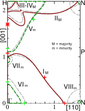
Figure 1: (color online) Left: QSGW band structure of Fe (solid lines), LSDA (grey dashed), k-point averaged QSGW (black dotted, see text), ARPES spectra Schafer05, (diamonds) and inverse photoemission spectra Himpsel91, (squares). Right: Fermi surface. Symbols denote FS crossings reported in Ref. Schafer05, . Red and green depict majority and minority $d$ character, respectively.

Fig. 1 compares the calculated QSGW band structure of Fe to peaks in ARPES spectra of Ref. Schafer05 , along with some inverse photoemission data Himpsel91 . While agreement appears to be very good, there are some discrepancies, particularly along the $\Gamma$-H line (see also Fig. 2(a)). As noted earlier, the QSGW band structure reflects the peaks of $A(\bf{k},\omega)$ with no renormalizations from the $\omega$- or $\bf{k}$- dependence of $\Sigma$.

In the FL regime, ARPES spectra $I(\bf{k},\omega)$ are generally thought to be a fairly direct measure of $A(\bf{k},\omega)$. But the two are not identical even in the FL regime, independently of the precision of the experimental setup. Assuming a one-step model pendry1976theory for the photoemission process (initial and final state coupled through Fermi’s Golden rule matzdorf1998investigation ; pendry1976theory ) $I(\bf{k},\omega)$ can be written as

$$I(\mathbf{k},\omega)\propto\int dk_{\perp}|T_{fs}|^{2}|M_{fi}(\mathbf{k}_{\bot})|^{2}A_{f}(\mathbf{k}_{\bot})A(\mathbf{k},\omega),$$ (1)

$$\hbox{where }A_{f}(\mathbf{k}_{\bot})=\frac{{\Delta k_{\bot}/2\pi}}{{(\Delta k_{\bot}/2)^{2}+(k_{\bot}-k_{\bot}^{0})^{2}}}$$

is the spectral function of the final state, broadened by scattering of the photoelectron as it approaches the surface strocov2003intrinsic . $T_{fs}$ is the final-state surface transmission amplitude and $M_{fi}$ the photoexcitation matrix element (taken to be constant and $\mathbf{k}$-independent strocov1998absolute ). Thus the final state is considered to be a damped Bloch wave, taking the form of a Lorentzian distribution centred in $k^{0}_{\perp}$ and broadened by $\Delta\mathbf{k}_{\bot}$ strocov2003intrinsic , while the initial state is an undamped Bloch function with an energy broadening $\Delta E$, obtained through the QSGW spectral function. This approximation is reasonable since in the FL regime $A(\mathbf{k},\omega)$ is sharply peaked around the QP level. $\Delta\mathbf{k}_{\bot}$ is directly related to the inverse of the electron mean free path. For photon energy in the range 100-130 eV, $\Delta\mathbf{k}_{\bot}\approx 0.2~{}$Å^-1 feibelman1974photoemission ; tanuma1994calculations .

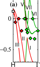
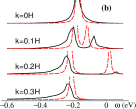
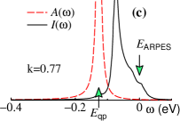
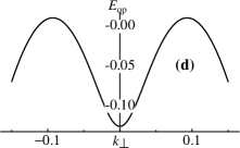
Figure 2: (a): The $\Gamma$-H line of Fig. 1 in high resolution. Labels correspond to traditional assignments of Fermi surface pockets Baraff73 ; Schafer05 . (b): Dashed line is QSGW spectral function $A(k,\omega)$ for various points on $\Gamma$-H line, with k=0 and k=1 denoting $\Gamma$ and H. Solid line is $A(\omega)$ modified according to Eq. (1). (c): the analog of ($b$) at $k{=}0.77\times$H where the II_M band crosses $E_{F}$. $E_{\rm QP}$ indicates the QSGW QP level, and $E_{\rm ARPES}$ the experimental ARPES peak at 0.77H. (d): dispersion in the QSGW II_M band on a line $\bf{k}_{\perp}$ + [0,0,0.77H] normal to the film surface.

The final-state scattering broadens $I(\omega)$; but it also can shift the peak $\bar{\omega}$ in $I(\omega)$. The most significant discrepancy between ARPES and QSGW is found in the V_m band, Fig. 2($a$) between $k{=}0$ and 0.4$\times$H. Fig. 2($b$) shows $A({\bf{k}},\omega)$ calculated by QSGW, and the corresponding $I({\bf{k}},\omega)$ calculated from Eq. (1). Estimating the peak shift change from $\delta\bar{\omega}{=}\int d\omega\,\omega I/\int d\omega I-\int d\omega\,\omega A/\int d\omega A$, we find $\delta\bar{\omega}{<}0.01$ eV at $\Gamma$, increasing to $\delta\bar{\omega}{\approx}0.06$ eV for k between 0.1H and 0.3H. $\delta\bar{\omega}$=0.06 eV tallies closely with the discrepancy between the V_m band and the measured ARPES peak for 0.1H${<}k{<}$0.3H. There is also a significant discrepancy in the II_M band near $k{=}0.77\times$H. Where it crosses $E_{F}$, the QSGW bands deviate from the ARPES peak by nearly 0.15 eV. But ARPES simulated by Eq. (1) is much closer to experiment (Fig. 2($c$)). This is understood from Fig. 2($d$), which plots the QSGW dispersion along a line $\Delta\mathbf{k}_{\perp}$ normal to the film surface, passing through [0,0,0.77H]. A measurement that includes contributions from this line biases the ARPES peak in the direction of $E_{F}$ since E_qp is minimum at ${k}_{\perp}{=}0$. Thus we attribute most of the discrepancy in the Fermi surface crossing (red star in 1($b$)) to an artifact of final-state scattering.

To better pin down the errors in QSGW, we turn to de Haas-van Alphen (dHvA) measurements. Extremal areas of the FS cross sections can be extracted to high precision from dHvA and magnetoresistance experiments. Areas normal to [110] and [111] are given in Table 1, along with areas calculated by QSGW. Fig.1 shows the QSGW Fermi surface, which closely resembles the one inferred by Lonzarich (version B) Lonzarich80 . There is some ambiguity in resolving the small VIII_m pocket at N because its tiny area is sensitive to computational details. Discrepancies in the extremal areas are not very meaningful: it is more sensible to determine the change $\Delta E_{F}$ in Fermi level needed to make the QSGW area agree with dHvA measurements. This amounts to the average error in the QSGW QP levels, assuming that the bands shift rigidly. This assumption is well verified for all pockets, except for the small VI one owing to strong electron-phonon coupling suppmat .

FS	dHvA [110]			dHvA [111]
pocket	QSGW	exptBaraff73	$\Delta E_{F}$	QSGW	exptBaraff73	$\Delta E_{F}$
I	3.355	3.3336	0.01	3.63	3.5342	0.04
II				3.694
III	0.2138	0.3190	0.05	0.1627	0.2579	0.06
IV	0.0897	0.1175	0.04	0.0846	0.1089	0.02
VI	0.3176	0.5559	-0.13	0.2799	0.4986	-0.14
VII	0.0148	0.0405	0.04
	m*/m [110]			m*/m [111]
	QSGW	LDA	exptGold71	QSGW	LDA	exptGold71
I	2.5	2.0	2.6
V				-1.7	-1.2	-1.7
VI				2.0	1.5	2.8

Table 1: de Haas-van Alphen measurements of extremal areas $A$ on the [110] and [111] Fermi surfaces, in Å^-2. $\Delta E_{F}$ is an estimate of the error in the QP level (eV), as described in the text. Bottom panel: cyclotron mass, $m^{*}/m{=}(\hbar^{2}/2{\pi}m)\,\partial{A}/\partial{E}$.

Some limited cyclotron data for effective masses are also available Gold71 , which are expected to be more reliable than ARPES data. It is seen that agreement is excellent (Table 1, bottom panel) except for the small VI pocket. We get a better comparison by accounting for the electron-phonon coupling with a simple model suppmat . From the model, $v_{F}$ is renormalized by a factor $1{+}\lambda{=}1.6$, which reasonably accounts for discrepancy between the QSGW and the cyclotron mass in pocket VI. The other pockets are much larger (Fig 1($b$)), making $v_{F}$ much larger on average, and the renormalization smaller.

Such a perfect agreement with experiments could not be possible without the accurate description of non-local components in the QSGW self-energy. To prove this statement we computed the band structure with a local potential obtained from a k-point average of the QSGW self-energy. The result is reported as a dotted black curve in Figure 1, to be compared with the pale grey lines of LSDA and the solid lines of QSGW. The k-averaged potential reproduces a band structure that is much closer to the LSDA one than to the QSGW results. This results in the overestimation of the binding energy, e.g. of most states close to Fermi (for instance at $\Gamma$), or in the range between -2 and -3 eV (see at $\Gamma$, P and H).

An additional verification that local physics is not relevant in the description of the quasiparticle structure of Fe can be found in the Supplemental Materials suppmat .

.2 Ni: an archetypical itinerant magnet

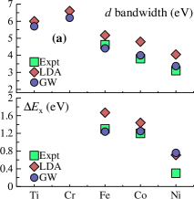
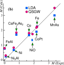
Figure 3: ($a$): $d$ bandwidth (top panel) and exchange splitting $\Delta E_{x}$ (bottom panel) in the 3$d$ elemental metals. ($b$): Magnetic moment of several compounds

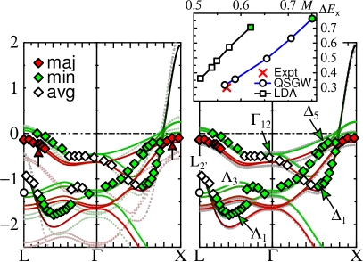
Figure 4: (color online) (left) Band structure of Ni in QSGW (solid lines) and LDA (dotted) and ARPES data HimpselNi (the circle at $-1.3$ eV was taken from Ref. Eberhardt80 ). Red arrows highlight the discrepancy in the exchange splitting $\Delta E_{x}$ at near L and X. (right) QSGW+DMFT bands with method $S$ (solid) and QSGW+$B^{\mathrm{eff}}$ (dashed). (inset) $\Delta E_{x}$ at L as a function of $M$ obtained by adding an external magnetic field to the QSGW or LSDA potential (see text).

Less detailed information is available for other elemental transition metals. We have extracted some experimental bandwidths, and also the exchange splitting $\Delta E_{x}$ in the magnetic elements. Fig. 3(a) shows that both seem to be very well described by QSGW, except that $\Delta E_{x}$ deviates strongly from experiment in Ni. QSGW significantly improves not only on the LSDA, but also on fully self-consistent GW Belashchenko06 because of loss of spectral weight in fully self-consistent $G$ that is avoided in QSGW Kotani07 .

Fig. 4($a$) compares the QSGW band structure of Ni to ARPES data HimpselNi . Agreement is excellent in the minority channel, but $\Delta E_{x}$ is uniformly too large on the symmetry lines shown. Also the band near $-1$ eV at L (consisting of $s$ character there) is traditionally assumed to be a continuation of the $d$ band denoted as white and green diamonds; but the calculations show that at it is a continuation of Ni $s$ band. The corresponding LSDA band (light dotted lines) crosses L at $E_{F}{-}0.44$ eV; also the $d$ bands are much wider.

$\Delta E_{x}$ is about twice too large in both QSGW and the LSDA, and for that reason spin wave frequencies are also too large Karlsson00a . Spin fluctuations $\left<M^{2}\right>$ are important generally in itinerant magnets but they are absent in both LSDA and QSGW. One important property they have is to reduce the average magnetic moment $\left<M\right>$ and hence to quench $\Delta E_{x}$ mazinreview ; Shimizu81 . Fig. 3($b$) shows this trend quite clearly: systems such as Fe, Co, and NiO are very well described by QSGW, but $M$ is always overestimated in itinerant magnets such as FeAl, Ni₃Al, and Fe based superconductors such as BaFe₂As₂. Ni is also itinerant to some degree (unlike Fe, its average moment probably disappears as $T{\rightarrow}T_{c}$), and its moment should be overestimated. This is found to be the case for QSGW, as Fig. 3($b$) shows.

	$M$ (Bhor)	$\Delta E_{x}$ @ L (eV)
LSDA	0.62	0.71
QSGW	0.75	0.77
QSGW+DMFT	0.51	0.30$\dagger$
QSGW+SLDMFT	0.53	0.30
QSGW+$B^{\rm eff}$	0.57	0.32
Experiment	0.57	0.31

Table 2: Magnetic moment $M$ and exchange splitting $\Delta E_{x}$ for the different levels of the theory (see text) against experiment. $\dagger$Value estimated from Maximum entropy analytic continuation.

Local spin fluctuations are well captured by localized non perturbative approaches such as DMFT. We can reasonably expect that the addition of spin-flip diagrams to QSGW would be sufficient to incorporate these effects. A $G_{0}W_{0}$+DMFT study of ferromagnetic Ni can be found in ferdiNi , but the dependency of $G_{0}W_{0}$ on the starting point, together with all the advantages mentioned at the beginning, motivated us to devise a QSGW-based approach.

Here we adopt a novel implementation merging QSGW with DMFT. We adapted Haule’s Continuous Time Quantum Monte Carlo solver with the projection and embedding schemes described in Ref. haule_prb2007 , and which are outlined in the supplemental material suppmat .

The fully consistent QSGW+DMFT calculation is composed by alternately repeated DMFT and QSGW loops. First the QSGW Green’s function is converged at fixed density, then it is projected on the Ni $d$-orbitals and finally, within the DMFT loop, the local self-energy is obtained. Updating the total density with the locally corrected Green’s function and repeating the procedure leads to complete self-consistency. This method fully takes into account the dynamics of the local spin-fluctuations included in the DMFT diagrams. Results are reported in Table 2 and they confirm that DMFT adds the correct local diagrams missing in the QSGW theory. Moreover by carefully continuing the resulting Green’s function on the real-frequency axis, we find an exchange splitting of $\sim$0.3 eV and a satellite at $\sim$5 eV suppmat .

In order to investigate the importance of the dynamics in the local spin-spin channels, we carry out a QSGW+DMFT calculation by retaining only the static limit of the DMFT loop (we call it QSGW+“SLDMFT”). Once the DMFT loop converges, we take the zero frequency limit of the magnetic part of the DMFT self-energy and add it to the spin-averaged QSGW Hamiltonian suppmat . As it is clearly shown in Table 2 and Figure 4, this static hamiltonian reproduces very accurately magnetic moment and details of the band structure. This is a strong indication that for Ni the dynamics of local spin fluctuations is not crucial. This will be the case if the quasiparticle picture is a reasonable description of Ni, even if QSGW alone does not contain enough physics to yield an optimum quasiparticle approximation.

To verify this further, we model spin fluctuations by carrying out the QSGW self-consistent cycle in the presence of a magnetic field $B^{\rm eff}$, and tuning $B^{\mathrm{eff}}$ to reduce $M$ (see inset, Figure 4) Our key finding is that when $B^{\rm eff}$ is tuned to make $M$ agree with experiment, $\Delta E_{x}$ does also, reproducing ARPES spectra to high precision in the FL regime, as clearly reported in Figure 4 and Table 2. Both the QSGW and LSDA overestimate $M$ for itinerant systems, but the latter also underestimates it in local-moment systems (Fig. 3($b$)). In the LSDA treatment of Ni, these effects cancel and render the moment fortuitously good. When spin fluctuations are folded in through $B^{\rm eff}$, the LSDA moment becomes too small. This finding must be interpreted as a sign of the superior level of internal consistency in the QSGW theory with respect to LSDA. Without such a degree of consistency spin fluctuations could not be approximated by a static field.

.3 Conclusions

We have performed detailed QSGW calculations of the electronic band structure of several 3$d$ metallic compounds to assess the reliability of this theory in the Fermi liquid regime and the importance of the non-local terms in the self-energy.

– Fe: Through de Haas-van Alphen and cyclotron measurements we established that QSGW QP levels at $E_{F}$ have an error of $\sim$ 0.05 eV, and effective masses are well described. Comparable precision is found below $E_{F}$ by comparing to ARPES data, provided final state scattering is taken into account. The QSGW $d$ bandwidth falls in close agreement with ARPES, and is approximately $0.75$ times that of the LDA (Fig. 1).

If $\Sigma$ is $k$-averaged to simulate a local self-energy, the QSGW band structure changes significantly and resembles the LDA. Thus non-locality in the self-energy is important in transition metals, and its absence explains why LDA+DMFT does not yield good agreement with ARPES  LichtensteinFe09 .

– Ni: QSGW $d$ bandwidths, the $t_{2g}{-}e_{g}$ splitting, the $s{-}d$ alignment, are all in excellent agreement with experiment, while $\langle{M}\rangle$ and $\Delta E_{x}$ are too large. However through the addition of a uniform static external field QSGW can give both in good agreement, indicating a high level of consistency in the theory, contrary to LSDA in which is not possible to have both quantities correct at the same time.

To account for spin fluctuations in an ab initio framework, we constructed a novel QSGW+DMFT implementation and we utilised it at different degrees of approximations demonstrating that in itinerant magnets as Ni (i) the dynamics of fluctuations is irrelevant (ii) their effect can be very well approximated by a static field as long as the non-local correlation part is treated accurately.

I Supplemental material

I.1 Survey on the QSGW theory

Quasiparticle self-consistency is a construction that determines the noninteracting Green’s function $G_{0}$ that is minimally distant from the true Green’s function $G$. A measure of distance, or metric is necessary; a good choice Kotani07 results in an effective static potential:

$$\bar{\Sigma}^{\rm xc}=\frac{1}{2}\sum_{ij}|\psi_{i}\rangle\left\{{{\rm Re}[\Sigma({\varepsilon_{i}})]+{\rm Re}[\Sigma({\varepsilon_{j}})]}_{ij}\right\}\langle\psi_{j}|.$$ (2)

$\Sigma_{ij}(\omega)$ is the self-energy in the basis of single-particle eigenstates $|\psi_{i}\rangle$, which becomes $iG_{0}W$ in the GW approximation. Starting from a trial $G_{0}$, e.g. the LDA, $\bar{\Sigma}^{\rm xc}$ is determined through GW, which determines a new $G_{0}$. The cycle is repeated until self-consistency.

Recently Ismail-Beigi showed that Eq. 2 also minimizes the gradient of the Klein functional, $|\delta F|^{2}$, where $F$ is evaluated in the subspace of all possible static $\bar{\Sigma}^{\rm xc}$ Ismail14 .

Another key property of Eq. 2 is that, at self-consistency, the poles of $G_{0}(\mathbf{k},\omega)$ coincide with the peaks in $G(\mathbf{k},\omega)$ . Therefore the band structure generated by $V^{\rm xc}$ coincides with the peaks of the specral function $A(\mathbf{k},\omega)$. This is significant, because it means there is no many-body “mass renormalization” of the noninteracting hamiltonian. In other words, the attribution of mass renormalization to correlation effects, a concept widely used in the literature Walter10 , is ill-defined: it depends on an arbitrary reference, e.g. the LDA. The absence of mass renormalization is a very useful property: we can directly associate QSGW energy bands $E(\bf{k})$ with peaks in the spectral function $A(\bf{k},\omega)$.

I.2 Electron-phonon renormalization of effective masses

In comparing the areas of electron pockets in the Fermi surface of Fe, we pointed out the small discrepancy between measured and simulated values. As a measure of the discrepancy we provide the rigid shift of the Fermi energy that would lead the computed area to equate the measured one (see Table II in main text). This measure is justified under the assumption that QSGW shift rigidly, which is actually not the case for pocket VI, for which the agreement is poorer.

According to a Thomas-Fermi model of screening Ashcroft76 , the elecron-phonon interaction renormalizes $v_{F}$ by a factor $1{+}\lambda$. Band VI is roughly spherical, enabling us to evaluate $\lambda$ analytically:

$$\lambda=\frac{e^{2}}{\hbar v_{F}}\left[\frac{1}{2}\ln\frac{k_{TF}^{2}}{k_{TF}^{2}+k_{F}^{2}}+\frac{k_{F}}{k_{TF}}\arctan\frac{k_{F}}{k_{TF}}\right]$$ (3)

Estimating $k_{F}{=}1.71$ Å^-1 from the Fe electron density, this leads to a renormalization factor of $1.6$.

Remembering that $v_{F}\propto 1/m*$, we can compare this factor with the ratio $m^{*}_{\rm QSGW}/m^{*}_{\rm exp}=1.4$, which is close to the estimated contribution from the electron-phonon interaction.

I.3 Computational details

I.3.1 QSGW

For the high resolution needed here, computational conditions had to be carefully controlled.

In both QSGW calculations of Fe and Ni, a $k$ mesh of 12$\times$12$\times$12 divisions was found to be sufficient for calculating $\Sigma$. The one-body part was evaluated on a 24$\times$24$\times$24 mesh.

Fe 3p and 4d states were included through local orbitals: omitting these and treating 3$p$ as core levels Kotani07 can shift QP levels by as much as 0.1 eV in the FL regime. Other parameters Kotani07 , such as broadening the pole in $G$ in constructing $\Sigma{=}iGW$, the basis of eigenfunction products, and the energy cutoff for the off-diagonal parts of $\Sigma$, were also carefully monitored. When set to tight tolerances QP levels near $E_{F}$ were stable to a resolution of 0.05 eV. QP levels are calculated including spin-orbit coupling (SOC), though it is omitted in the calculation of $\Sigma$. The effect of SOC on $\Sigma$ was found to make small changes to $\bar{\Sigma}^{\rm xc}$.

Similar parameters were used in the QSGW calculation for Ni.

I.3.2 Our QSGW+DMFT implementation

Concerning the QSGW+DMFT calculation on Ni, we projected the lattice problem on the Ni $d$ orbitals following the prescription of Haule kriproj . We compute higher level diagrams locally using the hybridization expansion version of the numerically exact continuous time QMC method werner_prl2006 ; haule_prb2007 .

In order to single out the correlated subspace, a procedure of projection/embedding which was originally introduced in kriproj in the LAPW basis of the Wien2k package, is developed in the Full-Potential Linear Muffin-Tin Orbitals (FP-LMTO) basis FPLMTO . This projector maps the full space Green’s function $G_{ij{\bf k}}$ (with band and $k$-point label $\{ij{\bf k}\}$) to the local Green’s function $G_{LL^{\prime}}^{\mathrm{loc}}$ defined only on the correlated subspace. The compact index $L\coloneqq\{\tau,R,\sigma,\ell,m\}$, collects information on the atom type $\tau$, site $R$, spin coordinate $\sigma$, and angular momentum components $\ell$ and $m$. The projection operation can be cast in the following form:

$$G_{LL^{\prime}}^{\mathrm{loc}}=\sum_{{\bf k},ij}U^{L}_{i\bf k}\,G_{ij{\bf k}}\,{U^{L^{\prime}}_{j\bf k}}^{\dagger}\quad\text{with}\quad U^{L}_{i\bf k}\propto\sum_{u}\mathcal{A}^{L}_{i\bf k}\Phi^{u}_{R\ell}\;,$$

where the coefficients $\mathcal{A}^{L}_{i\bf k}$ account for localization inside the sphere, while $\Phi^{u}_{R\ell}$ gives an estimate of correlations relative to the specific orbital component $\ell$. More specifically $\mathcal{A}^{L}_{i\bf k}$ are linear combinations of spherical harmonics $Y_{\ell m}$ and the QSGW quasiparticle eigenfunctions in the FP-LMTO basis. The terms $\Phi^{u}_{R\ell}$ are radial integral of the kind $\langle{\varphi^{u}_{R\ell}}|{\varphi_{R\ell}}\rangle$ where the index $u$ in $\varphi^{u}_{R\ell}$ indicates the possibility of selecting the radial solution $\varphi_{R\ell}$ of the Schrödinger equation inside the MTO, its energy derivative $\dot{\varphi}_{R\ell}$, and its local orbitals contributions $\varphi^{z}_{R\ell}$ Kotani07 . By means of these definitions we ensure that the localized orbitals are centred on the correlated atom corresponding to the muffin-tin site $R$.

The transformation matrices $U$ have been orthonormalised in such a way that $\sum_{i{\bf k}}{U^{L}_{i\bf k}}{U^{L^{\prime}}_{i\bf k}}^{\dagger}=\delta_{LL^{\prime}}$.

The local Green’s function is defined on a grid of Matsubara frequencies $i\omega_{n}=i\pi(2n+1)/\beta$ and it is employed to calculate the hybridization function of the system, which feeds the CTQMC impurity solver. The result of the impurity solver is the local impurity self-energy $\Sigma^{\rm loc}_{LL^{\prime}}(i\omega_{n})$ also defined on the Matsubara axis. In order to update the full Green’s function $G_{ij{\bf k}}$ with this local self-energy, so to iterate the DMFT loop to self-consistency, an embedding procedure is needed. Because of the specific properties of the transformation $U$, the embedding procedure $\Sigma^{\rm loc}_{ij{\bf k}}(i\omega_{n})=\sum_{LL^{\prime}}U^{L\dagger}_{i{\bf k}}\Sigma_{LL^{\prime}}^{\rm loc}(i\omega_{n})U^{L^{\prime}}_{j{\bf k}}$ can be operated by means of the same matrices, even though this is not a general requirement of the theory kriproj .

The charge double-counting contribution has been included by means of the standard formula

$$E_{dc}=U(n-1/2)-J(n/2-1/2)$$

where $n$ is the nominal occupancy of the $3d$ shell.

I.3.3 Analytical continuation through Maximum entropy

Figure 5: Total DOS of Fe 3$d$ states obtained from Maximum entropy method.

The output of the DMFT loop is the impurity self-energy $\Sigma^{\rm loc}_{LL^{\prime}}(i\omega)$ and the corresponding impurity Green’s function $\mathcal{G}_{LL^{\prime}}(i\omega)$. At self-consistency they correspond to the local self-energy and local Green’s function of the correlated subset ($d$-electrons of the metal in this case).

Though, since the CTQMC solver works in the Matsubara’s frequency space extrapolations to zero-energy or some kind of analytical continuation has to be employed to extract physically meaningful quantities.

We evaluated the scattering rate from the intercept at $\omega=0$ of a forth-order polynomial obtained from a fit of $\text{Im}\Sigma^{\rm loc}_{LL^{\prime}}(i\omega)$ in the vicinity of $\omega=0$. The coefficient $C_{1}$ of the linear term is then related to the quasiparticle weight $\mathcal{Z}=1/(1+C_{1})$. The intercept being $\Gamma/\mathcal{Z}$ where $\Gamma$ is the scattering rate, we have been able to evaluate $\Gamma$ between $10^{-3}$ and $10^{-4}$ for both Fe and Ni, corresponding to a coherent charge-scattering regime.

The spectral function of the correlated subset can be obtained by continuing on the real-frequency axis the quantity $A(i\omega)=-\text{Im}G_{LL^{\prime}}(i\omega)/\pi$. In order to do that, we utilised a statistical technique based on the Maximum Entropy Method gubernatis-jarrel_prb1991 . As model function we used the magnetic QSGW spectral function of the $d$ orbitals.

The resulting spectral function $A(\omega)$ contains all the effects of the dynamical local response including features beyond the quasiparticle peaks, as satellites at higher energy. This is indeed the case for Fe, reported in Figures 5.

I.3.4 Applications to Ni

In our application to Ni, the projectors used for the Ni $3d$ are constructed from 5 bands below $E_{F}$ and 3 bands above $E_{F}$, which correspond to a window of ${\sim}{\pm}10$ eV. By choosing a wide energy window, $U$ becomes nearly static Choi15 . The corresponding on-site Coulomb parameters were chosen to be $U$=10 eV and $J$=0.9 eV, as calculated by constrained RPA Choi15 . The Matsubara frequency grid is defined over 2000 points with an inverse temperature $\beta=50$ eV^-1.

In the case of Ni we applied the method at two different degrees of approximation.

Standard procedure

We first perform a full QSGW loop. Then we extract the spin-averaged Green’s function from which the local hybridization function $\Delta(i\omega_{n})$ is obtained. The DMFT solver uses $\Delta(i\omega_{n})$, $U$ and $J$ to produce the local self-energy $\Sigma^{\rm loc}_{LL^{\prime}}(i\omega_{n})$. By keeping the QSGW part of the Green’s function fixed, the calculation of the self-energy is repeated until convergence of the magnetic moment (DMFT loop). Then a new density $\rho(\mathbf{r})$ is recomputed summing over all Matsubara’s frenquencies according to

$$\rho(\mathbf{r})=\sum_{\mathbf{k},l}\left\{\frac{1}{\beta}\sum_{n=-\infty}^{+\infty}\frac{\psi^{R}_{l\mathbf{k}}(\mathbf{r},i\omega_{n})\psi^{L*}_{l\mathbf{k}}(\mathbf{r},i\omega_{n})}{i\omega_{n}+\mu-\varepsilon_{l\mathbf{k}}(i\omega_{n})}\right\}\,,$$ (4)

where $\psi^{X}_{l\mathbf{k}}(\mathbf{r},i\omega_{n})$ are the right ($X=R$) and left ($X=L$) eigenfunctions of the DMFT Hamiltonian $H_{\bf k}(i\omega_{n})$ with corresponding eigenvalues $\varepsilon_{l\mathbf{k}}(i\omega_{n})$. A new QSGW loop is then converged by keeping the density fixed, that produces a new QSGW Green’s function. The output is used to initialise a new DMFT loop and so on until QSGW self-energy and DMFT updated density are self-consistent.

The number of iterations in each DMFT loop varies between 10 and 20, and the number of random moves per iteration are roughly $10^{10}$. This method is basically the equivalent of state-of-the-art DMFT implementations in the framework of DFT+DMFT. We believe it is superior to other $G_{0}W_{0}$+DMFT implementations because of the possibility to close the full self-consistent loop and because of the higher quality of the low-level theory chosen.

QSGW+SLDMFT

From the converged DMFT self-energy, we first extrapolate the static limit of $\Sigma^{\rm loc}_{LL^{\prime}}(i\omega_{n})$, then we embed it into the lattice problem and we keep only its symmetrized real part

$$\bar{\Sigma}^{\rm loc}_{ij{\bf k}}=\text{Re}\left[\Sigma^{\rm loc}_{ij{\bf k}}(0)+\Sigma^{\rm loc}_{ji{\bf k}}(0)\right]/2.$$ (5)

This is done for the spin-up and spin-down channels separately. We finally retain only the spin-flip component $\Sigma_{2}=\bar{\Sigma}^{\rm loc}-(\bar{\Sigma}^{\rm loc}_{\uparrow}+\bar{\Sigma}^{\rm loc}_{\downarrow})/2$ and we add it to the charge component $\Sigma_{1}=(\bar{\Sigma}^{\rm xc}_{\uparrow}+\bar{\Sigma}^{\rm xc}_{\downarrow})/2$ computed at QSGW level. This procedure allowed us to prevent counting twice the magnetic contributions to the self-energy.

I.3.5 Applications to Fe

To further confirm that the local momentum is not relevant in the description of Fe, we applied the fully dynamical QSGW+DMFT approach also to Fe. The parameters $U=5$ eV and $J=0.8$ eV used are the same as inwang_natcomm2013 , where they have been derived from GW within the same projection scheme. Four valence and four conduction bands have been used to project onto the correlated system. The resulting magnetic moment $M$=2.20 Bohr, as the QSGW prediction, confirming that local corrections are absolutely negligible in Fe.

We extract the scattering rate $\Gamma$ from the intercept and the linear term of a forth-order polynomial fitting Im$\Sigma$($\omega$) in the vicinity of $\omega=0$ as explained above. We find that Fe has extremely coherent charge scattering. We also present the analytically continued ImG(i$\omega$)/$\pi$ for Fe reported in Figure 5.

References

- (1) J. Schäfer, M. Hoinkis, E. Rotenberg, P. Blaha, and R. Claessen, Phys. Rev. B 72, 155115 (2005).
- (2) J. Callaway and C. S. Wang, Phys. Rev. B16, 2095 (1977)
- (3) J. Sánchez-Barriga, et al, Phys. Rev. Lett. 103, 267203 (2009)
- (4) A. L. Walter, J. D. Riley, and O. Rader, New J. Phys. 12, 013007 (2010)
- (5) L. Hedin, J. Phys.: Condens. Matter 11, R489 (1999)
- (6) T. Kotani, M. van Schilfgaarde, and S. V. Faleev, Phys. Rev. B 76, 165106 (2007). Our code was adapted from the original ecalj code (github.com/tkotani/ecalj).
- (7) S. Ismail-Beigi, arXiv:1406.0772 (2014)
- (8) D. R. Baraff, Phys. Rev. B 8, 3439 (1973)
- (9) A. Gold, J. Low Temp. Phys. 16, 3 (1974)
- (10) A. Santoni and F. J. Himpsel, Phys. Rev. B 43, 1305 (1991)
- (11) J. Pendry, Surface Science 57, 679 (1976)
- (12) R. Matzdorf, Surface Science Reports 30, 153 (1998)
- (13) V. N. Strocov, J. Elec. Spect. and Rel. Phenomena 130, 65 (2003)
- (14) V. N. Strocov, R. Claessen, G. Nicolay, S. Hüfner, A. Kimura, A. Harasawa, S. Shin, A. Kakizaki, P. Nilsson, H. Starnberg, et al., Phys. Rev. Lett 81, 4943 (1998)
- (15) P. J. Feibelman and D. Eastman, Phys. Rev. B 10, 4932 (1974)
- (16) S. Tanuma, C. J. Powell, and D. R. Penn, Surface and Interface Analysis 21, 165 (1994)
- (17) G. G. Lonzarich, in Electrons at the Fermi surface, edited by M. Springford (Cambridge University Press, 1980)
- (18) A. V. Gold, L. Hodges, P. T. Panousis, and D. R. Stone, Int. J. Magn 2, 375 (1971)
- (19) For further details on the electron-phonon coupling model and on the QSGW+DMFT implementation and application to Fe and Ni, see Supplemental Material.
- (20) K. D. Belashchenko, V. P. Antropov, and N. E. Zein, Phys. Rev. B 73, 073105 (2006)
- (21) F. J. Himpsel, J. A. Knapp, and D. E. Eastman, Phys. Rev. B 19, 2919 (1979)
- (22) K. Karlsson and F. Aryasetiawan, Phys. Rev. B 62, 3006 (2000)
- (23) I. Mazin, D. Singh, and A. Aguyao, arXiv:cond-mat/0401563
- (24) M. Shimizu, Rep. Prog. Phys. 44, 329 (1981)
- (25) W. Eberhardt and E. W. Plummer, Phys. Rev. B 21, 3245 (1980)
- (26) S. Biermann, F. Aryasetiawan and A. Georges, Phys. Rev. Lett. 90, 086402 (2003). The main accomplishment of this work was to reproduce within GW+DMFT the satellite at -6 eV. This is also captured by LDA+DMFT LichtensteinFe09 .
- (27) K. Haule, Phys. Rev. B 75, 155113 (2007)
- (28) N. W. Ashcroft and D. Mermin, Solid State Physics (Brooks/Cole, 1976)
- (29) K. Haule, C. H. Yee, and K. Kim, Phys. Rev. B 81, 195107 (2010)
- (30) P. Werner, A. Comanac, L. de Medici, M. Troyer, and A. J. Millis, Phys. Rev. Lett. 97, 076405 (2006)
- (31) M. Methfessel, M. van Schilfgaarde and R. A. Casali, Electronic Structure and Physical Properties of Solids: The Uses of the LMTO method, Lecture Notes in Physics, vol. 535 (Springer-Verlag, Berlin, 2000)
- (32) T. Kotani, M. van Schilfgaarde, and S. Faleev, Phys. Rev. B 76, 165106 (2007)
- (33) S. Ismail-Beigi, arXiv:1406.0772 (2014)
- (34) A. L. Walter, J. D. Riley, and O. Rader, New J. Phys. 12, 013007 (2010)
- (35) N. W. Ashcroft and D. Mermin, Solid State Physics (Brooks/Cole, 1976)
- (36) J. Schäfer, M. Hoinkis, E. Rotenberg, P. Blaha, and R. Claessen, Phys. Rev. B 72, 155115 (2005).
- (37) K. Haule, C. Yee, and K. Kim, Phys. Rev. B 81, 195107 (2010)
- (38) P. Werner, A. Comanac, L. de Medici, M. Troyer, and A. J. Millis, Phys. Rev. Lett. 97, 076405 (2006)
- (39) K. Haule, Phys. Rev. B 75, 155113 (2007)
- (40) M. Methfessel, M. van Schilfgaarde and R. A. Casali, Electronic Structure and Physical Properties of Solids: The Uses of the LMTO method, Lecture Notes in Physics, vol. 535 (Springer-Verlag, Berlin, 2000)
- (41) J. E. Gubernatis, M. Jarrel, R. N. Silver and D. S. Sivia, Phys. Rev. B 44, 6011 (1991)
- (42) S. Choi, A. Kutepov, K. Haule, M. van Schilfgaarde, and G. Kotliar, arXiv:1504.07569 (2015)
- (43) Meng Wang, Chenglin Zhang, Xingye Lu, Guotai Tan, Huiqian Luo, Yu Song, Miaoyin Wang, Xiaotian Zhang, E.A. Goremychkin, T.G. Perring, T.A. Maier, Zhiping Yin, Kristjan Haule, Gabriel Kotliar, Pengcheng Dai, Nature Communications 4, 2874 (2013)