BB mode angular power spectrum of CMB from massive gravity

Abstract

The BB-mode correlation angular power spectrum of CMB is studied for primordial massive gravitational waves for several inflation models. The comparative study of the angular power spectrum with the joint BICEP2/Keck Array and Planck data suggests further constraint on the lower and upper bounds on the mass of primordial gravitons. Assuming a modified dispersion relation, the mass of primordial graviton is also calculated. The resulting constraint also agrees with other theoretical estimates.

Keywords Inflation; gravitational waves; massive gravity; cmb

1 Introduction

The force of gravity is believed to be mediated by a spin-2 particle called graviton which is commonly considered to be massless, thus travelling with the speed of light according to the theory of general relativity. However, starting with the idea of a spin-2 particle with non-zero mass, several approaches have been taken to introduce mass to graviton (Fierz and Pauli, 1939; van Dam and veltman, 1970; Zakharov, 1970; Boulware and Deser, 1972; Vainshtein, 1972; Hamed, 2004). Endowing graviton with mass leads to extra degrees of freedom which do not decouple as graviton mass approaches to zero such that the general relativistic (GR) case cannot be recovered (van Dam and veltman, 1970; Zakharov, 1970). Some of the approaches to massive gravity suffer from pathologies like the presence of ghost mode (Boulware and Deser, 1972), discontinuity when the mass approaches to zero limiting case and so on (Vainshtein, 1972), and several theories have been proposed to fix these problems and also to formulate a consistent theory of massive gravity (Hamed, 2004; Rubakov, 2004; Dubovsky, 2004; de Rham,Gabadadze and Tolley, 2011; de Rham, 2014; Hassan and Rosen, 2002). At the same time, there have been several attempts to estimate the mass of graviton from astrophysical sources as well as for primordial gravitational waves (GWs) (Goldhaber and Nieto, 1974; Talmadge, 1988; Will, 1997; Finn and Sutton, 2002; Cooray and Seto, 2004; Gershtein,Logunov and Mestvirishvili, 1997; de Rham, 2016). It is believed that if the mass of the graviton is comparable to the Hubble parameter, then the massive graviton would condensate to form effective negative pressure stress energy at cosmological distances which would provide a repulsive effect thus leading to late time cosmic acceleration, thereby suggesting that the massive gravitons could be responsible for the current accelerating phase of the universe instead of dark energy. There are also studies that propose that massive gravitons would comprise of cold dark matter as well (Dubovsky,Tinyakov and Tkachev, 2005).

In this paper, we consider the particular Lorentz-violating massive gravity theory in which the Lorentz invariance is violated through spontaneous symmetry breaking caused by the presence of background Goldstone fields which leads to the modification of the dispersion relation. The Goldstone fields are set to their vacuum values and the resulting mass parameters are fine-tuned relative to each other in such a way that the pathologies are absent, and the scalar and vector modes behave exactly like those in the general relativistic case. Hence, the modification of the gravity comes only from the tensor modes and the dispersion relation of gravitational waves acquires an effective mass and is relativistic (Rubakov, 2004; Dubovsky, 2004). According to this theory, the bound on the primordial graviton mass is obtained from the exponential decay in the Yukawa potential, putting the upper bound for the graviton mass to be $\leq 10^{-30}$ eV at the Compton wavelength of $\lambda_{g}>10^{20}$ km (Dubovsky, 2004, 2010). The lower bound for graviton mass has been proposed to be $>10^{-29}$ $cm^{-1}$ ($\equiv 1.239\times 10^{-32}$ eV) (Bessada and Miranda, 2009). The minimum for the mass of graviton in the de Sitter spacetime has also been set by the Higuchi bound as $m_{gw}^{2}\geq 2H^{2}$, where $H$ is the Hubble parameter (Fasiello and Tolley, 2012). The small mass of graviton is expected to have an effect on the temperature anisotropy and polarization spectra of the cosmic microwave background (CMB) (Dubovsky, 2010; Bessada and Miranda, 2009). The imprint of primordial gravitational waves on CMB anisotropy can be observed through the angular power spectrum of CMB in the form of B-mode polarization (Kamionkowski, Kosowsky and Stebbins, 1997; Kamionkowski and Kovetz, 2015; Baskaran, Grishchuk and Polnarev, 2006; Grishchuk, 2010). The observation of B-mode polarization on CMB can not only verify the theory of inflation itself but would also help in constraining the many inflation models (Martin, Ringeval and Vennin, 2013; Martin, 2014, 2015). The detection of B-mode polarization of CMB or the primordial GW itself would be able to provide a clear bound on the mass of primordial graviton. Hence, in this paper, we study the effect of the primordial massive GWs on the BB mode correlation angular power spectrum of CMB for various inflation models and the results are compared with the 2015 BICEP2/Keck Array and Planck collaboration data (Ade, 2015) and therefore try to obtain a constraint on the mass of primordial gravitons.

2 Massive gravitational waves

Action for massive gravity can be written in terms of the Einstein-Hilbert action and the Goldstone action as (Rubakov, 2004; Dubovsky, 2004),

$$S = S_{EH}+S_{G},$$ (1)

$$= \int d^{4}x\sqrt{-g}[-m_{pl}^{2}R+\Lambda^{4}F(Z^{ij})],$$

where $\Lambda$ characterizes the cutoff energy scale for low energy effective theory. F is a function of the Goldstone field, metric components and its derivatives. The second term in the above action leads to violation of the Lorentz symmetry. It is assumed that ordinary matter field is minimally coupled to the metric.

Action depends on the Goldstone field derivatives through the argument $Z^{ij}$ which can be obtained with the help of the following expressions,

$$Z^{ij} = X^{\gamma}W^{ij},$$

$$X = \Lambda^{-4}g^{\mu\nu}\partial_{\mu}\Phi^{0}\partial_{\nu}\Phi^{0},$$

$$W^{ij} = \Lambda^{-4}g^{\mu\nu}\partial_{\mu}\Phi^{i}\partial_{\nu}\Phi^{j}-\frac{V^{i}V^{j}}{X},$$

$$V^{i} = \Lambda^{-4}g^{\mu\nu}\partial_{\mu}\Phi^{0}\partial_{\nu}\Phi^{i},$$ (2)

where $\Phi^{0}(x)$, $\Phi^{i}(x)$, ($i=1,2,3$) are the four scalar fields and $\gamma$ is considered as a constant free parameter.

For Eq.1, the vacuum solutions corresponding to the flat Friedmann-Lemaitre-Robertson-Walker (FLRW) metric are obtained after setting the Goldstone fields to their vacuum values and can be written as

$$g_{\mu\nu} = a^{2}\eta_{\mu\nu},$$

$$\Phi^{0} = \Lambda^{2}t,$$ (3)

$$\Phi^{i} = \Lambda^{2}x^{i}.$$

where $a$ is the scale factor for the FLRW metric and $\eta_{\mu\nu}$ is the flat space metric.

The metric $g_{\mu\nu}$ with perturbations can be written as

$$g_{\mu\nu}=a^{2}\eta_{\mu\nu}+\delta g_{\mu\nu},$$ (4)

where the metric perturbations $\delta g_{\mu\nu}$ are taken after the spontaneous Lorentz symmetry breaking.

The metric perturbations can be decomposed as,

$$\delta g_{00} = 2a^{2}\varphi,$$

$$\delta g_{0i} = a^{2}(N_{i}-\partial_{i}A),$$ (5)

$$\delta g_{ij} = a^{2}[-h_{ij}-\partial_{i}Q_{j}-\partial_{j}Q_{i}+2(\psi\delta_{ij}-\partial_{i}\partial_{j}E)],$$

where $\varphi$, $\psi$, A and E are scalar fields, $N_{i}$ and $Q_{i}$ are transverse vector fields and $h_{ij}$ is the transverse-traceless tensor perturbation.

By expanding $\sqrt{-g+\delta g}$, $X(g+\delta g)$, $V^{i}(g+\delta g)$, $W^{ij}(g+\delta g)$ in Eq.2 and using Eq.1 we get the Lagrangian as

$$L_{m} = \frac{m_{pl}^{2}}{2}(m_{0}^{2}h_{00}h_{00}+2m_{1}^{2}h_{0i}h_{0i}-m_{2}^{2}h_{ij}h_{ij}$$ (6)

$$+m_{3}^{2}h_{ii}h_{jj}-2m_{4}^{2}h_{00}h_{ii}),$$

where the mass parameters are given by (Bebronne and Tinyakov, 2007),

$$m_{0}^{2} = \frac{\Lambda^{4}}{m_{pl}^{2}}[XF_{X}+2X^{2}F_{XX}],$$

$$m_{1}^{2} = \frac{2\Lambda^{4}}{m_{pl}^{2}}[-XF_{X}-WF_{W}+\frac{1}{2}XWF_{VV}],$$

$$m_{2}^{2} = \frac{2\Lambda^{4}}{m_{pl}^{2}}[WF_{W}-2W^{2}F_{WW2}],$$ (7)

$$m_{3}^{2} = \frac{\Lambda^{4}}{m_{pl}^{2}}[WF_{W}+2W^{2}F_{WW1}],$$

$$m_{4}^{2} = -\frac{\Lambda^{4}}{m_{pl}^{2}}[XF_{X}+2XWF_{XW}],$$

where

$$W = -1/3\delta_{ij}W^{ij},$$

$$\frac{\partial F}{\partial X} = F_{X},$$

$$\frac{\partial^{2}F}{\partial X^{2}} = F_{XX},$$

$$\frac{\partial F}{\partial W^{ij}} = F_{W}\delta_{ij},$$ (8)

$$\frac{\partial^{2}F}{\partial V^{i}\partial V^{j}} = F_{VV}\delta_{ij},$$

$$\frac{\partial^{2}F}{\partial W^{ij}\partial W^{kl}} = F_{WW1}\delta_{ij}\delta_{kl}+F_{WW2}(\delta_{ik}\delta_{jl}+\delta_{ij}\delta_{jk}),$$

$$\frac{\partial^{2}F}{\partial X\partial W^{ij}} = F_{XW}\delta_{ij}.$$

For the flat cosmological solutions, $X=a^{-2}\Phi^{\prime 2}$, $V^{i}=0$, $W^{ij}=-a^{-2}\delta^{ij}$. The Einstein field equations for Eq.1 with the scalar fields in the unitary gauge Eq.2 and the metric Eq.4 then reduce to the following relations,

$$\left(\frac{a^{\prime}}{a}\right)^{2} = \frac{a^{2}}{m_{pl}^{2}}[\rho_{m}+\Lambda^{4}(2XF_{X}-F)]$$ (9)

$$2\frac{a^{\prime\prime}}{a}-\left(\frac{a^{\prime}}{a}\right)^{2} = -\frac{a^{2}}{m_{pl}^{2}}[p_{m}+\Lambda^{4}(2WF_{W}+F)]$$ (10)

where $\rho_{m}$ and $p_{m}$ are the energy density and pressure respectively for ordinary matter and the equation of motion of the $\Phi^{0}$ field,

$$\partial_{0}(a^{3}F_{X}X^{1/2})=0.$$ (11)

Prime here denotes derivative with respect to conformal time $\eta$. Apart from some constraints which arise from the requirement that the model is free of ghosts and strong coupling problems, the function $F$ is quite arbitrary. Specific restrictions on the function $F$ are discussed in detail in (Dubovsky, 2004; Dubovsky,Tinyakov and Tkachev, 2005) where the existence of a wide class of functions with graviton masses are demonstrated.

The mass parameters are carefully fine tuned relative to each other. The fine tuning relations between the mass parameters characterize certain regions in the mass parameter space so that in these regions, the theory is free of pathologies, and the theory is described by a consistent low-energy effective theory with strong coupling scale $\Lambda\sim(mm_{pl})^{1/2}$ which implies a ghost-free scenario (Rubakov, 2004; Dubovsky, 2004). The mass parameter $m_{2}$ represents the mass of the graviton which arises from the modification in the tensor sector in which there are two massive spin-2 propagating degrees of freedom. The vector and scalar perturbations behave similarly as in the general relativity case.

The perturbed metric for a flat FLRW universe can be written as

$$dS^{2}=a^{2}(\eta)[-d\eta^{2}+(\delta_{ij}+h_{ij})dx^{i}dx^{j}],$$ (12)

here $\delta_{ij}$ is the flat space metric and $\eta$ is the conformal time defined by $d\eta=\frac{dt}{a}$.

The dynamical equation of motion for massive gravitational waves can be written as

$$h_{ij}^{(m)\prime\prime}(\eta)+2Hh_{ij}^{(m)\prime}(\eta)+k^{2}h_{ij}^{(m)}(\eta)+a^{2}m_{gw}^{2}h_{ij}^{(m)}(\eta)=0,$$ (13)

where $m_{gw}\equiv m_{2}$ is the mass of the graviton and $H=\frac{a^{\prime}}{a^{2}}$ is the Hubble parameter.

The massive tensor perturbation $h_{ij}^{(m)}$ can be expanded in the Fourier space as

$$h_{ij}^{(m)}(\textbf{x},\eta) = \frac{D}{(2\pi)^{\frac{3}{2}}}\int^{\infty}_{-\infty}\frac{d^{3}\textbf{k}}{\sqrt{2E_{k}}}$$

$$[h_{k}^{(m)(p)}(\eta)c_{k}^{(m)(p)}\varepsilon_{ij}^{(m)(p)}(\textbf{k})e^{i\textbf{k}.\textbf{x}}$$

$$+h_{k}^{(m)(p)\ast}(\eta)c_{k}^{(m)(p)\dagger}\varepsilon_{ij}^{(m)(p)\ast}(\textbf{k})e^{-i\textbf{k}.\textbf{x}}],$$

where $D=\sqrt{16\pi}l_{pl}$ is the normalization constant, $l_{pl}$ is the Planck length, $E_{k}$ is the energy of the mode ,$(p)$ is the polarization index and the superscript $(m)$ stands for the massive tensor perturbation.

The two polarization states $\varepsilon_{ij}^{(p)}$, $p=1,2$ are symmetric and transverse-traceless and satisfy the conditions

$\displaystyle\hskip 0.0pt{\varepsilon_{ij}^{(p)}\delta^{ij}=0,~{}~{}\varepsilon_{ij}^{(p)}k^{i}=0,}$

$\displaystyle\hskip 0.0pt{\varepsilon_{ij}^{(p)}\varepsilon^{(p^{\prime})ij}=2\delta_{pp^{\prime}},~{}~{}\varepsilon_{ij}^{(p)}(\textbf{-k})=\varepsilon_{ij}^{(p)}(\textbf{k}).}$

These polarizations are linear and are called the plus $(+)$ polarization and cross $(\times)$ polarization.

The creation and annihilation operators $c_{k}^{(p)\dagger}$ and $c_{k}^{(p)}$ satisfy the following relations

$$\left[c_{k}^{(p)},c_{k^{\prime}}^{(p^{\prime})\dagger}\right] = \delta_{pp^{\prime}}\delta^{3}(k-k^{\prime}),$$ (15)

$$\left[c_{k}^{(p)},c_{k^{\prime}}^{(p^{\prime})}\right] = \left[c_{k}^{(p)\dagger},c_{k^{\prime}}^{(p^{\prime})\dagger}\right]=0.$$ (16)

Using Eq.2 in Eq.13, we get

$$h_{k}^{(m)\prime\prime}(\eta)+2Hh_{k}^{(m)\prime}(\eta)+(k^{2}+a^{2}m_{gw}^{2})h_{k}^{(m)}(\eta)=0.$$ (17)

Hereafter we drop the polarization index $(p)$ and the index $(m)$ for notational convenience.

The mode function can be taken in the following form

$$\mu_{k}(\eta)=a(\eta)h_{k}(\eta).$$ (18)

Using Eq.18 in Eq.17 we get

$$\mu_{k}^{\prime\prime}+\left(k^{2}+a^{2}m_{gw}^{2}-\frac{a^{\prime\prime}}{a}\right)\mu_{k}=0.$$ (19)

The dispersion relation can be written as (Gumrukcuoglu, 2012)

$$\frac{k^{2}}{a^{2}}+m_{gw}^{2}=w^{2},$$ (20)

where $w$ is known as the effective frequency.

For the adiabatic vacuum, Eq.17 has the solution

$$h_{k}(\eta)\propto e^{-iwa\eta}.$$ (21)

For super horizon modes, $w^{2}\ll H^{2}$, the tensor amplitudes are frozen and the mode stays outside the horizon and its absolute value is

$$|h_{k}|=\mathcal{A}_{ex}(k),~{}~{}~{}~{}\eta<\eta_{k},$$ (22)

where $\mathcal{A}_{ex}(k)=\frac{H_{ex}}{m_{pl}k^{3/2}}$, is the amplitude of the mode at the time of its generation and $H_{ex}$ is the expansion rate at the time of horizon exit during inflation, $\eta_{k}$ is the time of horizon re-entry and $m_{pl}$ is the reduced Planck mass.

On horizon crossing, $w^{2}\simeq H^{2}$. Assuming that the horizon re-entry takes place sufficiently rapidly, i.e., $\eta\simeq\eta_{k}$, then Eq.21 can be rewritten as

$$h_{k}(\eta)=\frac{\mathcal{C}(k)}{\sqrt{w_{k}a_{k}^{3}}}e^{-iwa\eta},~{}~{}~{}~{}\eta\simeq\eta_{k},$$ (23)

where $w_{k}\equiv w(\eta_{k})=H_{k}$ indicates horizon re-entry.

On horizon re-entry, the frequency of the wave mode becomes higher than the rate of cosmic expansion, $w^{2}\gg H^{2}$, such a mode is called sub-horizon mode. Its solution is given by Eq.21:

$$h_{k}(\eta)=\frac{\mathcal{C}(k)}{\sqrt{w(\eta)a^{3}(\eta)}}e^{-iwa\eta},~{}~{}~{}~{}\eta>\eta_{k},$$ (24)

where $\mathcal{C}(k)$ is a constant of integration.

Using Eq.22, Eq.23 and Eq.24, we get

$$\frac{|h_{k}(\eta)|}{\mathcal{A}_{ex}(k)}=\sqrt{\frac{w_{k}}{w(\eta)}\frac{a_{k}^{3}}{a^{3}(\eta)}},~{}~{}~{}~{}\eta>\eta_{k}.$$ (25)

Replacing $w$ by $k/a$ and $\eta_{k}$ by $\eta_{k}^{GR}$, $GR$ indicating the massless case, we get the corresponding solution in the massless case as

$$\frac{|h_{k}^{GR}(\eta)|}{\mathcal{A}_{ex}(k)}=\frac{a_{k}^{GR}}{a(\eta)},~{}~{}~{}~{}\eta>\eta_{k}^{GR}.$$ (26)

The two-point correlation function for the massive gravitational waves can be written as

$$P(w_{0})\equiv\frac{d}{d\ln w_{0}}\langle 0|h_{ij}(\textbf{x},\eta)h^{ij}(\textbf{x},\eta)|0\rangle,$$ (27)

where

$$\langle 0|h_{ij}(\textbf{x},\eta)h^{ij}(\textbf{x},\eta)|0\rangle=\frac{D^{2}}{2\pi^{2}}\int^{\infty}_{0}k^{2}|h_{k}(\eta)|^{2}\frac{dk}{k}.$$ (28)

Therefore one gets

$$P(w_{0})=\frac{w_{0}^{2}}{w_{0}^{2}-m_{gw,0}^{2}}\frac{2k^{3}}{\pi^{2}}|h_{k}(\eta_{0})|^{2},$$ (29)

where

$$k=a_{0}\sqrt{w_{0}^{2}-m_{gw,0}^{2}},$$ (30)

$$\frac{d}{d\ln w_{0}}\left(\frac{dk}{k}\right)=\frac{w_{0}^{2}}{w_{0}^{2}-m_{gw,0}^{2}}.$$ (31)

where the subscript ’0’ represents evaluation at present time. Using Eq.25, the power spectrum for the massive gravitational waves is obtained as

$$P(w_{0}) = \frac{2k^{3}}{\pi^{2}}\mathcal{A}^{2}(k)\left(\frac{k^{\prime}a_{k}}{ka_{0}}\right)^{2}\frac{w_{k}a_{k}}{w_{0}a_{0}}$$ (32)

$$= \left(\frac{k^{\prime}a_{k}}{ka_{0}}\right)^{2}\frac{w_{k}a_{k}}{w_{0}a_{0}}P(k),$$

where $k^{\prime}=a_{0}w_{0}$ and $P(k)=\frac{2k^{3}}{\pi^{2}}\mathcal{A}^{2}(k)$ is known as the primordial power spectrum.

Using Eq.26, the power spectrum for the massless case can be written as

$$P_{GR}(w_{0})=\left(\frac{a_{k^{\prime}}^{GR}}{a_{0}}\right)^{2}P(k^{\prime}).$$ (33)

By taking the ratio of Eq.32 to Eq.33, we obtain

$$\frac{P(w_{0})}{P_{GR}(w_{0})} = \frac{P(k)}{P(k^{\prime})}\left(\frac{k^{\prime}a_{k}}{ka_{k^{\prime}}^{GR}}\right)^{2}\frac{w_{k}a_{k}}{w_{0}a_{0}}$$ (34)

$$= \frac{P(k)}{P(k^{\prime})}S^{2}(w_{0}),$$

where the enhancement factor $S(w_{0})$ can be written as

$$S(w_{0})=\frac{k^{\prime}a_{k}}{ka_{k^{\prime}}^{GR}}\sqrt{\frac{w_{k}a_{k}}{w_{0}a_{0}}}.$$ (35)

The dispersion relation at the time of horizon re-entry is

$$w_{k}\simeq m_{gw}(\eta_{k}).$$ (36)

The cosmic expansion rate is comparable to the effective mass of the gravitational waves when all modes re-enter the horizon simultaneously, then

$\displaystyle\hskip 0.0pt{H(\eta_{k})\simeq m_{gw}(\eta_{k}).}$

Therefore, we have $\eta_{k}\simeq\eta_{hc}$, $a_{k}\simeq a_{hc}$, $H_{k}\simeq H$ and $w_{hc}\simeq m_{gw}(\eta_{hc})=\frac{k_{hc}}{a_{hc}}$.

By considering the mass term which dominates the frequency modes till present time, we get

$$w_{0}\simeq m_{gw,0}=\frac{k_{0}}{a_{0}},$$

$$k^{\prime}\simeq k_{0}.$$

For long wavelength modes, the enhancement factor becomes (Gumrukcuoglu, 2012)

$$S(w_{0})\simeq\frac{a_{hc}}{a_{k_{0}}^{GR}}\sqrt{\frac{k_{hc}}{k_{0}}}\left(\frac{w_{0}^{2}}{m_{gw,0}^{2}}-1\right)^{-\frac{1}{2}}.$$ (37)

The massive short wavelength modes behave almost similar to their massless counterparts and hence, are not considered here.

3 Inflation

In the simplest inflationary scenario, the exponential expansion is driven by a canonical scalar field called the inflaton. In the slow roll scenario, the inflaton slowly rolls down its potential which is almost flat and as long as the slow-roll conditions are satisfied, inflation continues. In most models of slow-roll inflation, the inflation process ends by violation of slow-roll condition which is usually followed by decay of the inflaton and reheating. There are also several models in which the inflaton need not necessarily decay and reheating occurs via some other process.

The equation of motion for the inflaton with effective potential $V$ can be written as

$$\ddot{\phi}+3H\dot{\phi}+V^{\prime}(\phi)=0,$$ (38)

where the Hubble parameter $H$ is determined by the energy density of the scalar field,

$\displaystyle\hskip 0.0pt{\rho_{\phi}=\frac{\dot{\phi}^{2}}{2}+V,}$

so that the Friedmann equation can be written as

$$H^{2}=\frac{1}{3m^{2}_{pl}}\left(\frac{1}{2}\dot{\phi}^{2}+V(\phi)\right).$$ (39)

In the slow-roll limit, the Hubble parameter and the inflaton potential are related as

$$H^{2}\simeq\frac{V}{3m^{2}_{pl}}.$$ (40)

The slow-roll condition is characterized in terms of the slow-roll parameters defined in terms of the inflaton potential and its derivatives as follows

$$\epsilon \equiv \frac{m_{pl}^{2}}{2}\left(\frac{V^{\prime}}{V}\right)^{2},$$

$$\eta \equiv m^{2}_{pl}\left(\frac{V^{\prime\prime}}{V}\right).$$ (41)

Slow roll conditions demand that $\epsilon$, $\eta\ll 1$. As long as the slow-roll conditions are satisfied, the process of exponential expansion continues and the slow-roll approximation can be used to study the fluctuations generated during inflation. Inflation ends as soon as the slow-roll conditions are violated.

The duration of inflation is characterized by the e-folding number $N$, which can be written in terms of the potential as,

$$N\simeq\frac{1}{m_{pl}^{2}}\int_{\phi_{end}}^{\phi}\frac{V}{V^{\prime}}d\phi.$$ (42)

Throughout this paper, we use $N=60$.

There are several inflation models and most of them predict the existence of an almost scale invariant tensor perturbations or primordial gravitational waves. The tensor spectral index describes the deviation of the tensor perturbations from scale invariance and can be written in terms of the parameter $\epsilon$ as

$$n_{T}=-2\epsilon$$ (43)

The strength of the tensor fluctuations can be measured with respect to that of the scalar fluctuations and can be realized through the parameter $r$, called the tensor-to-scalar ratio as

$$r\equiv\frac{P_{T}(k)}{P_{S}(k)}\simeq 16\epsilon,$$ (44)

where $P_{T}$ and $P_{S}$ are the power spectra of the tensor and scalar perturbations respectively,

$$P_{T} = \frac{2}{3\pi^{2}m_{pl}^{4}}V,$$ (45)

$$P_{S} = \frac{1}{12\pi^{2}m_{pl}^{6}}\frac{V^{3}}{V^{\prime 2}},$$ (46)

where $V$ is evaluated at the time when the mode with the wave number $k$ crosses the horizon.

From Eq.43 and Eq.44, one can see that both $n_{T}$ and $r$ are determined by the equation of state during inflation, hence these can be very helpful in understanding the dynamics of the early universe and can also help in distinguishing the inflation models. The scalar spectral index $n_{s}$, on the other hand, must be sufficiently close to scale invariance.

3.1 Inflation models

In this work, we consider the single field slow-roll inflation models for which the corresponding tensor-to scalar ratio lies within $\mathcal{O}(10^{-3})$ and $r<0.07$ (Barenboim and Park, 2015). The scalar power spectrum for each model is taken to be $P_{S}=2.43\times 10^{-9}$.

R2 Inflation model (Starobinsky model)

This model is based on the higher order gravitational terms with the action (Asaka, 2015)

$$S=\int d^{4}x\sqrt{-g}\frac{m_{pl}^{2}}{2}\left(R+\frac{R^{2}}{6m^{2}}\right),$$ (47)

where $R$ is the Ricci scalar and $m$ is the inflaton mass.

The model can be represented in the form of Einstein gravity with a normalized inflaton field with effective potential,

$$V(\phi)=M^{4}(1-e^{-\sqrt{2/3}\phi/m_{pl}})^{2}.$$ (48)

The tensor-to-scalar ratio for this model is obtained as $r=3.25\times 10^{-3}$. The slow-roll parameters obtained for the model are

$$\epsilon = 2.03\times 10^{-4},$$

$$\eta = -1.63\times 10^{-2}.$$ (49)

The calculated tensor power spectrum with the tensor spectral index $n_{T}=-4.06\times 10^{-4}$ is $P_{T}=7.9\times 10^{-12}.$

Arctan Inflation model

This model is considered as a large field inflation where the inflaton field starts at a large value and then evolves to the minimum potential (Drees and Erfani, 2012; Drees, Erfani, 2012). The effective potential for this model is given by

$$V(\phi)=M^{4}\left[1-\arctan\left(\frac{\phi}{\mu}\right)\right],$$ (50)

where $\mu/m_{pl}=10^{-2}$ is a free parameter which characterizes the typical vacuum expectation value at which inflation takes place, $M/m_{pl}=10^{-3}$.

The tensor-to-scalar ratio for this model is found as $r=1.38\times 10^{-2}$. The calculated slow-roll parameters are,

$$\epsilon = 8.62\times 10^{-4},$$

$$\eta = 3.0\times 10^{-2}.$$ (51)

The obtained tensor power spectrum is $P_{T}=3.35\times 10^{-11}$ for which the tensor spectral index has the value $n_{T}=-1.72\times 10^{-3}$.

Higgs Inflation model

In this model, the Higgs field is considered to play the role of the inflaton. The field is considered to be non-minimally coupled to gravity(Takahasi, 2015). The effective potential for this model is

$$V(\phi)=M^{4}(1+e^{-\sqrt{2/3}\phi/m_{pl}})^{-2}.$$ (52)

The tensor-to-scalar ratio for this model is $r=2.83\times 10^{-3}$. The corresponding slow-roll parameters are,

$$\epsilon = 1.77\times 10^{-4},$$

$$\eta = -1.48\times 10^{-2}.$$ (53)

The tensor power spectrum is obtained as $P_{T}=6.87\times 10^{-12}$ with $n_{T}=-3.53\times 10^{-4}$.

Inverse Monomial Inflation model

This model is considered in the context of quintessential inflation where the inflaton need not necessarily decay and hence, may survive through the present epoch. Since the inflaton does not decay, radiation is created via gravitational particle production (Huey and Lidsey, 2001; Ratra and Peebles, 1988; Peebles and Ratra, 1988). The effective potential for this model is

$$V(\phi)=M^{4}\left(\frac{\phi}{m_{pl}}\right)^{-p},$$ (54)

where $p=3$ is a positive parameter, $M/m_{pl}=10^{-1}$.

The calculated tensor-to-scalar ratio for this model is $r=2.0\times 10^{-3}$ and the slow-roll parameters are,

$$\epsilon = 1.25\times 10^{-4},$$

$$\eta = 3.33\times 10^{-4}.$$ (55)

The tensor power spectrum is found as $P_{T}=4.86\times 10^{-12}$ with $n_{T}=-2.50\times 10^{-4}$.

Loop Inflation model

This model is studied in the context of spontaneous symmetry breaking which alters the flatness of the potential and takes the form of logarithmic function for one loop order correction (Binetruy and Dvali, 1996; Halyo, 1996; Dvali, 1996). The effective potential for this model is

$$V(\phi)=M^{4}\left[1+\alpha\ln\left(\frac{\phi}{m_{pl}}\right)\right],$$ (56)

where $\alpha=g^{2}/16\pi^{2}=0.5$ tunes the strength of radiative effects, $M=10^{16}$ GeV.

The tensor-to-scalar ratio for this model is calculated to be $r=4.34\times 10^{-2}$. The slow-roll parameters are,

$$\epsilon = 3.09\times 10^{-3},$$

$$\eta = -2.06\times 10^{-2}.$$ (57)

The tensor power spectrum is calculated to be $P_{T}=1.2\times 10^{-10}$ with the tensor spectral index $n_{T}=-6.18\times 10^{-3}$.

4 Calculations

Suppose horizon crossing occurs at time $t=t_{hc}$, then the critical momentum $k_{hc}$ when both the mass term and the momentum contribute equally to frequency is given by

$$k_{hc}=a_{hc}m_{gw}(t_{hc})=\frac{a_{hc}H_{c}}{\sqrt{2}}$$ (58)

and the scale factor at re-entry time in GR is given by

$$a_{k0}^{GR}=\frac{k_{0}}{H_{k0}^{GR}}$$ (59)

We can write Eq.37 as a function of $k$ using Eq.30 as

$$S(k)=\sqrt{2}\times 10^{-2}\left(\frac{k^{2}}{m_{gw}^{2}}\right)^{-1/2}$$ (60)

where we have assumed $H_{c}\equiv H_{k0}^{GR}$, taking the values as $k_{c}\sim 10^{-19}$ Hz and $k_{0}=2\times 10^{-18}$ Hz and dropped the subscript 0 for notational convenience.

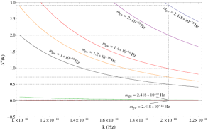
Fig. 1 : Behavior of amplification factor $S^{2}(k)$ relative to $k$ for various $m_{gw}$.

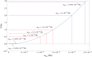
Fig. 2 : Behavior of amplification factor $S^{2}(k)$ with mass $m_{gw}$.

It can be seen from Eq.34 that $P_{T}(k)\propto S^{2}(k)$. In figures 1 and 2, we show the behavior of $S^{2}(k)$ with $k$ and mass respectively. The wave number $k$ is very small for primordial gravitational waves in the frequency range which could produce a signature on CMB with wavelength comparable to the present-day Hubble radius. As such, the evaluation is done with the wave number comparable to the same, $k\sim 2\times 10^{-18}$ Hz.

In our evaluation, we have taken $m_{gw}=2.418\times 10^{-16}~{}{\rm Hz}\equiv 10^{-30}$ eV as the upper bound for massive primordial gravitational waves and $m_{gw}=2.418\times 10^{-18}~{}{\rm Hz}\equiv 10^{-32}$ eV as the lower bound. For mass comparable to the inflationary Hubble scale ($\equiv 10^{8}$ GeV), the massive gravitons generate a blue-tilted tensor spectrum during inflation (Fujita, 2019; Wang and Xue, 2014). Also, massive spin-2 particle produces a blue tilt if $-2\epsilon+2m_{gw}^{2}/3H^{2}>0$ (Calmet, Edholm and Kuntz, 2019). Since the masses we have chosen are very small, it can be realized by straightforward calculations that for each model, we get red-tilted spectrum.

In figure 1, we show the behavior of $S^{2}(k)$ with wave number $k$ in the long wavelength regime. The vertical dashed line indicates $k=2\times 10^{-18}$ Hz. The horizontal dashed lines indicate the amplification factor for each mass at $k=2\times 10^{-18}$ Hz.

In figure 2, the blue curve represents $k=2\times 10^{-18}$ Hz. The purple lines indicate masses for which $S^{2}(k)>1$ and the red ones for $S^{2}(k)<1$. As such, masses with $S^{2}(k)>1$ will see enhancement in the spectrum while those with $S^{2}(k)<1$ will see suppression in the power level.

5 The B-mode polarization of CMB

The expression for computing the $BB$-mode correlation angular power spectrum of CMB is (Seljak and Zaldariagga, 1997; Baskaran, Grishchuk and Polnarev, 2006)

$$C_{l}^{BB} = (4\pi)^{2}\int dkk^{2}P_{T}(k)$$ (61)

$$\times\left|\int_{0}^{\eta_{0}}d\eta g(\eta)h_{k}(\eta)\Big{\{}2j^{\prime}_{l}(x)+\frac{4j_{l}(x)}{x}\Big{\}}_{x}\right|^{2}$$

where $g(\eta)=\frac{d\kappa}{d\eta}e^{-\kappa}$ is the probability distribution of the last scattering with $\kappa$ as the differential optical depth and $j_{l}(x)$ is the spherical Bessel function. The equation is evaluated at $x=k(\eta_{0}-\eta)$.

The CMB angular spectrum for the BB mode correlation with the slow-roll inflation models are obtained by using the CAMB code with $\kappa=0.08$ and $k_{0}=0.002$ Mpc^-1 as the tensor pivot scale. We generated the BB-mode $C_{l}$ data for each model using the CAMB code. Then, incorporating the massive effect, we plotted the data after adding lensing effect to the pure BB-mode. This is done so as the BKP joint data incorporates lensing effect in the errorbar.

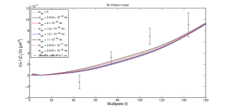
Fig. 3 : Lensed BB-mode correlation angular spectrum of CMB for the Starobinsky (R2) inflation model for various values of graviton mass with the BICEP2/Keck Array and Planck joint data.

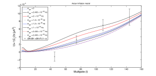
Fig. 4 : Lensed BB-mode correlation angular spectrum of CMB for the Arctan inflation model with with the recent BICEP2/Keck Array and Planck collaboration data lensing for various values of graviton mass with the BICEP2/Keck Array and Planck joint data.

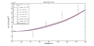
Fig. 5 : Lensed BB-mode correlation angular spectrum of CMB for the Higgs inflation model for various values of graviton mass with the BICEP2/Keck Array and Planck joint data.

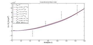
Fig. 6 : Lensed BB-mode correlation angular spectrum of CMB for the Inverse monomial inflation model for various values of graviton mass with the BICEP2/Keck Array and Planck joint data.

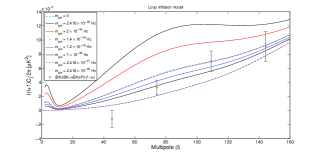
Fig. 7 : Lensed BB-mode correlation angular spectrum of CMB for the Loop inflation model for various values of graviton mass with the BICEP2/Keck Array and Planck joint data.

The obtained results are presented in figures 3, 4, 5, 6 and 7. The limit $(BK\times BK-\alpha BK\times P)/(1-\alpha)$ is taken from the BKP joint data after subtraction of dust contribution on the BICEP2/Keck Array band which is 4% times more than that in the Planck band thus giving the fiducial value $\alpha=0.04$ (Ade, 2015).

6 Conclusion and discussion

The BB mode correlation angular power spectrum of CMB for the primordial massive gravitational waves for the Starobinsky (R2), arctan, Higgs, inverse monomial and loop inflation models is studied in the context of Lorentz violating massive gravity model. Of the models studied, loop inflation model is marginally favored by constraints based on the BICEP2/Keck and Planck joint data while the rest are highly favored. The masses for which we have plotted the spectrum are those which have been previously proposed for primordial gravitational waves for consistency alongwith our own estimates where we have converted every mass unit into Hz (Dubovsky, 2004, 2010; Bessada and Miranda, 2009; Fasiello and Tolley, 2012). Note that in the figures, the enhancement around $l\sim 80$ is more model dependent rather than mass, for instance, for models with large $r$, enhancement is more. Thus, this is relative to $r$.

It is observed for each inflation model that, for gravitational waves with mass $m_{gw}\gtrsim 1.4\times 10^{-16}$ Hz, there is enhancement in the power spectrum compared to that of the massless gravitational waves case while there is decrease in the power level in the case of $m_{gw}<1.4\times 10^{-16}$ Hz. The increase/decrease in the power level of BB mode angular power spectrum of CMB for the massive gravitational waves is greater for inflation models with larger deviation ($n_{T}$) from scale invariance. The BB mode angular power spectrum of CMB for gravitational waves with mass $m_{gw}\simeq 1.4\times 10^{-16}$ Hz ($\equiv 5.79\times 10^{-31}$ eV) is found almost comparable to its massless counterpart. Hence, this is the value of the mass of primordial graviton that we have obtained.

For each slow-roll inflation model, the angular power spectrum for the gravitational waves with masses $m_{gw}=2.418\times 10^{-17}$ Hz ($\equiv 10^{-31}$ eV) and $m_{gw}=2.418\times 10^{-18}$ Hz ($\equiv 10^{-32}$ eV) are found marginally within the limit of BICEP2/Keck and Planck joint data at higher multipoles and well outside the limit at lower multipoles, which indicates that the lower limit for the graviton mass may be higher than these masses. At the same time, the upper limit for the primordial graviton mass may also be higher than $m_{gw}=10^{-30}$ eV. Hence, the results and analysis of the present study on the BB mode angular power spectrum of CMB with the BICEP2/Keck Array and Planck joint data for various inflationary models show that the mass limit for primordial graviton may be higher than the earlier proposals.

Thus, assuming a modified dispersion relation for these waves, the mass of the primordial graviton has been calculated and observed as $m_{gw}\approx 5.79\times 10^{-31}$ eV at the Compton wavelength $\lambda_{g}=2.1\times 10^{21}$ km. Our resulting estimate on the mass of the graviton is also in good agreement with other theoretical estimates (Dubovsky, 2004, 2010; Ali and Das, 2016). The present study may be repeated with other inflation models which does not seem to alter the conclusions of the present study.

Conflict of interest statement

N. Malsawmtluangi and P.K. Suresh declare that they have no conflict of interest.

Appendix A Graviton mass parameters

The quadratic Lagrangian in Eq.6 can be written in terms of the tensor, scalar and vector fields as,

$$L_{m} = m_{pl}^{2}\Big{[}-\frac{1}{4}m_{2}^{2}h_{ij}^{2}-\frac{1}{2}m_{2}^{2}(\partial_{i}Q_{j})^{2}+m_{0}^{2}\varphi^{2}+\frac{1}{2}m_{1}^{2}(\partial_{i}A)^{2}+(m_{3}^{2}-m_{2}^{2})(\partial_{i}^{2}E)^{2}$$ (A1)

$$-2(3m_{3}^{2}-m_{2}^{2})\psi\partial_{i}^{2}E+3(3m_{3}^{2}-m_{2}^{2})\psi^{2}+2m_{4}^{2}\varphi\partial_{i}^{2}E-6m_{4}^{2}\varphi\psi\Big{]}.$$

For a particular case where the equation of state parameter $w=-(3\gamma)^{-1}$ so that $\rho_{\phi}=-3\gamma p_{\phi}$, the mass parameters follow the relations,

$$m_{0}^{2} = 3\gamma\left(m_{4}^{2}-\frac{m_{1}^{2}}{2}\right),$$

$$m_{1}^{2} = 2(3\gamma-1)p_{\phi},$$ (A2)

$$m_{4}^{2} = \gamma(3m_{3}^{2}-m_{2}^{2}).$$

With the conditions $m_{0}\neq 0$ and $m_{1}\neq 0$ and $m_{4}\neq 0$, there are two scalar degrees of freedom at the linear level about the flat spacetime, one of these degrees of freedom introduces a ghost mode. Hence absence of ghost mode demands either $m_{0}=0$ or $m_{1}=0$ or both $m_{2}=m_{3}$ and $m_{4}=0$.

When $m_{0}=0$, the scalar field $\varphi$ acts as the Lagrangian multiplier which leads to the constraint,

$\displaystyle\hskip 0.0pt{2\partial_{i}\psi=m_{4}^{2}(3\psi-\partial_{i}E).}$

Thus $\psi$ remains as the only remaining dynamical scalar field and the tensor perturbation $h_{00}$ enters the action linearly. This property sufficiently ensures the ghost-free scenario.

The parameter $m_{1}$ is responsible for turning on a kinetic term for the scalar modes. When $m_{1}=0$, the scalar field $B$ acts as Lagrangian multiplier leading to the constraint for propagating modes as $\psi=0$. Applying this into the massive gravity action, it can be obtained that there are no propagating modes in the scalar sector. This property is same in the vector sector. Thus, the model is free of scalar degrees of freedom about the Minkowski at the linear level, there is no vDVZ discontinuity.

When $m_{2}=m_{3}$ and $m_{4}=0$, the field $E$ enters the action linearly leading to the corresponding field equation,

$\displaystyle\hskip 0.0pt{2\ddot{\psi}+(3m_{3}^{2}-m_{2}^{2})\psi)=0.}$

This implies the absence of high frequency propagating modes.

When the parameter $m_{2}^{2}\geq 0$, there is no rapid instabilities in the model. In the vector sector, provided $m_{2}\neq 0$, the vector field behaves in the same way as in the Einstein theory in the gauge $Q_{i}=0$; hence there are no propagating vector perturbations and gravity is not modified in this sector unless one takes into account the non-linear effects or higher derivative terms. In the scalar sector, the scalar field has massless limit which coincides with the GR expression; hence there is no vDVZ discontinuity. In the tensor sector, only the transverse-traceless perturbations $h_{ij}$ are present and their field equation is that of a massive field with the mass $m_{2}$ with helicity-2; hence there are two massive spin-2 propagating degrees of freedom. Thus, this mass parameter represents the only propagating modes under the above condition which are the tensor modes, and is called the mass of the graviton.

References

- Fierz and Pauli (1939) Fierz, M., Pauli, W, Proc. Roy. Soc. Lond. A 173 211 (1939).
- van Dam and veltman (1970) van Dam, H, Veltman, M, Nuclear Phys. B22 397 (1970).
- Zakharov (1970) Zakharov, V.I. Zh. Eksp. Teor. Fiz., Pis’ma Red Vol. 12 447 (1970).
- Boulware and Deser (1972) Boulware, D.G., Deser, S Phys. Rev. D 6 6 (1972).
- Vainshtein (1972) Vainshtein, A. I. Phys. Lett. B 22 393 (1972).
- Hamed (2004) Hamed, N. A. et.al., JHEP 0405 074 (2004).
- Rubakov (2004) Rubakov, V. arXiv:hep-th/0407104v1 (2004).
- Dubovsky (2004) Dubovsky, S. L. JHEP 0410 076 (2004).
- de Rham,Gabadadze and Tolley (2011) de Rham, C., Gabadadze, G., Tolley, A. J. Phys. Rev. Lett. 106 231101 (2011).
- de Rham (2014) de Rham, C. arXiv:1401.4173v2 [hep-th] (2014).
- Hassan and Rosen (2002) Hassan, S. F., Rosen, R. A. Phys. Rev. Lett. 108 041101 (2002).
- Goldhaber and Nieto (1974) Goldhaber, A. S., Nieto, M. M. Phys. Rev. D 9 1119 (1974).
- Talmadge (1988) Talmadge, C. et.al., Phys. Rev. Lett. 61 1159 (1988).
- Will (1997) Will, C. M. arXiv:gr-qc/9709011v1 (1997).
- Finn and Sutton (2002) Finn, L. S., Sutton, P. J. Phys. Rev. D 65 044022 (2002).
- Cooray and Seto (2004) Cooray, A., Seto, N. Phys. Rev. D 69 103502 (2004).
- Gershtein,Logunov and Mestvirishvili (1997) Gershtein, S.S., Logunov, A.A., Mestvirishvili, M. A. arXiv:hep-th/9711147v1 (1997).
- de Rham (2016) de Rham C. et.al., arXiv:1606.08462v1 [astro-ph.CO] (2016).
- Dubovsky,Tinyakov and Tkachev (2005) Dubovsky, S.L., Tinyakov P.G., Tkachev, I.I. Phys. Rev. Lett. 94 181102 (2005).
- Dubovsky (2010) Dubovsky, S. et.al, Phys. Rev. D 81 023523 (2010).
- Bessada and Miranda (2009) Bessada D., Miranda, O.D. JCAP 0908 033 (2009).
- Fasiello and Tolley (2012) Fasiello M., Tolley, A.J. JCAP 1211 035 (2012).
- Bessada and Miranda (2009) Bessada D., Miranda O.D., Class. Quant. Grav. 26 045005 (2009).
- Kamionkowski, Kosowsky and Stebbins (1997) Kamionkowski, M., Kosowsky, A., Stebbins, A. Phys. Rev. Lett. 78 2058 (1997).
- Kamionkowski and Kovetz (2015) Kamionkowski M., Kovetz E.D., arXiv:1510.06042 (2015).
- Baskaran, Grishchuk and Polnarev (2006) Baskaran, D., Grishchuk L.P., Polnarev, A.G., Phys. Rev. D 74 083008 (2006).
- Grishchuk (2010) Grishchuk, L.P. arXiv:0707.3319v4 [gr-qc] (2010).
- Martin, Ringeval and Vennin (2013) Martin, J., Ringeval C., Vennin V., arXiv:1303.3787v3 [astro-ph.CO] (2013).
- Martin (2014) Martin, J. et.al., arXiv:1312.3529v3 [astro-ph.CO] (2014).
- Martin (2015) Martin, J., arXiv:1502.05733v1 [astro-ph.CO] (2015).
- Ade (2015) Ade P.A.R. et al., Phys. Rev. Lett. 114 101301 (2015).
- Bebronne and Tinyakov (2007) Bebronne, M.V., Tinyakov, P.G., arXiv:0705.1301v2 [astro-ph] (2007).
- Gumrukcuoglu (2012) Gumrukcuoglu, A.E. et.al., Class. Quant. Grav. 29 235026 (2012).
- Barenboim and Park (2015) Barenboim, G., Park, W.I arXiV:1509.07132 [astro-ph.CO] (2015).
- Asaka (2015) Asaka, T. et.al., arXiV:1507.04344v2 [hep-th] (2015).
- Drees and Erfani (2012) Drees, M., Erfani, E. JCAP 01 035 (2012).
- Drees, Erfani (2012) Drees, M., Erfani, E. arXiv:1205.4012 [astro-ph.CO] (2012).
- Takahasi (2015) Takahasi, F. arXiv:1505.07950v1 [hep-ph] (2015).
- Huey and Lidsey (2001) Huey, G., Lidsey, J.E. Phys. Lett. B 514 217 (2001).
- Ratra and Peebles (1988) Ratra, B., Peebles, P.J.E. Phys. Rev. D 37 3406 (1988).
- Peebles and Ratra (1988) Peebles, P.J.E., . Ratra, B Astrophys. J 325 L17 (1988).
- Binetruy and Dvali (1996) Binetruy, P., Dvali, G. Phys. Lett. B 388 241 (1996).
- Halyo (1996) Halyo, E. Phys. Lett. B 387 43 (1996).
- Dvali (1996) Dvali, G. Phys. Lett. B 387 471 (1996).
- Seljak and Zaldariagga (1997) Seljak, U., Zaldariagga, M. Phys. Rev. Lett. 78 2054 (1997).
- Ali and Das (2016) Ali, A.F., Das, S. Int. J. Mod. Phys. D 25 1644001 (2016).
- Fujita (2019) Fujita, T. et. al., Phys. Lett. B 789 215 (2019).
- Wang and Xue (2014) Wang, Y., Xue, W. JCAP 10 075 (2014).
- Calmet, Edholm and Kuntz (2019) Calmet, X., Edholm, J., Kuntz, I. Eur. Phys. J. C 79 238 (2019).