Free energy of formation of clusters of sulphuric acid and water molecules determined by guided disassembly

Abstract

We evaluate the grand potential of a cluster of two molecular species, equivalent to its free energy of formation from a binary vapour phase, using a nonequilibrium molecular dynamics technique where guide particles, each tethered to a molecule by a harmonic force, move apart to disassemble a cluster into its components. The mechanical work performed in an ensemble of trajectories is analysed using the Jarzynski equality to obtain a free energy of disassembly, a contribution to the cluster grand potential. We study clusters of sulphuric acid and water at 300 K, using a classical interaction scheme, and contrast two modes of guided disassembly. In one, the cluster is broken apart through simple pulling by the guide particles, but we find the trajectories tend to be mechanically irreversible. In the second approach, the guide motion and strength of tethering are modified in a way that prises the cluster apart, a procedure that seems more reversible. We construct a surface representing the cluster grand potential, and identify a critical cluster for droplet nucleation under given vapour conditions. We compare the equilibrium populations of clusters with calculations reported by Henschel et al. [J. Phys. Chem. A 118, 2599 (2014)] based on optimised quantum chemical structures.

I Introduction

Discussions of the vapour phase often start with an ideal gas approximation, but such a viewpoint entirely ignores the existence of molecular clusters that form and dissolve as a consequence of the weak interactions that exist between the constituent particles. Were it not for these ephemeral and often disordered structures, the vapour would not easily be able to transform itself into condensed phases when prepared at lower temperatures or higher densities. The nucleation of such phases in these circumstances is determined by the kinetics of the growth and decay of molecular clusters, and considerable efforts over many years have been devoted to understanding these processes Kashchiev (2000); Ford (2004); Kalikmanov et al. (2008); Kalikmanov (2013).

Direct numerical simulation of molecular clustering in a large computational cell, necessarily with the use of empirical force fields, is increasingly being explored (e.g. Yasuoka and Matsumoto (1998); Kraska (2006); Wedekind et al. (2007); Tanaka et al. (2011); Diemand et al. (2013); Angélil et al. (2015)), though the expense is often very high and the application to complex species and realistic experimental conditions is limited. A more thermodynamic point of view is that even though nucleation is a nonequilibrium process, the population kinetics can be framed in terms of the equilibrium free energies of the molecular clusters that participate in the sequence of growth and decay events, together with timescales for collisions between clusters and monomers Ford (1997). Various modelling approaches have been used to compute cluster free energies for species present in the atmosphere, ranging from highly detailed structural studies based on quantum chemistry Kurtén and Vehkamäki (2008); Henschel et al. (2014), to semiempirical descriptions employing the continuum properties of the condensed phase Vehkamäki et al. (2002); Vehkamäki (2006); Merikanto et al. (2007). Accurate modelling of molecular clusters is a particularly difficult task, in view of their intrinsic instability and typical lack of clear structural features such as crystalline order. Small clusters can be liquid-like and descriptions made on the basis of their resemblance to solids might be questionable.

Thermodynamic techniques that make no assumption of solid-like character exist, and they have often been employed in a Monte Carlo (MC) setting Vehkamäki and Ford (2000); Merikanto et al. (2006), under constraints introduced to define an equilibrium cluster state Lee et al. (1973). Typically, MC methods involve comparisons between ensembles of similar clusters, often differing in size by one molecule, for example. A sequence of such comparisons allows us to characterise the thermodynamic properties of an arbitrary cluster, although constructing such a sequence can be laborious. Molecular dynamics approaches have also been developed Natarajan et al. (2006); Tang and Ford (2006); Julin et al. (2008) where fewer, or more natural limitations are placed upon the configurational freedom available to a cluster.

Recently, a nonequilibrium molecular dynamics (MD) method has been developed that examines the inverse of a realistic process of cluster formation in order to identify its thermodynamic stability Tang and Ford (2015). The approach employs the Jarzynski equality Jarzynski (1997), according to which the mechanical work performed on a system during a nonequilibrium process can be related to a change in equilibrium Helmholtz free energy. The method, denoted cluster disassembly, can be regarded as an MD version of thermodynamic integration Frenkel and Smit (1996) and it has some intuitively appealing features Tang and Ford (2015). External forces are used to pull a cluster apart into its constituent molecules in a controlled or guided fashion. A variation, denoted cluster mitosis, has also been developed where a cluster is separated into two subclusters, again to characterise the change in free energy associated with the process Lau et al. (2015). The methods have been successfully tested against calculations of free energies, obtained by other techniques, for model argon and water clusters.

In this paper we turn our attention to the disassembly of binary clusters. We determine what is often referred to as the free energy of cluster formation, which controls the equilibrium cluster populations in a given mixed molecular vapour. Technically, we compute the grand potential of a cluster for a given temperature and chemical potentials of the species. We study clusters of sulphuric acid and water, since this mixture has received considerable attention in connection with the formation of aerosols in the atmosphere Kuang et al. (2008); Kirkby et al. (2011); Brus et al. (2011).

In Section II we develop the theory of binary cluster disassembly and describe how the free energy change associated with such a process can be linked to equilibrium cluster populations. In Section III we discuss the MD simulations and the Jarzynski analysis that allows us to determine the free energy of disassembly. We explore two modes of disassembly processing and show that a ‘prising’ technique, where molecules are gently eased out of the cluster, has considerable advantages compared with a more straightforward separation by steady pulling that can give rise to mechanical ‘snapping’ or tearing of the cluster. In Section IV we compare our equilibrium cluster populations with calculations made by Henschel et al. Henschel et al. (2014) on the basis of minimum energy structures obtained from quantum chemistry. In Section V we give our conclusions.

II Statistical mechanics of tethered binary clusters

The external forces used in the method of cluster disassembly take the form of harmonic tethers that attach each constituent molecule of the cluster to a dedicated ‘guide’ particle, initially placed at the origin. In the molecular dynamics, the guides separate in a prescribed manner and carry their tethered molecules along with them. The mechanical work exerted by the guides on the cluster may be related to a free energy change using the Jarzynski equality. We therefore start the analysis of the disassembly by considering the free energy of a binary cluster in the presence of a weak set of harmonic tethers. We relate this to the free energy of an untethered, or free cluster, and then to the equilibrium population of the cluster in a given vapour mixture.

II.1 Free energies of free and tethered clusters

We shall represent each molecule using a single position and momentum and refer to it as a particle. The partition function of a free cluster of $N$ particles of species 1 and $M$ particles of species 2, and hence its Helmholtz free energy $F_{F}$, are given by

$$Z_{F} = \exp[-F_{F}/k_{B}T]$$ (1)

$$= \frac{1}{N!M!h^{3(N+M)}}\int\prod_{j=1}^{N}\prod_{k=1}^{M}d\boldsymbol{x}_{1j}d\boldsymbol{p}_{1j}d\boldsymbol{x}_{2k}d\boldsymbol{p}_{2k}$$

$$\times\exp[-H(\{\boldsymbol{x}_{1j},\boldsymbol{x}_{2k},\boldsymbol{p}_{1j},\boldsymbol{p}_{2k}\})/k_{B}T].$$

The dependence of the Hamiltonian $H$ on the momenta will not be noted explicitly in the following, for economy of notation. We introduce coordinates referring to the cluster centre of mass through the insertion of unity in the form of

$$1\!=\!\int\!\delta\!\left(\!\boldsymbol{x}_{c}-\frac{1}{Nm_{1}+Mm_{2}}\!\left[\sum_{j=1}^{N}m_{1}\boldsymbol{x}_{1j}+\!\sum_{k=1}^{M}m_{2}\boldsymbol{x}_{2k}\right]\right)\!d\boldsymbol{x}_{c},$$ (2)

where $m_{1}$ and $m_{2}$ are the particle masses. We hence extend the integration through the introduction of a cluster centre of mass variable $\boldsymbol{x}_{c}$, but insert a delta function constraint that categorises the molecular configurations by their centre of mass position. This is followed by a change of variables to positions of particles with respect to $\boldsymbol{x}_{c}$, namely $\boldsymbol{x}_{1j}^{\prime}=\boldsymbol{x}_{1j}-\boldsymbol{x}_{c}$ and $\boldsymbol{x}_{2k}^{\prime}=\boldsymbol{x}_{2k}-\boldsymbol{x}_{c}$. The partition function for the free cluster becomes

$$Z_{F}=\frac{1}{N!M!h^{3(N+M)}}\int\prod_{j=1}^{N}\prod_{k=1}^{M}d\boldsymbol{x}_{1j}d\boldsymbol{p}_{1j}d\boldsymbol{x}_{2k}d\boldsymbol{p}_{2k}d\boldsymbol{x}_{c}$$

$$\times\exp[-H(\{\boldsymbol{x}_{1j},\boldsymbol{x}_{2k}\})/k_{B}T]$$

$$\times\delta\!\left(\boldsymbol{x}_{c}-\frac{1}{Nm_{1}+Mm_{2}}\!\left[\sum_{j=1}^{N}m_{1}\boldsymbol{x}_{1j}+\sum_{k=1}^{M}m_{2}\boldsymbol{x}_{2k}\right]\right)$$

$$=\frac{V}{N!M!h^{3(N+M)}}\int\prod_{j=1}^{N}\prod_{k=1}^{M}d\boldsymbol{x}_{1j}^{\prime}d\boldsymbol{p}_{1j}d\boldsymbol{x}_{2k}^{\prime}d\boldsymbol{p}_{2k}$$

$$\times\exp[-H(\{\boldsymbol{x}_{1j}^{\prime},\boldsymbol{x}_{2k}^{\prime}\})/k_{B}T]$$

$$\times\delta\!\left(-\frac{1}{Nm_{1}+Mm_{2}}\!\left[\sum_{j=1}^{N}m_{1}\boldsymbol{x}_{1j}^{\prime}+\sum_{k=1}^{M}m_{2}\boldsymbol{x}_{2k}^{\prime}\right]\right),\,$$ (3)

which we can write as $Z_{F}=VZ_{F}^{c}$, where $V$ is the system volume and $Z_{F}^{c}=\exp(-F_{F}^{c}/k_{B}T)$ is the partition function for a cluster with its centre of mass fixed at the origin and $F_{F}^{c}$ is its free energy.

For a tethered cluster, the Hamiltonian will include an additional set of harmonic potentials, each designed to hold its tethered particle in oscillation at a frequency $\omega$, if isolated, irrespective of mass. We have a partition function and free energy given by

$$Z_{T} = \exp[-F_{T}/k_{B}T]$$ (4)

$$= \frac{1}{N!M!h^{3(N+M)}}\int\prod_{j=1}^{N}\prod_{k=1}^{M}d\boldsymbol{x}_{1j}d\boldsymbol{p}_{1j}d\boldsymbol{x}_{2k}d\boldsymbol{p}_{2k}$$

$$\times\exp\Biggl{[}-\Biggl{(}H(\{\boldsymbol{x}_{1j},\boldsymbol{x}_{2k}\})+\sum_{j=1}^{N}\frac{1}{2}m_{1}\omega^{2}x_{1j}^{2}$$

$$\qquad+\left.\left.\sum_{k=1}^{M}\frac{1}{2}m_{2}\omega^{2}x_{2k}^{2}\right)/k_{B}T\right],$$

and we then perform a transformation to centre of mass variables. We first write

$$\!\!\!\sum_{j=1}^{N}\frac{1}{2}m_{1}\omega^{2}x_{1j}^{2}\!+\!\sum_{k=1}^{M}\frac{1}{2}m_{2}\omega^{2}x_{2k}^{2}\!=\!\sum_{j=1}^{N}\frac{1}{2}m_{1}\omega^{2}x_{1j}^{\prime 2}\!+\!\sum_{k=1}^{M}\frac{1}{2}m_{2}\omega^{2}x_{2k}^{\prime 2}\!+\frac{1}{2}(Nm_{1}+Mm_{2})\omega^{2}x_{c}^{2}\!+\omega^{2}\!\left[\sum_{j=1}^{N}m_{1}\boldsymbol{x}_{1j}^{\prime}+\!\sum_{k=1}^{M}m_{2}\boldsymbol{x}_{2k}^{\prime}\right]\cdot\boldsymbol{x}_{c},$$ (5)

and noting that the final term can be ignored by virtue of the delta function constraint, we obtain

$$Z_{T} = \frac{1}{N!M!h^{3(N+M)}}\int\prod_{j=1}^{N}\prod_{k=1}^{M}d\boldsymbol{x}_{1j}^{\prime}d\boldsymbol{p}_{1j}d\boldsymbol{x}_{2k}^{\prime}d\boldsymbol{p}_{2k}d\boldsymbol{x}_{c}\exp\left[-\left(H\{\boldsymbol{x}_{1j}^{\prime},\boldsymbol{x}_{2k}^{\prime}\})+\Delta H\right)/k_{B}T\right]$$ (6)

$$\times\delta\left(-\frac{1}{Nm_{1}+Mm_{2}}\left(\sum_{j=1}^{N}m_{1}\boldsymbol{x}_{1j}^{\prime}+\sum_{k=1}^{M}m_{2}\boldsymbol{x}_{2k}^{\prime}\right)\right)\exp\left(-\frac{1}{2}(Nm_{1}+Mm_{2})\omega^{2}x_{c}^{2}/k_{B}T\right)$$

$$= \frac{1}{N!M!h^{3(N+M)}}\int\prod_{j=1}^{N}\prod_{k=1}^{M}d\boldsymbol{x}_{1j}^{\prime}d\boldsymbol{p}_{1j}d\boldsymbol{x}_{2k}^{\prime}d\boldsymbol{p}_{2k}\exp\left[-H(\{\boldsymbol{x}_{1j}^{\prime},\boldsymbol{x}_{2k}^{\prime}\})/k_{B}T\right]$$

$$\times\left[\frac{2\pi k_{B}T}{(Nm_{1}+Mm_{2})\omega^{2}}\right]^{3/2}\exp(-\Delta H/k_{B}T)\,\delta\left(-\frac{1}{Nm_{1}+Mm_{2}}\left(\sum_{j=1}^{N}m_{1}\boldsymbol{x}_{1j}^{\prime}+\sum_{k=1}^{M}m_{2}\boldsymbol{x}_{2k}^{\prime}\right)\right)$$

$$= \left[\frac{2\pi k_{B}T}{(Nm_{1}+Mm_{2})\omega^{2}}\right]^{3/2}Z_{T}^{c},$$

where $\Delta H=\sum_{j=1}^{N}\frac{1}{2}m_{1}\omega^{2}x_{1j}^{\prime 2}+\sum_{k=1}^{M}\frac{1}{2}m_{2}\omega^{2}x_{2k}^{\prime 2}$ and $Z_{T}^{c}=\exp(-F_{T}^{c}/k_{B}T)$ is the partition function of a cluster in the presence of tethering potentials and with its centre of mass constrained to lie at the origin.

We shall treat the tethering terms in Eq. (6) as a perturbation. We write $F_{T}^{c}\approx F_{F}^{c}+\langle\Delta H\rangle_{0}$ where $F_{F}^{c}$ is the free energy of the free cluster with its centre of mass constrained to lie at the origin, and the suffix 0 indicates that the expectation value is to be taken in an ensemble of such clusters. We introduce single particle radial density profiles $\rho_{NM}^{1}(x_{1}^{\prime})$ and $\rho_{NM}^{2}(x_{2}^{\prime})$ for each species in an $(N,M)$ cluster according to such an ensemble and write

$$\langle\Delta H\rangle_{0} = \frac{N}{2}\int\rho_{NM}^{1}(x_{1}^{\prime})m_{1}\omega^{2}x_{1}^{\prime 2}d\boldsymbol{x}_{1}^{\prime}$$ (7)

$$+\frac{M}{2}\int\rho_{NM}^{2}(x_{2}^{\prime})m_{2}\omega^{2}x_{2}^{\prime 2}d\boldsymbol{x}_{2}^{\prime},$$

so that the difference in free energy between the free and tethered cluster is:

$$F_{F}-F_{T}=\Delta F_{T}=-k_{B}T\ln[\rho_{c}^{NM}(0)V]$$ (8)

$$\!\!-\frac{N}{2}\!\int\!\rho_{NM}^{1}(x_{1}^{\prime})m_{1}\omega^{2}x_{1}^{\prime 2}d\boldsymbol{x}_{1}^{\prime}\!-\frac{M}{2}\!\int\!\rho_{NM}^{2}(x_{2}^{\prime})m_{2}\omega^{2}x_{2}^{\prime 2}d\boldsymbol{x}_{2}^{\prime},$$

where we have introduced $\rho_{c}^{NM}(0)=[(Nm_{1}+Mm_{2})\omega^{2}/(2\pi k_{B}T)]^{3/2}$, which can be regarded as an inverse volume associated with the motion of the centre of mass of the tethered cluster about the origin. The first term on the right hand side of Eq. (8) is a correction to the entropy of the cluster brought about by the tethering, while the remaining terms are corrections to the energy.

II.2 Grand potential and equilibrium cluster densities

We now introduce the grand potential of a free $(N,M)$ cluster, defined by

$$\Omega_{NM}(T,\mu_{1},\mu_{2})=F_{F}(N,M)-N\mu_{1}-M\mu_{2},$$ (9)

where $\mu_{1}$ and $\mu_{2}$ are the chemical potentials of the particle bath for the two species. The equilibrium densities of clusters in a binary vapour phase can be shown Ford (1997) to be given by $n_{NM}=V^{-1}\exp(-\Omega_{NM}/k_{B}T)$. We could express $n_{NM}$ in terms of the density of a monomer of either species 1 or 2, so that, for example, $n_{NM}=n_{10}\exp(-(\Omega_{NM}-\Omega_{10})/k_{B}T)$ in terms of the grand potential difference $\Omega_{NM}-\Omega_{10}=F_{F}(N,M)-F_{F}(1,0)-(N-1)\mu_{1}-M\mu_{2}$, but it is more straightforward to proceed without introducing the grand potential of a monomer.

Representing the particle bath as a mixture of ideal gases with readily calculable chemical potentials, the cluster grand potential is

$$\Omega_{NM}=F_{F}(N,M)-Nk_{B}T\ln(\Lambda_{1}n_{1})-Mk_{B}T\ln(\Lambda_{2}n_{2}),$$ (10)

where we introduce bath monomer densities $n_{1}=n_{10}$ and $n_{2}=n_{01}$, and where $\Lambda_{s}=[h^{2}/(2\pi m_{s}k_{B}T)]^{3/2}$ for $s=1,2$. Next, we consider the free energy difference $\Delta F_{D}=F_{f}-F_{T}$ between the disassembled, but still tethered, constituent particles and the tethered cluster. $F_{f}$ is the combined free energy of $N$ harmonic oscillators of species 1 and $M$ harmonic oscillators of species 2, which can be written as:

$$F_{f}=-3k_{B}T\left[N\ln\left(\frac{k_{B}T}{\hbar\omega_{f1}}\right)+M\ln\left(\frac{k_{B}T}{\hbar\omega_{f2}}\right)\right],$$ (11)

where $\omega_{fs}=(\kappa_{f}/m_{s})^{1/2}$ is the oscillator frequency of species $s$, written in terms of a final value of the tethering strength $\kappa_{f}$ and the particle mass. In the MD procedure, the free energy of disassembly that we extract is actually $\Delta F_{{\rm MD}}=F_{f}-F_{T}^{{\rm dist}}$ since particles are distinguishable in MD. The partition functions for distinguishable and indistinguishable particles are related through $Z_{T}^{{\rm dist}}=N!M!Z_{T}$ and thus

$$\Delta F_{{\rm MD}}=\Delta F_{D}+k_{B}T\ln N!+k_{B}T\ln M!,$$ (12)

so we can write the dimensionless grand potential of a free $(N,M)$ cluster as

$$\Omega_{NM}/k_{B}T = -3\left[N\ln\left(\frac{k_{B}T}{\hbar\omega_{f1}}\right)+M\ln\left(\frac{k_{B}T}{\hbar\omega_{f2}}\right)\right]$$ (13)

$$-\Delta F_{{\rm MD}}/k_{B}T+\ln(N!M!)+\Delta F_{T}/k_{B}T$$

$$-N\ln(\Lambda_{1}n_{1})-M\ln(\Lambda_{2}n_{2}).$$

This gives

$$\frac{\Omega_{NM}}{k_{B}T} = -N\ln(n_{1}v_{{\rm HO}})-M\ln(n_{2}v_{{\rm HO}})$$ (14)

$$-\Delta F_{{\rm MD}}/k_{B}T+\ln(N!M!)-\ln\left[\rho_{c}^{NM}(0)V\right]$$

$$-\frac{N}{2k_{B}T}\int\rho_{NM}^{1}(x_{1}^{\prime})\kappa_{i1}x_{1}^{\prime 2}d\boldsymbol{x}_{1}^{\prime}$$

$$-\frac{M}{2k_{B}T}\int\rho_{NM}^{2}(x_{2}^{\prime})\kappa_{i2}x_{2}^{\prime 2}d\boldsymbol{x}_{2}^{\prime},$$

where $v_{{\rm HO}}=(2\pi k_{B}T/\kappa_{f})^{3/2}$ with $\kappa_{f}=m_{1}\omega_{f1}^{2}=m_{2}\omega_{f2}^{2}$ is a volume representing the freedom of motion of each particle about its guide after disassembly. The final tether strengths are taken to be the same for both species, and the mass dependent initial tether strengths $\kappa_{i1}$ and $\kappa_{i2}$ have been inserted into the last two terms.

When $M=0$, the expressions reduce to those previously derived for the single species case Tang and Ford (2015). We find that the grand potential, correctly, has no dependence on $\hbar$ and the equilibrium cluster density $n_{NM}=\exp(-(\Omega_{NM}+k_{B}T\ln V)/k_{B}T)$ does not depend on the system volume $V$. Note that the equilibrium cluster densities can be expressed in terms of the chemical potential of a saturated vapour mixture if so desired, which is the traditional way to proceed in nucleation theory, but here we avoid such a representation and consider their dependence on the monomer densities $n_{1}$ and $n_{2}$ rather than the saturated densities.

The analysis of binary clusters could easily be extended to clusters of an arbitrary number of species, if such systems are of interest. In the next section we turn our attention to determining the free energy of disassembly $\Delta F_{{\rm MD}}$ using MD simulation and the Jarzynski equality.

III Determining the free energy of disassembly of binary clusters

III.1 Simulation details and data analysis using the Jarzynski equality

We employ a method for cluster disassembly based upon that developed in earlier work Tang and Ford (2015). We study clusters of sulphuric acid and water, ranging in size from dimers up to a cluster of twelve molecules. Each molecule is harmonically tethered, initially weakly, to one of a set of guide particles located at the origin. The tethering force is applied to the heaviest atom in each molecule, namely the sulphur in sulphuric acid and the oxygen in water. A preparatory MD run of 10.5 ns duration is carried out under $NVT$ conditions in which the system is allowed to equilibrate at 300 K in the presence of tethering and intermolecular interactions. For the sulphuric acid we used a set of classical interaction potentials developed by Loukonen et al. Loukonen et al. (2010) based on a series of quantum chemistry calculations, and the water was described by the SPC/E-F extended simple point charge model Yuet and Blankschtein (2010).

An ensemble of 1000 equilibrium configurations was selected at intervals of 0.01 ns from the equilibrated trajectory, rejecting a very few where a water molecule had temporarily become detached from the cluster. A further set of simulations was then carried out, in which the equilibrated clusters were disassembled through programmed motion of the guide particles along with variation in the strength of the harmonic tethers. Such a trajectory over a time interval $\tau$ provides a work of disassembly given by

$$W = \frac{1}{2}\int\limits_{0}^{\tau}\frac{d\kappa_{1}(t)}{dt}\sum_{j=1}^{N}\left[\hat{\boldsymbol{x}}_{1j}(t)-\mathbf{X}_{1j}(t)\right]^{2}dt$$ (15)

$$-\int\limits_{0}^{\tau}\kappa_{1}(t)\sum_{j=1}^{N}\left[\hat{\boldsymbol{x}}_{1j}(t)-\mathbf{X}_{1j}(t)\right]\cdot\mathbf{V}_{1j}(t)\,dt$$

$$+\frac{1}{2}\int\limits_{0}^{\tau}\frac{d\kappa_{2}(t)}{dt}\sum_{k=1}^{M}\left[\hat{\boldsymbol{x}}_{2k}(t)-\mathbf{X}_{2k}(t)\right]^{2}dt$$

$$-\int\limits_{0}^{\tau}\kappa_{2}(t)\sum_{k=1}^{M}\left[\hat{\boldsymbol{x}}_{2k}(t)-\mathbf{X}_{2k}(t)\right]\cdot\mathbf{V}_{2k}(t)\,dt,\quad$$

where $\kappa_{s}(t)$ is the time dependent strength of the tether attached to species $s$, $\hat{\boldsymbol{x}}_{sm}$ is the position of the heavy atom in the $m$th molecule of species $s$, and $\mathbf{X}_{sm}$ and $\mathbf{V}_{sm}$ are the position and velocity of the associated guide particle.

We employ the Jarzynski equality to relate the work to the shift in free energy brought about by the change in Hamiltonian associated with evolution from the initial to the final state of the system. This relationship is $\Delta F_{{\rm MD}}=-k_{B}T\ln\langle\exp(-W/k_{B}T)\rangle$ where the angled brackets represent an average over the ensemble of disassembly trajectories Jarzynski (1997). In principle, the free energy change extracted in this way should not depend on the protocol of disassembly, but in practice there can be a remnant dependence arising from limited statistical coverage of the range of trajectories, and we shall consider examples of such dependence in Section III.2.

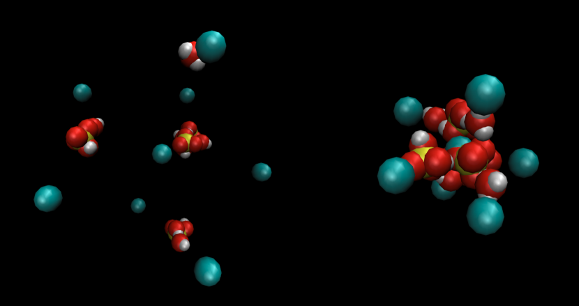
Figure 1: Illustrations of intermediate stages in the disassembly of an $N_{W}=4$, $N_{A}=4$ cluster of sulphuric acid and water. In the image on the left, representing the simple pulling scheme, the tethers between the guide particles (large spheres) and the molecules are significantly stretched, while on the right, taken from a prising simulation, molecules are eased out of the cluster by guides situated at close range with increasing tether strength. Movies of these disassembly trajectories are provided in the supplemental material.

Simulations were performed using a version of the DL_POLY molecular dynamics package Todorov et al. (2006), modified to implement the time dependent harmonic tethering potentials. The molecules, but not the guides, were coupled to a Langevin thermostat with a friction coefficient of 0.1 ps^-1. We carried out the disassembly procedure on a set of 46 clusters at 300 K, with the number of water molecules, $N_{W}$, and the number of sulphuric acid molecules, $N_{A},$ ranging from 0 to 6, excluding the cases of a monomer of either species (these labels correspond to $N$ and $M$, respectively, in the previous expressions). During the simulation, one of the guide particles remains at the origin, while all others are distributed uniformly on a sphere Sloane et al. (2000) of time dependent radius appropriate to the disassembly protocol. The timestep employed in all cases was 1 fs.

The initial oscillator frequencies for each species are required to be the same, implying mass dependent initial tether strengths satisfying $\kappa_{iW}/\kappa_{iA}=m_{W}/m_{A}$. We employ a reference initial tether strength $\bar{\kappa}_{i}$ of 0.09 kJ mol^-1Å^-2. This is small enough that the elevation in energy for a molecule at the edge of the cluster is less than $k_{B}T$ Tang and Ford (2015), and slight variations have been shown elsewhere Lau et al. (2015) to have little effect on the extracted cluster free energy. We define $\kappa_{iW}=2\bar{\kappa}_{i}m_{W}/M_{WA}$ and $\kappa_{iA}=2\bar{\kappa}_{i}m_{A}/M_{WA}$, where $M_{WA}=m_{W}+m_{A}$. Examples of cluster configurations during disassembly, together with their guide particles, are shown in Figure 1.

III.2 Optimising the disassembly protocol

We considered two modes of cluster disassembly, and implemented each for a range of separation times to examine the convergence of the free energy of disassembly. We first carried out a simple pulling protocol in which the guide particles separate at a constant speed for the duration of the simulation. The tethers start to tighten after 20% of the total separation time and reach their maximum strength at 80%, in a fashion that was successfully employed in the disassembly of argon clusters Tang and Ford (2015). The radius of the sphere on which all but one of the guide particles are finally distributed is 25 Å, and the ultimate value of the tether strength is 0.60 kJ mol^-1Å^-2. The final guide particle separation was such that the tethered molecules did not interact significantly with one another and the mean work performed during the separation had saturated.

However it became apparent that simple pulling typically disassembled a cluster through a sequence of abrupt ‘snapping’ events. Molecules showed a reluctance to separate from the cluster, indicated by an increase in the tether length as its guide particle moved away. This is illustrated in the left hand image in Figure 1. When the force on the molecule was strong enough to remove it from the cluster, the guide particle had moved so far away that the extracted molecule, after a short relaxation period characteristic of the thermostat, had little further interaction with the cluster. Mechanically, these extractions were typically irreversible, which also implied a thermodynamic irreversibility, in the sense that a significant fraction of the exerted work was converted into heat and passed to the heat bath. The contrast with argon cluster separation in earlier work Tang and Ford (2015) was brought about by the stronger intermolecular interactions in the present system.

Consequently, a second protocol that we call ‘prising’ was developed to overcome these problems. It consists of the following stages, where $\tau$ is the separation time:

• $t\leq 0.1\,\tau$: Motion of the guide particles to a distance of 7.5 Å from the origin, at constant initial tether strength.

• $0.1\,\tau<t\leq 0.6\,\tau$: Guide particles are held stationary, while tethers tighten to $\kappa_{f}$ = 3.80 kJ mol^-1Å^-2.

• $0.6\,\tau<t$: Separation of the guide particles to final positions on a sphere of radius 10.5 Å, at constant tether strength.

The motivation for this procedure is that if the guide remains in position as the tethers tighten, a molecule can be separated from the cluster but remains close enough to allow interaction and also re-attachment. The image on the right hand side of Figure 1 illustrates a typical configuration from the middle stage in the prising sequence. Once the tethers are fully tightened and the molecules prised or eased out of the cluster, having explored a variety of ways of doing so, the guides resume their outward motion, although we found that little further work was performed, on average, in the third stage: the molecules had by then been sufficiently separated (in contrast to the 25 Å employed in the simple separation scheme with much weaker tethering). The firm but more reversible removal of the molecules from the cluster would be expected to lead to lower variance in the work of disassembly.

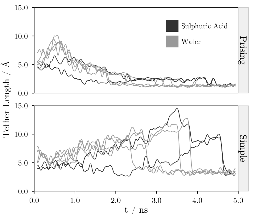
Figure 2: The evolution of tether lengths, defined as the distance between the tethered atom and its associated guide, for the two disassembly schemes. The cluster consists of $N_{W}=4$, $N_{A}=2$ molecules and is separated over a time of 5 ns. Note the sharp and irreversible ‘snapping’ of particles out of the cluster towards their guides in the simple pulling scheme, for example at $t\approx 3.6$ ns. The data have been smoothed using a Gaussian filter of width 0.15 ns.

The difference between the simple pulling and the prising protocols is illustrated in Figure 2 for the disassembly of a cluster of four waters and two sulphuric acid molecules over a period of 5 ns. The lengths of a set of tethers, defined as the distance between the guide and the atom to which it is attached, smoothed using a Gaussian filter of width 0.15 ns to remove some of the noise, are shown evolving in time for both protocols. The snapping behaviour in the simple pulling protocol is evident in the form of an increasing extension of the tethers followed by a rapid decrease. For the prising case, the there is more hopping of molecules between the guide and the cluster, and the general shortening of the tether length with time is a consequence of the progressive tether tightening. A movie that shows the irreversible snapping of a $N_{W}=4$, $N_{A}=4$ cluster during the simple pulling mode of disassembly is available in the supplemental material, together with a movie of the prising scheme.

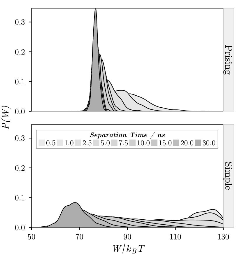
Figure 3: Kernel density estimates Scott (1992) for the distribution of work $W$ (approximate probability density functions and hence denoted $P(W)$) for the disassembly of a $N_{W}=4$, $N_{A}=2$ cluster, for a range of separation times and for both disassembly schemes. Note the faster convergence and the lower variance for the prising disassembly protocol.

Work distributions and the extracted free energies of disassembly are shown in Figures 3 and 4, respectively, for the $N_{W}=4$, $N_{A}=2$ cluster and covering a range of separation times for both disassembly protocols. There is a clear reduction of the variance in work and of the simulation time required for convergence of the free energy of disassembly $\Delta F_{{\rm MD}}$ when using the prising protocol. Note that the final tether strength in the prising protocol is higher than for simple pulling, so the converged free energy changes are not expected to be the same for the two approaches. The most important feature of Figure 4 is that converged values of $\Delta F_{{\rm MD}}$ are obtained for shorter simulations using the prising technique. We present grand potentials of cluster formation in the next section based on a prising separation time of 15 ns, although shorter times could be used without significant loss of accuracy.

Figure 4: Estimates of the free energy of disassembly $\Delta F_{{\rm MD}}$ for a $N_{W}=4$, $N_{A}=2$ cluster, for the two disassembly schemes and for a range of separation times. Error bars are the standard error in the mean based on 1000 independent trajectories. The prising scheme offers better convergence and reduced errors. Note that we should not expect the values of $\Delta F_{{\rm MD}}$ to be the same for each protocol, due to the difference in final tether strength.

IV Comparison with harmonic quantum chemical approach

We now combine the theoretical development given in Section II (specifically Eq. (14)) with the numerical evaluations of the free energy of disassembly discussed in Section III. We also require single particle radial density profiles $\rho_{NM}^{s}$ of a free cluster about its centre of mass, in order to evaluate the integrals $\int\rho_{NM}^{s}(x_{s}^{\prime})x_{s}^{\prime 2}d\boldsymbol{x}_{s}^{\prime}$ in Eq. (14). As an approximation, we computed these numerically using the initial configurations of clusters in the presence of weak tethers prior to disassembly. In Figure 5 we present the grand potential of clusters containing up to six molecules of each species. We employ sulphuric acid and water monomer densities of $2.804\times 10^{-9}$ and $8.531\times 10^{-8}$ Å^-3 respectively, ($2.804\times 10^{15}$ and $8.531\times 10^{16}$ cm^-3 in more commonly used units) which were chosen to make the deviations of the surface from planarity most apparent. The surface has a saddle point and hence a critical cluster at $N_{A}\approx 4$ and $N_{W}\approx 3$ for this case.

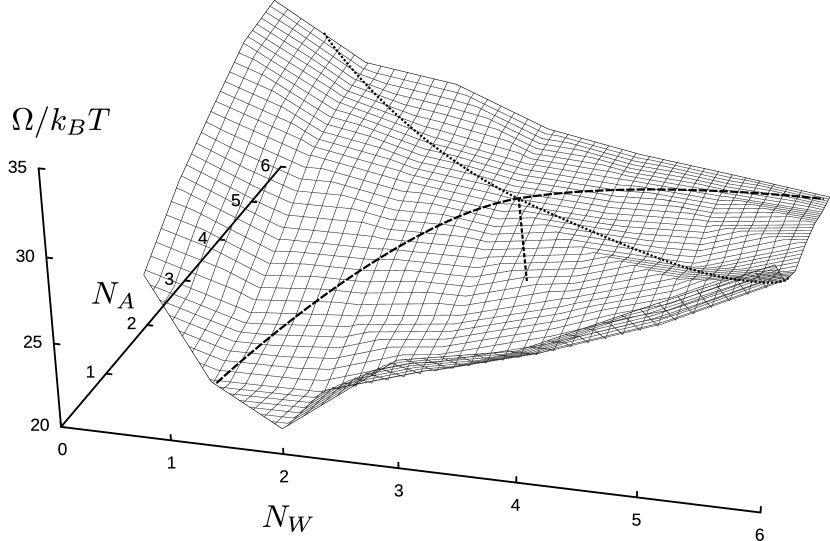
Figure 5: A surface representing the grand potential for all clusters considered, based on sulphuric acid and water monomer densities of $2.80\times 10^{-9}$ and $8.53\times 10^{-8}$ Å^-3, respectively, and with $T=300$ K. The constrained equilibrium density of ($N_{W},N_{A}$) clusters is given by $\exp(-\Omega/k_{B}T)$ in units of Å^-3. The mesh is interpolated between integer values of molecular numbers using a 3rd-order spline interpolation. Approximate lines of steepest descent and ascent are overlaid and the critical cluster lies at the saddle point where they cross. An interactive version of this plot is available as a CDF file in the supplemental material.

It should be emphasised that these monomer densities do not correspond to conditions for observed particle nucleation Kirkby et al. (2011); Almeida J, Schobesberger S, Kürten A, et al. (2013). The acid monomer density is several orders of magnitude higher than the typical range of $10^{6}-10^{8}$ cm^-3 for sulphuric acid in the atmosphere at 300 K Almeida J, Schobesberger S, Kürten A, et al. (2013). It is likely that atmospheric particle nucleation proceeds with the participation of additional molecular species, so we do not expect to find that our model reproduces such events. Furthermore, it is quite possible that the microscopic interactions used in this study are in need of improvement: an extended model that permits proton transfer has recently been developed and could be used to rectify some of its deficiencies Stinson et al. (2016). A similar situation was encountered in the earlier demonstration of the cluster disassembly procedure for a single species, argon Tang and Ford (2015). The extracted cluster thermodynamic properties were consistent with other studies that used the same Lennard-Jones interactions, but the implied correspondence with experimental nucleation rates for that substance was known to be poor Iland et al. (2007); Kalikmanov et al. (2008). Similarly, we place emphasis here on the successful implementation of the disassembly procedure and the determination of cluster thermodynamic properties starting from a molecular interaction scheme rather than a presentation of realistic correlation with data. Indeed, such is the sensitivity of cluster populations to details of the interactions, we tend to regard a comparison with data to be informative of the molecular interactions rather than predictive of the experimental outcomes.

The extracted thermodynamic information can be used as the basis of a kinetic theory of binary nucleation Reiss (1950); Wilemski and Wyslouzil (1995); Vehkamäki (2006) but our main objective is to compare the results with a recent thermodynamic analysis based on optimised cluster configurations and harmonic thermal fluctuations obtained from quantum chemistry Henschel et al. (2014). We expect differences in outcomes since the force field we use is a classical representation of quantum mechanical interactions and might lack detail such as a description of molecular dissociation (though this can be remedied Stinson et al. (2016)), but equally, the harmonic approach might not capture the correct entropic contributions to the cluster free energy since it is fundamentally based on a solid-like conception of each structure. We compare the approaches by computing the equilibrium populations of clusters. Technically, these would be clusters in a constrained equilibrium where detailed balance is artificially maintained between the growth and decay of clusters of all sizes and compositions. Under the correct kinetics, cluster populations in a stationary state of steady nucleation may be related to these equilibrium populations.

We evaluate populations normalised by the populations of clusters with the same number of acid molecules but no waters, namely $n_{NM}/n_{0M}$, in order to make a direct comparison with numerical data presented by Henschel et al. Henschel et al. (2014). Since $n_{NM}=V^{-1}\exp(-\Omega_{NM}/k_{B}T)$ we have $n_{NM}/n_{0M}=\exp[-(\Omega_{NM}-\Omega_{0M})/k_{B}T]$, which for $M\neq 1$ involves

$$\frac{\Omega_{NM}-\Omega_{0M}}{k_{B}T}=-N\ln(n_{1}v_{{\rm HO}})-\frac{\Delta F_{{\rm MD}}(N,M)}{k_{B}T}+\ln N!$$

$$-\ln\left[\frac{\rho_{c}^{NM}(0)}{\rho_{c}^{0M}(0)}\right]-\frac{N}{2k_{B}T}\int\rho_{NM}^{1}(x_{1}^{\prime})\kappa_{i1}x_{1}^{\prime 2}d\boldsymbol{x}_{1}^{\prime}$$

$$-\frac{M}{2k_{B}T}\int\rho_{NM}^{2}(x_{2}^{\prime})\kappa_{i2}x_{2}^{\prime 2}d\boldsymbol{x}_{2}^{\prime}+\frac{\Delta F_{{\rm MD}}(0,M)}{k_{B}T}$$

$$+\frac{M}{2k_{B}T}\int\rho_{0M}^{2}(x_{2}^{\prime})\kappa_{i2}x_{2}^{\prime 2}d\boldsymbol{x}_{2}^{\prime},$$ (16)

while for $M=1$ we can write $n_{N1}/n_{01}=\exp[-\Omega_{N1}/k_{B}T-\ln(n_{01}V)]$ and use

$$\frac{\Omega_{N1}}{k_{B}T}+\ln(n_{01}V)=-N\ln(n_{01}v_{{\rm HO}})-\ln(\rho_{c}^{N1}(0)v_{{\rm HO}})$$

$$-\frac{\Delta F_{{\rm MD}}(N,1)}{k_{B}T}+\ln N!-\frac{N}{2k_{B}T}\int\rho_{N1}^{1}(x_{1}^{\prime})\kappa_{i1}x_{1}^{\prime 2}d\boldsymbol{x}_{1}^{\prime}$$

$$-\frac{1}{2k_{B}T}\int\rho_{N1}^{2}(x_{2}^{\prime})\kappa_{i2}x_{2}^{\prime 2}d\boldsymbol{x}_{2}^{\prime},$$ (17)

noting that the acid monomer density does not appear in these expressions.

We use the normalised populations $n_{NM}/n_{0M}$ to construct relative populations $x(N_{W},N_{A})=n_{N_{W}N_{A}}/\sum_{N_{W}=0}^{5}n_{N_{W}N_{A}}$ to compare with those reported by Henschel et al. Henschel et al. (2014) and we present these in Figure 6 for two values of the water monomer density. As expected, there are differences in detail, but the comparison with the quantum chemical calculations is quite reasonable, except for the acid tetramer where our approach cannot account for the striking dominance of the trihydrated cluster in the quantum chemical case. It remains to be seen whether the differences can be reduced by using a better classical representation of the interactions, or by improving the estimation of cluster entropy, or both.

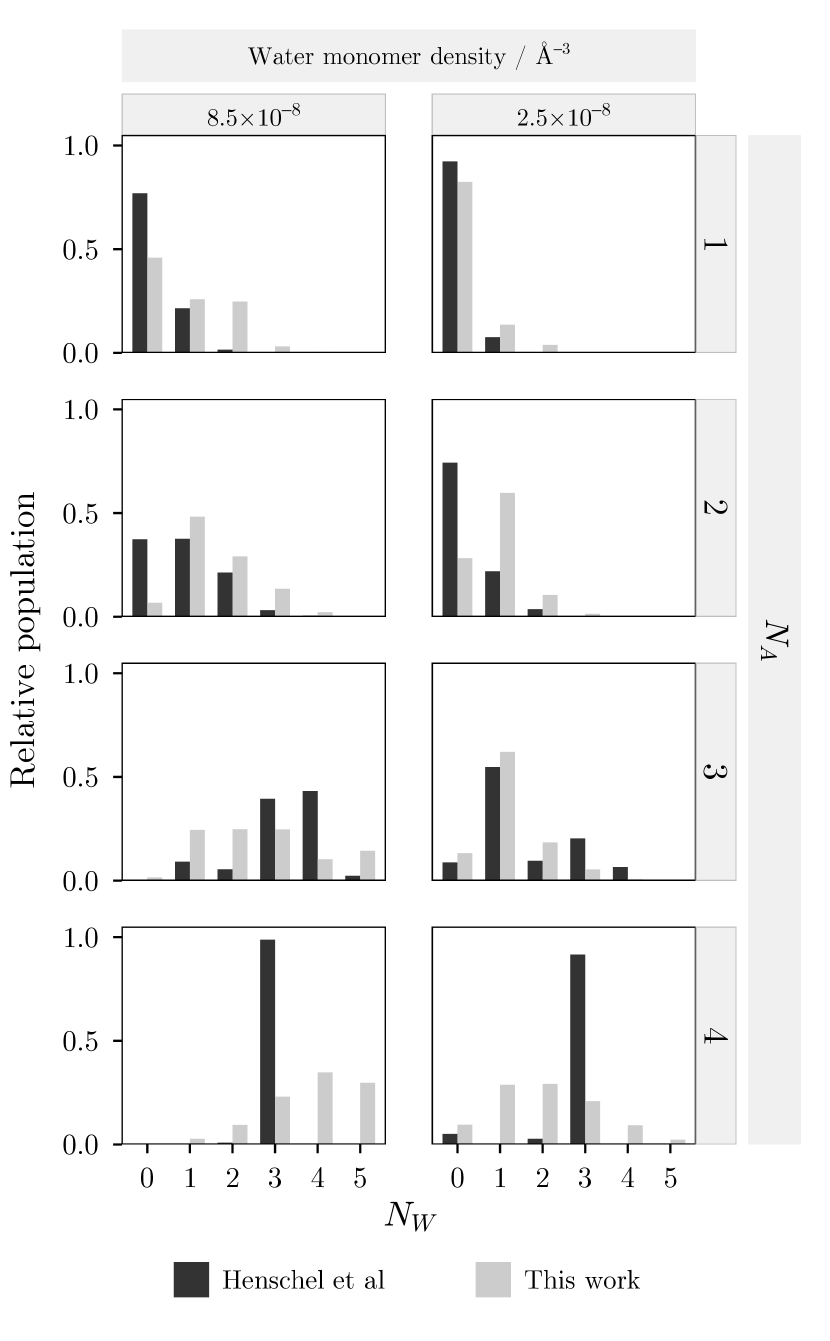
Figure 6: Populations of a variety of clusters of sulphuric acid and water at two water monomer densities, normalised to sum to unity for each value of $N_{A}$ (and hence independent of sulphuric acid monomer density), calculated using our approach (light grey) and taken from Henschel et al. Henschel et al. (2014) (dark grey).

V Conclusions

The key to understanding first order phase transitions in complex gaseous mixtures of precursor molecules is to compute the thermodynamic stability of molecular clusters of various sizes and compositions. Great strides have been made in recent years in extending quantum chemical methods to this area, but an accurate assessment of the entropic contributions to the relevant thermodynamic potentials, for conditions where the clusters are liquid-like, requires an approach that goes beyond a consideration of harmonic fluctuations, currently implying lengthy simulation times or a reduction in the level of treatment from quantum to classical dynamics.

Our approach is to employ a simplified force field for complex molecules fitted to quantum chemical computations Loukonen et al. (2010) and then to use a nonequilibrium classical molecular dynamics procedure to compute the free energy associated with the disassembly of a cluster into its constituent molecules, avoiding a harmonic approximation to the cluster entropy. The separation is brought about by the motion of guide particles, each of which is tethered to one of the molecules in the cluster. The approach offers advantages over typical Monte Carlo methods since the assessment of the properties of a particular cluster is more direct. We do not have to go through a lengthy comparison of ensembles of clusters differing by only one molecule at a time; instead we immediately refer a cluster to a system of separated, though tethered, molecules. The approach is intrinsically a nonequilibrium method, since it involves the mechanical manipulation of a cluster in a finite period of time, driving the system away from equilibrium. We exploit the Jarzynski equality Jarzynski (1997) to extract equilibrium free energy changes from a distribution of nonequilibrium work, while taking care to ensure that the outcomes are independent of the protocol of manipulation.

In this study, we have extended the method to clusters consisting of two molecular species, noting that it could easily be generalised to an arbitrary number. The analysis specifies the way in which the cluster constituents should initially be tethered, and how the free energy of disassembly should be combined with energy and entropy tethering corrections to produce the grand potential that characterises clusters in a binary vapour. When presented as a surface, the grand potential conveys the intuitive idea of a thermodynamic barrier with a critical cluster and preferred path of formation. Our approach provides a new way to construct such a surface in a controlled and well defined fashion, and furthermore, our presentation does not require input of the densities of vapours in equilibrium with the condensed phase, which can complicate the formalism.

We have demonstrated the approach by studying the important binary system of sulphuric acid and water, and have compared our results with those obtained recently using optimised configurations obtained from quantum chemistry together with harmonic fluctuations. The force field employed is simplified, and in particular does not allow proton transfers, but more elaborate models have recently been developed and could be employed in further studies Stinson et al. (2016). We give particular attention to efficiencies available through a suitable performance of the manipulation. Instead of simply pulling the cluster apart with soft harmonic forces, where disassembly proceeds through a sequence of irreversible and violent snapping or tearing events, we prise the molecules apart using guide particles that exert increasingly strong forces while positioned at close range to the cluster. Such a protocol favours molecular removal from the cluster in a manner that is mechanically more reversible, which means that the free energy of disassembly can be obtained from shorter MD simulations. We required 2-3 days of time on the multiprocessor Legion computing facility at UCL to study 46 clusters containing different numbers of the two molecular species.

Our computations do not capture all the dynamic subtleties of a treatment at electronic level, since they are based on a fitted classical force field, but they are very much faster to perform than ab initio methods, and should do better in assessing the entropy of a liquid-like cluster. The comparison between our results and those of Henschel et al. Henschel et al. (2014) is very reasonable and this study will pave the way for further investigations based on improved force fields Stinson et al. (2016) and a wider variety of molecular species Loukonen et al. (2010).

References

- Kashchiev (2000) D. Kashchiev, Nucleation (Butterworth-Heinemann, Oxford, U.K., 2000).
- Ford (2004) I. J. Ford, Proc. Instn Mech. Engnrs Part C: J. Mech. Eng. Sci. 218, 883 (2004).
- Kalikmanov et al. (2008) V. I. Kalikmanov, J. Wölk, and T. Kraska, J. Chem. Phys. 128, 124506 (2008).
- Kalikmanov (2013) V. I. Kalikmanov, Nucleation theory (Springer, Heidelberg, 2013).
- Yasuoka and Matsumoto (1998) K. Yasuoka and M. Matsumoto, J. Chem. Phys. 109, 8463 (1998).
- Kraska (2006) T. Kraska, J. Chem. Phys. 124, 054507 (2006).
- Wedekind et al. (2007) J. Wedekind, J. Wölk, D. Reguera, and R. Strey, J. Chem. Phys. 127, 154515 (2007).
- Tanaka et al. (2011) K. K. Tanaka, H. Tanaka, T. Yamamoto, and K. Kawamura, J. Chem. Phys. 134, 204313 (2011).
- Diemand et al. (2013) J. Diemand, R. Angélil, K. K. Tanaka, and H. Tanaka, J. Chem. Phys. 139, 074309 (2013).
- Angélil et al. (2015) R. Angélil, J. Diemand, K. K. Tanaka, and H. Tanaka, J. Chem. Phys. 143, 064507 (2015).
- Ford (1997) I. J. Ford, Phys. Rev. E 56, 5615 (1997).
- Kurtén and Vehkamäki (2008) T. Kurtén and H. Vehkamäki, Adv. Quantum Chem. 55, 407 (2008).
- Henschel et al. (2014) H. Henschel, J. C. A. Navarro, T. Yli-Juuti, O. Kupiainen-Määttä, T. Olenius, I. K. Ortega, S. L. Clegg, T. Kurtén, I. Riipinen, and H. Vehkamäki, J. Phys. Chem. A 118, 2599 (2014).
- Vehkamäki et al. (2002) H. Vehkamäki, M. Kulmala, I. Napari, K. E. J. Lehtinen, C. Timmreck, M. Noppel, and A. Laaksonen, J. Geophys. Res. Atmos. 107, 4622 (2002).
- Vehkamäki (2006) H. Vehkamäki, Classical nucleation theory in multicomponent systems (Springer, Berlin, 2006).
- Merikanto et al. (2007) J. Merikanto, I. Napari, H. Vehkamäki, T. Anttila, and M. Kulmala, J. Geophys. Res-Atmos. 112 (2007).
- Vehkamäki and Ford (2000) H. Vehkamäki and I. J. Ford, J. Chem. Phys. 112, 4193 (2000).
- Merikanto et al. (2006) J. Merikanto, E. Zapadinsky, and H. Vehkamäki, J. Chem. Phys. 125, 084503 (2006).
- Lee et al. (1973) J. K. Lee, J. Barker, and F. F. Abraham, J. Chem. Phys. 58, 3166 (1973).
- Natarajan et al. (2006) S. Natarajan, S. A. Harris, and I. J. Ford, J. Chem. Phys. 124, 044318 (2006).
- Tang and Ford (2006) H. Y. Tang and I. J. Ford, J. Chem. Phys. 125, 144316 (2006).
- Julin et al. (2008) J. Julin, I. Napari, J. Merikanto, and H. Vehkamäki, J. Chem. Phys. 129, 234506 (2008).
- Tang and Ford (2015) H. Y. Tang and I. J. Ford, Phys. Rev. E 91, 023308 (2015).
- Jarzynski (1997) C. Jarzynski, Phys. Rev. Lett. 78, 2690 (1997).
- Frenkel and Smit (1996) D. Frenkel and B. Smit, Understanding Molecular Simulation: From Algorithms to Applications (Academic Press, 1996).
- Lau et al. (2015) G. V. Lau, P. A. Hunt, E. A. Müller, G. Jackson, and I. J. Ford, J. Chem. Phys. 143, 244709 (2015).
- Kuang et al. (2008) C. Kuang, P. H. McMurry, A. V. McCormick, and F. L. Eisele, J. Geophys. Res. Atmos. 113, 2156 (2008).
- Kirkby et al. (2011) J. Kirkby, J. Curtius, J. Almeida, E. Dunne, J. Duplissy, S. Ehrhart, A. Franchin, S. Gagné, L. Ickes, A. Kürten, et al., Nature 476, 429 (2011).
- Brus et al. (2011) D. Brus, K. Neitola, A.-P. Hyvärinen, T. Petäjä, J. Vanhanen, M. Sipilä, P. Paasonen, M. Kulmala, and H. Lihavainen, Atmos. Chem. Phys. 11, 5277 (2011).
- Loukonen et al. (2010) V. Loukonen, T. Kurtén, I. Ortega, H. Vehkamäki, A. A. Pádua, K. Sellegri, and M. Kulmala, Atmos. Chem. Phys 10, 4961 (2010).
- Yuet and Blankschtein (2010) P. K. Yuet and D. Blankschtein, J. Phys. Chem. B 114, 13786 (2010).
- Todorov et al. (2006) I. T. Todorov, W. Smith, K. Trachenko, and M. T. Dove, J. Materials Chem. 16, 1911 (2006).
- Sloane et al. (2000) N. Sloane, R. Hardin, W. Smith, et al., “Tables of spherical codes,” (2000), Published electronically at http://www.research.att.com/njas/packings.
- Scott (1992) D. W. Scott, Multivariate Density Estimation. Theory, Practice and Visualization (Wiley, New York, 1992).
- Almeida J, Schobesberger S, Kürten A, et al. (2013) Almeida J, Schobesberger S, Kürten A, et al., Nature 502, 359 (2013).
- Stinson et al. (2016) J. L. Stinson, S. M. Kathmann, and I. J. Ford, Mol. Phys. 114, 172 (2016).
- Iland et al. (2007) K. Iland, J. Wölk, and R. Strey, J. Chem. Phys. 127, 154506 (2007).
- Reiss (1950) H. Reiss, J. Chem. Phys. 18, 840 (1950).
- Wilemski and Wyslouzil (1995) G. Wilemski and B. E. Wyslouzil, J. Chem. Phys. 103, 1127 (1995).