$N$-ary Error Correcting Coding Scheme

Abstract

The coding matrix design plays a fundamental role in the prediction performance of the error correcting output codes (ECOC)-based multi-class task. In many-class classification problems, e.g., fine-grained categorization, it is difficult to distinguish subtle between-class differences under existing coding schemes due to a limited choices of coding values. In this paper, we investigate whether one can relax existing binary and ternary code design to $N$-ary code design to achieve better classification performance. In particular, we present a novel $N$-ary coding scheme that decomposes the original multi-class problem into simpler multi-class subproblems, which is similar to applying a divide-and-conquer method. The two main advantages of such a coding scheme are as follows: (i) the ability to construct more discriminative codes and (ii) the flexibility for the user to select the best $N$ for ECOC-based classification. We show empirically that the optimal $N$ (based on classification performance) lies in $[3,10]$ with some trade-off in computational cost. Moreover, we provide theoretical insights on the dependency of the generalization error bound of an $N$-ary ECOC on the average base classifier generalization error and the minimum distance between any two codes constructed. Extensive experimental results on benchmark multi-class datasets show that the proposed coding scheme achieves superior prediction performance over the state-of-the-art coding methods.

I Introduction

Many real-world problems are multi-class in nature. To handle multi-class problems, many approaches have been proposed. One research direction focuses on solving multi-class problems directly. These approaches include decision tree based methods [23, 4, 25, 3, 29, 15, 9]. In particular, decision-tree based algorithms label each leaf of the decision tree with one of the $N_{C}$ classes, and internal nodes can be selected to discriminate between these classes. The performance of decision-tree based algorithms heavily depends on the internal tree structure. Thus, these methods are usually vulnerable to outliers. To achieve better generalization, [29, 15] propose to learn the decision tree structure based on the large margin criterion. However, these algorithms usually involve solving sophisticated optimization problems and their training time increases dramatically with the increase of the number of classes. Contrary to these complicated methods, K-Nearest Neighbour (KNN) [7] is a simple but effective and stable approach to handle multi-class problems. However, KNN is sensitive to noise features and can therefore suffer from the curse-of-dimensionality. Meanwhile, Crammer et al. [8, 17] propose a direct approach for learning multi-class support vector machines (M-SVM) by deriving the generalized notion of margins as well as separating hyperplanes.

Another research direction focuses on the error correcting output codes (ECOC) framework that decomposes a multi-class problem into multiple binary problems so that one reuses the well-studied binary classification algorithms for their simplicity and efficiency. Many ECOC approaches [10, 20, 24, 32, 21, 27, 16] have been proposed in recent years to design a good coding matrix. They fall into two categories: problem-independent and problem-dependent. The challenge with problem-independent codings, such as random ECOC [12], is that they are not designed and optimized for a particular dataset. In fact, there is little guarantee that the created base codes are always discriminative for the multi-class classification task. Therefore, they usually require a large number of base classifiers generated by the pre-designed coding matrix [1]. To overcome this weakness, problem-dependent methods such as discriminant ECOC (DECOC) [22] and node embedding ECOC (ECOCONE) [13] are proposed. Recently, subspace approaches such as subspace ECOC [2] and adaptive ECOC [33] are proposed to further improve the ECOC classification framework. Though all the above-mentioned variations of the ECOC approach endeavor to enhance the ECOC paradigm for classification tasks, their designs are confined to binary $\{-1,1\}$ and ternary codes $\{-1,0,1\}$. Such a code design constraint poses limitations on the error correcting capability of ECOC that relies on the minimum distance, $\Delta_{\min}(M)$, between any distinct pair of rows in the coding matrix $M$. A larger $\Delta_{\min}(M)$ is more likely to rectify the errors committed by individual base classifiers [1].

However, in the more challenging real-world applications, there exists multi-class problems where some of the classes are very similar and difficult to differentiate with each other. For example, in the fine-grained classification [30] unlike basic-level recognition, even humans might have difficulty with some of the fine-grained categorization. One major challenge in fine-grained image classification is to distinguish subtle between-class differences while each class often has large within-class variation in the image level [28]. The existing binary ECOC codes cannot handle this challenge due to limited choices of coding values. It is highly possible that some classes out of multi-class classification problems are assigned with same or similar codes. To address this issue, we investigate whether one can extend the existing binary or ternary coding scheme to an $N$-ary coding scheme to (i) allow users the flexibility to choose $N$ to construct the codes in order to (ii) improve the ECOC classification performance for a given dataset. The main contributions of this paper are as follows.

• We propose a novel $N$-ary coding scheme that achieves a large expected distance between any pair of rows in $M$ at a reasonable $N(>3)$ for a multi-class problem (see Section III). The main idea of our coding scheme is to decompose the original multi-class problem into a series of smaller multi-class subproblems instead of binary classification problems. Suppose that a metaclass is a subset of classes. Also, suppose that all classes are in a one large metaclass. So, in each level, there is a classifier to divide a metaclass into two smaller metaclasses. This coding scheme is like a divide-and-conquer method. The two main advantages of such a coding scheme are as follows: (i) the ability to construct more discriminative codes and (ii) the flexibility for the user to select the best $N$ for ECOC-based classification.

• We provide theoretical insights on the dependency of the generalization error bound of a $N$-ary ECOC on the average base classifier generalization error and the minimum distance between any two constructed codes (see Section V). Furthermore, we conduct a series of empirical analyses to verify the validity of the theorem on the ECOC error bound (see section VI).

• We show empirically that the optimal $N$ (based on classification performance) lies in $[3,10]$ with a slight trade-off in computational cost (see Section VI).

• We show empiricially the superiority of the proposed coding scheme over the state-of-the-art coding methods for multi-class prediction tasks on a set of benchmark datasets (see Section VI).

To the best of our knowledge, there is no previous work that attempts to extend and generalize the coding scheme to $N$-ary codes with $N>3$.

The rest of this paper is organized as follows. Section II reviews the related work. Section III presents the generalization from binary coding to $N$-ary coding. In Section IV,we give the complexity analysis of $N$-ary coding and compare it with other coding schemes with the SVM classifier as a showcase. Section V gives the error bound analysis of $N$-ary coding. Finally, Section VI discusses our empirical studies and Section VII concludes this work.

(a) Multi-class Data

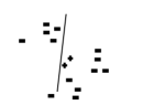
(b) Binary code (e.g., OVA)

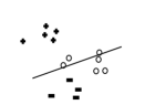
(c) Ternary code (e.g., OVO)

(d) $N$-ary Coding

Figure 1: Fail cases of existing coding scheme: The binary coding scheme sometimes creates non-separate binary classification problems as shown in Figure 1(b). The ternary coding scheme sometimes creates cases where the data from the same class is assigned to different classes as shown in Figure 1(b). $N$-ary coding scheme decomposes the difficult task into some smaller and easier tasks.

II Related Work

Many ECOC approaches [1, 22, 12, 2] have been proposed to design a good coding matrix in recent years. Most of them fall into the following two categories. The first one is problem-independent coding, such as OVO, OVA, random dense ECOC, and random sparse ECOC [12]. However, the coding matrix design is not optimized for the training dataset or the instance labels. Therefore, these approaches usually require a large number of base classifiers generated by the pre-designed coding matrix. For example, the random dense ECOC coding approach aims to construct the ECOC matrix $M\in\{-1,1\}^{N_{C}\times N_{L}}$ where $N_{C}$ is the number of classes, $N_{L}$ is the code length, and its elements are randomly chosen as either 1 or -1 [11]. [1] extends this binary coding scheme to ternary coding by using a coding matrix $M\in\{-1,0,1\}^{N_{C}\times N_{L}}$ where the classes corresponding to 0 are not considered in the learning process. Allwein et al. [1] suggest that dense and sparse random ECOC approaches require only $10\log_{2}(N_{C})$ and $15\log_{2}(N_{C})$ base classifiers, respectively, to achieve optimal results. However, a random ECOC coding approach cannot guarantee that the created base codes are always discriminative for the multi-class classification task. Therefore, it is possible that either some base classifiers that are redundant for the prediction exist or badly designed base classifiers are constructed.

To overcome this problem, some problem-dependent methods have been proposed. In particular, the coding matrix is learned by taking the instances as well as labels into consideration. For instance, discriminant ECOC (DECOC) [22] embeds a binary decision tree into the ternary codes. Its key idea is to find the most discriminative hierarchical partition of the classes which maximizes the quadratic mutual information between the data subsets and the class labels created for each subset. As a result, DECOC needs exactly $N_{C}-1$ base classifiers which significantly accelerate the testing process without sacrificing performance. However, this decision tree based method has one major drawback: if the parent node misclassifies an instance, the mistake will be propagated to all the subsequent child nodes.

To address this weakness, Escalera et al. [13] proposed to optimize node embedding for ECOC, called ECOCONE. For this approach, one initializes a problem-independent ECOC matrix (usually OVA) and iteratively adds the base classifiers that discriminate the most confusing pairs of classes into the previous ECOC ensemble to improve performance. However, ECOCONE suffers from three major limitations. Firstly, its performance relies on the initial coding matrix. If the initial coding matrix fails to perform well, the final results of ECOCONE are usually unsatisfactory. Secondly, its improvement is usually hindered if it fails to discriminate the most confusing pairs. Lastly, similar to DECOC, the training process is also time-consuming.

In addition to the above problem-dependent ECOC methods, Rocha et al. [24] considers the correlation and joint probability of base binary classifiers to reduce the number of base classifiers without sacrificing accuracy in the ECOC code design. More recently, Zhao et al. [32] proposed to impose the sparsity criterion into output code learning. It is shown to have much better performance and scalability to large scale classification problems compared to traditional methods like OVA. However, it involves a series of complex optimizations to solve the proposed model with integer constraints in learning the ECOC coding matrix.

Different from the aforementioned methods, some subspace approaches have been developed. For example, subspace ECOC [2] is based on using different feature subsets for learning each base classifier to improve independence among classifiers. Adaptive ECOC [33] reformulates the ECOC models into multi-task learning where the subspace for data and base classifiers are learned.

Due to the favorable properties and promising performance of ECOC approaches for the classification task, they have been applied to real-world classification applications such as face verification [18], ECG beats classification [27], and even beyond multi-class problems, such as feature extraction [34] and fast similarity search [31].

Though all the above-mentioned variations of the ECOC approach endeavor to enhance the ECOC paradigm for the classification task, their designs are still based on either binary or ternary codes which lack some desirable properties available in their generalized form.

III From A Binary to $N$-ary Coding Matrix

In this section, we discuss necessities and advantages of $N$-ary coding scheme from aspects of column correlation of coding matrix and separation between codewords of different classes.

Existing ECOC algorithms constrain the coding values either in $\{-1,1\}$ or $\{-1,0,1\}$. A lot of studies show that when there are sufficient classifiers, ECOC can reach stable and reasonable performance [24, 11]. Nevertheless, binary and ternary codes can generate at most $2^{N_{C}}$ and $3^{N_{C}}$ binary classifiers, where $N_{C}$ denotes the number of classes. On the other hand, due to limited choices of coding values, existing codes tend to create correlated and redundant classifiers and make them less effective “voters”. Moreover, some studies show that binary and ternary codes usually require only $10\log_{2}(N_{C})$ and $15\log_{2}(N_{C})$ base classifiers, respectively, to achieve optimal results [1, 12]. Furthermore, when the original multi-class problem is difficult, the existing coding schemes cannot handle well. For example, as shown in Figure 1(b), the binary codes like OVA may create difficult base binary classification tasks. Ternary codes may cause cases where the test data from the same class is assigned to different classes.

TABLE I: An example of $N$-ary coding matrix $M$ with $N=4$ and $N_{L}=6$.

	$M_{1}$	$M_{2}$	$M_{3}$	$M_{4}$	$M_{5}$	$M_{6}$
$C_{1}$	1	1	2	4	1	1
$C_{2}$	2	1	1	3	2	1
$C_{3}$	3	2	1	2	3	1
$C_{4}$	4	3	1	1	4	2
$C_{5}$	4	3	2	2	4	3
$C_{6}$	4	3	3	3	3	4
$C_{7}$	3	4	4	4	2	4

To address these issues, we extend the binary or ternary codes to $N$-ary codes. One example of the $N$-ary coding matrix to represent seven classes is shown in Table I. Unlike the existing ECOC framework, a row of coding matrix $M$ represents the code of each class and the code consists of $N_{L}$ numbers in $\{1\cdots N\}$, where $N>3$; while a column $M_{s}$ of $M$ represents the $N$ partitions of classes to be considered. To be specific, the $N$-ary ECOC approach consists of four main steps:

1. Generate an $N$-ary matrix $M$ by uniformly random sampling from a range $\{1..N\}$ (e.g., Table I).

2. For each of the $N_{L}$ matrix columns, partition original training data into $N$ groups based on the new class assignments and build an $N$-class classifier.

3. Given a test example ${\mathbf{x}}_{t}$, use the $N_{L}$ classifiers to output $N_{L}$ predicted labels for the testing output code (e.g., $f({\mathbf{x}}_{t})=[4,3,1,2,4,2]$).

4. Final label prediction $y_{t}$ for ${\mathbf{x}}_{t}$ is the nearest class based on minimum distance between the training and the testing output codes (e.g., $y_{t}=\arg\min_{i}d(f({\mathbf{x}}_{t}),C_{i})=4$ ).

One notes that $N$-ary ECOC randomly breaks a large multi-class problem into a number of smaller multi-class subproblems. These subproblems are more complicated than binary problems and they incur additional computational cost. Hence, there is a trade-off between error correcting capability and computational cost. Fortunately, our empirical studies indicate that $N$ does not need to be too large to achieve good classification performance.

III-A Column Correlations of Coding Matrix

Figure 2: Column Correlation Comparison ( PCC v.s. $N_{L}$ )

In traditional ECOC, it suggests longer codes, i.e., $N_{L}$ is larger, however more binary base classifiers are likely to be more correlated. Thus, more base classifiers created by binary or ternary codes are not effective for final multi-class classification. To illustrate the advantage of $N$-ary coding scheme in creating uncorrelated codes for base classifications, we conduct an experiment to investigate the column correlations of matrix $M$. The results are shown in the Figure 2. In the experiment, we set $N_{C}=20,N=5,$ and $N_{L}$ varies in $[10,80]$, and use Pearson’s correlation (PCC) which is a normalized correlation measure that eliminates the scaling effect of the codes. From Figure 2, we observe that $N$-ary coding scheme achieves lower correlations for columns of coding matrix compared to conventional ternary ECOC. Especially, when the number of tasks is small, the correlations over the created tasks for ECOC is higher than that of the $N$-ary ECOC. Therefore, an $N$-ary coding scheme not only provides more flexibility in creating a coding matrix, but also generates codes that are less correlated and less redundant, compared to traditional ECOC coding schemes.

III-B Separation Between Codewords of Different Classes

Apart from the column correlation, the row separation is another important measure to evaluate the error correcting ability of the coding matrix $M$ [11, 1]. The codes for different classes are expected to be as dissimilar as possible. If codes (rows) for different classes are similar, it is easier to commit errors. Thus, the capability of error correction relies on the minimum distance, $\Delta_{\min}(M)$ or expected $\Delta(M)$ for any distinct pair of rows in the coding matrix $M\in\{-1,0,1\}^{N_{C}\times N_{L}}$ where $N_{C}$ is the number of classes, and $N_{L}$ is the code length. Both the absolute distance and the Hamming distance can serve as the measure of row separation. The key difference between these two distances is that Hamming distance measures a scale-invariant difference. Specifically, the Hamming distance only cares about the number of different elements. It ignores the scale of the difference.

Hamming Distance: One can use the generalized Hamming distance to calculate the $\Delta^{Ham}(M)$ for the existing coding schemes, which is defined as follows,

Definition 1 (Generalized Hamming Distance).

Let $M(r_{1},:),M(r_{2},:)$ denote row $r_{1},r_{2}$ coding vectors in coding matrix $M$ with length $N_{L}$, respectively. Then the generalized hamming distance can be expressed as

$$\Delta^{Ham}(M(r_{1},:),M(r_{2},:))=$$

$$\!\!\!\!\sum_{s=1}^{N_{L}}\left\{\begin{array}[]{cl}\!\!\!\!\!\!\!\!\!0\!\!&\!\!\textrm{if}~{}M(r_{1},s)\!=\!M(r_{2},s)\wedge M(r_{1},s)\neq 0\wedge M(r_{2},s)\neq 0\\ \!\!\!\!\!\!\!\!\!1\!\!&\!\!\textrm{if}~{}M(r_{1},s)\!\neq\!M(r_{2},s)\wedge M(r_{1},s)\neq 0\wedge M(r_{2},s)\neq 0\\ \!\!\!\!0.5&\!\!\textrm{if}~{}M(r_{1},s)\!=\!0\vee M(r_{2},s)\!=\!0.\\ \end{array}\right.$$ (4)

For the OVA coding, every two rows have exactly two entries with opposite signs, $\Delta_{min}^{Ham(OVA)}(M)=2$. For the OVO coding, every two rows have exactly one entry with opposite signs, $\Delta_{min}^{Ham(OVO)}(M)=\left(\left(\begin{array}[]{c}\!\!\!\!N_{C}\!\!\!\!\\ \!\!\!\!2\!\!\!\!\end{array}\right)-1\right)/2+1$, where $N_{C}$ is the number of classes. Moreover, for a random coding matrix with its entries uniformly chosen, the expected value of any two different class codes is $\Delta^{Ham(RAND)}(M)$ is $N_{L}/2$, where $N_{L}$ is the code length. A larger $\Delta^{Ham(RAND)}(M)$ is more likely to rectify the errors committed by individual base classifiers. Therefore, when $N_{L}\gg N_{C}$, a random ECOC is expected to be more robust and rectify more errors than the OVO and OVA approaches  [1]. However, the choice of only either binary or ternary codes hinders the construction of longer and more discriminative codes. For example, binary codes can only construct codes of length $N_{L}\leq 2^{N_{C}}$. Moreover, they lead to many redundant base learners [12]. In contrast, for $N$-ary ECOC, the expected value of $\Delta^{Ham(N)}(M)$ is $N_{L}(1-\frac{1}{N})$ (see Lemma 1 for proof). $\Delta^{Ham(N)}(M)$ is expected to be larger than $\Delta^{Ham(RAND)}(M)$ when $N\geq 3$.

TABLE II: Comparison of Distance of Different Codes.

Coding	Generalized	Absolute
Schemes	Hamming Distance	Distance
OVA	$2$	$4$
OVO	$\left(\left(\begin{array}[]{c}\!\!\!\!N_{C}\!\!\!\!\\ \!\!\!\!2\!\!\!\!\end{array}\right)-1\right)/2+1$	$2N_{C}-2$
ECOC	$N_{L}/2$	$N_{L}$
$N$-ary ECOC	$N_{L}(1-1/N)$	$N_{L}(N^{2}-1)/3N$

Lemma 1.

The expected Hamming distance for any two distinct rows in a random $N$-ary coding matrix $M\in\{1,2,\cdots,N\}^{N_{C}\times N_{L}}$ is

$$\Delta^{Ham(N)}(M)=N_{L}(1-\frac{1}{N}).\vspace{-3mm}$$ (5)

Proof.

Given a random matrix $M$ with components chosen uniformly over $\{1,2,\cdots,N\}$, for any distinct pair of entries in column $s$, i.e., $M(r_{i},s)$ and $M(r_{j},s)$, the probability of $M(r_{i},s)=M(r_{j},s)$ is $\frac{1}{N}$. Then the probability of $M(r_{i},s)\neq M(r_{j},s)$ is $1-\frac{1}{N}$.

Therefore, according to Definition 1, the expected Hamming distance for $M$ can be computed as follows,

$$\Delta^{Ham(N)}(M) = N_{L}\left(1\times(1-\frac{1}{N})+0\times\frac{1}{N}\right)$$

$$= N_{L}(1-\frac{1}{N}).$$

∎

Absolute Distance: Different from the Hamming distance, the absolute distance measures the difference scales. Thus, for a fair comparison, we assume that coding values are in the same scale for the absolute distance analysis. The definition of absolute distance is given as follows,

Definition 2 (Absolute Distance).

Let $M(r_{1},:)$ and $M(r_{2},:)$ denote row $r_{1}$ and $r_{2}$ coding vectors in coding matrix $M$ with length $N_{L}$, respectively. Then the absolute distance can be expressed as

$$\Delta^{abs}(M(r_{1},:),M(r_{2},:))=\sum_{s=1}^{N_{L}}|M(r_{1},s)-M(r_{2},s)|.$$

For the convenience of analysis, we first give the expected absolute distance for $N$-ary coding matrix in Lemma 2.

Lemma 2.

The expected absolute distance for any two distinct rows in a random $N$-ary coding matrix $M\in\{1,2,\cdots,N\}^{N_{C}\times N_{L}}$ is

$$\Delta^{abs(N)}(M)=N_{L}\frac{(N^{2}-1)}{3N}.$$ (6)

Proof.

Given a random matrix $M$ with components chosen uniformly over $\{1,2,\cdots,N\}$, for any distinct pair of entries in column $s$, i.e., $M(r_{i},s),M(r_{j},s)$, we denote the corresponding expected absolute distance as $\Delta^{abs(N)}(M(:,s))={\mathbb{E}}~{}{d_{ij}}={\mathbb{E}}~{}|M(r_{i},s)-M(r_{j},s)|$.

It can be calculated by averaging all the possible pairwise distances $d_{ij}$ for $i,j\in\{1,2,\cdots,N\}$. Since the two numbers $r_{i},r_{j}$ are chosen randomly from $\{1,...,N\}$, $\Delta^{N}(M)$ can be expressed as follows:

$$\Delta^{abs(N)}(M(:,s)) = \frac{1}{N^{2}}\sum_{i,j=1}^{N}d_{ij}$$ (7)

$$= \frac{1}{N^{2}}\sum_{i,j=1}^{N}|M(r_{i},s)-M(r_{j},s)|$$

TABLE III: All Possible Choices of $d_{ij}$.

$d_{ij}$	$r_{j}=1$	$r_{j}=2$	$\cdots$	$r_{j}=N$
$r_{i}=1$	0	1	$\cdots$	N-1
$r_{i}=2$	1	0	$\cdots$	$\vdots$
$\vdots$	$\vdots$	$\vdots$	0	1
$r_{i}=N$	N-1	$\cdots$	1	0

First, we define the sequence $a_{n}$ as follows:

$$a_{n}=(1+2+\cdots+n)=\frac{n(n+1)}{2}.$$ (8)

Table III gives all the possible choices of $d_{ij}$. Thus the calculation of $\Delta^{N}(M)$ is equal to taking the average of all the entries in Table III, which can be expressed as follows:

$$\Delta^{abs(N)}(M(:,s))\!\!\!\!\!\! = \!\!\!\!\!\!\frac{2}{N^{2}}(a_{1}+a_{2}+\cdots+a_{N-1})$$

$$= \!\!\!\!\!\!\frac{1}{N^{2}}(1\times 2+2\times 3+\cdots+(N-1)N)$$

$$= \!\!\!\!\!\!\frac{1}{N^{2}}\sum_{n=1}^{N}(n^{2}-n)$$

$$= \!\!\!\!\!\!\frac{1}{N^{2}}\left(\sum_{n=1}^{N}n^{2}-\sum_{n=1}^{N}n\right)$$

$$= \!\!\!\!\!\!\frac{1}{N^{2}}\left(\frac{N(N+1)(2N+1)}{6}-\frac{N(N+1)}{2}\right)$$

$$= \!\!\!\!\!\!\frac{N^{2}-1}{3N},$$

where (III-B) comes from the symmetry of $d_{ij}$. Then

$$\Delta^{abs(N)}(M)=\sum_{s=1}^{N_{L}}\Delta^{abs(N)}(M(:,s))=N_{L}\frac{(N^{2}-1)}{3N}.$$

∎

For the OVA coding scheme, every two rows have exactly two entries with opposite signs, the minimum absolute distance $\Delta_{min}^{abs(OVA)}(M)=4$; while for the OVO coding scheme, every two rows have exactly one entry with opposite signs and only $2N_{C}-4$ entries with a difference of exactly one, $\Delta_{min}^{abs(OVO)}(M)=2N_{C}-2$. For binary random codes, the expected absolute distance between any two different rows is $\Delta^{abs(RAND)}(M)=N_{L}$. Thus, when $N$ is large, $\Delta^{abs(N)}(M)$ is much larger than $\Delta^{abs(RAND)}(M)$, and $N$-ary coding is expected to be better.

The Hamming and absolute distance comparisons for different codes are summarized in the Table II. We can see that $N$-ary coding scheme has an advantage in creating more discriminative codes with larger distances for different classes in both two distance measures. This advantage is very important to analyze the generalization error analysis of $N$-ary ECOC.

IV Complexity Comparison

As discussed in Section III, $N$-ary codes have a better error correcting capability than the traditional random codes when $N$ is larger than 3. However, one notes that the base classifier of each column is no longer solving a binary problem. Instead, we randomly break a large multi-class problem into a number of smaller multi-class subproblems. These subproblems are more complicated than binary problems and they incur additional computational cost. Hence, there is a trade-off between the error correcting capability and computational cost.

If the complexity of the algorithm employed to learn the small-size multi-class base problem is $\mathcal{O}(g(N,N_{tr},d))$ with $N$ classes, $N_{tr}$ training examples, $d$ predictive features and $g(N,N_{tr},d)$ is the complexity function w.r.t $N$, $N_{tr}$, $d$, then the computational complexity of $N$-ary codes is $\mathcal{O}(N_{L}g(N,N_{tr},D))$ for codes of length $N_{L}$.

Taking SVM as the base learner for example, one can learn each binary classification task created by binary ECOC codes with training complexity of $\mathcal{O}(N_{tr}^{3})$ for traditional SVM solvers that build on the quadratic programming (QP) problems. However, a major stumbling block for these traditional methods is in scaling up these QP s to large data sets, such as those commonly encountered in data mining applications. Thus, some state-of-the-art SVM implementations, e.g., LIBSVM [6], Core Vector Machines [26], have been proposed to reduce training time complexity from $\mathcal{O}(N_{tr}^{3})$ to $\mathcal{O}(N_{tr}^{2})$ and $\mathcal{O}(N_{tr})$, respectively. Nevertheless, how to efficiently train SVM is not the focus of our paper. For the convenience of complexity analysis, we use the time complexity of the traditional SVM solvers as the complexity of the base learners. Then, the complexity of binary ECOC codes is $\mathcal{O}(N_{L}N_{tr}^{3})$. Different from ECOC in the ensemble manner, one can directly address the multi-class problem in one single optimization process, e.g., multi-class SVM [8]. This kind of model combines multiple binary-class optimization problems into one single objective function and simultaneously achieves the classification of multiple classes. In this way, the correlations across multiple binary classification tasks are captured in the learning model. The resulting QP optimization requires a complexity of $\mathcal{O}((N_{C}N_{tr})^{3})$. However, it causes high computational complexity for a relatively large number of classes. In contrast, $N$-ary codes are in the complexity of $\mathcal{O}(N_{L}(NN_{tr})^{3})$, where $N<N_{C}$. In this case, it achieves better trade-off between the error correcting capability and computational cost, especially for large class size $N_{C}$.

We summarize the time complexity of different codes in Table IV. In Section VI-A4, our empirical studies indicate that $N$ does not need to be too large to achieve optimal classification performance.

TABLE IV: Complexity Analysis

Classifier	SVM
Binary ECOC	$\mathcal{O}(N_{L}N_{tr}^{3})$
Direct Multi-Class	$\mathcal{O}((N_{C}N_{tr})^{3})$
$N$-ary ECOC	$\mathcal{O}(N_{L}(NN_{tr})^{3})$

V Generalization Analysis of $N$-ary ECOC.

In Section V-A, we study the error correcting ability of an $N$-ary code. In Section V-B, we derive the generalization error bound for $N$-ary ECOC independent of the base classifier.

V-A Analysis of Error Correcting on $N$-ary Codes

To study the error correcting ability of $N$-ary codes, we first define the distance between the codes in any distinct pair of rows, $M(r_{i})$ and $M(r_{j})$, in an $N$-ary coding matrix $M$ as $\Delta^{N}(M(r_{i}),M(r_{j}))$. It is the sum of the $N_{L}$ distances between two entries, $M(r_{i},s)$ and $M(r_{j},s)$ in the same column $s$ at two different rows, $r_{i}$ and $r_{j}$, i.e., $\Delta^{N}(M(r_{i}),M(r_{j}))=\sum_{s=1}^{N_{L}}\Delta^{N}(M(r_{i},s),M(r_{j},s)).$ We further define $\rho=\min_{r_{i}\neq r_{j}}{\Delta^{N}(M(r_{i}),M(r_{j}))}$ as the minimum distance between any two rows in $M$.

Proposition 3.

Given an $N$-ary coding matrix $M$ and a vector of predicted labels $f({\mathbf{x}})=[f_{1}({\mathbf{x}})),\cdots,f_{N_{L}}({\mathbf{x}}))]$ by $N_{L}$ base classifiers for a test instance ${\mathbf{x}}$. If ${\mathbf{x}}$ is misclassified by the $N$-ary ECOC decoding, then the distance between the correct label in $M(y)$ and $f({\mathbf{x}})$ is greater than one half of $\rho$, i.e.,

$$\Delta^{N}(M(y),f({\mathbf{x}}))\geq\frac{1}{2}\rho.$$ (10)

Proof.

Suppose that the distance-based decoding incorrectly classifies a test instance ${\mathbf{x}}$ with known label $y$. In other words, there exists a label $r\neq y$ for which

$$\Delta^{N}(M(y),f({\mathbf{x}}))\geq\Delta^{N}(M(r),f({\mathbf{x}})).$$

Here, $\Delta^{N}(M(y),f({\mathbf{x}}))$ and $\Delta^{N}(M(r),f({\mathbf{x}}))$ can be expanded as the element-wise summation. Then, we have

$$~{}~{}\sum_{s=1}^{N_{L}}\Delta^{N}(M(y,s),f_{s}({\mathbf{x}}))\geq\sum_{s=1}^{N_{L}}\Delta^{N}(M(r,s),f_{s}({\mathbf{x}})).$$ (11)

Based on the above inequality, we obtain:

$$\Delta^{N}(M(y),f({\mathbf{x}}))$$

$$\!\!\!\!\!= \!\!\!\!\!\frac{1}{2}\sum_{s=1}^{N_{L}}\left\{\Delta^{N}(M(y,s),f_{s}({\mathbf{x}}))\!+\!\Delta^{N}(M(y,s),f_{s}({\mathbf{x}}))\right\}$$

$$\!\!\!\!\geq \!\!\!\!\!\!\frac{1}{2}\sum_{s=1}^{N_{L}}\{\Delta^{N}(M(y,s),f_{s}({\mathbf{x}}))\!+\!\Delta^{N}(M(r,s),f_{s}({\mathbf{x}}))\}$$ (12)

$$\!\!\!\!\geq \!\!\!\!\!\!\frac{1}{2}\sum_{s=1}^{N_{L}}\{\Delta^{N}(M(y,s),M(r,s))\}\!\!$$ (13)

$$\!\!\!\!= \!\!\!\!\!\!\frac{1}{2}{\Delta^{N}(M(r),M(y))}$$

$$\!\!\!\!\geq \!\!\!\!\!\!\frac{1}{2}\rho,$$

where Inequality (12) uses Inequality (11) and Inequality (13) follows from the triangle inequality.∎

Remark 1.

From Proposition 3, one notes that a mistake on a test instance $({\mathbf{x}},y)$ implies that $\Delta^{N}(M(y),f({\mathbf{x}}))\geq\frac{1}{2}\rho$. In other words, the prediction codes are not required to be exactly the same as the ground-truth codes for all the base classifications. As long as the distance is no larger than $\frac{1}{2}\rho$, $N$-ary ECOC can rectify the error committed by some base classifiers, and is still able to make an accurate prediction. This error correcting ability is very important especially when the labeled data is insufficient. Moreover, a larger minimum distance, i.e., $\rho$, leads to a stronger capability of error correcting. Note that this proposition holds for all the distance measures and traditional ECOC schemes due to the fact that only the triangle inequality is required in the proof.

V-B Generalization Error of $N$-ary ECOC.

The next result provides a generalization error bound for any type of base classifier, such as the SVM classifier and decision tree, used in the $N$-nary ECOC classification.

Theorem 4 ($N$-ary ECOC Error Bound).

Given $N_{L}$ base classifiers, $f_{1},\cdots,f_{N_{L}}$, trained on $N_{L}$ subsets $\{({\mathbf{x}}_{i},M(y_{i},s))_{i=1,\cdots,N_{tr}}\}_{s=1,\cdots,N_{L}}$ of the dataset with $N_{tr}$ instances for coding matrix $M\in\{1,2,\cdots,N\}^{N_{C}\times N_{L}}$. The generalized error rate for the $N$-ary ECOC approach using distance-based decoding is upper bounded by

$$\frac{2N_{L}\bar{B}}{\rho},$$ (14)

where $\bar{B}=\frac{1}{N_{L}}\sum_{s=1}^{N_{L}}B_{s}$ and $B_{s}$ is the upper bound of the distance-based loss for the $s^{th}$ base classifier.

Proof.

According to Proposition 3, for any misclassified data instance, the distance between its incorrect label vector $f({\mathbf{x}})$ and the true label vector $M(y)$ should satisfy the minimal distance $\frac{\rho}{2}$, i.e., $\Delta^{N}(M(y),f({\mathbf{x}}))=\sum_{s=1}^{N_{L}}\Delta^{N}(M(y,s),f_{s}({\mathbf{x}}))\geq\frac{\rho}{2}.$

Let $a$ be the number of incorrect label predictions for a set of test instances of size $N_{te}$. One obtains

$$a\frac{\rho}{2}\leq\sum^{N_{te}}_{i=1}\sum^{N_{L}}_{s=1}\Delta^{N}(M(y_{i},s),f({\mathbf{x}}_{i})).$$ (15)

Then,

$$a\leq\frac{2N_{te}\sum^{N_{L}}_{s=1}B_{s}}{\rho}=\frac{2N_{te}N_{L}\bar{B}}{\rho},$$ (16)

where $\bar{B}=\frac{1}{N_{L}}\sum_{s=1}^{N_{L}}B_{s}$.

Hence, the testing error rate is bounded by $\frac{2{N_{L}}\bar{B}}{\rho}$. ∎

Remark 2.

From Theorem 4, one notes that for the fixed $N_{L}$, the generalization error bound of the $N$-ary ECOC depends on the two following factors:

1. The averaged loss $\bar{B}$ for all the base classifiers. In practice, some base tasks may be badly designed due to the randomness. As long as the averaged loss $\bar{B}$ over all the tasks is small, the resulting ensemble classifier is still able to make a precise prediction.

2. The minimum distance $\rho$ for coding matrix $M$. As we discussed in Proposition 3, the larger $\rho$, the stronger capability of error correcting $N$-ary code has.

Both two factors are affected by the choice of $N$. In particular, $\bar{B}$ increases as $N$ increases since the base classification tasks become more difficult. On the other hand, from experimental results in Figure 3(b), it is observed that $\rho$ becomes larger when $N$ increases. Therefore, there is a tradeoff between these two factors.

VI Experimental Results

We present experimental results on 11 well-known UCI multi-class datasets from a wide range of application domains. The statistics of these datasets are summarized in Table V. The parameter $N$ is chosen by cross-validation procedure. With the tuned parameters, all methods are run ten realizations. Each has different random splittings with fixed training and testing size as given in Table V. Our experimental results focus on the comparison of different encoding schemes rather than decoding schemes. Therefore, we fix generalized hamming distance as the decoding strategy for all the coding designs for a fair comparison.

TABLE V: Summary of the datasets used in the experiments.

Dataset	#Train	#Test	#Features	#Classes
Pendigits	3498	7494	16	10
Vowel	462	528	10	10
News20	3993	15935	62061	20
Letters	5000	15000	16	26
Auslan	1000	1565	128	95
Sector	3207	6412	55197	105
Aloi	50000	58000	128	1000
Glass	100	114	9	10
Satimage	3435	3000	36	7
Usps	4298	5000	256	10
Segment	1310	1000	19	7

To investigate the effectiveness of the proposed $N$-ary coding scheme, we compare it with problem-independent coding schemes including OVO, OVA, and random ECOC as well as the state-of-art problem-dependent methods such as ECOCONE and DECOC. For the random ECOC encoding scheme, or ECOC in short, and the $N$-ary ECOC strategy, we select the matrix with the largest minimum absolute distance from 1000 randomly generated matrices.

For the problem-dependent approach DECOC, the length of the ECOC codes is exactly $N_{C}-1$ [22]. For the ECOCONE, we initialize the ECOC matrix with OVA matrix [13]. The length of the ECOC code is also learned during the training step. We use the ECOC library [14] for the implementation of all these baseline methods. To ensure a fair comparison and easy replication of results, the base learners decision tree CART [5] and linear SVM are implemented with the CART decision tree MATLAB toolbox and the LIBSVM [6] with the linear kernel in default settings, respectively.

VI-A Error Bound Analysis on $N$-ary ECOC.

In the bound analysis, we choose hamming distance 1 to measure the row separation as a showcase. According to Theorem 4, the generalization error bound depends on the minimum distance $\rho$ between any two distinct rows in the $N$-ary coding matrix $M$ as well as the average loss of base classifiers $\bar{B}$. In particular, the expected value of $\Delta^{N}(M)$ scales with $O(N)$.

In this subsection, we investigate the effect of the number of classes $N$ using the Pendigits dataset with CART as the base classifier to illustrate the following aspects: (i) $\Delta^{N}(M)$ between any two distinct rows of codes (see Figure 3(a) ), (ii) $\rho$ (see Figure 3(b)), (iii) $\frac{\bar{B}}{\rho}$ (see Figure  3(c)), and (iv) the classification performance (see Figure 4). The empirical results corroborate the proposed error bounds in Theorem 4.

(a) Average $\Delta^{N}(M)$ v.s. $N$.

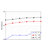
(b) $\rho$ v.s. $N$.

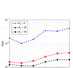
(c) $\frac{\bar{B}}{\rho}$ v.s. $N$.

Figure 3: Experimental results to study error bound (Theorem 4) w.r.t. $N$.

VI-A1 Average distance $\Delta^{N}(M)$ v.s. $N$.

Recall that the hamming distance for different coding matrices discussed in Section III are: $\Delta^{N}(M)=N_{L}(1-\frac{1}{N})$, $\Delta^{rand}(M)=N_{L}/2$, $\Delta_{\min}^{ova}(M)=2$ and $\Delta_{\min}^{ovo}(M)=\left(\left(\begin{array}[]{c}\!\!\!\!N_{C}\!\!\!\!\\ \!\!\!\!2\!\!\!\!\end{array}\right)-1\right)/2+1$.

From Figure 3(a), we observe that the empirical average hamming distances of the constructed $N$-ary coding matrices for random $N$-ary schemes are close to $N_{L}(1-\frac{1}{N})$. Furthermore, when there are 45 base classifiers, the average distance for $N$-ary ECOC is larger than 30, which is larger than that of the binary random codes with an average absolute distance of 22.5. Moreover, a higher $N$ leads to a larger average distance. Comparing Figure 3(a) and Figure 3(b) , the large average distance $\Delta^{N}(M)$ also correlates with the large minimum distance $\rho$.

VI-A2 Minimum distance $\rho$ v.s. $N$.

For the Pendigits dataset with 10 classes, $\rho$ for OVA and OVO are 4 and 18, respectively. From Figure 3(b), we observe that with a fixed number of base classifiers, $\rho$ increases with the number of multi-class subproblems of class-size $N$, meanwhile $\rho$ also increases with respect to the code length $N_{L}$. Furthermore, in comparison to the other coding schemes, our proposed method usually creates a coding matrix with a large $\rho$. For example, in Figure 3(b), one observes that when there are 25 and 45 base classifiers, the corresponding $\rho$ for binary random codes are 0. On the other hand, $N$-ary ECOC, given a sufficiently large $N$, creates an $N$-ary coding matrix with $\rho$ to be larger than 10 and 20, respectively. Although $N$-ary ECOC creates an $N$-ary coding matrix with a large $\rho$ when $N$ is larger, in real-world applications, it is preferred that $N$ is not too large to ensure reasonable computational cost and difficulty of subproblems. In short, $N$-ary ECOC provides a better alternative to creating a coding matrix with a large class separation compared to traditional coding schemes.

VI-A3 Ratio $\bar{B}/\rho$ v.s. $N$.

Both $\bar{B}$ and $\rho$ are dependent on $N$. Moreover, from the generalization error bound, we observe that $\bar{B}/\rho$ directly affects classification performance. Hence, this ratio, which bounds the classification error, requires further investigation. Figure 3(c) shows that when $N=4$, the ratio $\bar{B}/\rho$ is lowest. This observation suggests that the more the row and column separation of the coding matrix, the stronger the capability of error correction [11]. Therefore, $N$-ary ECOC is a better way to creating the coding matrix with large separation among the classes as well as more diversity, compared to the binary and ternary coding schemes. One notes that $\bar{B}/\rho$ starts to increase when $N\geq 5$. This means that the increase of the average base classifier loss $\bar{B}$ overwhelms the increase in $\rho$. The reason for this phenomena is the increase in difficulty of the subproblem classification with more classes.

VI-A4 Classification Accuracy v.s. $N$.

Next, we study the impact of $N$ on the multi-class classification accuracy. We use datasets Pendigits, Letters, Sectors, Aloi with 10 classes, 26 classes, 105 classes, 1000 classes respectively as showcase. In order to a obtain meaningful analysis, we choose a suitable classifier for different datasets. In particular, we apply the CART to datasets Pendigits, Letters and Aloi and linear SVM to Sectors. One observes from Figure 4 that the $N$-ary ECOC achieves competitive prediction performance when $3\leq N\leq 10$. However, given sufficient base learners, the classification error starts increasing when $N$ is large (e.g. $N>4$ for Pendigits, $N>5$ for Letters and $N>8$ for Sector). This is because the base tasks are more challenging to solve when $N$ is large and it indicates the influence of $\bar{B}$ outweighs that of $\rho$. Furthermore, one observes that the performance curves in Figure 3(c) and 4(a) roughly correlate to each other. Hence, one can estimate the trend in the empirical error using the ratio $\bar{B}/\rho$. This verifies the validity of the generalized error bound in Theorem 4. To investigate the choice of $N$ on multi-class classification more comprehensively, we further conduct experiments on the other datasets. The results of datasets Pendigits, Letters, Sectors and Aloi are summarized in Figure 4(a), 4(b), Figure 4(c) and Figure 4(d), respectively. For the rest of the datasets, we have the similar observations. In general, smaller values of $N$ ($N\in[3,10]$) usually lead to reasonably competitive performance. In other words, the complexity of base learners for $N$-ary codes does not need to significantly increase above 3 for the performance to be better than existing binary or ternary coding approaches.

VI-A5 Classification Accuracy v.s. $N_{L}$.

From Figure 5, we observe that high accuracy can be achieved with a small number of base learners. Another important observation is that given fewer base learners, it is better to choose a large value of $N$ rather than a small $N$. This may be due to the fact that a larger $N$ leads to stronger discrimination among codes as well as base learners. However, neither a large nor small $N$ can reach optimal results given a sufficiently large $N_{L}$.

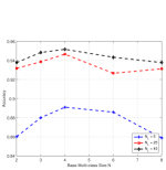
(a) Pendigits.

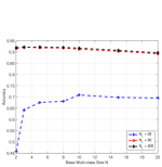
(b) Letters.

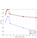
(c) Sector.

(d) Aloi.

Figure 4: Accuracy vs. $N$.

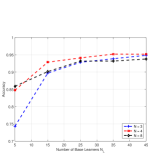
(a) Pendigits.

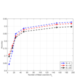
(b) Letters.

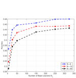
(c) Sector.

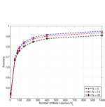
(d) Aloi.

Figure 5: Accuracy vs. $N_{L}$.

VI-B Comparison to State-of-the-art ECOC Strategies.

We compare our proposed $N$-ary ECOC scheme to other state-of-the-art ECOC schemes with different base classifiers including decision tree (DT) [5] and support vector machine (SVM) [6]. The two binary classifiers can be easily extended to a multi-class setting. In particular, we use the multi-class SVM (M-SVM) [8] implemented with the MSVMpack [19]. In addition to the multi-class extension of the two classifiers, we also compare $N$-ary ECOC to OVO, OVA, random ECOC, ECOCONE and DECOC with the two binary classifiers. For random ECOC and $N$-ary ECOC, we report the best results with $N_{L}\leq N_{C}(N_{C}-1)/2$, which is sufficient for conventional random ECOC to reach optimal performance [1, 12]. But for Aloi dataset with 1000 classes, we only report the results for all the ECOC based methods within $N_{L}=1000$ due to its large class size.

VI-B1 Comparison to state-of-the-art ECOC with SVM Classifiers

The classification accuracy of different ECOC coding schemes as well as proposed $N$-ary ECOC with SVM classifiers are presented in Table VII. We observe that OVO has the best and most stable performance on most datasets of all the encoding schemes except for $N$-ary ECOC. This is because all the information between any two classes is used during classification and the OVO coding strategy has no redundancy among different base classifiers. However, it sacrifices efficiency for better performance. It is very expensive for both training and testing when there are many classes in the datasets such as the Auslan, Sector and Aloi. Especially, for Aloi with 1000 classes, it is often not viable to calculate the entire OVO classifications in the real-world application as it would require 499 500 base learners in the pool of possible combinations for training and testing. The performance of OVA is unstable. For the datasets News20 and Sector, OVA even significantly outperforms OVO. However, the performances of OVA on the datasets Vowel, Letters, and Glass are much worse than other encoding schemes. Note that ECOCONE is initialized with OVA. Its performance largely depends on the performance of the initial coding matrix. When OVA performs poorly, ECOCONE also performs poorly. Another problem-dependent coding approach DECOC sets the fixed length of ECOC codes to $N_{C}-1$. Although ECOCONE and DECOC are problem-dependent coding strategies, their performance is not satisfactory in general. We observe that M-SVM achieves better results than ECOC because it considers relationship among classes. However, the training complexity of M-SVM is very high. In contrast to M-SVM, ECOC can be parallelized due to independencies of base tasks. $N$-ary ECOC combines the advantages of both M-SVM and ECOC to achieve better performance.

TABLE VI: Classification accuracy and standard deviation obtained by SVM classifiers for UCI datasets.

Dataset	OVO	OVA	ECOC	DECOC	ECOCONE	M-SVM	Nary-ECOC
Pendigits	93.71 $\pm$ 2.03	$81.75\pm 1.07$	$87.64\pm 1.08$	$72.21\pm 0.88$	$88.84\pm 1.57$	$89.85\pm 1.65$	$93.22\pm 1.71$
Vowel	48.67 $\pm$ 2.63	$30.30\pm 1.42$	$34.28\pm 1.55$	$32.42\pm 1.49$	$31.67\pm 1.75$	$41.67\pm 1.42$	$39.96\pm 2.07$
News20	$68.36\pm 1.70$	$72.65\pm 2.24$	$70.61\pm 1.67$	$66.84\pm 1.90$	$70.78\pm 1.22$	70.78 $\pm$ 0.85	72.79 $\pm$ 1.08
Letters	$81.85\pm 1.26$	$66.93\pm 1.37$	$77.78\pm 1.26$	$68.58\pm 2.35$	$70.56\pm 1.58$	80.16 $\pm$ 2.06	82.27 $\pm$ 1.09
Auslan	$89.94\pm 2.23$	$41.12\pm 1.28$	$83.15\pm 0.84$	$50.86\pm 2.20$	$46.24\pm 1.60$	$90.06\pm 1.58$	91.57 $\pm$ 0.96
Sector	$85.06\pm 1.54$	$89.06\pm 1.35$	$88.01\pm 1.47$	$88.47\pm 1.05$	$89.89\pm 0.88$	$88.75\pm 1.55$	91.05 $\pm$ 1.32
Aloi	91.49 $\pm$ 1.68	$84.26\pm 2.53$	$85.48\pm 1.17$	$82.47\pm 1.05$	$85.09\pm 0.88$	$86.69\pm 1.02$	92.77 $\pm$ 1.86
Glass	61.84 $\pm$ 2.24	$55.00\pm 2.23$	$56.00\pm 0.89$	$52.21\pm 1.21$	$56.84\pm 1.12$	$58.84\pm 2.42$	$56.84\pm 1.56$
Satimage	$85.69\pm 2.57$	$83.11\pm 1.86$	$81.19\pm 1.62$	$82.71\pm 1.44$	$82.56\pm 1.61$	$83.28\pm 0.36$	86.50 $\pm$ 0.93
Usps	$94.30\pm 1.14$	$92.37\pm 1.65$	$90.76\pm 1.45$	$83.11\pm 1.72$	$78.28\pm 1.67$	$92.16\pm 1.27$	96.15 $\pm$ 2.47
Segment	$92.30\pm 1.46$	$92.00\pm 1.89$	$87.80\pm 1.61$	$90.78\pm 1.78$	$78.28\pm 1.23$	$89.96\pm 1.49$	93.60 $\pm$ 1.53
Mean Rank	2.8	4.9	5.1	5.6	5.0	3.0	1.6

TABLE VII: Classification accuracy and standard deviation obtained by CART classifiers for UCI datasets.

Dataset	OVO	OVA	ECOC	DECOC	ECOCONE	M-CART	Nary-ECOC
Pendigits	$93.84\pm 2.33$	$78.12\pm 1.24$	$83.54\pm 1.30$	$81.45\pm 1.38$	$80.53\pm 1.12$	$87.64\pm 1.12$	95.84 $\pm$ 1.08
Vowel	$44.45\pm 1.74$	$33.57\pm 2.31$	$43.65\pm 2.35$	$35.73\pm 1.16$	$36.15\pm 2.25$	$45.45\pm 2.25$	48.50 $\pm$ 1.20
News20	$50.60\pm 1.17$	$45.23\pm 1.15$	$51.29\pm 1.26$	$44.25\pm 2.29$	$50.28\pm 1.37$	$50.83\pm 1.37$	53.71 $\pm$ 1.70
Letters	$81.56\pm 1.30$	$74.69\pm 1.50$	$89.75\pm 1.55$	$78.56\pm 1.05$	$77.10\pm 1.26$	$77.35\pm 1.26$	92.15 $\pm$ 1.92
Auslan	$79.84\pm 2.23$	$72.86\pm 2.04$	$83.15\pm 2.84$	$75.30\pm 1.15$	$75.28\pm 2.36$	$78.89\pm 1.18$	85.17 $\pm$ 1.26
Sector	$39.49\pm 1.33$	$41.89\pm 1.26$	$43.60\pm 1.17$	$44.47\pm 2.35$	$44.29\pm 1.18$	$45.89\pm 2.15$	47.05 $\pm$ 1.27
Aloi	$89.26\pm 1.49$	$72.10\pm 2.60$	$79.41\pm 1.08$	$75.33\pm 2.13$	$72.78\pm 1.80$	$73.00\pm 2.07$	95.13 $\pm$ 1.89
Glass	$52.84\pm 1.15$	$50.12\pm 1.24$	$54.65\pm 1.35$	$52.21\pm 2.38$	$53.02\pm 2.12$	64.00 $\pm$ 2.12	56.00 $\pm$ 1.14
Satimage	$85.70\pm 1.27$	$84.15\pm 1.08$	$85.86\pm 2.75$	$80.37\pm 1.16$	$84.28\pm 2.36$	$83.47\pm 2.36$	86.47 $\pm$ 2.23
Usps	$90.94\pm 2.16$	$80.89\pm 1.47$	$91.95\pm 1.57$	$80.25\pm 1.19$	$80.45\pm 2.36$	$83.54\pm 1.16$	92.77 $\pm$ 1.15
Segment	$93.68\pm 1.25$	$86.45\pm 2.22$	$96.44\pm 2.52$	$80.57\pm 2.16$	$88.78\pm 1.36$	$92.70\pm 1.34$	97.10 $\pm$ 1.28
Mean Rank	3.6	6.3	2.8	5.7	5.1	3.4	1.1

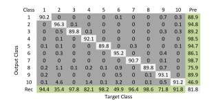
(a) Binary Code.

(b) Ternary Code.

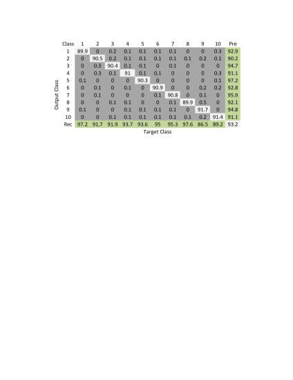
(c) N-ary Code.

Figure 6: Confusion matrix on Pendigits: In confusion matrix, the entry in the ith row and jth column is the percentage of images from class i that are misidentified as class j. Average classification rates for individual classes are listed along the diagonal. The last column and last row are precision (Pre) and recall (Rec) respectively.

VI-B2 Comparison to State-of-the-art ECOC with Decision Tree Classifiers

Next, we compare $N$-ary ECOC with other state-of-the-art coding schemes using binary decision tree classifiers CART [5] as well as its multi-class extension M-CART. We implement it with the CART toolbox with a default setting and the results are reported in Table VII. We observe that binary decision tree classifiers with traditional ECOC strategies are worse than the direct multi-class extension of the decision tree. The decision tree classifiers show better performances than SVM on the Pendigits, Vowel, and Letters datasets. However, it shows very poor performances on high dimensional datasets such as News20 and Sector. This is due to the fact that high-dimensional features often lead to complex tree structure construction. Nevertheless, $N$-ary ECOC still can significantly improve the performance on either traditional coding schemes with binary decision tree learner as well as the multi-class decision tree.

In summary, our proposed $N$-ary ECOC is superior to traditional ECOC encoding schemes and direct multi-class algorithms on most tasks, and provides a flexible strategy to decompose many classes into many smaller multi-class problems, each of which can be independently solved by either M-SVM or M-CART in parallelization.

VI-B3 Discussion on Many class Situation

From the experiments results, we observe that the $N$-ary ECOC shows significant improvement on the Aloi dataset with 1000 classes over other existing coding schemes as well as direct multi-class classification algorithms, especially decision tree classifiers. For the binary or ternary ECOC codes, it is highly possible to assign the same codes to different classes. From the experimental results, we observe the minimum distance $\rho$ for binary and ternary coding are small or even tends to be 0. In other words, the existing coding cannot help the classification algorithms to differentiate some classes. In contrast, $N$-ary with $N_{L}=1000$ and $N=5$, the minimum distance $\rho$ is 741. Thus, it creates codes with larger margins for different classes, whichexplains the superior On the other hand, the direct multi-class algorithms cannot work well when the class size is large. Furthermore, the computation cost for direct multi-class algorithms is in $O(N_{C}^{3})$. When the class size $N_{C}$ is large, the algorithms are expensive to train. On the contrary, random ECOC codes can be easily parallelized due to the independency among the subproblems.

VI-B4 Discussion on Performance on Each Individual Class

To understand the performances of different codes for each individual class, we show the confusion matrix on the Pendigits dataset in Figure 6. First, we observe that binary code (i.e., OVA) has very poor performances on some classes in terms of recall or precision. For example, recall on class 2, 6 and precision on class 10 are below 50%. It can be explained by that as illustrated in Figure 1(b), binary codes may lead to nonseparable cases. Nevertheless, it achieves best classification results on the class 2, 4, 6 and class 9. Compared to the binary code, ternary code (i.e., OVO) largely reduces the bias and improve precision and recall scores on most classes. What is more interesting, when the ternary code and $N$-ary code achieves comparable overall performances, $N$-ary achieves smaller maximal errors. It may be benefited from simpler subtasks created by $N$-ary coding scheme, as shown in Figure 1(d).

VII Conclusions

In this paper, we investigate whether one can relax binary and ternary code design to $N$-ary code design to achieve better classification performance. In particular, we present an $N$-ary coding scheme that decomposes the original multi-class problem into simpler multi-class subproblems. The advantages of such a coding scheme are as follows: (i) the ability to construct more discriminative codes and (ii) the flexibility for the user to select the best $N$ for ECOC-based classification. We derive a base classifier independent generalization error bound for the $N$-ary ECOC classification problem. We show empirically that the optimal $N$ (based on classification performance) lies in $[3,10]$ with some tradeoff in computational cost. Experimental results on benchmark multi-class datasets show that the proposed coding scheme achieves superior prediction performance over the state-of-the-art coding methods. In the future, we will investigate a more efficient realization of $N$-ary coding scheme to improve the prediction speed.

VIII Acknowledgements

This work is done when Dr Joey Tianyi Zhou were at Nanyang Technological University supported by the Research Scholarship. Dr. Ivor W. Tsang is grateful for the support from the ARC Future Fellowship FT130100746 and ARC grant LP150100671. Dr. Shen-Shyang Ho acknowledges the support from MOE Tier 1 Grants RG41/12. Dr. Klaus-Robert M$\ddot{\textrm{u}}$ller gratefully acknowledges partial financial support by DFG, BMBF and BK21 from NRF (Korea).

Joey Tianyi Zhou is a scientist with the Computing Science Department, Institute of High Performance Computing (IHPC), Singapore. Prior to join IHPC, he was a research fellow in Nanyang Technological University (NTU). He received the Ph.D. degree in computer science from NTU, Singapore, in 2015.

Ivor W. Tsang is an Australian Future Fellow and an Associate Professor with the Centre for Quantum Computation and Intelligent Systems, University of Technology at Sydney, Ultimo, NSW, Australia. He received the Ph.D. degree in computer science from the Hong Kong University of Science and Technology, Hong Kong, in 2007. He was the Deputy Director of the Centre for Computational Intelligence, Nanyang Technological University, Singapore. He has authored more than 100 research papers in refereed international journals and conference proceedings, including JMLR, TPAMI, TNN/TNNLS, NIPS, ICML, UAI, AISTATS, SIGKDD, IJCAI, AAAI, ACL, ICCV, CVPR, and ICDM. Dr. Tsang was a recipient of the 2008 Natural Science Award (Class II) from the Ministry of Education, China, in 2009, which recognized his contributions to kernel methods. He was also a recipient of the prestigious Australian Research Council Future Fellowship for his research regarding Machine Learning on Big Data in 2013. In addition, he received the prestigious IEEE TRANSACTIONS ON NEURAL NETWORKS Outstanding 2004 Paper Award in 2006, the 2014 IEEE TRANSACTIONS ON MULTIMEDIA Prized Paper Award, and a number of Best Paper Awards and Honors from reputable international conferences, including the Best Student Paper Award at CVPR 2010, the Best Paper Award at ICTAI 2011, and the Best Poster Award Honorable Mention at ACML 2012. He was also a recipient of the Microsoft Fellowship in 2005 and the ECCV 2012 Outstanding Reviewer Award

Shen-shyang Ho received the BS degree in mathematics and computational science from the National University of Singapore in 1999, and the MS and PhD degrees in computer science from George Mason University in 2003 and 2007, respectively. From August 2007 to May 2010, he was a NASA Postdoctoral Program (NPP) fellow and then a postdoctoral scholar at the California Institute of Technology affiliated to the Jet Propulsion Laboratory (JPL). From June 2010 to December 2012, he was a researcher working on projects funded by NASA at the University of Maryland Institute for Advanced Computer Studies (UMIACS). Currently, he is a tenure-track assistant professor in the School of Computer Engineering at the Nanyang Technological University. His research interests include data mining, machine learning, pattern recognition in spatiotemporal/data streaming settings, and privacy issues in data mining. He is also currently involved in industrial research projects funded by BMW and Rolls-Royces. He has given tutorials at AAAI, IJCNN, and ECML.

Klaus-Robert M$\ddot{\textrm{u}}$ller received the Diploma degree in mathematical physics and the Ph.D. degree in computer science from Technische Universit$\ddot{\textrm{a}}$t Karlsruhe, Karlsruhe, Germany, in 1989 and 1992, respectively. He has been a Professor of computer science with Technische Universit$\ddot{\textrm{a}}$t Berlin, Berlin, Germany, since 2006, and he is directing the Bernstein Focus on Neurotechnology Berlin, Berlin. Since 2012, he has been a Distinguished Professor with Korea University, Seoul, Korea, within the WCU Program. After a Post-Doctoral at GMD-FIRST, Berlin, he was a Research Fellow with the University of Tokyo, Tokyo, Japan, from 1994 to 1995. In 1995, he built up the Intelligent Data Analysis Group, GMD-FIRST (later Fraunhofer FIRST) and directed it until 2008. From 1999 to 2006, he was a Professor with the University of Potsdam, Potsdam, Germany. His current research interests include intelligent data analysis, machine learning, signal processing, and brain computer interfaces. Dr. M ller received the Olympus Prize by the German Pattern Recognition Society, DAGM, in 1999, and the SEL Alcatel Communication Award in 2006. In 2012, he was elected to be a member of the German National Academy of Sciences Leopoldina.

References

- [1] Erin L. Allwein, Robert E. Schapire, and Yoram Singer. Reducing multiclass to binary: a unifying approach for margin classifiers. J. Mach. Learn. Res., 1:113–141, September 2001.
- [2] Mohammad Ali Bagheri, Gholam Ali Montazer, and Ehsanollah Kabir. A subspace approach to error correcting output codes. Pattern Recognition Letters, 34(2):176 – 184, 2013.
- [3] S. Bengio, J. Weston, and D. Grangier. Label embedding trees for large multi-class tasks. In NIPS, pages 163–171, 2010.
- [4] A. Beygelzimer, J. Langford, Y. Lifshits, G. Sorkin, and A. Strehl. Conditional probability tree estimation analysis and algorithms. In UAI, pages 51–58, 2009.
- [5] Leo Breiman, J. H. Friedman, R. A. Olshen, and C. J. Stone. Classification and Regression Trees. Statistics/Probability Series. Wadsworth Publishing Company, Belmont, California, U.S.A., 1984.
- [6] Chih-Chung Chang and Chih-Jen Lin. Libsvm: A library for support vector machines. ACM Trans. Intell. Syst. Technol., 2(3):27:1–27:27, May 2011.
- [7] T. Cover and P. Hart. Nearest neighbor pattern classification. Information Theory, IEEE Transactions on, 13(1):21–27, January 1967.
- [8] Koby Crammer and Yoram Singer. On the algorithmic implementation of multiclass kernel-based vector machines. J. Mach. Learn. Res., 2:265–292, March 2002.
- [9] J. Deng, S. Satheesh, A. Berg, and L. Fei-Fei. Fast and balanced: Efficient label tree learning for large scale object recognition. In NIPS, 2011.
- [10] Thomas G. Dietterich and Ghulum Bakiri. Error-correcting output codes: A general method for improving multiclass inductive learning programs. In AAAI, pages 572–577. AAAI Press, 1991.
- [11] Thomas G. Dietterich and Ghulum Bakiri. Solving multiclass learning problems via error-correcting output codes. J. Artif. Intell. Res., 2:263–286, 1995.
- [12] S. Escalera, O. Pujol, and P. Radeva. On the decoding process in ternary error-correcting output codes. Pattern Analysis and Machine Intelligence, IEEE Transactions on, 32(1):120–134, 2010.
- [13] Sergio Escalera and Oriol Pujol. Ecoc-one: A novel coding and decoding strategy. In ICPR, pages 578–581, 2006.
- [14] Sergio Escalera, Oriol Pujol, and Petia Radeva. Error-correcting ouput codes library. J. Mach. Learn. Res., 11:661–664, March 2010.
- [15] T. Gao and D. Koller. Discriminative learning of relaxed hierarchy for large-scale visual recognition. In ICCV, pages 2072–2079, 2011.
- [16] Nicolás García-Pedrajas and Domingo Ortiz-Boyer. An empirical study of binary classifier fusion methods for multiclass classification. Inf. Fusion, 12(2):111–130, April 2011.
- [17] Robert Jenssen, Marius Kloft, Alexander Zien, Soeren Sonnenburg, and Klaus-Robert Müller. A scatter-based prototype framework and multi-class extension of support vector machines. PloS one, 7(10):e42947, 2012.
- [18] Josef Kittler, Reza Ghaderi, Terry Windeatt, and Jiri Matas. Face verification via error correcting output codes. Image Vision Comput., 21(13-14):1163–1169, 2003.
- [19] F. Lauer and Y. Guermeur. MSVMpack: a multi-class support vector machine package. Journal of Machine Learning Research, 12:2269–2272, 2011.
- [20] Xu-Ying Liu, Qian-Qian Li, and Zhi-Hua Zhou. Learning imbalanced multi-class data with optimal dichotomy weights. In Data Mining (ICDM), 2013 IEEE 13th International Conference on, pages 478–487. IEEE, 2013.
- [21] Gholam Ali Montazer, Sergio Escalera, et al. Error correcting output codes for multiclass classification: Application to two image vision problems. In AISP, pages 508–513. IEEE, 2012.
- [22] Oriol Pujol, Petia Radeva, and Jordi Vitrià. Discriminant ECOC: a heuristic method for application dependent design of error correcting output codes. In IEEE Transaction on Pattern Analysis and Machine Intelligence, pages 1007–1012, 2006.
- [23] J. R. Quinlan. Induction of decision trees. Mach. Learn., 1(1):81–106, March 1986.
- [24] Anderson Rocha and Siome Goldenstein. Multiclass from binary: Expanding one-vs-all, one-vs-one and ecoc-based approaches. IEEE Transactions on Neural Networks and Learning Systems, 25(2):289–302, 2014.
- [25] Jiang Su and Harry Zhang. A fast decision tree learning algorithm. In Proceedings of the 21st National Conference on Artificial Intelligence - Volume 1, AAAI’06, pages 500–505. AAAI Press, 2006.
- [26] Ivor W. Tsang, James T. Kwok, and Pak-Ming Cheung. Core vector machines: Fast SVM training on very large data sets. Journal of Machine Learning Research, 6:363–392, 2005.
- [27] Elif Derya Übeyli. Ecg beats classification using multiclass support vector machines with error correcting output codes. Digital Signal Processing, 17(3):675–684, 2007.
- [28] Xiaoyu Wang, Tianbao Yang, Guobin Chen, and Yuanqing Lin. Object-centric sampling for fine-grained image classification. arXiv preprint arXiv:1412.3161, 2014.
- [29] Jian-Bo Yang and Ivor W. Tsang. Hierarchical maximum margin learning for multi-class classification. In UAI, 2011.
- [30] Bangpeng Yao, Aditya Khosla, and Li Fei-Fei. Combining randomization and discrimination for fine-grained image categorization. In Computer Vision and Pattern Recognition (CVPR), 2011 IEEE Conference on, pages 1577–1584. IEEE, 2011.
- [31] Zhou Yu, Deng Cai, and Xiaofei He. Error-correcting output hashing in fast similarity search. In Proceedings of the Second International Conference on Internet Multimedia Computing and Service, ICIMCS ’10, pages 7–10, New York, NY, USA, 2010. ACM.
- [32] Bin Zhao and Eric P. Xing. Sparse output coding for large-scale visual recognition. In CVPR, pages 3350–3357. IEEE, 2013.
- [33] Guoqiang Zhong and Mohamed Cheriet. Adaptive error-correcting output codes. In IJCAI, pages 1932–1938, 2013.
- [34] Guoqiang Zhong and Cheng-Lin Liu. Error-correcting output codes based ensemble feature extraction. Pattern Recognition, 46(4):1091–1100, 2013.