Michelson–Morley experiment, Doppler effect, aberration of light and the aether concept

Abstract

After an overview of various citations relevant in the context of photon propagation, the relativistic Doppler effect and the addition theorem of velocities are first derived taking into account momentum and energy conservation. Clocks and the aberration of light are treated next, before the lengths of rods and the Lorentz transformations are discussed. The Michelson–Morley experiment is described at rest and in motion with respect to a preferred aether system, first under the assumption of an operation in vacuum. It is concluded that the aether concept is fully consistent with the formal application of the Special Theory of Relativity (STR). Whether a determination of the speed of the laboratory system relative to the aether is possible, is considered next either for an operation of the experiment in vacuum or in a medium with an index of refraction not equal to one. In both cases, the answer appears to be negative.

Last updated on

Keywords radiation: dynamics – relativistic
processes – techniques: interferometric – cosmology: theory

1 Introduction

The following statement (Einstein, 1917, p. 126) highlights the importance with regard to the Doppler effect – discovered by Doppler (1842) – and the aberration – first described by Bradley (1727):

1. Whatever will eventually be the theory of electromagnetic processes, the D o p p l e r principle and the aberration law will continue to be valid, […].

Since Michelson & Morley (1887) carried out their famous experiment, the discussion remains inconclusive on whether or not the vacuum is filled with some kind of aether. A recent publication recounts this history (Kragh and Overduin, 2014).

First we want to refer to early statements by Einstein and others concerning the aether in the framework of the Special Theory of Relativity (STR) (Einstein, 1908, p. 413):

1. Only the concept of a light aether as carrier of the electric and magnetic forces is not consistent with the theory discussed here; […].

von Laue (1908) discussed the Lorentz contraction in the context of the electron theory (cf. Abraham, 1903) and the STR:

1. Both theories […] agree. The only difference concerns the shapes of moving charges; one theory assumes that they are not affected, whereas the other gives a contraction in the direction of motion. […].

In this paper, we will assume that the shapes are not affected. The alternative is the standard treatment based on the Lorentz contraction. it would lead to slightly modified equations, but would not affect the main results.

In response to critical remarks by Wiechert (1911), von Laue (1912) concluded that the existence of the aether is not a physical, but a philosophical problem. However, von Laue (1959, p. 83) later differentiated between the physical world and the mathematical formulation of STR:

1. It owes its elegant mathematical guise Hermann MINKOWSKI who […] introduced time as fourth coordinate on the same footing with the three spatial coordinates to form a four-dimensional “World”. However, this is only a valuable mathematical trick; deeper insight, which some people want to see behind it, is not involved.

Schröder (1990) discussed Wiechert’s support of the aether concept by presenting unpublished material from about 1919 to 1922 containing the following two statements:

1. Einstein’s theory of relativity caused a sudden setback at the end of 1905 (cf. Einstein, 1905b). Admittedly Lorentz’ Theory was formally very much improved, and based on the options of the Lorentz transformations, Einstein and others have erected both a beautiful and extended building that is without doubt of great and lasting value for physics. However, in addition, an epistemological foundation was added with new relativistic ideas leading to inconsistencies with aether concepts.

2. On the nature of the substratum of the world two ideas are in conflict: the concept of spacetime und the aether.

In contrast to earlier statements, Einstein said at the end of his speech in Leiden (Einstein, 1920):

1. According to the General Theory of Relativity (GTR) a space without aether cannot be conceived; […].

For further quotations of the speech see Granek (2001) and Kostro (2004) for other statements by Einstein on the aether concept.

In 1927 Michelson confessed at a meeting in Pasadena in the presence of H.A. Lorentz:

1. ‘Talking in terms of the beloved old aether (which is now abandoned, though I personally still cling a little to it), […]’ (Michelson et al., 1928, p. 342).

Dirac (1951, p. 906) wrote in a letter to Nature:

1. ‘If one examines the question in the light of present-day knowledge, one finds that the æther is no longer ruled out by relativity, and good reasons can now be advanced for postulating an æther.’

and Builder (1958) stated in the summary:

1. ‘There is therefore no alternative to the ether hypothesis.’

Considering these statements, it is only appropriate to revisit the relationship of the mathematical formulation of the STR and its physical contents as well as to reconsider the aether concept in this paper. We will denote our laboratory system with S. It contains physical devices, such as rods, clocks, photon emitters and detectors. As far as photons are concerned, we will frequently refer to the wave-particle dualism (Einstein, 1905a) by quoting their energy $E_{\nu}=h\,\nu$, where $h=6.626\,070\,040\times 10^{-34}$ J s is Planck’s constant (CODATA, 2014) and, at the same time, characterize them by their frequency $\nu$ and wavelength $\lambda$. The System S is either at rest in a putative aether system S_p or moves with a velocity $v$ relative to S_p.

The important questions are whether such a preferred aether system, in which the propagation of photons is isotropic with a speed of light in vacuum $c_{0}~{}=~{}299\,792\,458~{}{\ \mathrm{m}}\,{\ \mathrm{s}}^{-1}$ (exact) (BIPM, 2006, p. 22) is compatible with physical experiments in laboratory systems and if – should the answer be in the affirmative – experimental methods can be devised to determine the speed $v$.

Before we embark on this exercise, an interesting remark by Fermi (1932, pp.105/106) should be recalled:

1. ‘The change of frequency of the light emitted from a moving source is very simply explained by the wave theory of light. But it finds also a simple, though apparently very different, explanation in the light-quantum theory; it can be shown that the Doppler effect may be deduced from the conservation of energy and momentum in the emission process.
   Let us consider an atom A with two energy levels $w_{1}$ and $w_{2}$; the frequency emitted by the atom when it is at rest is then

   $$\quad\quad\quad\quad\quad\quad\quad\quad\quad\nu=(w_{2}-w_{1})/h.$$

   Let us now suppose that the atom is excited and that it moves with velocity $V$; its total energy is then:

   $$\quad\quad\quad\quad\quad\quad\quad\quad\quad w_{2}+\frac{1}{2}\,m\,V^{2}.$$

   At a given instant the atom emits, on jumping down to the lower state, a quantum of frequency $\nu^{\prime}$; the recoil of the emitted quantum produces a slight change of the velocity, which after the emission becomes $V^{\prime}$; the energy of the atom is then $w_{1}+\frac{1}{2}\,m\,V^{\prime 2}$. We get therefore from conservation of energy

   $$h\,\nu^{\prime}=(w_{2}+\frac{1}{2}\,m\,V^{2})-(w_{1}+\frac{1}{2}\,m\,V^{\prime 2})=\quad\quad\quad$$

   $$\quad\quad\quad\quad\quad\quad\quad\quad h\,\nu+\frac{1}{2}\,m\,(V^{2}-V^{\prime 2}).$$

   The conservation of momentum gives:

   $$\quad\quad\quad\quad\quad\quad\quad\quad\quad m\,\mbox{\boldmath$V^{\prime}$}=m\,\mbox{\boldmath$V$}-\frac{h\,\mbox{\boldmath$\nu^{\prime}$}}{c}$$

   where the bold face letters mean vectors. Taking the square we get:

   $$\quad\quad\quad\quad m^{2}V^{\prime 2}=m^{2}V^{2}+\frac{h^{2}\nu^{\prime 2}}{c^{2}}-2\,m\,V\,\frac{h\,\nu}{c}\,\cos\theta$$

   $\theta$ being the angle between the velocity and the direction of emission. From this equation and (76) we get, neglecting terms in $1/c^{2}$:

   $$\quad\quad\quad\quad\quad\quad\quad\nu^{\prime}=\nu\,\left(1+\frac{V}{c}\,\cos\theta\right)$$

   which is the classic formula for the Doppler effect to a nonrelativistic approximation.’

2 Relativistic Doppler effect and addition theorem of velocities

Guided by Fermi’s explanation of the Doppler effect, we will now derive a relativistic formulation under the assumption of the preferred system S_p.

An atom A with mass $m$ in its ground state at rest in S_p has an energy of

$$E_{0}=m\,c^{2}_{0}~{}.$$ (1)

The energy-momentum relation for a particle in motion is (cf. Einstein, 1905a, c; Dirac, 1936; Okun, 1989):

$$E^{2}=m^{2}\,c^{4}_{0}+\mbox{\boldmath$p$}^{2}c^{2}_{0}=m^{2}\,c^{4}_{0}+p^{2}c^{2}_{0}~{}.$$ (2)

For the atom A with a speed $v$ relative to System S_p, the energy $E$ in S_p can be found with the help of the momentum vector

$$\mbox{\boldmath$p$}=\mbox{\boldmath$v$}\,\frac{E}{c^{2}_{0}}\quad\quad\quad\left(~{}|\mbox{\boldmath$p$}|=p=\beta\,\frac{E}{c_{0}}~{}\right)$$ (3)

with $\beta=v/c_{0}$ and $|\beta|<1$. Combining Eqs. (2) and (3) leads to

$$E=\frac{m\,c^{2}_{0}}{\sqrt{1-\beta^{2}}}=\gamma\,m\,c^{2}_{0}~{},$$ (4)

where

$$\gamma=\frac{1}{\sqrt{1-\beta^{2}}}$$ (5)

is the Lorentz factor with $1\leq\gamma<\infty$ and

$$E-E_{0}=m\,c^{2}_{0}\,(\gamma-1)=E_{\rm kin}$$ (6)

is the kinetic energy.

If the atom is in an excited state with an excitation energy $\mathnormal{\Delta}E=E_{\nu}=h\,\nu$, if measured in the rest frame of the atom, Eq. (2) reads

$$(E^{*})^{2}=(m^{*})^{2}c^{4}_{0}+(p^{*})^{2}c^{2}_{0}~{},$$ (7)

with a mass (cf. Einstein, 1905c, p. 641)(von Laue, 1920, p. 394)

$$m^{*}=m+\frac{\mathnormal{\Delta}E}{c^{2}_{0}}$$ (8)

and a momentum

$$p^{*}=\beta\,\frac{E^{*}}{c_{0}}~{},$$ (9)

cf. Eq. (3). According to Eq. (4), the energy can also be expressed with the Lorentz factor $\gamma$ as:

$$E^{*}=\gamma\,m^{*}c^{2}_{0}=\gamma\,(m\,c^{2}_{0}+\mathnormal{\Delta}E)~{}.$$ (10)

During de-excitation of the atom, a photon will be emitted. For the sake of simplicity, only directions parallel or anti-parallel to an $x$ axis will be considered. Nevertheless two effects have to be evaluated: the motion of System S, in which atom A is at rest, relative to the preferred System S_p and the recoil on the emitting atom.

Conservation of momentum and  energy in S_p requires

$$p^{\pm}=p^{*}\mp\frac{h\,\nu^{\pm}}{c_{0}}$$ (11)

and

$$E^{\pm}=E^{*}-h\,\nu^{\pm}~{}.$$ (12)

The notations $p^{+}$, $h\,\nu^{+}$ indicate the momentum and energy, respectively, of a photon propagating in the positive $x$ direction and $p^{-}$ and $h\,\nu^{-}$ the reverse.

The recoil can conveniently be calculated by first assuming $v=0$, i.e., the system S coincides with S_p and the photon emission is isotropic in both systems. With this assumption, Eqs. (11) and (12) reduce to

$$p^{\pm}_{0}=\mp\frac{h\,\nu^{\pm}_{0}}{c_{0}}$$ (13)

and

$$E^{\pm}_{0}=m\,c^{2}_{0}+\mathnormal{\Delta}E-h\,\nu^{\pm}_{0}~{}.$$ (14)

Applying Eq. (2) to this case gives:

$$(E^{\pm}_{0})^{2}=m^{2}\,c^{4}_{0}+(p^{\pm}_{0})^{2}c^{2}_{0}~{}.$$ (15)

Eliminating $p^{\pm}_{0}$ and $E^{\pm}_{0}$ with the help of Eqs. (13) and (14), we get the the recoil redshift after a short calculation and the (trivial) result that it does not depend on the direction of the emission in this case:

$$\nu^{\pm}_{0}=\nu\,\frac{m\,c^{2}_{0}+\mathnormal{\Delta}E/2}{m\,c^{2}_{0}+\mathnormal{\Delta}E}\approx\nu\,\left(1-\frac{1}{2}\,\frac{\mathnormal{\Delta}E}{m\,c^{2}_{0}}\right)~{},$$ (16)

where the approximation is valid for small $\mathnormal{\Delta}E/(m\,c^{2}_{0})$.

In the general case with a speed $v\neq 0$ of S with respect to the preferred System S_p, the photon energy $h\,\nu^{\pm}$ and the momentum $h\,\nu^{\pm}/c_{0}$ must now be evaluated in S_p, in which the propagation is assumed to occur.

Taking the square of Eq. (12) gives – together with Eq. (2) and the consideration that after the emission the mass of the atom is again $m$ – the relation:

$$m^{2}\,c^{4}_{0}+(p^{\pm})^{2}c^{2}_{0}=$$

$$(E^{*})^{2}-2\,E^{*}h\,\nu^{\pm}+(h\,\nu^{\pm})^{2}~{}.$$ (17)

The elimination of the momentum and energy terms using Eqs. (8) to (11) leads after a lengthy calculation to

$$\mathnormal{\Delta}E~{}(m\,c^{2}_{0}+\frac{\mathnormal{\Delta}E}{2})=h\,\nu^{\pm}\,\gamma\,(m\,c^{2}_{0}+\mathnormal{\Delta}E)\,(1\mp\beta)~{},$$ (18)

and finally, with $\mathnormal{\Delta}E=h\,\nu$ in the rest system of the emitter, to the result that the relativistic Doppler shift depends on the direction and the emission becomes anisotropic:

$$\nu^{\pm}=\nu\,\frac{m\,c^{2}_{0}+\mathnormal{\Delta}E}{m\,c^{2}_{0}+\mathnormal{\Delta}E}\,\frac{\sqrt{1-\beta^{2}}}{1\mp\beta}=\nu^{\pm}_{0}\,\displaystyle{\sqrt{\frac{1\pm\beta}{1\mp\beta}}}~{},$$ (19)

where the definition of $\nu^{\pm}_{0}$ agrees with that in Eq. (16). In what follows, we will generally neglect any recoil, for instance, by employing the Mößbauer effect (Mössbauer, 1958) to obtain a very large effective mass in Eqs. (16) and (19). Eq. (19) then is equivalent to the relativistic Doppler equation which Einstein (1905b, p. 902) derived for the separation of a detector with constant speed $v=\beta\,c_{0}$ relative to an emitter:

$$\nu^{-}=\nu\,\sqrt{\frac{1-\beta}{1+\beta}}~{}.$$ (20)

The Doppler effect followed in Einstein’s treatment from the application of the Lorentz transformations (cf. Poincaré, 1905, p. 1505) to Lorentz’ electrodynamics (Lorentz, 1895, 1904), whereas Eq. (19) is a consequence of the momentum and energy conservation.

The formulation of the detection of the photons with frequencies $\nu^{\pm}$ would have required a similar treatment, but is simplified by assuming no recoil and $\nu=\nu^{\pm}_{0}$. If the detector is – together with the emitter – at rest in S and, therefore, also moving in S_p with $v$, the reverse of Eq. (19) shows that the energy $h\,\nu$ will be absorbed:

$$\nu^{\pm}\,\displaystyle{\sqrt{\frac{1\mp\beta}{1\pm\beta}}}=\nu\,\displaystyle{\sqrt{\frac{1\pm\beta}{1\mp\beta}}}\displaystyle{\sqrt{\frac{1\mp\beta}{1\pm\beta}}}=\nu~{}.$$ (21)

It is noteworthy that an iterative application of Eq. (19) (again with the simplification $\nu^{\pm}_{0}=\nu$) will yield the velocity addition theorem for parallel velocities. For later applications, we write it in the form:

$$w_{y}=\frac{u_{x}+v}{1+\displaystyle{\frac{u_{x}\,v}{c^{2}_{0}}}}~{}~{}~{}~{}~{}~{}{\rm or}~{}~{}~{}~{}~{}~{}\beta_{y}=\frac{\beta_{x}+\beta}{1+\beta_{x}\,\beta}~{},$$ (22)

where $\beta_{x}=u_{x}/c_{0}$ and $\beta_{y}=w_{y}/c_{0}$ with indices $x$ and $y$ as required for a unique formulation.

To prove the above statement, e.g., for positive velocities, we apply the Doppler Eq. (19) first with $\beta_{0}=u_{0}/c_{0}$ and then with $\beta=v/c_{0}$, cf. Eq. (3):

$$\nu^{+}=\nu\,\displaystyle{\sqrt{\frac{1+\beta_{0}}{1-\beta_{0}}}\,\sqrt{\frac{1+\beta}{1-\beta}}}=\nu\,\sqrt{\displaystyle{\frac{1+\displaystyle{\frac{\beta_{0}+\beta}{1+\beta_{0}\,\beta}}}{1-\displaystyle{\frac{\beta_{0}+\beta}{1+\beta_{0}\,\beta}}}}}~{}.$$ (23)

Consequently, we obtain $\nu^{+}$ from

$$\nu^{+}=\nu\,\displaystyle{\sqrt{\frac{1+\beta_{3}}{1-\beta_{3}}}}~{},$$ (24)

where $\beta_{3}$ is

$$\beta_{3}=\frac{w_{3}}{c_{0}}=\frac{\beta_{0}+\beta}{1+\beta_{0}\,\beta}$$ (25)

consistent with Eq. (22). The theorem thus also follows from energy and momentum conservation during the photon emission. The derivation of Eq. (23) assumed that $|\beta_{0}|<1$ and $|\beta|<1$. If either $|\beta_{0}|$ or $|\beta|$ is approaching the limit 1, $|\beta_{3}|$ also goes to 1.

3 Clocks and aberration

In the previous section, we have postulated that the preferred System S_p exists with an isotropic speed of light in vacuum of $c_{0}=\nu\,\lambda$, where $\nu$ and $\lambda$ are the frequency and wavelength of an electromagnetic wave.

This assumption is consistent with the more general synchronization scheme of many clocks at rest in an inertial system by Einstein (1908, p. 415) in order to define a time required by physical applications:

1. Let two points $A$ and $B$ with a separation $r$, at rest in a coordinate system, be equipped with clocks. If the clock at $A$ indicates $t_{A}$, when a light beam propagating through the vacuum in the direction $A\,B$ reaches point $A$, and if $t_{B}$ is the reading of clock $B$, when the beam arrives at $B$, then it should always be $r/(t_{B}-t_{A})=c$, whatever might be the movements of the emitting source or other bodies.

What is a clock? The next two statements suggest that Einstein (1907) considered in most cases atomic oscillators as clocks:

1. Mr. J. Stark (1907) demonstrated in a paper, which appeared last year, that the moving positive ions of canal rays emit line spectra by confirming and measuring the Doppler effect. He also performed investigations with a view to find and study a second-order effect (proportional to $(v/V)^{2}$). Since the experimental setup was not designed for this special purpose, a definite result was not obtained.

2. In Einstein (1908, p. 422) we find:
   Since the oscillation process corresponding to a spectral line has probably to be considered as an intra-atomic process, the frequency of which is determined solely by the ion, we can regard such an ion as a clock with a certain frequency $\nu_{0}$.

However, it is obvious that a clock, in addition, needs a counter to number the periods.

1. ‘A clock therefore produces a time scale (its proper time, in relativistic terminology)’ (Audoin & Guinot, 2001).

Ives and Stilwell (1941, p. 374) were successful in measuring the second-order effect mentioned by Einstein (1907), but summarized the observations by the ambiguous statement:

1. ‘The net result of this whole series of experiments is to establish conclusively that the frequency of light emitted by moving canal rays is altered by the factor $(1-v^{2}/c^{2})^{1/2}$.’

On page 369 the authors refer to their earlier paper (Ives and Stilwell, 1938), where unfortunately conflicting equations $\lambda=\lambda_{0}\,(1-V^{2}/c^{2})^{1/2}$ on page 216 and $\nu=\nu_{0}\,(1-V^{2}/c^{2})^{1/2}$ on page 226 are given. The confusion is augmented by the explanation of the second equation:

1. ‘The present experiment establishes this rate as according to the relation $\nu=\nu_{0}\,(1-V^{2}/c^{2})^{1/2}$ , where $\nu_{0}$ the frequency of the clock when stationary in the ether, $\nu$ its frequency in motion.’

In line with the results of Sect. 2, the last phrase should be modified: In an inertial system in which the atom is moving with $v$ an energy of

$$h\,\nu=h\,\nu_{0}/\gamma$$ (26)

will be emitted by the atom. The balance is taken up by the kinetic energy of the atom.

Saathoff et al. (2011) confirmed the prediction of STR on a level of $<8\times 10^{-8}$ by measuring the Doppler shifts of moving Li⁺ ions in an Ives–Stilwell-type experiment in line with the relativistic Doppler formulae:

$${\rm(a)}~{}~{}\nu_{0}=\nu_{\rm r}^{-}\,\gamma\,(1+\beta)~{}~{}{\rm and}~{}~{}{\rm(b)}~{}~{}\nu_{0}=\nu_{\rm r}^{+}\,\gamma\,(1-\beta)~{},$$ (27)

where $\nu_{0}$ is the frequency in the frame S of the ion and $\nu_{\rm r}^{-}$ and $\nu_{\rm r}^{-}$ the frequencies in a frame S_p. Adding the Eqs. (27a) and (b) shows that the mean value of the energies $h\,\nu_{\rm r}^{-}$ and $h\,\nu_{\rm r}^{+}$ is consistent with Eq. (26).

The general aberration relation is

$$\cos\vartheta=\frac{\cos\vartheta^{+}-\beta}{1-\beta\cos\vartheta^{+}}~{},$$ (28)

where $\vartheta^{+}$ is the angle of light propagation in an inertial System S_p with respect to the direction of the motion of an inertial system S, and $\vartheta$ the corresponding angle in the moving system. It was also obtained by Einstein (1908, p. 425) from the Lorentz transformations. Resolving Eq. (28) for $\cos\vartheta^{+}$ gives the reverse aberration formula:

$$\cos\vartheta^{+}=\frac{\cos\vartheta+\beta}{1+\beta\cos\vartheta}~{}.$$ (29)

For the special case of $\vartheta=90\hbox{${}^{\rm o}$}$, i.e. $\cos\vartheta=0$ it is $\cos\vartheta^{+}=\beta$. It can easily be demonstrated that this follows from energy and momentum conservation as well.

Let an excited atom with a large mass $m$ (so that its recoil can be neglected) and an excitation energy $h\,\nu$ move with a velocity $v$ in S_p. Assume a photon emission perpendicular to $v$ as seen from the moving atom. Its energy is given by Eq. (10) and its momentum by Eq. (9). The emitted photon has an energy of $\Delta E=E^{*}-\gamma\,m\,c^{2}_{2}=\gamma\,h\,\nu$ and, consequently, the magnitude of its momentum vector is $\gamma\,h\,\nu/c_{0}$. The momentum of the atom changes parallel to the velocity by $\beta\,\gamma\,m\,c_{0}-p^{*}=-\beta\,\gamma\,h\,\nu/c_{0}$. Momentum conservation thus requires a momentum component of the photon parallel to $v$ of $\beta\,\gamma\,h\,\nu/c_{0}$. This yields together with its magnitude $\cos\vartheta^{+}=(\beta\,\gamma\,h\,\nu/c_{0})/(\gamma\,h\,\nu/c_{0})=\beta$.

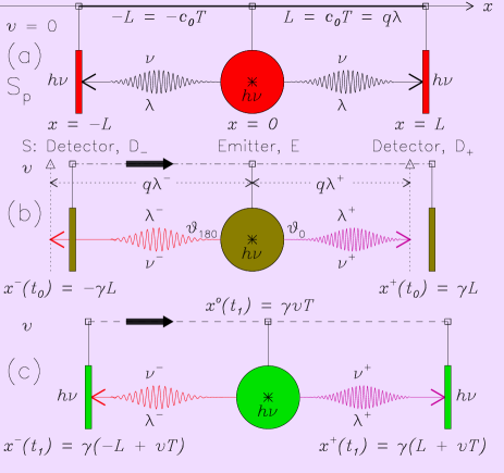
Fig. 1 : In Panel (a), an emitter (circle) is located at $x_{0}=0$ and radiates photons at time $t_{0}=0$ in $+$ or $-$ direction. They are detected by the detectors D_- and D₊ (rectangles) at $x=\pm L$, respectively, after travelling a time $T$ in the preferred system S_p – indicated by the violet shading. The number of wavelengths in $L$ is denoted by $q$. In Panels (b) and (c), the arrangement of emitter and detectors (System S) is shown in S_p, when moving with a velocity $v$ along the $x$-axis. Panel (b) illiustrates the situation at the emission of the photons; together with their potential subsequent propagation in S_p with $q$ wavelengths $\lambda^{\pm}$ within $T^{\pm}=T\,\sqrt{(1\mp\beta)/(1\pm\beta)}$. Panel (c) depicts the system at the time $t_{1}$ of the detection of the photons, when the emitter is located at $x^{\rm o}$.

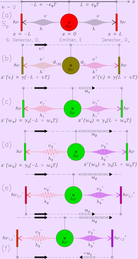
Fig. 2 : As in Fig. 1, a rod of length $2\,L$ is equipped with a source emitting photons with energy $h\,\nu$ in the corresponding rest frame of the emitter and two detectors at the ends. In Panel (a), the rod is at rest in the preferred System S_p – indicated again by the violet shading. In Panel (b), as in Fig. 1(c), the emitter-detector frame S is now moving with an unknown speed $v$ (solid arrow) relative to S_p in the positive $x$ direction. Detection of the photons will then occur at $x^{\pm}(v)$ after times $T^{\pm}(v)$ as seen from S_p, in which the photon propagation is assumed to happen. In Panels (c) to (f), the emitter and the detectors are, in addition, moving relative to S with speeds of $\pm u_{1}$ and $u_{2}$, respectively, which can directly be observed. Their speeds $w^{\pm}_{1}$ and $w_{2}$ relative to S_p can then be calculated with the help of the addition theorem, cf. Eq. (25). The detected energies are calculated in the text.

4 Rods and the Lorentz transformations

Eddington (1923, p. 392) felt that:

1. ‘Size is determined by reference to material standards, and we must not imagine that there can be any definition of size which dispenses with this reference to material objects.’

Nevertheless two alternative methods have been used since: (1) The wavelength of crypton 86 from 1960 to 1983 and (2) the present method based on clocks and the speed of light in vacuum (SI; BIPM, 2006). Eddington had, however, qualified his conclusion by adding:

1. ‘No alternative method can be accepted unless it has been proved to be equivalent to this.’

Lorentz said at the Pasadena conference in 1927 about the contraction hypothesis as an explanation of the Michelson–Morley experiment (Michelson et al., 1928, p. 551):

1. ‘We are thus led to the ordinary theory of the experiment, which would make us expect a displacement of the fringes, the absence of which is accounted for by the well-known contraction hypothesis (Lorentz contraction).
   Asked if I consider this contraction as a real one, I should answer “yes.” It is as real as anything that we can observe.’

A few years before this conference, von Laue (1921, p. 92) remarked on the Lorentz contraction:

1. If we set the body in motion without changing its shape, i.e. with the old positions of the atoms, then is it possible that the forces could vary in the same way as the forces between charges. […] If they are of electromagnetic nature, a rule derived by H.A. Lorentz says that the Lorentz contraction results.

A rod of length $2\,L$ aligned parallel to the $x$-axis of an inertial system S with an emitter of photons with an energy $h\,\nu$ in S at the centre and detectors at both ends is first assumed to be at rest in S_p in Fig. 1(a). For photons propagating in both directions along the rod, we can write with a certain number $q$

$$\pm L=\pm c_{0}\,T=\pm q\,\lambda=\pm q\,\frac{c_{0}}{\nu}~{},$$ (30)

where $T$ is the travel time equal in both directions with $\pm c_{0}$ in the preferred system. If this arrangement is now moving along the $x$-axis with an (unknown) velocity $v$ relative to S_p, the number $q$ of wavelengths can, at least in principle, be counted and, therefore, cannot depend on the state of motion. For this configuration, the longitudinal Doppler effect must be considered, cf. Eq. (19). As shown in Sect. 2, the frequency shifts for the forward and backward directions follow directly from the conservation of energy and momentum of the emitted photons. We first discuss the forward direction:

$$\nu^{+}=\nu\,\gamma\,(1+\beta)=\nu\,\displaystyle{\sqrt{\frac{1+\beta}{1-\beta}}}$$ (31)

with $c_{0}=\nu^{+}\,\lambda^{+}$ in the preferred System S_p, we get

$$\lambda^{+}=\frac{c_{0}}{\nu}\displaystyle{\sqrt{\frac{1-\beta}{1+\beta}}}$$ (32)

and, with an invariant number $q$, a distance along this section of the rod of

$$L^{+}=q\,\lambda^{+}=q\,\frac{c_{0}}{\nu}\,\displaystyle{\sqrt{\frac{1-\beta}{1+\beta}}}=L\,\displaystyle{\sqrt{\frac{1-\beta}{1+\beta}}}$$ (33)

in the time $T^{+}$, cf. Fig. 1(b). Note that the photon travels after the emission in the preferred System S_p with speed $c_{0}$, while the rod in the laboratory system S moves forward with $v$. The question when and where the photon reaches the front end of the moving rod can be answered with the help of the paradox “Achilles and the Tortoise” formulated by Zeno of Elea. With $\beta=v/c_{0}$ it will be at

$$T_{\rm S}=T^{+}\,(1+\beta+\beta^{2}+\beta^{3}+...)=\frac{T^{+}}{1-\beta}=\gamma\,T~{}$$ (34)

and

$$L_{\rm S}=L^{+}\,(1+\beta+\beta^{2}+\beta^{3}+...)=\frac{L^{+}}{1-\beta}=\gamma\,L~{}.$$ (35)

The propagation in the negative direction can be described by

$$\nu^{-}=\nu\,\gamma\,(1-\beta)=\nu\,\displaystyle{\sqrt{\frac{1-\beta}{1+\beta}}}~{},$$ (36)

and (with $c_{0}=\nu^{-}\,\lambda^{-}$) a wavelength in the preferred System S_p of

$$\lambda^{-}=\frac{c_{0}}{\nu}\displaystyle{\sqrt{\frac{1+\beta}{1-\beta}}}~{},$$ (37)

from which a propagation distance along this section of the rod of

$$L^{-}=-q\,\lambda^{-}=-L\,\displaystyle{\sqrt{\frac{1+\beta}{1-\beta}}}$$ (38)

would follow. However, the photon now travels in the preferred System S_p with speed $c_{0}$ in the negative $x$ direction, while the laboratory system moves forward with $+v$. The photon thus reaches the back end of the rod already at

$$T^{-}\,(1-\beta+\beta^{2}-\beta^{3}+...)=\frac{T^{-}}{1+\beta}=\gamma\,T=T_{\rm S}$$ (39)

and

$$L^{-}\,(1-\beta+\beta^{2}-\beta^{3}+...)=\frac{L^{-}}{1+\beta}=-\gamma\,L=-L_{\rm S}~{}.$$ (40)

When comparing the lengths $L^{+}$ and $L^{-}$ in Eqs. (33) and (38), respectively, it is noteworthy that they differ in their absolute values, but that the sum of the absolute values is

$$L^{+}+|L^{-}|=L\left(\displaystyle{\sqrt{\frac{1-\beta}{1+\beta}}}+\displaystyle{\sqrt{\frac{1+\beta}{1-\beta}}}\right)=$$

$$L\,[\gamma\,(1+\beta)+\gamma\,(1-\beta)]=2\,\gamma\,L=2\,L_{\rm S}~{},$$ (41)

i.e., exactly the length of $2\,L_{\rm S}$ resulting from Eqs. (35) and (40). The photon emitter will be in the middle of the rod. At time $T_{\rm S}=\gamma\,T$, the emitter will have moved to $v\,T_{\rm S}=v\,\gamma\,T$ and the detectors to $\gamma\,(\pm L+v\,T)$. This situation is shown in Fig. 1(c).

We can now compare these findings with the results of a formal application of the Lorentz transformations:
If the System S is moving with speed $v$ in the positive $x$-direction of System S_p and if both systems agree at the time $t_{0}=0$, i.e. the events $[x_{0},t_{0}]=[0,0]$ and $[x^{\rm o},t^{\rm o}]=[0,0]$ coincide, then the inverse Lorentz transformations relate all other events $[x,t]$ to $[x^{\pm},t^{\pm}]$ by

$$[x^{\pm},t^{\pm}]=[\gamma\,(x\pm v\,t),\gamma\,(t\pm\displaystyle{\frac{v\,x}{c^{2}_{0}}})]$$ (42)

(cf. Lorentz, 1895, 1904; Poincaré, 1900; Einstein, 1905b; Jackson, 2001).

For Systems S and S_p the following space-time relations are obtained under the assumption made in Sect.1 that the length $L$ of the rod in System S does not change:

1. Emission of photon:
   S: $[x_{0},t_{0}]=[0,0]$
   S_p$:[x^{\rm o},t^{\rm o}]=[0,0]$

2. Positions and times of detectors at photon emission:
   S: $[x_{1,2},t_{0}]=[\pm L,0]$
   S_p$:[x^{\pm},t^{\pm}]=[\pm\gamma\,L,\pm\gamma\,\beta\,T]$

3. Positions and times of detectors at detection:
   S: $[x_{1,2},t_{1}]=[\pm L,T]$
   S_p$:[x^{\pm},t^{\pm}]=[\gamma\,(\pm L+v\,T),\gamma\,T\,(1\pm\beta)]$

4. Positions and times of emitter at photon detection:
   S: $[x_{0},t_{1}]=[0,T]$
   S_p$:[x^{\rm o},t^{\pm}]=[\gamma\,v\,T,\gamma\,T]$  .

From Item (iii) it follows

$$\frac{\pm L}{T}=\frac{\gamma\,(\pm L+v\,T)}{\gamma\,T\,(1\pm\beta)}=\pm c_{0}~{}.$$ (43)

The conclusion can thus be drawn that Fig. 1 is in agreement with the results obtained by applying in a formal way the Lorentz transformations.

In Fig. 2 some configurations are compiled to demonstrate the relativistic longitudinal Doppler effect. Inertial systems are assumed to move with velocities of $\pm\mbox{\boldmath$u$}_{1}$ or $\mbox{\boldmath$u$}_{2}$, respectively, relative to System S (see open arrows in Panels (c) to (f)). This system is at rest in a putative aether system S_p in Panel (a). The solid arrows in Panels (b) to (f) indicate the unknown velocity $v$ with which the systems are moving with respect to the aether, in addition to the velocities relative to S. In order to limit the complexity of the mathematical operations, it will be assumed that all velocities are parallel or anti-parallel. The total speeds $w$ of the observational systems in Panels (c) to (f) expected relative to S_p can thus be obtained from $|\mbox{\boldmath$v$}|=v$ and $\pm|\mbox{\boldmath$u$}_{1}|=\pm u_{1}$ or $|\mbox{\boldmath$u$}_{2}|=u_{2}$ with the help of the velocity addition theorem, cf. Eq. (25). With $\beta^{\pm}_{1}=u^{\pm}_{1}/c_{0}$ ($\beta^{+}_{1}=\beta_{1}$; $\beta^{-}_{1}=-\beta_{1}$) and $\beta_{2}=u_{2}/c_{0}$, we get for Panels (c) and (d):

$$\frac{w_{4}}{c_{0}}=\beta_{4}=\frac{\beta_{1}+\beta}{1+\beta_{1}\,\beta}$$ (44)

and

$$\frac{w_{5}}{c_{0}}=\beta_{5}=\frac{\beta_{2}+\beta}{1+\beta_{2}\,\beta}~{}.$$ (45)

The difference in Panel (e) then is after evaluation using Eqs. (44) and (45)

$$\frac{\beta_{5}-\beta_{4}}{1-\beta_{4}\,\beta_{3}}=\frac{\beta_{2}-\beta_{1}}{1-\beta_{1}\,\beta_{2}}$$ (46)

and, therefore, is not dependent on $\beta$. Similarly, we get in Panel (f) with

$$\frac{w^{-}_{4}}{c_{0}}=\beta^{-}_{4}=\frac{\beta^{-}_{1}+\beta}{1+\beta^{-}_{1}\,\beta}=\frac{\beta-\beta_{1}}{1-\beta_{1}\,\beta}~{},$$ (47)

and

$$\frac{\beta_{5}-\beta^{-}_{4}}{1-\beta_{5}\,\beta^{-}_{4}}=\frac{\beta_{2}+\beta_{1}}{1+\beta_{1}\,\beta_{2}}~{}.$$ (48)

The relativistic longitudinal Doppler shift thus is independent of $\beta$ in both cases.

In all Panels (b) to (f), the frequencies of the propagating photons are different from $\nu$. Nevertheless, the detectors in Panels (b) to (d) measure the emitted frequency $\nu$, because they are travelling with the same speed as the emitter, cf. Eq. (21). In Panels (e) and (f), however, the relative motions of the detectors relative to the emitter give

$$\nu^{\pm}_{2,1}=\nu\,\sqrt{\frac{1\pm\beta_{2}}{1\mp\beta_{2}}}\,\sqrt{\frac{1\mp\beta_{1}}{1\pm\beta_{1}}}$$ (49)

and

$$\nu^{\pm}_{1,2}=\nu\,\sqrt{\frac{1\pm\beta_{2}}{1\mp\beta_{2}}}\,\sqrt{\frac{1\pm\beta_{1}}{1\mp\beta_{1}}}~{}.$$ (50)

A special application of Eq. (50) might be instructive in showing that the addition theorem can also be used to determine the total and kinetic energies of a massive object relative to an observer. Let it move as emitter in one direction with speed $u_{2}$ relative to an inertial system, while the observer and the detectors move in the opposite direction with $-u_{1}$, cf. Fig. 2(f). Note that this configuration is equivalent to the iterative application of the Doppler effect with positive velocities treated in Sect. 2. Assume an electron-positron annihilation at the emitter site with an energy release in its rest frame of $E=2\,m_{\rm e}\,c^{2}_{0}$. The energy absorbed by the detectors then is

$$E^{\pm}=m_{\rm e}\,c^{2}_{0}\,\sqrt{\frac{1\pm\beta_{2}}{1\mp\beta_{2}}}\,\sqrt{\frac{1\pm\beta_{1}}{1\mp\beta_{1}}}$$

$$=m_{\rm e}\,c^{2}_{0}\,\sqrt{\frac{1\pm\beta^{1}_{2}}{1\mp\beta^{1}_{2}}}~{},$$ (51)

respectively, cf. Eqs. (23) and (24) with

$$\beta^{1}_{2}=\frac{\beta_{1}+\beta_{2}}{1+\beta_{1}\,\beta_{2}}~{}.$$ (52)

The total absorbed energy in the detector frame is

$$E^{+}+E^{-}=$$

$$m_{\rm e}\,c^{2}_{0}\left(\displaystyle{\sqrt{\frac{1+\beta^{1}_{2}}{1-\beta^{1}_{2}}}}+\displaystyle{\sqrt{\frac{1-\beta^{1}_{2}}{1+\beta^{1}_{2}}}}\right)=2\,\gamma^{1}_{2}\,m_{\rm e}\,c^{2}_{0}$$ (53)

with a Lorentz factor in the format

$$\gamma^{1}_{2}=\frac{1}{\sqrt{1-(\beta^{1}_{2})^{2}}}~{}.$$ (54)

The kinetic energy in the observer system was

$$E_{\rm kin}=2\,m_{\rm e}\,c^{2}_{0}\,(\gamma^{1}_{2}-1).$$ (55)

We have demonstrated with many examples that the application of momentum and energy conservation during the emission and absorption of photons together with the assumption of an aether as preferred System S_p gives exactly the same results obtained by formal application of the Lorentz transformations. This answers the first question posed in Sect. 1 in the affirmative. The second problem, however, to determine the speed of the laboratory system relative to the aether could not yet be solved, because all relations could be formulated without containing $\beta=v/c_{0}$.

Even if we consider only the photon emission and measure the recoil of the emitter as a function of $v$ no effect will be observed. Using Eqs. (9) to (12), the problem can be described in terms of energy and momentum equations:

$$\gamma\,(m\,c^{2}_{0}+h\,\nu)=\gamma^{\pm}\,m\,c^{2}_{0}+h\,\nu^{\pm}~{},$$ (56)

and

$$\gamma\,\beta\,(m\,c^{2}_{0}+h\,\nu)=\gamma^{\pm}\,\beta^{\pm}\,m\,c^{2}_{0}\pm h\,\nu^{\pm}~{}.$$ (57)

The photon terms can be eliminated by subtracting or adding the Eqs. (56) and (57) written separately for $\beta^{+}$ and $\beta^{-}$. The results are

$$\gamma\,(m\,c^{2}_{0}+h\,\nu)\,(1-\beta)=\gamma^{+}\,m\,c^{2}_{0}\,(1-\beta^{+})$$

$$\gamma\,(m\,c^{2}_{0}+h\,\nu)\,(1+\beta)=\gamma^{-}\,m\,c^{2}_{0}\,(1+\beta^{-})$$ (58)

and

$$1+\frac{h\,\nu}{m\,c^{2}_{0}}=\displaystyle{\sqrt{\frac{1+\beta}{1-\beta}}\,\sqrt{\frac{1-\beta^{+}}{1+\beta^{+}}}}=\displaystyle{\sqrt{\frac{1+\mathnormal{\Delta}\beta^{+}}{1-\mathnormal{\Delta}\beta^{+}}}}$$

$$1+\frac{h\,\nu}{m\,c^{2}_{0}}=\displaystyle{\sqrt{\frac{1-\beta}{1+\beta}}\,\sqrt{\frac{1+\beta^{-}}{1-\beta^{-}}}}=\displaystyle{\sqrt{\frac{1-\mathnormal{\Delta}\beta^{-}}{1+\mathnormal{\Delta}\beta^{-}}}}$$ (59)

with the substitutions

$$\mathnormal{\Delta}\beta^{+}=\frac{\beta-\beta^{+}}{1-\beta\,\beta^{+}}~{}~{}{\rm and}~{}~{}\mathnormal{\Delta}\beta^{-}=\frac{\beta^{-}-\beta}{1-\beta^{-}\,\beta}$$ (60)

in analogy to Eq. (23). Taking the square of Eq. (4) as well as of Eq. (59) and setting

$$\left(1+\frac{h\,\nu}{m\,c^{2}_{0}}\right)^{2}=B~{},$$ (61)

the equations can be solved for $\mathnormal{\Delta}\beta^{+}$ and $\mathnormal{\Delta}\beta^{-}$. It can then, for instance, be applied to the emission of Lyman $\alpha$ by a hydrogen atom with the assumptions of $v=365$ km s^-1 – suggested by the asymmetry of the cosmic background radiation (Smoot et al., 1991). We get

$$c_{0}~{}\mathnormal{\Delta}\beta^{\pm}=\pm\,\frac{1-B}{1+B}\,c_{0}=\mp 3.2573654~{}{\rm m}\,{\rm s}^{-1}~{}.$$ (62)

This is exactly the recoil speed of $\mp 3.2573654~{}{\rm m}\,{\rm s}^{-1}$ for the Lyman $\alpha$ emission assuming $v=0$ km s^-1, because the equation is independent of $\beta$.

5 Michelson–Morley experiment and the aether concept

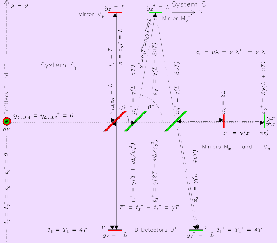
Fig. 3 : The Michelson–Morley experiment is outlined in the preferred System S_p by the red items emitter (radiating photons with an energy of $h\,\nu$ in its rest frame), beam splitter, mirrors and detector, if the apparatus in System S is at rest in S_p, as well as by green items moving relative to System S_p with a velocity $v$ parallel to the $x$-coordinate axes. The systems are assumed to coincide at $t_{0}=t^{+}_{0}=0$, when a photon in each of the systems is emitted. The propagation of the photons occurs in System S_p. Their paths are indicated by solid lines if $v=0$ and their energy is $E=h\,\nu$. If $v\neq 0$, dotted lines signal an energy $E^{+}=h\,\nu^{+}$, dashed-dotted lines an energy $E^{-}=h\,\nu^{-}$, and dashed lines $E=\gamma\,h\,\nu$. Further explanations are given in the text.

5.1 Operation in vacuum

In Fig. 3, the experimental setup in System S is shown both at rest in the preferred System S_p with red optical elements and moving with a speed $v=\beta\,c_{0}$ in the positive $x$-direction with green optical elements. The central beam splitter is shown twice at $[x^{+}_{1},t^{+}_{1}]$ and at $[x^{+}_{3},t^{+}_{3}]$, when it is hit by the photon. Photons are radiated by an emitter with energy $E=h\,\nu$, but if the emitter is moving with $v$, the photon energy in S_p is according to Eq. (19) $E^{+}=h\,\nu\,\sqrt{(1+\beta)/(1-\beta)}$ (dotted line). The receding mirror at $x^{+}_{5}$ induces the inverse Doppler effect twice (cf. Wilhelm & Fröhlich, 2013) leading to

$$E^{-}=h\,\nu\,\displaystyle{\sqrt{\frac{1+\beta}{1-\beta}}}\,\frac{1-\beta}{1+\beta}=h\,\nu\,\displaystyle{\sqrt{\frac{1-\beta}{1+\beta}}}~{},$$ (63)

shown by the dashed-dotted line.

The beam splitter at $x^{+}_{1}$, receding relative to the propagation direction of the photons, causes an inverse Doppler effect. The calculations at the end of Sect. 3 can be applied to this situation as follows: The photon is deflected in S by 90^o, but travels with $E=\gamma\,h\,\nu$ to Mirror M${}^{+}_{y}$ and Detector D⁺ (dashed lines) in S_p and, consequently, the magnitude of its momentum vector is $\gamma\,h\,\nu/c_{0}$. The momentum of the beam splitter changes parallel to the velocity by $-\beta\,\gamma\,h\,\nu/c_{0}$. Momentum conservation thus requires a momentum component of the photon parallel to $v$ of $\beta\,\gamma\,h\,\nu/c_{0}$. This yields together with its magnitude
$\cos\vartheta^{+}=(\beta\,\gamma\,h\,\nu/c_{0})/(\gamma\,h\,\nu/c_{0})=\beta$.

The beam splitter at $x^{+}_{3}$, advancing relative to the propagation direction of the photon, will cause a corresponding Doppler effect and aberration reflecting the photon also with $E=\gamma\,h\,\nu$ to Detector D⁺. However, only $h\,\nu$ will be absorbed, because the detector momentum change $\beta\,\gamma\,h\,\nu/c_{0}$ in $x$-direction has to be provided by the photon in addition to the fractional energy. With $\cos\vartheta^{+}=\beta$, the photon with an energy of $\gamma\,h\,\nu/c_{0}$ just fulfills these requirements.

Special mention should be made on the lengths of the inclined paths. The $y$-component is $s=c_{0}\,T$ and the $x$-component is $v\,(t^{+}_{2}-t^{+}_{1})=\beta\,\gamma\,c_{0}\,T$ thus

$$s^{+}=\sqrt{(c_{0}\,T)^{2}+(\beta\,\gamma\,c_{0}\,T)^{2}}=\gamma\,c_{0}\,T$$ (64)

is the geometric length in S_p. A consequence is that from $s=c_{0}\,T=q\,\lambda$ (cf. Fig. 1) it follows that $s^{+}=q\,\gamma\,\lambda$, confirming that the number $q$ is not dependent on the motion. Eq. (64) also shows that the total length of the light path between the positions of the beam splitter via the Mirror M${}^{+}_{y}$ is equal to the total length via the Mirror M${}^{+}_{x}$, namely
$2\,\gamma\,L=(x^{+}_{5}-x^{+}_{1})+(x^{+}_{5}-x^{+}_{3})$.
Finally, it should be noted that the times in both systems are related by $T^{+}=\gamma\,T$ according to Eq. (42).

All relations in Fig. 3 have been derived by momentum and energy conservation of the emitted, propagating and absorbed photons and optical elements. It is, however, important to note that they could have been obtained in the framework of STR with the Lorentz transformations in Eq. (42). For the Systems S and S_p in Fig. 3 the following relations result:

1. Emission of photon:
   $[x_{0},t_{0}]=[0,0]$
   $[x^{+}_{0},t^{+}_{0}]=[0,0]$

2. Position of beam splitter at first photon contact:
   $[x_{1},t_{1}]=[L,T]$
   $[x^{+}_{1},t^{+}_{1}]=[\gamma\,(L+v\,T),\gamma\,(T+v\,L/c^{2}_{0})]$

3. Position of mirror M${}^{+}_{y}$ at photon reflection:
   $[x_{2},t_{2}]=[L,2\,T]$
   $[x^{+}_{2},t^{+}_{2}]=[\gamma\,(L+2\,v\,T),\gamma\,(2\,T+v\,L/c^{2}_{0})]$

4. Position of beam splitter at second photon contact:
   $[x_{3},t_{3}]=[L,3\,T]$
   $[x^{+}_{3},t^{+}_{3}]=[\gamma\,(L+3\,v\,T),\gamma\,(3\,T+v\,L/c^{2}_{0})]$

5. Position of detector at photon detection:
   $[x_{4},t_{4}]=[L,4\,T]$
   $[x^{+}_{4},t^{+}_{4}]=[\gamma\,(L+4\,v\,T),\gamma\,(4\,T+v\,L/c^{2}_{0})]$

6. Position of mirror M${}^{+}_{x}$ at photon reflection:
   $[x_{5},t_{2}]=[2\,L,2\,T]$
   $[x^{+}_{5},t^{+}_{5}]=[2\,\gamma\,(L+v\,T),2\,\gamma\,(T+v\,L/c^{2}_{0})]$

5.2 Operation in air

Cahill & Kitto (2003) have claimed that the interferometer experiment of Michelson–Morley should give a null result only if operated under vacuum conditions. Brillet & Hall (2003) indeed obtained a null result in vacuum. Historic experiments performed by Michelson & Morley (1887) and Miller (1933), however, operated in air with an index of refraction at a wavelength of $\lambda=570$ nm of $n\approx 1.000\,2774$, which is only slightly depending on the atmospheric pressure. They did, in most cases, not produce exact null results.

In particular, Miller (1933) performed over decades many experiments with folded optical paths as long as 6406 cm, corresponding to a total light-path of $112\,000\,000\,\lambda$. He found a maximum displacement of $0.152\,\lambda$ and converted it to an “ether drift” of 11.2 km s^-1 Can the observations accounted for by measurement uncertainties as is generally done?

The propagation speed $c$ of light in a transparent body made out of a material with $n\neq 1$ moving with the speed $v$ relative to the observer was considered by Fresnel (1818) and Fizeau (1851, 1860) with the result that

$$c=\frac{c_{0}}{n}\pm v\left(1-\frac{1}{n^{2}}\right)~{},$$ (65)

where $(1-1/n^{2})$ is the so-called Fresnel aether drag coefficient, indicating a partial drag of the aether by the moving body. Fizeau (1851), however, was not convinced that these findings reflected the actual physical process:

1. ‘The success of the experiment seems to me to render the adoption of Fresnel’s hypothesis necessary, or at least the law which he found for the expression of the alteration of the velocity of light by the effect of motion of a body; for although that law being found true may be a very strong proof in favour of the hypothesis of which it is only a consequence, perhaps the conception of Fresnel may appear so extraordinary, and in some respects so difficult, to admit, that other proofs and a profound examination on the part of geometricians will still be necessary before adopting it as an expression of the real facts of the case.’ (cf. Comptes Rendus, Sept. 29, 1851)

More than 50 years later, von Laue (1907) found that the light can be assumed to be completely carried along by a body with $n\neq 1$, if the speeds $c=c_{0}/n$ and $v$ are combined according to the addition theorem of velocities. For parallel velocities $c$ and $v$, he obtained from Eq. (22) a speed of

$$w_{\parallel}^{\pm}=\frac{c\pm v}{1\pm\displaystyle{\frac{v}{c_{0}\,n}}}=c_{0}\,\frac{1\pm n\,\beta}{n\pm\beta}\approx\frac{c_{0}}{n}\pm v\left(1-\frac{1}{n^{2}}\right)~{},$$ (66)

where the approximation, valid for small $\beta$, is identical with Fresnel’s Eq. (65). If $v$ is perpendicular to $c$ in System S the theorem reads

$$w_{\perp}=\displaystyle{\sqrt{c^{2}+v^{2}\,\left(1-\frac{1}{n^{2}}\right)}}=\frac{c_{0}}{n}\,\sqrt{1+\beta^{2}\,(n^{2}-1)}~{}.$$ (67)

Without taking the velocity addition theorem into account, Cahill & Kitto (2003) deduced from Miller’s and other observations drift speeds of about 400 km s^-1 We feel, however, that the velocity addition theorem has to be applied in analysing the Michelson–Morley experiment. In air, the time $t_{1}$ is now $T=n\,L/c_{0}$ leading to the following relations:
The distance

$$\mathnormal{\Delta}x^{+}=x^{+}_{5}-x^{+}_{1}=\gamma\,\left(L+v\,n\,\frac{L}{c_{0}}\right)=\gamma\,L\,(1+n\,\beta)$$ (68)

is traversed in the time

$$\mathnormal{\Delta}t^{+}=\frac{\mathnormal{\Delta}x^{+}}{w_{\parallel}^{+}}=\gamma\,\frac{L}{c_{0}}\,(n+\beta)~{},$$ (69)

and in the reverse direction

$$\mathnormal{\Delta}x^{-}=x^{+}_{5}-x^{+}_{3}=\gamma\,\left(L-v\,n\,\frac{L}{c_{0}}\right)=\gamma\,L\,(1-n\,\beta)$$ (70)

in

$$\mathnormal{\Delta}t^{-}=\frac{\mathnormal{\Delta}x^{-}}{w_{\parallel}^{-}}=\gamma\,\frac{L}{c_{0}}\,(n-\beta)~{}.$$ (71)

The corresponding relations via $[x^{+}_{2},y^{+}_{2}]$ are: The distance from $[x^{+}_{1},y^{+}_{1}]$ to $[x^{+}_{3},y^{+}_{3}]$ was $\mathnormal{\Delta}y^{+}=2\,\gamma\,L$ in vacuum, but might be different with $n\neq 1$. So the task is to determine this distance. Several methods can be employed.

1. Since the length $L$ perpendicular to the velocity $v$ does not change, we can together with the distance
   $[x^{+}_{1},x^{+}_{2}]=\gamma\,v\,n\,T=\gamma\,\beta\,n\,L$ calculate with the help of Pythagoras’ theorem the length of the light path between the beam splitter and Mirror $y^{+}_{2}$ in System S_p:

   $$s^{+}_{n}=L\,\sqrt{1+\gamma^{2}\,\beta^{2}\,n^{2}}=\gamma\,L\,\sqrt{1+\beta^{2}\,(n^{2}-1)}~{}.$$ (72)

   The distance to $[x^{+}_{3},y^{+}_{3}]$ then is $2\,s^{+}_{n}$.

2. With Eq. (67) and $v$ we can find

   $$\cos\vartheta^{+}_{n}=\frac{n}{c_{0}}\,\frac{v}{\sqrt{1+\beta^{2}\,(n^{2}-1)}}~{},$$ (73)

   where $\vartheta^{+}_{n}$ is the angle $\vartheta^{+}$ in Fig. 3 for an operation in air. Again we get:

   $$s^{+}_{n}=\frac{\gamma\,\beta\,n\,L}{\cos\vartheta^{+}_{n}}=\gamma\,L\,\sqrt{1+\beta^{2}\,(n^{2}-1)}~{}.$$ (74)

3. She, Yu & Feng (2008) have recently shown that their experiment supports Abraham’s concept of a momentum of light in media with $n\neq 1$ proportional to $1/n$. Since in our case the emitter, the beam splitter and the air are moving together with speed $v$ relative to S_p, a photon will be radiated perpendicular to $v$ with energy $h\,\nu$ and momentum $h\,\nu/(n\,c_{0})$ under the assumption of no recoil. From Eqs. (9) and (10) and the conservation of energy and the $x$-component of the momentum, we get

   $$\tan\vartheta^{+}_{n}=\frac{\displaystyle{\frac{h\,\nu}{n\,c_{0}}}}{\displaystyle{\frac{\gamma\,h\,\nu\,\beta}{c_{0}}}}=\frac{1}{\gamma\,n\,\beta}$$ (75)

   and with $\tan\vartheta^{+}_{n}=\sin\vartheta^{+}_{n}/\cos\vartheta^{+}_{n}$

   $$\cos\vartheta^{+}_{n}=\frac{n}{c_{0}}\,\frac{v}{\sqrt{1+\beta^{2}\,(n^{2}-1)}}~{},$$ (76)

   the same result as in b).

Invoking all the three methods, we thus obtain

$$2\,s^{+}_{n}=2\,\gamma\,L\,\sqrt{1+\beta^{2}\,(n^{2}-1)}$$ (77)

and

$$\mathnormal{\Delta}t_{\perp}=\frac{2\,s^{+}_{n}}{w_{\perp}}=\frac{2\,\gamma\,L\,\sqrt{1+\beta^{2}\,(n^{2}-1)}}{\displaystyle{\frac{c_{0}}{n}\,\sqrt{1+\beta^{2}\,(n^{2}-1)}}}=\frac{2\,n\,\gamma\,L}{c_{0}}~{}.$$ (78)

We can now calculate for the different arms of the interferometer

$$\mathnormal{\Delta}t^{+}+\mathnormal{\Delta}t^{-}-\mathnormal{\Delta}t_{\perp}=0$$ (79)

and find that there is no delay. It therefore appears as if Cahill’s and Kitto’s claim is not supported assuming von Laue’s drag velocities.

6 Discussion and conclusion

An aether concept – required by GTR (Einstein, 1924) – is not inconsistent with STR, and allows us to interpret the photon processes on the basis of momentum and energy conservation. A determination of the speed of a laboratory system relative to the aether does, however, not seem to be possible, i.e., neither with operation in vacuum nor in air.

Appendix A Derivation of the relativistic Doppler effect

The evaluation of Eq. (17) using Eqs. (8) to (11) can be achieved as follows:

$$(E^{*})^{2}-2\,E^{*}h\,\nu^{\pm}+(h\,\nu^{\pm})^{2}=m^{2}\,c^{4}_{0}+(p^{\pm})^{2}c^{2}_{0}=$$

$$m^{2}\,c^{4}_{0}+(p^{*})^{2}c^{2}_{0}\mp 2\,p^{*}\,c_{0}\,h\,\nu^{\pm}+(h\,\nu^{\pm})^{2}=m^{2}\,c^{4}_{0}+(E^{*})^{2}\,\beta^{2}\mp 2\,\beta\,E^{*}\,h\,\nu\pm+(h\,\nu^{\pm})^{2}~{}.$$ (A1)

Deletion of $(h\,\nu^{\pm})^{2}$ from the first and last lines gives:

$$(E^{*})^{2}-2\,E^{*}h\,\nu^{\pm}=m^{2}\,c^{4}_{0}+(E^{*})^{2}\,\beta^{2}\mp 2\,\beta\,E^{*}\,h\,\nu^{\pm}~{}.$$

and

$$(E^{*})^{2}\,(1-\beta^{2})-2\,E^{*}\,h\,\nu^{\pm}\,(1\mp\beta)=m^{2}\,c^{4}_{0}~{}.$$ (A2)

Substituting finally $E^{*}$ results in

$$\mathnormal{\Delta}E\,(m\,c^{2}_{0}+\mathnormal{\Delta}E/2)=\gamma\,(m\,c^{2}_{0}+\mathnormal{\Delta}E)\,h\,\nu^{\pm}\,(1\mp\beta)$$ (A3)

after deletion of $m^{2}\,c^{4}_{0}$ on both sides and noting that
$\gamma^{2}=1/(1-\beta^{2})$. With $\mathnormal{\Delta}E=h\,\nu$ in the emitter system the relativistic Doppler formula follows.

References

- Abraham (1903) Abraham, M., 1903, Prinzipien der Dynamik des Elektrons, Ann. Phys. (Leipzig), 310, 501
- Audoin & Guinot (2001) Audoin, C., Guinot, B., 2001, The measurement of time. Time, frequency and atomic clock, Cambridge University Press, Cambridge
- Bradley (1727) Bradley, J., 1727, A letter from the Reverend Mr. James Bradley Savilian Professor of Astronomy at Oxford, and F.R.S. to Dr. Edmond Halley Astronom. Reg. &c. giving an account of a new discovered motion of the fix’d stars, Phil. Trans., 35, 637
- Brillet & Hall (2003) Brillet, A., Hall, J. L., 1979, Improved laser test of the isotropy of space, Phys. Rev. Lett. 42, 549
- Builder (1958) Builder, G., 1958, Ether and relativity, Austr. J. Phys., 11, 279
- BIPM (2006) Bureau international des poids et mesures (BIPM), 2006, Le systéme international d’unités (SI), 8e édition
- Cahill & Kitto (2003) Cahill R. T., Kitto K., 2003, Michelson–Morley experiments revisited and the Cosmic Background Radiation preferred frame, Apeiron, 10, 104
- Dirac (1936) Dirac, P. A. M., 1936, Relativistic wave equations, Proc. Roy. Soc. Lond. A, 155, 447
- Dirac (1951) Dirac, P. A. M., 1951, Is there an æther? Nature, 168, 906
- Doppler (1842) Doppler, C., 1842, Ueber das farbige Licht der Doppelsterne und einiger anderer Gestirne des Himmels, Abh. k. b hm. Ges. Wiss., V. Folge, Bd. 2, 465
- Eddington (1923) Eddington, A. S., 1923, Can gravitation be explained? J. Roy. Astron. Soc. Can., 17, 387
- Einstein (1905a) Einstein, A., 1905a, Über einen die Erzeugung und Verwandlung des Lichtes betreffenden heuristischen Gesichtspunkt, Ann. Phys. (Leipzig), 322, 132
- Einstein (1905b) Einstein, A., 1905b, Zur Elektrodynamik bewegter Körper, Ann. Phys. (Leipzig), 322, 891
- Einstein (1905c) Einstein, A., 1905c, Ist die Trägheit eines Körpers von seinem Energieinhalt abhängig? Ann. Phys. (Leipzig), 323, 639
- Einstein (1907) Einstein, A., 1907, Über die Möglichkeit einer neuen Prüfung des Relativitätsprinzips, Ann. Phys. (Leipzig), 328, 197
- Einstein (1908) Einstein, A., 1908, Über das Relativitätsprinzip und die aus demselben gezogenen Folgerungen, Jahrbuch der Radioaktivität und Elektronik 1907, 4, 411
- Einstein (1920) Einstein, A., 1920, Äther und Relativitätstheorie, Rede gehalten am 5. Mai 1920 an der Reichs-Universität zu Leiden, Berlin, Verlag von Julius Springer
- Einstein (1924) Einstein, A., 1924, Über den Äther, Verhandl. Schweiz. Naturforsch. Gesell., 105, 85
- Einstein (1917) Einstein, A., 1927, Zur Quantentheorie der Strahlung, Phys. Z. XVIII, 121
- Fermi (1932) Fermi, E., 1932, Quantum theory of radiation, Rev. Mod. Phys., 4, 87
- Fizeau (1851) Fizeau, H., 1851, The hypotheses relating to the luminous æther, and an experiment which appears to demonstrate that the motion of bodies alters the velocity with which light propagates itself in their interior, Phil. Mag., Series 4, 2, 568
- Fizeau (1860) Fizeau, H., 1860, On the effect of the motion of a body upon the velocity with which it is traversed by light, Phil. Mag., Series 4, 19, 245
- Fresnel (1818) Fresnel, A., 1818, Lettre d’Augustin Fresnel á François Arago sur l’influence du mouvement terrestre dans quelques phénomènes d’optique, Ann. Chim. Phys. 9, 57
- Granek (2001) Granek, G., 2001, Einstein’s ether: F. Why did Einstein come back to the ether? Apeiron, 8, 19
- Ives and Stilwell (1938) Ives, H. E., Stilwell, G. R., 1938, An experimental study of the rate of a moving atomic clock, J. Opt. Soc. Am., 28, 215
- Ives and Stilwell (1941) Ives, H. E., Stilwell, G. R., 1941, An experimental study of the rate of a moving atomic clock II., J. Opt. Soc. Am., 31, 369
- Jackson (2001) Jackson, J. D., 2001, Klassische Elektrodynamik, 4. Aufl., Walter de Gruyter, Berlin, New York
- Kostro (2004) Kostro, L., 2004, Albert Einstein’s new ether and his general relativity, Conf. Appl. Differential Geometry, 2001 (Ed. G. Tsagas) Balkan Press, pp. 78–86
- Kragh and Overduin (2014) Kragh, H. S., Overduin, J., 2014, The weight of the vacuum. A scientific history of Dark Energy, Springer, ISBN: 978-3-642-55089-8
- von Laue (1907) von Laue, M., 1907, Die Mitführung des Lichtes durch bewegte Körper nach dem Relativitätsprinzip, Ann. Phys., 328, 989
- von Laue (1908) von Laue, M., 1908, Die Wellenstrahlung einer bewegten Punktladung nach dem Relativitätsprinzip, Verhandl. Deutsche Physikal. Ges., 10, 838
- von Laue (1912) von Laue, M., 1912, Zwei Einwände gegen die Relativitätstheorie und ihre Widerlegung, Phys. Z., XIII, 118
- von Laue (1920) von Laue, M., 1920, Zur Theorie der Rotverschiebung der Spektrallinien an der Sonne, Z. Phys., 3, 389
- von Laue (1921) von Laue, M., 1921, Die Lorentz-Kontraktion, Philosophische Zeitschrift, 26, 91
- von Laue (1959) von Laue, M., 1959, Geschichte der Physik, 4. erw. Aufl., Ullstein Taschenbücher-Verlag, Frankfurt/Main
- Lewis (1926) Lewis, G. N., 1926, The conservation of photons, Nature, 118, 874
- Lorentz (1895) Lorentz, H. A., 1895, Versuch einer Theorie der electrischen und optischen Erscheinungen in bewegten Körpern, E.J. Brill, Leiden
- Lorentz (1904) Lorentz, H. A., 1903, Electromagnetic phenomena in a system moving with any velocity smaller than that of light, Koninkl. Nederl. Akad. Wetensch. Proc., 6, 809
- Mermin (1984) Mermin, N. D., 1984, Relativity without light, Am. J. Phys., 52, 119
- Michelson & Morley (1887) Michelson, A. A., Morley, E. W., 1887, On the relative motion of the Earth and of the luminiferous Ether, Sidereal Messenger, 6, 306
- Michelson et al. (1928) Michelson, A. A. Lorentz, H. A., Miller, D. C., Kennedy, R. J., Hedrick, E. R., Epstein, P. S., 1928, Conference on the Michelson–Morley experiment held at Mount Wilson, February, 1927, Astrophys. J. 68, 341
- Miller (1933) Miller, D. C., 1933, The ether-drift experiment and the determination of the absolute motion of the Earth, Rev. Mod. Phys., 5, 203
- Mössbauer (1958) Mössbauer, R. L., 1958, Kernresonanzfluoreszenz von Gammastrahlung in Ir191, Z. Physik., 151, 124
- Poincaré (1900) Poincaré, H., 1900, La théorie de Lorentz et le principe de réaction, Arch. Néerland. Sci. exact. natur., 5, 252
- Poincaré (1905) Poincaré, H., 1905, Sur la dynamique de l’électron, Compt. Rend., 140, 1504
- Okun (1989) Okun, L. B., 1989, The concept of mass, Phys. Today, 42 (60), 31
- Saathoff et al. (2011) Saathoff, G., Reinhardt, S., Bernhardt, B., 16 co-authors, 2011, Testing time dilation on fast ion beams, CPT AND Lorentz Symmetry. (Ed. V. Alan Kosteleck ) World Scientific Publishing Co., pp. 118–122
- Schröder (1990) Schröder, W., 1990, Ein Beitrag zur frühen Diskussion um den Äther und die Einsteinsche Relativitätstheorie, Ann. Phys. 7. Folge, 326, 6, 475
- She, Yu & Feng (2008) She, W., Yu, J., Feng, R., 2008, Observation of a push force on the end face of a nanometer silica filament exerted by outgoing light, Phys. Rev. Lett. 101, 243601
- Smoot et al. (1991) Smoot, G. F., Bennett, C. L., Kogut, A., 25 co-authors, 1991, Preliminary results from the COBE differential microwave radiometers – Large angular scale isotropy of the cosmic microwave background, Astrophys. J., Part 2, 371, L1
- Stark (1907) Stark, J., 1907, Über die Lichtemission der Kanalstrahlen in Wasserstoff, Ann. Phys. (Leipzig), 326, 401
- Wiechert (1911) Wiechert, E., 1911, Relativitätsprinzip und Äther, Phys. Z., 12, 689 & 758
- Wilhelm & Fröhlich (2013) Wilhelm, K., Fröhlich, C., 2013, Photons – from source to detector, in Observing Photons in Space (eds. M. C. E. Huber et al.), Springer, New York, Heidelberg, Dordrecht, London, pp. 21–53