Uncertainty Estimates for Theoretical Atomic and Molecular Data

Abstract

Sources of uncertainty are reviewed for calculated atomic and molecular data that are important for plasma modeling: atomic and molecular structure and cross sections for electron-atom, electron-molecule, and heavy particle collisions. We concentrate on model uncertainties due to approximations to the fundamental many-body quantum mechanical equations and we aim to provide guidelines to estimate uncertainties as a routine part of computations of data for structure and scattering.

I Introduction

There is growing acceptance that benchmark atomic and molecular (A+M) calculations should follow accepted experimental practice and include an uncertainty estimate alongside any numerical values presented The Editors (2011). Increasingly, A+M computations are also being used as the primary source of data for input into modeling codes. It is our assertion that these data should, if at all possible, also be accompanied by estimated uncertainties. However, it is not at all straightforward to assess the uncertainties associated with A+M computations. The aim of this work is to provide guidelines for A+M theorists to acquire uncertainty estimates as a routine part of their work. We concentrate on data that are most important for high-temperature plasma modeling: data for A+M structure, electron-atom (or ion) collisions, electron collisions with small molecules, and charge transfer in ion-atom collisions.

Uncertainty Quantification (UQ) is a very active research area in connection with simulations of complex systems arising in weather and climate modeling, simulations of nuclear reactors, radiation hydrodynamics, materials science, and many other applications in science and engineering. A report from the USA National Research Council National Research Council Committee on Mathematical Foundations of Verification, Validation, and Uncertainty Quantification (2012) provides a valuable survey. The current state of the field is reflected in the biennial meeting of the SIAM Activity Group on Uncertainty Quantification SIA . This field of UQ for complex systems has a mathematical core in the description of uncertainty propagation for chaotic deterministic and stochastic evolution equations in many dimensions (“polynomial chaos”). In many cases the interest is then focused on systems for which the basic equations are not well established and involve poorly known parameters and functional dependencies.

The present article is concerned with quantification of uncertainties in elaborate computations, but the nature of computational A+M science for application to high temperature plasmas is rather different from the focus areas of present UQ science. This A+M science is concerned with simple physical systems and their interactions. The underlying equations governing the processes of interest and the ensuing dynamics are essentially known Dirac (1929), but except for a few special cases a true first-principles treatment is numerically intractable: the complexity scales exponentially with the number of electrons while for a fixed number of electrons the complexity of the first-principles equations using a basis tends to scale polynomially in the basis size with the number of electrons in the exponent. A+M theory is, therefore, about development of models that aim to approximate the exact problem with numerically tractable procedures. The uncertainties in these procedures, referred to as “model uncertainties” in the following, are strongly model-dependent and are often poorly understood. The solution of any given model is itself subject to uncertainties due to convergence and other numerical issues associated with a grid or a basis set. These will be referred to as “numerical uncertainties”. Finally, closer to established UQ science, uncertainties propagate through the various stages of a calculation, e.g., from structure to collisions, in ways that are hard to quantify.

Plasma conditions in, for example, astrophysics and nuclear fusion applications span many orders of magnitude variation in energy and in spatial and temporal scales, and systems can be far from thermodynamic equilibrium. Basic data may be required for quite strange-looking A+M systems; e.g., for collision processes between neutral atoms and highly charged ions (relevant for neutral beam heating in fusion plasma and for processes involving the solar wind) or for neutral and low charge states of atoms in high temperature plasma (relevant for laser-produced plasma and for plasma-wall interaction). For applications to low-temperature industrial plasmas, similar to the case of chemical dynamics, data are required for transient species such as molecular radicals and molecular complexes above the dissociation threshold. In addition, for applications in plasma chemistry essentially always data are required for multiple electronic states, corresponding to the possibility of charge transfer. Very often the modeling requires data that are not accessible to direct experiments; for example, data for atomic processes from excited initial states, data for molecular processes resolved with respect to the rovibrational state of the molecule, data for processes involving electronically excited molecules, data for molecular radicals, and to some extent data involving hazardous species such as tritium or beryllium.

To develop an effective and objective science of uncertainty assessment for A+M applications one has to bring together physics, chemistry, computer science, and applied mathematics communities. The A+M and plasma modeling communities are making the first steps in this direction, for example by meetings such as IAE (2014) and Sto (2015). Our ultimate goal is to develop guidelines for self-validation of computational theory for A+M processes; i.e.  computational procedures by which an uncertainty estimate is obtained along with the primary quantity of interest. We recognize that experimental benchmark data are sometimes available and can be used for additional validation. In general, this is more readily possible for structural studies (where spectroscopic data often provide benchmark accuracy) than for studies of collision processes. Similarly, procedures for uncertainty estimates are currently better developed for structure calculations than for scattering. This will be further elaborated below.

Energies and state-resolved cross sections are the primary data from A+M science, but these data are normally processed further before being used in plasma modeling codes, which tend to use effective rate coefficients for processes in thermal plasma with explicit account of long-lived electronic states only. The processed data may be tabulated for interpolation or fit functions may be used, or a combination of interpolation and function fitting. At that stage completeness of the data (relative to processes covered and range of collision energy) and qualitative correctness of behavior at extreme conditions is essential; more important than pointwise accuracy. These processed, tabulated and fitted data are incorporated into integrated modeling codes, and a key challenge for theory and simulation is the consistent integration of all processes and scales together with a well-founded assessment of uncertainties as they are generated and propagated in the simulations. For the propagation of uncertainties in A+M data through a simple plasma model (no spatial dependence) we note the HydKin toolkit Reiter and Janev (2010), which has been developed to support fusion plasma modeling and other applications.

The focus of the present work is on calculations based on quantum mechanics for A+M properties and processes that are important in plasmas: atomic and molecular structure, electron collisions with atoms and molecules (and their ions), and charge transfer in ion-atom and ion-molecule collisions. Processes governed by time-dependent fields and photon-induced processes are not considered. Section II contains general remarks about the need for uncertainty estimates and about approaches for uncertainty assessment. In section III we discuss uncertainty assessment for atomic and molecular electronic structure. Section IV is concerned with uncertainty assessment for electron-atom and electron-molecule collisions. In section V we consider charge transfer in heavy particle collisions. Section VI is concerned with uncertainty assessment in practice, with examples from atomic and molecular structure, electron collisions and heavy particle collisions. In section VII we provide conclusions and an outlook for future work.

II General Considerations

Uncertainties should be provided for observable and other physically important intermediate quantities, such as molecular electronic excitation energies. Quantities in structural studies for which uncertainties should routinely be provided include:

• energy level differences, such as excitation and ionization energies and for molecules also dissociation energies and barrier heights;

• configurational parameters of molecules such as bond lengths and bond angles at local minima and transition states;

• properties, such as dipole moments, oscillator strengths, lifetimes, and polarizabilities;

• numerical issues such as analytical representations (fits) yielding potential energy and dipole moment surfaces.

Quantities in collisional studies for which uncertainties should routinely be provided include:

• threshold energies;

• cross sections and/or appropriate rates;

• positions and widths of key resonances;

• other observables, such as the polarization of the emitted radiation, branching ratios, etc..

It may also be desirable to provide uncertainties for other key computed quantities, such as eigenphase sums or scattering lengths, which are important for the theoretical analysis of given processes. These quantities, however, do not generally form input of modeling codes and therefore the provision of uncertainties can be regarded as having lower significance. It must be recognized that there are difficulties in estimating uncertainties in some cases, for example if a resonance comes out on the wrong side of a threshold. This observation means that a computational model must have reached a sufficient level of stability and accuracy before an uncertainty estimate is appropriate. However it is exactly such computations that provide benchmarks and inputs to modeling codes.

For structural studies, including computations of relative energies and properties, the focal point analysis (FPA) technique Császár et al. (1998) provides an excellent procedure to assign uncertainties for key quantities. Studies building on an FPA approach can also include uncertainty estimates for effects not explicitly computed: for example it is much easier to estimate the magnitude of higher order electron correlation or nonadiabatic corrections to the Born-Oppenheimer approximation than it is to compute them in specific cases; see Boyarkin et al. (2013) for example.

In clear contrast, at present there is no well-defined general procedure for uncertainty propagation in scattering calculations. Notable exceptions are the way uncertainties in dipole moments and oscillator strengths propagate from structure to certain collisional observables.

It is important to estimate all major corrections separately, rather than as a sum that may contain accidental cancellations, and to compare the estimates with known values for reference ions. Whenever possible, calculations should be done by more than one method (such as CI and MCHF), and the results compared for consistency. In the ideal scenario, for a given method of calculation, uncertainties in the parameters of the method should be propagated towards uncertainties in the final results (cross sections, energies, etc.). Due to the need to approximate the many-electron Schrödinger equation with a tractable model, systematic errors are in general unavoidable. The use of different independent methods will help to reduce the influence of systematic unknown errors. Assuming that some uncertainty estimate is available the results from different methods can be combined using a Bayesian approach to produce a final probability distribution for quantities of interest, from which a revised uncertainty can be obtained. The use of models in combination with experimental benchmarks to produce correlated probability distributions for quantities of interest has become rather well established in the nuclear data community under names such as Total Monte Carlo (TMC) or Unified Monte Carlo (UMC); for example see Ref.  berto Capote and Smith (2008). It would be very interesting to see such a formal and objective approach applied in the field of atomic, molecular and optical physics as well.

Once the evaluation (comparison) between results of theoretical methods is done, the final step is to check that the uncertainty estimates are in accord with the actual differences between theory and experiment for known cases. For an objective evaluation, in an ideal situation, when experimental and theoretical uncertainties are available, the same evaluation procedure based on the formal statistical approach is recommended. The data (values and uncertainties) resulted from this evaluation would account for all available information from theory and experiment. If no systematic error in the theoretical data is suspected (for example, if two different methods produce results within their intervals of uncertainties), the theoretical results and their uncertainties could be extended to cases where there are no experimental data available.

The above discussion demonstrates why uncertainty quantification is very important in theoretical calculations. Unfortunately, uncertainty quantification of the final results from a given theoretical method is often impossible or very difficult. But it is still strongly recommended that the authors of the produced data give an approximate estimate of uncertainty of the produced results for the purposes discussed above. In many situations, where the direct uncertainty propagation is not possible, sensitivity tests could and should be performed to collect statistics and estimate uncertainties of the final results.

III Uncertainty Estimates for Structure Computations

III.1 Atoms

The discussion of uncertainties in atomic structure computations begins with one- and two-electron atoms and ions since these provide the traditional testing grounds for theory in comparison with experiment. Theoretical uncertainties here limit the accuracy that can be achieved for more complex atomic systems.

The highest accuracy can of course be achieved for hydrogen and other two-body problems since the Schrödinger equation can be solved exactly to find the exact nonrelativistic wave function and energy Bethe and Salpeter (1957). Uncertainties then come from relativistic and quantum electrodynamic (QED) corrections, and the effects of finite nuclear size and structure (for a general review, see ref. Eides et al. (2001)). The sizes of the relativistic and QED corrections are determined by the dual expansion parameters $\alpha$ and $\alpha Z$, where $\alpha=1/137.035999139(31)$ is the fine structure constant and $Z$ is the nuclear charge Jentschura et al. (2005). Beginning with the lowest order nonrelativistic energy, the relativistic corrections can generally be represented as an expansion in powers of $(\alpha Z)^{2}$. For the case of one-electron atoms and infinite nuclear mass, the series can be summed to infinity by solving instead the Dirac equation to obtain the exact relativistic energies Bethe and Salpeter (1957). However, QED corrections (Lamb shifts) cannot be similarly summed to all orders, and so represent a dominant source of uncertainty. The lowest order one-loop terms from vacuum polarization and electron self-energy are of order $\alpha^{3}Z^{4}$ Ry. These can be calculated essentially exactly. Higher order terms come from both binding energy corrections as additional powers of $\alpha Z$, and multi-loop Feynman diagrams as additional powers of $\alpha$. The higher order terms are known in their entirety up to $\alpha^{6}Z^{6}$ Ry, but the uncertainty in the numerical coefficients gives an uncertainty of order $\alpha^{6}Z^{7}$ Ry, or a few kHz for the ground state of hydrogen Pachucki and Jentschura (2003). The uncertainty from finite nuclear size effects is about an order of magnitude larger, and hence dominates.

For heavy hydrogenic ions up to U⁹¹⁺ and beyond, considerable progress has been made in summing the binding energy corrections (i.e. powers of $\alpha Z$) to all orders for certain classes of diagrams Yerokhin and Shabaev (2015), coupled with experiments for comparison (see Gumberidze et al. Gumberidze et al. (2011), and earlier references therein). For the ground state of U⁹¹⁺, the theoretical Lamb shift is $464.26\pm 0.5$ eV, in good agreement with the measured value $460.2\pm 4.6$ eV. For excited s-states, the Lamb shifts and uncertainties scale approximately as $1/n^{3}$ with $n$ and $Z^{6}$ with $Z$. These uncertainties place a fundamental limit on the accuracy of atomic structure computations.

For atoms or ions containing two or more electrons, the Schrödinger equation is not separable, and hence cannot be solved exactly. Electron correlation then enters as an important new source of uncertainty. The correlation energy represents the difference between the exact energy, and the Hartree-Fock (HF) approximation arising from the use of spherically averaged potentials to obtain an independent particle approximation. Methods for few-electron atoms are divided into two broad categories, depending on the relative importance of correlation effects and relativistic corrections. As a function of $Z$ for an isoelectronic sequence, correlation effects are proportional to $Z^{0}=1$ (i.e. a constant) while the lowest order relativistic corrections are proportional to $\alpha^{2}Z^{3}$. There is therefore a crossover point when $\alpha^{2}Z^{3}=1$, or $Z=1/\alpha^{2/3}\simeq 27$. For $Z\leq 27$, correlation effects dominate relativistic effects. Consequently, one should start with the best possible solutions to the nonrelativistic Schrödinger equation and treat relativistic corrections as a perturbation. Conversely, when $Z>27$, one should start with exact one-electron solutions to the Dirac equation, and treat electron correlation as a perturbation. We will call these two regions the low-$Z$ and high-$Z$ regions respectively. There is a broad region around $Z=27$ where both methods yield useful results, and provide interesting comparisons to assess the accuracy.

Atoms with two or three electrons provide a special case because specialized techniques are available that yield essentially exact solutions to the Schrödinger equation. This is achieved by expanding the wave function in a Hylleraas basis set of functions involving explicitly powers of the interelectron coordinate $r_{12}=|{\bf r}_{1}-{\bf r}_{2}|$, where ${\bf r}_{1}$ and ${\bf r}_{2}$ are the position vectors of the individual electrons. Since a Hylleraas basis set is provably complete Klahn and Bingel (1977, 1978), a variational calculation in Hylleraas coordinates is guaranteed to converge from above to the exact nonrelativistic energy. The accuracy can be readily determined from the rate of convergence as more functions are added to the basis set. In this way, the nonrelativistic energy of the ground state of helium has been determined to 35 or more significant figures Schwartz (2006); Nakashima and Nakatsuji (2007), and results accurate to 20 or more significant figures can be readily obtained for the entire singly excited spectrum of helium Drake and Yan (1992). At this level of accuracy, calculations must be done in at least quadruple precision (32 decimal digits). Some authors go even further to use multiple precision arithmetic (48 or 64 decimal digits) Korobov (2000); Bailey (1993, 1995) in order to avoid numerical linear dependence in the basis set and preserve numerical stability. The record is the 101-digit arithmetic used by Schwartz Schwartz (2006) for the ground state of helium. However, the standard quadruple precision arithmetic provided by FORTRAN is usually sufficient, provided that care is exercised in choosing the basis set in order to avoid excessive numerical linear dependence. See for example Ref. Drake et al. (2002) for the use of triple basis sets in Hylleraas coordinates to maintain numerical stability. Results for lithium-like atoms with three electrons are not as accurate because the basis sets become considerably larger (i.e. 30,000 terms instead of 3,000 terms), but energies accurate to 16 figures and other atomic properties can still readily be obtained Wang et al. (2012).

At these levels of accuracy for two- and three-electron atoms, the dominant sources of uncertainty in the low-$Z$ region are the relativistic and QED corrections, as discussed above for hydrogen. The Breit interaction accounts for relativistic corrections of order $\alpha^{2}Z^{4}$ Ry, and a full many-electron theory accounts completely for QED corrections of order $\alpha^{3}Z^{4}$ (including the Araki-Sucher terms for QED corrections to the electron-electron interaction) Drake and Martin (1998); Morton et al. (2006); Yan et al. (2008a). Theory has also recently been completed for all terms of order $\alpha^{4}Z^{5}$ Ry Yerokhin and Pachucki (2010), although the nonrelativistic operators become complicated and difficult to evaluate. The resulting uncertainty from higher order terms is estimated to be 36 MHz for the ionization energy of the ground state of helium, and this scales as $Z^{5}$ with nuclear charge and roughly $1/n^{3}$ with $n$. For a comprehensive review, and tabulation for all states up to $n=10$ and angular momentum $L=7$, see ref. Drake (2006).

In the high-$Z$ region, the all-orders methods described above for hydrogenic ions can be extended to helium-like ions and combined with $1/Z$ expansion calculations from the low-$Z$ region (the so-called unified method) to obtain results that are accurate over the entire range from $Z=2$ to $Z=100$ Drake (1988); Artemyev et al. (2005). In most cases, the theoretical accuracy is better than the experimental. The uncertainty from omitted terms of order $\alpha^{4}Z^{4}$ is estimated to be $\pm$1.2$(Z/10)^{4}$ cm^-1 for the $n=2$ states.

Calculations of similar accuracy can also be carried out in Hylleraas coordinates for three-electron atoms, but that is the limit to what has been achieved to date. Further progress is hindered by the technical difficulties of calculating integrals involving nonseparable products of factors containing all the interelectron coordinate of the form $r_{12}r_{23}r_{34}\cdots$.

For many-electron atoms, one must resort instead to generally applicable methods of atomic structure based on the HF approximation, or its generalizations to the multi-configuration Hartree-Fock (MCHF) or configuration interaction (CI) methods. The MCHF method is usually called MCSCF in quantum chemistry as the HF approximation is called the self-consistent field (SCF) method. The relativistic versions of these methods are based on the Dirac equation instead of the Schrödinger equation, and are called the Dirac-Fock (DF) approximation, with generalizations to the corresponding multi-configuration Dirac-Fock (MCDF) or relativistic configuration interaction (RCI) methods. The basic approximation of the HF and DF methods is to assume that the many-electron wave function can be written as an antisymmetrized product of one-electron orbitals (a Slater determinant). The HF (or DF) solution is the one that minimizes the energy over all wave functions that can be expressed in this Slater determinant form. The difference between the HF (or DF) energy and the exact energy is called the electron correlation energy. The correlation energy can be systematically taken into account by solving a larger problem in which the mixing with other electronic configurations is included. The configuration mixing is induced by the difference between the effective HF potential and the exact electrostatic potential containing all the interelectronic repulsion terms. The difference between CI and MCHF revolves around whether or not the electron orbitals are frozen (CI) or allowed to vary (MCHF) to obtain a self-consistent solution. The correlation energy is of key importance in chemical physics, because it is typically the same order of magnitude (about 1 eV) as chemical binding energies. One might say that much of chemistry is buried in the correlation energy. Full spectroscopic accuracy can require correlation energies as accurate as $\pm$$10^{-9}$ eV or better for neutral atoms.

The coupled cluster (CC) method is a variation of CI, which also starts from the HF orbitals, but then uses Brueckner-Goldstone perturbation theory to describe excitations from the HF reference state, organized as singles (S), doubles (D), triples (T) etc. The advantage is that it guarantees the size-extensivity of the solution, but it lacks the variational character of the CI method.

Both the CI and MCHF methods are exact in principle (within their respective nonrelativistic or relativistic approximations) and generally applicable to many-electron atoms and ions, but they are much more slowly convergent than the methods based on Hylleraas basis sets for two- or three-electron atoms. It can be shown that a CI calculation is equivalent to a Hylleraas calculation that includes only the even powers of $r_{12}$ in the basis set, but it is the odd powers that are most effective in reproducing the cusp at $r_{12}=0$ in the correlated electronic wave function. For this reason, a CI calculation requires much larger numbers of configurations in the variational wave function in order to achieve even modest levels of accuracy, and so careful convergence studies must be carried out to assess the uncertainty in the calculation. Convergence uncertainties better than $\pm$$10^{-6}$ eV are seldom achieved, even for few-electron atoms, and the convergence is typically much worse for many-electron atoms. For example, Chantler et al Chantler et al. (2010) carried out a detailed convergence study for satellite spectra of the copper $K$-alpha photo-emission spectrum, and found that uncertainties were of the order of $\pm$$0.01-0.1$ eV using the MCDF method. Their work includes a detailed consideration of valence-valence and valence-core contributions to the correlation energy. They also make use of comparisons between the length and velocity forms of dipole transition integrals to assess the accuracy. Many other similar studies have been carried out. A great deal of work has now been done by many authors to develop systematic procedures to assess the theoretical/computational uncertainties, and to assign reasonable uncertainty estimates Fischer (2014); Träbert (2014); Kramida (2014); Ekman et al. (2014); Kelleher (2014); Safronova et al. (2014a, b); Kállay et al. (2011). Uncertainties of transition parameters can be evaluated by investigating differences between results calculated in the length and the velocity gauges for $LS$-allowed transitions Fischer (2009), and the analysis can be also extended for $LS$ intercombination lines for certain cases Ekman et al. (2014). Perturbative analysis by performing smaller calculations with neglected correlation effects is also useful to estimate uncertainties Fischer (2014).

Furthermore, it is necessary to include uncertainties due to physical effects not included in the calculation, such as additional classes of excitations, or quantum electrodynamic corrections. In recent work authors such as Safronova et al. Safronova et al. (2014a) and Kállay et al. Kállay et al. (2011) have made progress towards a comprehensive programme for the assessment of uncertainties that goes beyond the simple assessment of convergence uncertainties. The objective is to estimate an uncertainty that is independent of the actual difference between theory and experiment. For uncertainties of this type, the central value is not necessarily the most probable. For example, if QED corrections of order $\alpha^{3}$ have been omitted, then one can expect further corrections of order $\pm$$c\alpha^{3}$, where $c$ is a nonzero coefficient whose value can often be estimated from other similar calculations, or from general scaling rules with $n$ and $Z$. It is often possible to establish similar “reference ions” where experimental data exist for comparison with theoretical estimates of the uncertainties. The aim is to obtain reasonable estimates of the uncertainties, not rigorous bounds on the actual difference between theory and experiment (i.e. the error).

III.2 Molecular electronic ground state properties

Without the so-called Born-Oppenheimer (BO) separation Born and Oppenheimer (1927); Born and Huang (1954) of nuclear and electronic motions the traditional concept of a molecular structure would basically be lost, as only a murky quantum soup of delocalized particles would exist. As a consequence of the BO approximation, electronic structure theory and nuclear motion theory emerge as the two main subfields of molecular quantum chemistry. These two fields are linked by potential energy surfaces (PESs), plus any beyond-BO corrections that may deemed appropriate for a given problem Zobov et al. (1996); Polyansky and Tennyson (1999); Diniz et al. (2013); E. Mt́yus and Császár (2014). Given that for all but a few simple problems the converged absolute energy of a molecular system cannot be obtained, it is important to note that molecular structure computations are always concerned with relative rather than total energies, and the same must be the case for the uncertainty estimates.

Much of modern applied molecular quantum chemistry is aimed at mapping out, locally or globally, PESs of molecular species or reaction complexes (scattering systems) by means of sophisticated numerical techniques Császár et al. (2000, 2001). For studies of molecular structures the PES is needed mostly in the vicinity of a minimum. The widespread availability of analytic gradients and higher derivatives in standard electronic structure codes Yamaguchi et al. (1994) has substantially increased the utility of quantum chemistry for the exploration of PESs. For studies of scattering systems it is important to have a full-dimensional representation of the surface throughout the accessible region. Fundamental work in this area was done by Murrell and coworkers Murrell et al. (1984); see ref. Braams and Bowman (2009) for more recent developments.

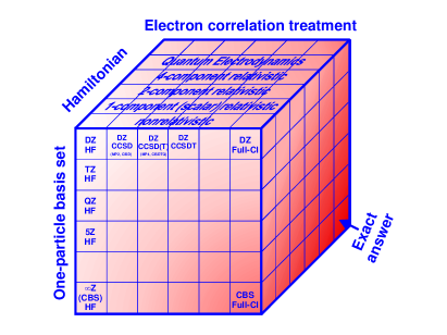
Figure 1: The three axes of the computational cube of wavefunction-based electronic structure theory represents three important approximations. The figure was first published in Tarczay et al. (2001).

For all systems of chemical interest, the exact solution to the (nonrelativistic, time-independent) electronic Schrödinger equation cannot be obtained; thus, a hierarchy of increasingly accurate wave function approximation methods is needed beyond the BO separation of nuclear and electronic motions Császár et al. (2000). Basic to the understanding of this hierarchy and of the uncertainty at any given level is the computational cube depicted in figure 1. It demonstrates that there are three fundamental approximations in polyatomic electronic structure theory:

• choice of the electronic Hamiltonian;

• truncation of the one-particle basis (often referred to as the atomic orbitals);

• the extent of the electron correlation treatment, the $n$-particle basis.

The target result corresponding to the three simultaneous limits is approached as closely as possible by choosing an appropriate Hamiltonian and extending both the one-particle basis set and the many-electron correlation method ($n$-particle basis) to technical limits. For lighter elements, perhaps up to Ar(Z=18), the effects of special relativity will not be consequential (see the previous section), except in electronic structure studies seeking ultimate accuracy.

The ab initio limit can be approached by composite schemes that employ multiple electronic structure computations at different levels of theory to arrive at a single energy for a given molecular geometry. A general composite scheme that is highly successful is the FPA approach Császár et al. (1998). A fundamental characteristic of this approach is the dual extrapolation to the one- and $n$-particle limits of electronic structure theory. The process leading to these limits can be characterized as follows:

• use of a family of basis sets, such as (aug)-cc-pV$X$Z Dunning (1989), which systematically approaches completeness through an increase in the cardinal number $X$, as a key aspect of FPA is the assumption that the higher order correlation increments show diminishing basis set dependence;

• application of lower levels of theory (typically, HF and MP2 computations) with very extensive basis sets;

• execution of a sequence of higher order correlation treatments with the largest possible basis sets;

• layout of a two-dimensional extrapolation grid based on the assumed additivity of correlation increments, that is, the differences between correlation energies given by successive levels of theory in the adopted hierarchy.

Within the FPA approach one considers the consequences of several “small” physical effects:

• core electron correlation;

• special relativity;

• adiabatic and nonadiabatic corrections to the BO approximation;

• quantum electrodynamics (QED).

In diatomic molecules containing first-row atoms several effects due to core correlation have been established Császár and Allen (1996). Equilibrium bond lengths experience a contraction of about 0.001 Å for single bonds and 0.002 Å or more for multiple bonds. The direct effect of core correlation is a correction function to the valence diatomic potential energy curve that has negative curvature at all bond lengths around the equilibrium position. Core correlation decreases all higher order force constants.

For extremely accurate structural studies the corrections to the BO approximation cannot be neglected, especially if light atoms are present in the system.

QED also provides electronic radiative corrections (or Lamb shifts) arising from the interaction of the electron with the fluctuation of the electromagnetic field in vacuum. Studies of atoms, see above, and simple molecules Pyykkö et al. (2001) have indicated that QED effects are generally orders of magnitude smaller than scalar relativistic corrections.

Molecular properties are also an important result of electronic structure calculations, not least because they provide input into subsequent scattering calculations. FPA-type approaches are now being used to provide uncertainty estimates for permanent dipole moments Lodi et al. (2008, 2011). There are two viable methods of calculating dipole moments associated with a given electronic wave function. The most straightforward method, implemented directly in standard quantum chemistry codes, is to compute the dipole moment as an expectation value (EV). An alternative method is to compute the dipole moment studying the response to the application of a (small) electric field placed in appropriate directions by finite differences (FD) of the perturbed energies. The methods are related by the Hellmann-Feynman theorem Jensen (2006), but in general this theorem only holds when exact wave functions are used. In practice, differences between the two methods can be large Lipiński (2002). EV dipoles are cheaper to compute, indeed they are essentially free once a wave function is available, whereas FD dipoles require the computation of extra points with a finite field. However, minor contributions to the dipoles, e.g., non-BO or relativistic effects, can be evaluated in the FD approach using energy differences even when their contribution to the electronic wave function is unknown. Furthermore, there is a general acceptance Werner et al. (1983); Ernzerhof et al. (1992); Lodi and Tennyson (2010) that the FD approach converges more quickly to the true answer for a given (approximate) wave function. We therefore recommend the adoption of this approach to the uncertainty assessment for dipole moments. We note that, unlike the situation with the use of different gauges for photoionization calculations Pindzola and Kelly (1975); Griffin et al. (2009), thus far comparison of EV and FD approaches have provided little insight into the uncertainty in a given calculation.

Even less effort has been dedicated to the computation of transition dipole moments, despite their importance for electronic spectra and as inputs to scattering calculations. However, FD methods for evaluating transition dipoles are available Adamson et al. (1998) if not extensively used. Studies Lodi et al. (2015); McKemmish et al. (2016) suggest that while the FD approach for transition dipoles shows improved convergence behavior compared to the EV approach, perhaps more so than for the diagonal dipole moments, there are technical issues with their use that still need to be overcome McKemmish et al. (2016); Tennyson et al. (2016).

Target polarization is an important property for scattering calculations. However, the target polarizability rarely enters directly into the scattering model. Even when it does, it usually enters only in the long range part of the potential Jain and Gianturco (1991). How well a given scattering model represents the target polarizability can be used as a proxy for how converged the polarization potential is as a whole. If the model gives a poor representation of the target polarizability, then the representation of the overall polarization effect is likely to be poor. The components of the dipole polarizability tensor can be computed using the formula

$$\alpha_{rs}=2\sum_{n>0}\frac{<0|\mu_{r}|n\!><n|\mu_{s}|0\!>}{E_{n}-E_{0}},$$ (1)

where the $\mu$ are dipole operators, and $r$ and $s$ represent Cartesian components. Here $E_{n}$ and $|n\!>$ represent the electronic energy and associated electronic wave function for the $n$-th electronic state of the system; the state for which the polarizability is being calculated is labeled $|0\!>$, but it does not have to be the ground state. For the ground state this series converges from below, provided enough states are included in the expansion. Experience Jones and Tennyson (2010); Brigg et al. (2014) shows that (a) convergence to the correct value requires consideration of the continuum; and (b) sums running over only bound states show apparent convergence to a value that is too low. These issues are illustrated in figure 2.

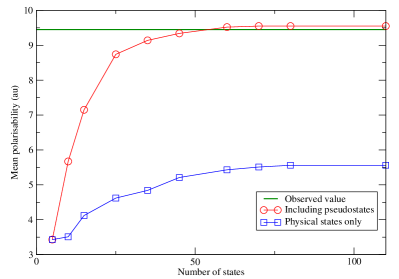
Figure 2: Spherically averaged polarizability of water in its equilibrium geometry computed using sum-over-states formula (1) Jones and Tennyson (2010); the experimental value is corrected for vibrational effects Jonsson et al. (1997).

Use of Eq. (1) can therefore demonstrate the adequacy of a chosen close-coupling expansion. However, when doing this one also should note that approximate wave functions, such as those given by the HF approximation, are usually more polarizable than accurate wave functions. A cancellation of errors can therefore arise, whereby an inaccurate target representation is combined with an incomplete sum over states yielding a polarizability in apparent agreement with experiment or better computations.

III.3 Molecular electronic excited state properties

Excited electronic states are of interest in their own right and form an important component of scattering calculations, where their representation is important both for electronic excitation studies and as part of close-coupling expansions. There are far fewer systematic studies of the convergence of excited state calculations with respect to the various components discussed above. FPA has been used for the study of properties of excited electronic states only to a limited extent DeYonker et al. (2014); Valeev et al. (2001); Bokareva et al. (2009). Indeed an issue for many scattering studies, both theoretical and experimental, is that generally there are far fewer studies of excited states of different spin symmetry than the ground state, since excitation of such states is optically forbidden. However, the lowest excited state is usually in this class.

Molecular excited electronic states can be classified as valence, roughly corresponding to rearrangement of the electrons within the valence orbitals, and Rydberg, corresponding to a loosely bound electron orbiting a parent ion. Different techniques are required to give good representations of these two types of states Little and Tennyson (2013), even though many molecular states are either a mixture of the two or change their character as a function of bond length. We note that Rydberg states form regular series, which are often well represented by quantum defect theory Jungen (1996). Experience shows that uncertainties in these states can also often be better represented in terms of quantum defects rather than absolute energies Tennyson (1996); Schneider et al. (2000), although other methods can be used for calculations including assessment of uncertainties Cocks et al. (2010).

IV Uncertainty Estimates for Electron Scattering Calculations

Before going into uncertainty assessment for collision processes, it is advisable to recognize that there are a number of energy ranges for which particular methods have been developed and are believed to be particularly suitable. The confidence in a given method is usually based on general scattering theory, some numerical examples, and – last but not least – comparison with experimental benchmark results. There is, however, never a guarantee in collision physics, although some variational principles exist (e.g., for the eigenphase sum).

In general, the energy ranges of interest are:

• low energy collisions, with incident projectile energies well below the first electronic inelastic threshold;

• low energy, near-threshold collisions, with projectile energies well below the first ionization threshold;

• intermediate energy collisions, with incident projectile energies from about the first ionization threshold to a few times that value;

• high energy collisions, with projectile energies exceeding several times the first ionization threshold;

• collisions with relativistic energies, in which the kinetic energy of the incident projectile should no longer be described by the nonrelativistic formula.

There is a wealth of literature available on methods for electron scattering calculations; hence we refer to recent reviews Bartschat (2013); Bartschat and Zatsarinny (2015); Burke (2011); Tennyson (2010). However, we emphasize again that there is no unambiguous rule regarding the reliability of a particular method. As will be further discussed below, there are simply too many parameters other than the collision energy that may come into play. Nevertheless, it seems useful to provide some general guidelines based on this one parameter.

For low energy collisions a one-state close-coupling expansion may provide a good start. In contrast to potential scattering (which is a further simplification if the potential is chosen as local, i.e. only depending on the position of the scattering projectile), the approach can properly contain exchange effects. On the other hand, even the closed channels can have a major influence by polarizing the target. This effect is often accounted for by some real-valued “optical” potential (local or nonlocal). In fact, the method can be pushed toward higher energies by including an imaginary “absorption” potential to account for loss of flux into inelastic channels.

Moving on to the near-threshold regime, the close-coupling expansion containing a number of $n$ discrete states (to be referred to as “CCn” below) has been the method of choice for many years. It is often highly successful in the description of resonances associated with low-lying inelastic thresholds. However, the method may have problems in the low energy regime if significant polarization effects originate from coupling to higher-lying discrete states and, in particular, the ionization continuum.

For intermediate energy collisions, the above-mentioned effect of coupling to discrete states omitted in the CCn expansion, and even more importantly to the ionization continuum, should be accounted for in some way. One way to do this is to extend the CC expansion by including a number of so-called “pseudo-states”, which are essentially finite-range states that are forced to fit into a box. For the general idea, details of the box are not important; it only matters that the states are square-integrable and provide a way to discretize the (countable) infinite Rydberg and the continuous ionization spectra. This is the basic idea behind the “convergent close-coupling” (CCC) Bray et al. (2012) and “R-matrix with Pseudo-States” (RMPS) Bartschat et al. (1996); Gorfinkiel and Tennyson (2004) approaches. While the implementations may vary greatly, the critical idea is exactly the same in both methods. Hence, if the same states (physical and pseudo) are included in the expansion, the final results should be the same – except for numerical issues that may remain in practice.

Other ways to account for the possibility that two electrons may leave the target after the collision (but only one of the electron wave function fulfills the correct boundary conditions in the CC approach) include “time-dependent close-coupling” (TDCC) Colgan et al. (2002) and “exterior complex scaling” (ECS) Rescigno et al. (1999). In the former, a wavepacket is used for the projectile and the formalism is expressed as an initial value rather than a boundary value problem. In the latter, the coordinate system is changed from a real to a complex radial grid in order to transform the oscillatory character of the positive-energy continuum wave function to an exponentially decreasing character that, once again, allows for proper evaluation of certain integrals. CCC, RMPS, TDCC, and ECS have been highly successful in handling ionization processes in particular, although the extraction of the relevant information is by no means trivial. For details we refer to some of the references given, which however should only be considered as a starting point. Regarding actual applications to date, ECS has not really been used for production calculations of atomic data relevant for plasma modeling, TDCC has been used mostly to check other approaches for quasi-one and quasi-two electron targets, CCC has been applied over a wide range of the latter targets, while RMPS has been applied also to targets with more complex structure, in particular the noble gases beyond helium as well as other open-shell systems.

Moving on to the high energy regime, perturbative methods based on some form of the Born series are generally the method of choice. In this case, the projectile is either described by a plane or a distorted wave, and then the transition matrix elements are obtained by relatively straightforward integrations. The first-order Distorted-Wave Born Approximation (DWBA) Taylor (1972); Joachain (1984); Madison and Shelton (1973); Itikawa (1986) has the advantage over the corresponding plane-wave (PWBA) version Bote and Salvat (2008) in that it accounts for some higher order terms of the plane-wave series. In practice, production calculations of atomic data in the high energy regime are mostly being performed in the DWBA approach Gao et al. (2006); Al-Hagan et al. (2009); Toth and Nagy (2011); Zhang et al. (2014). If possible, a good check of the applicability of the method involves pushing it toward the intermediate energy regime and then comparing the predictions to those from more sophisticated methods. The present implementation of the CCC approach in momentum space is particularly useful in this respect, since the limiting case of the CCC T-matrix elements for high energies is actually the DWBA or PWBA result.

Regarding the high energy range, full-relativistic implementations of RMPS Badnell (2008), CCC Fursa and Bray (2008), and DWBA Zuo et al. (1991) exist and are frequently used, especially for heavy targets and when the description of explicitly spin-dependent effects (beyond exchange) is desirable. This may, indeed, be necessary since (in a classical picture) the kinetic energy of the projectile may be relativistic near the nucleus even if it is nonrelativistic in the asymptotic regime far away from the target. In this paper we will not consider collisions for which the initial energy is already relativistic.

Finally, we mention the existence of semi-empirical methods, such as the “Binary Encounter f-scaling” (BEf) Kim (2001) and “Binary Encounter Bethe” (BEB) Kim and Rudd (1994) approaches to electron impact excitation and ionization. While these methods are highly useful in practice, they are somewhat limited in scope. For example, BEf can only be used for optically allowed transitions and also requires experimental or reliable theoretical data for rescaling. We do not feel comfortable to suggest a method for an uncertainty assessment for these approaches.

As mentioned above, there are many issues that contribute to the problem of uncertainty assessment in scattering calculations. These include:

• Target properties (energy levels, polarizability, dipole and higher moments), which are ultimately associated with the quality of the wave functions used.

• Model contributions, including:

  • The need for a consistent treatment of the $N$-electron target vs. the $(N+1)$-electron collision problem, which is a critical issue in obtaining accurate resonance positions;

  • accounting for the nuclear motion in electron-molecule collisions.

• Numerical uncertainty.

Some of these issues will be elaborated further below. Not surprisingly, the major challenge is to propagate the uncertainty associated with the above lists to give a final uncertainty on the quantities of interest (see below). We suggest that:

• Calculations be performed for a range of target models, thereby reflecting the underlying uncertainty in the target properties.

• Attempts be made to quantify uncertainties associated with the choice of the scattering model; this will need to be done on a case-by-case basis (see below).

• Numerical uncertainties be quantified similarly to the FPA procedure described above.

IV.1 Electron – atom/ion scattering

There is a wealth of experimental observables in the field of electron collisions with atoms, ions, and molecules. For a fixed incident projectile energy and direction (even those could, of course, be represented by some distributions), the most general (and hence least specific) observable is the grand total cross section, obtained by integrating over all processes, energies, angles, angular momenta, spins, their components, etc.. Such a cross section is certainly relevant and can sometimes (but not always) be measured with high accuracy in transmission cells or via the loss of the target species in traps. The grand total cross section is made up of sums or integrals over unobserved quantities, where the lack of observation is not a requirement of quantum mechanics, but rather a choice of the experimenter. This choice may be voluntary or involuntary. In the former case, one might only be interested in a rather global set of parameters to model a system, while the latter case might be forced if the signal rate is simply inadequate to measure what one would really like to know.

It is clearly unrealistic to discuss all possible cases, including also those not even specified above, where the initial projectile and target beams might have been prepared beyond an unpolarized ensemble. We therefore restrict our discussion to angle-integrated state-to-state cross sections and in some cases the rate coefficients that can be derived from them by performing an integral over the incident projectile energy.

For electron collisions with atoms and ions, the processes of interest for the present paper, including initially excited states, are:

• elastic + momentum transfer;

• inelastic (excitation);

• inelastic (ionization);

• dielectronic recombination.

A few illustrative examples about how one might attempt to quantify uncertainties in theoretical predictions for these processes will be given in section VI.

IV.2 Electron – molecule scattering

Many of the issues involved in uncertainties for electron-molecule scattering are similar to those for atoms so below we concentrate on those that differ.

Processes of interest, including those starting from initially excited states, are

• elastic and momentum transfer collisions;

• inelastic, rotational excitation;

• inelastic, vibrational excitation;

• dissociative electron attachment or recombination;

• inelastic, electronic excitation;

• impact dissociation, which normally goes via electronic excitation;

• ionization.

These processes (listed in approximate order of increasing collision energy) involve a mixture of electronic excitation (either directly or via impact dissociation or ionization) and excitation of the (rotational or vibrational) nuclear motion. There is no current, general method that solves for all these processes simultaneously in a unified self-consistent manner. For example, most treatments of electronic excitation or ionization are performed at the fixed nuclei level whereas treatments of dissociative attachment or recombination use specially adapted nuclear motion techniques employing resonance (potential energy) curves which are computed in electron collision calculations. See refs. Laporta et al. (2012, 2015) for example.

In practice nuclear motion is often introduced in a somewhat ad hoc fashion deemed appropriate for the process of interest. For example, resonances greatly enhance vibrational excitation cross sections and these can be computed in a relatively straightforward fashion using resonance curves, see ref. Laporta et al. (2015). Conversely, nonresonant vibrational excitation can be treated by vibrationally averaging T-matrices as a function of geometry Chang and Fano (1972); Morrison et al. (1984).

The vibrational averaging of the geometry-fixed scattering (or T-) matrices is a part of the frame transformation approach Chang and Fano (1972); Atabek et al. (1974); Greene and Ch.Jungen (1985), developed in the 1970s and 1980s to account for non-BO couplings of the incident electron with the vibrational and rotational motion of the target molecule. For collisions with molecular ions, the frame transformation can be combined with multi-channel quantum defect theory (MQDT) Seaton (1966); Aymar et al. (1996) to give an approach that unifies nonresonant and resonant processes in electron-molecule scattering Atabek et al. (1974); Greene et al. (1979); Greene and Ch.Jungen (1985); Gao and Greene (1989, 1990) including rovibrational and electronic resonances, and that accounts for non-BO couplings and vibrational excitation of the target by the incident electron. Full vibrational close-coupling also provides a means of treating resonant and nonresonant processes simultaneously for electron collisions with neutral molecules, but it is rarely used Sun et al. (1995).

Rotational motion and excitation of the target molecule are often treated by means of a transformation from the body-fixed frame to the laboratory frame by simple angular momentum recoupling Chase (1956), which can be viewed as a part of the general frame transformation approach discussed above Faure et al. (2009a, b); Kokoouline et al. (2010). If one uses the rigid-rotor approximation, the purely rotational frame transformation is analytical for linear, spherical, or symmetric top molecules and, therefore, is easy to implement Faure et al. (2009a, b). The rotational frame transformation approach has been demonstrated to work very well when compared to full close-coupling treatments Faure et al. (2009a). For molecules with permanent dipole moments, however, rotational excitation requires special treatment because the long-range interaction of the electron with the target dipole moment means that a large number of partial waves should be taken into account. Special hybrid treatments are used to provide the contribution of the higher partial waves Norcross and Padial (1982); Sanna and Gianturco (1998).

Along with rotational and vibrational excitation, dissociative electron attachment and dissociative recombination (DR) are the dominant low energy processes. The cross sections for these dissociative processes are very sensitive to the locations of curve crossings between the dissociative resonance state(s) and the target curve; the resulting cross sections are known to be highly sensitive to this aspect of the calculation O’Malley (1966); Bates (1991); Guberman and Giusti-Suzor (1991); Morgan and Noble (1984); Schneider et al. (2000).

There is a hierarchy of non-perturbative low-energy electron-molecule collision models. The simplest one currently in use is the static exchange (SE) model, which considers electron collisions with a target represented by a Hartree-Fock wavefunction. In the SE model the electron is allowed to occupy empty (“virtual”) target orbitals but the target itself remains frozen. The SE model is well-defined, which makes it useful for cross-comparison of codes but limited in the amount of physics included. For example SE calculations can give low-lying shape resonances but usually they are too high in energy and too broad; Feshbach resonances, which involve simultaneous target excitation and trapping of the scattering electron, cannot be represented in this model. Inclusion of polarization effects using the static exchange plus polarization (SEP) model is often found to give reliable parameters for low-lying shape resonances; converging SEP calculations usually requires the inclusion of many more virtual orbitals than are required to converge the simple SE model for the same system Fujimoto et al. (2012). Conversely Feshbach resonances, which dominate the DR process, are best represented by models that contain their parent state as part of a close-coupling expansion.

For collisions with a molecular ion having a closed electronic shell, the energy surface of the neutral dissociative potential usually crosses the ionic surface far from the geometry of the equilibrium of the target ion. In this case, the actual geometry at which the ionic and dissociative potential surfaces cross is irrelevant, because the DR cross section is determined by the probability of electron capture into a state different than the dissociative state. During such a process the target ionic core is excited rovibrationally and the electron is captured into a weakly-bound Rydberg state. This is the so-called indirect DR mechanism Bardsley (1967); Bates (1991), which is dominant for many closed-shell molecular ions Kokoouline et al. (2011); Douguet et al. (2012a, b); Fonseca dos Santos et al. (2014). The accuracy of the theoretical DR cross section in the indirect process, via intermediate molecular Rydberg states and rovibronic resonances, is mainly determined by the accuracy of representing the non-BO coupling responsible for the incident electron capture. Expressed in terms of the electron-molecule scattering matrix $S_{i^{\prime}v^{\prime};iv}$ the DR cross section is $\sigma\sim|S_{i^{\prime}v^{\prime};iv}|^{2}/E$, where indices $v^{\prime}$ and $v$ represent final and initial vibrational states of the ion during the capturing process, and $i^{\prime}$ and $i$ describe electronic states. The matrix element $S_{i^{\prime}v^{\prime};iv}$ is obtained by integrating the geometry-fixed scattering matrix over vibrational states $v^{\prime}$ and $v$. For small molecules, the numerical accuracy of vibrational wave functions is usually relatively good, and the uncertainty of the final cross section is mainly determined by the quality of the geometry-fixed scattering matrix. For larger polyatomic ions, the inaccuracy of wave functions, which are usually calculated using the normal-mode approximation Kokoouline et al. (2011); Douguet et al. (2012a, b); Fonseca dos Santos et al. (2014), may contribute significantly to the uncertainty of the final DR cross section. Therefore, assuming that the accuracy of the vibrational wave functions is good, the uncertainty of the final DR cross section for the indirect mechanism (for most closed-shell molecular ions) is $\Delta\sigma/\sigma\sim 2|\Delta S|/|S|$, where $S$ and $\Delta S$ are the geometry-fixed scattering matrix and its uncertainty. The scattering matrix for DR calculations can be computed using electron scattering codes, such as R-matrix, complex Kohn, or variational Schwinger methods. Recent examples, include Fonseca dos Santos et al. Fonseca dos Santos et al. (2014) who obtained their geometry-fixed scattering matrix using the complex Kohn calculations, and Little et al. Little et al. (2014) who performed similar calculations based on R-matrix computations. Comparisons have shown that these two methodologies yield very similar results for a given scattering model Faure and Tennyson (2002). A second method, used extensively in earlier studies Kokoouline and Greene (2003a, b); Kokoouline et al. (2011); Douguet et al. (2012a, b), is based on quantum defects extracted from energies of Rydberg states of the corresponding neutral molecule. The Rydberg-state energies are usually obtained ab initio, but experimental energies have also been used Jungen and Pratt (2008a, b, 2009).

At collision energies near threshold electronic excitation provides an important new channel. For this situation CCn-type models are usually employed. Such calculations face all the difficulties described above for atoms plus complications introduced by loss of symmetry and nuclear motion encountered in molecules.

The intermediate energy region is beginning to be explored with fully ab initio methods but only for rather simple systems Gorfinkiel and Tennyson (2005); Halmová and Tennyson (2008); Pindzola et al. (2012); Colgan and Pindzola (2012). Conversely, extensive studies for the high energy region were performed using various perturbative approximations such as the Born or DWBA approximations Gao et al. (2005, 2006); Kaiser et al. (2007).

V Uncertainty Assessment for Charge Transfer Collisions

When the incident electron in a collision with an atomic or a molecular target is replaced by a positively charged ion a new channel appears: electron transfer. Since this channel is the most important one for plasma and related applications we will concentrate on such charge transfer collisions in this section.

It goes without saying that an accurate solution of the full Schrödinger equation is not feasible, except maybe for the simplest charge transfer collision systems involving just two nuclei and one electron. Accordingly, and similarly to what has been discussed for electron scattering in section IV, different approximation methods have been developed, which are deemed suitable in different energy ranges.

The situations of interest for charge transfer collisions are:

• very low energy collisions, in which the de Broglie wavelength associated with the projectile motion is comparable with the length scale that is characteristic for electronic processes;

• low energy collisions, in which the projectile de Broglie wavelength is too small to resolve electronic processes, but the projectile-target interaction time is still long compared to the characteristic electronic time scale;

• intermediate energy collisions, in which the relative projectile-target speed is comparable with the orbital speeds of the active electrons;

• nonrelativistic high energy collisions, in which the previous condition is no longer fulfilled;

• relativistic energy collisions.

Note that we are using a similar nomenclature as in section IV, although the actual magnitudes of the collision energies are very different for electron vs. heavy particle projectiles.

An authoritative overview of the entire spectrum of theoretical charge transfer methods available by the early 1990s was given by Bransden and McDowell Bransden and McDowell (1992). For more recent, but somewhat more specialized accounts we refer the reader to Belkić (2008); Loreau et al. (2014) and references therein. The following paragraphs are meant to provide a (necessarily incomplete) mini-survey of what is discussed in those works and what else is of relevance in the context of this article.

The gold standard for the calculation of charge transfer cross sections from very low up to intermediate projectile energies has long been one or another variant of the CC expansion. Accordingly, limitations in basis-set convergence are the main source of numerical uncertainties. Most of these CC calculations are also afflicted by model uncertainties, because it is normally not the full Schrödinger equation that is cast into matrix-vector form.

One gets closest to the ideal of a calculation free of model uncertainty in the very low energy regime in which a fully quantum mechanical description of the scattering system is required. In this region, electron transfer usually dominates the dynamics and can be understood by considering the real and avoided crossings of a small number of potential energy curves of the quasimolecular system of projectile and target. Accordingly, an expansion in terms of products of molecular electronic states and nuclear wave functions is the standard method of attack. In its original form this so-called perturbed stationary state (PSS) approach has inherent defects, because individual terms in the expansion do not satisfy the boundary conditions of the scattering problem, thereby introducing spurious origin-dependent couplings in a finite matrix representation of the Schrödinger equation Delos (1981). These defects can be remedied by including electron translation factors (ETFs) or by using reaction coordinate techniques Delos (1981); Errea et al. (1994). An alternative method is the hyperspherical close coupling (HSCC) approach, in which a rescaled Schrödinger equation written in terms of hyperspherical coordinates is solved (see ref. Liu et al. (2005) and references therein).

In modern applications to few-electron systems the molecular states and couplings are calculated with sophisticated quantum chemistry methods, which implies that electron correlations are taken into account and the general approach can be called ab initio Zygelman et al. (1997). It has become customary, albeit somewhat inaccurate, to refer to these modern versions of the PSS approach as quantum mechanical molecular-orbital close-coupling (QMOCC) calculations Li et al. (2015), and we follow this convention.

Moving up in collision energy to, say, 1 keV/amu and higher, fully quantum mechanical methods become challenging because they normally involve partial-wave or other expansions of the scattering amplitude that become very large in the low energy region. Very recently, the three-body problem of proton-hydrogen scattering has been addressed in a fully quantum mechanical CCC approach that solves the Lippmann-Schwinger integral equations for the scattering amplitudes Abdurakhmanov et al. (2016). The more traditional approach is to make use of the smallness of the projectile de Broglie wavelength by adopting a semiclassical approximation. As long as one is interested in total (i.e.  integrated over projectile scattering angle) cross sections only, the semiclassical approximation amounts to reducing the full scattering problem to a time-dependent Schrödinger equation (TDSE) for the electronic motion in the field of classically moving nuclei. The classical trajectories can be determined by considering the nonadiabatic coupling of the electronic and the nuclear motion as is done in the electron nuclear dynamics (END) method Deumens et al. (1994); Cabrera-Trujillo (2010), or by using Coulomb or model scattering potentials Green et al. (1982a, b); Fritsch and Lin (1984); van Hemert et al. (1985). At collision energies of a few keV/amu and higher, simple straight-line trajectories are just as good, i.e. the numerical error introduced by replacing a curved trajectory by a rectilinear one is negligibly small compared to errors associated with basis-set convergence issues or other numerical uncertainties. The same can be said about the semiclassical approximation itself: at least for total cross section calculations it is essentially exact in and above the low energy regime.

In the low energy regime electron transfer still is the strongest electronic process and molecular state expansions (including ETFs) still are the most widely used methods Fritsch and Lin (1991). Within the semiclassical framework they are often referred to as MOCC methods (without the ’Q’).

Once direct target ionization, i.e. transitions into the continuum, become important other CC techniques or fully numerical methods for the solution of the semiclassical TDSE gain importance. A common feature of the former is that, similar to what has been discussed for electron scattering, positive energy pseudo-states are included to discretize the continuum. Even if one is not interested in direct target ionization one cannot simply close the ionization channel in a calculation without running the risk of degrading the results for target excitation and electron transfer. It is characteristic of the intermediate energy regime that all channels are coupled and have to be taken into account simultaneously. Examples of suitable intermediate energy CC methods are the two-center atomic-orbital, AOCC, method Fritsch and Lin (1991) and the two-center basis generator method (TC-BGM) Zapukhlyak et al. (2005), both of which include bound (atomic) target and bound (atomic) projectile states, endowed with ETFs, and sets of pseudo-states whose explicit forms vary.

Notwithstanding considerable success in applications to charge transfer collisions these methods can be criticized for being built on formally overcomplete basis sets. Indeed, there are known cases in which too large basis sets on both centers (perhaps combined with insufficient numerical accuracy in the calculation of matrix elements) have led to spurious couplings and unphysical results Kuang and Lin (1997), meaning that the bigger (the basis), the better (the convergence) is not necessarily true for these two-center methods. The insight that completeness of a basis is not necessary, in principle, for following the evolution of the time-dependent state vector exactly Kroneisen et al. (1999) does not help in practice, since there is no other practical criterion available than checking for changes in the results when more basis states are added. One-center expansions are not afflicted by the overcompleteness problem, but are in practice inferior to two-center methods when it comes to separating electron transfer from ionization to the continuum.

As indicated above, direct numerical approaches to the solution of the semiclassical TDSE offer an interesting alternative to CC expansions. The basic idea is straightforward: represent the electron wave function on a grid (usually in coordinate space) and propagate it in time by application of the time-evolution operator over a large number of small time steps. This can be done in different ways, e.g., by using the split-operator Fast Fourier transform method. Whichever technique is used, most time-dependent lattice (TDL) methods share the following features: (i) the Coulomb potentials of the nuclei are replaced by soft-core potentials; (ii) absorbers are introduced to avoid unphysical reflections of the wave function at the boundaries of the numerical box; (iii) numerical accuracy mostly depends on the spatial grid parameters (provided a sufficiently small time step size is used for the propagation). One attractive feature of TDL approaches is that they provide a view on the electron density distribution in the continuum, i.e. insight into electron emission characteristics, but they have also been applied successfully to charge transfer problems Minami et al. (2006); Pindzola and Fogle (2015).

As in the case of electron scattering, perturbative methods and distorted-wave approaches are the principal methods of choice in the nonrelativistic high energy regime. They can be formulated on the level of the semiclassical approximation or for the full quantum mechanical problem, and at least for some of the methods put forward over the years both options can be shown to be (essentially) equivalent Bransden and McDowell (1992). Numerical uncertainties are usually well controlled, at least in first-order models, but model uncertainties can only be estimated by extensive comparisons with other (preferably nonperturbative) calculations and with experimental data.

Most of the approaches discussed in this section have been generalized to deal with collisions at relativistic energy. The principal motivation for studying this regime is the fundamental interest in relativistic dynamics and phenomena such as radiative charge transfer and electron-positron pair production. While the former process can also be of importance at very low collision energies Bransden and McDowell (1992); Li et al. (2015), the latter is, of course, a truly relativistic effect. Since relativistic collisions are less relevant for applications, we will not discuss them further in this article.

We end this brief survey of charge transfer methods with a few general comments. First, the majority of methods touched upon in this section deal with true or effective one-electron problems. The two-electron problem has been addressed in a number of perturbative models Belkić et al. (2008), and also in the framework of the semiclassical CC approach Fritsch and Lin (1991). As mentioned above, modern (Q)MOCC methods can deal with many-electron systems in an ab initio fashion, but they have mostly been applied to one-electron transitions, i.e. single electron transfer Li et al. (2015); Zygelman et al. (1997). For truly many-electron problems, such as multiple electron transfer to a highly charged ion, simplifications are unavoidable, which implies that further modeling, usually on the level of the semiclassical TDSE, is necessary. An obvious idea is to replace the many-electron Hamiltonian by a sum of effective one-electron Hamiltonians, i.e. to solve the problem on the level of the independent electron model (IEM). This has worked quite well in several instances, but it is not obvious how to carry out a reliable uncertainty assessment of an IEM calculation. One way to go about this is to consider several variants of IEM calculations, e.g., by varying the effective potentials used within reasonable bounds, and monitor the spread of results obtained. It will be illustrated in section VI.4 that this is a useful procedure, although it can give at most qualitative information on the uncertainty of a given IEM calculation.

Second, echoing a comment made in section IV for electron scattering, we mention that simpler, sometimes semi-empirical and/or classical methods for calculating charge transfer cross sections have been widely used over many years. Among them are two-state quantum mechanical models (see ref. Bransden and McDowell (1992)), variants of the classical over-barrier model Niehaus (1986), and the classical trajectory Monte Carlo method Olson and Salop (1977). The latter in particular has been highly successful in many applications, even in the low energy regime Otranto et al. (2014) in which quantum effects are deemed important. An implication of this somewhat surprising observation is that uncertainty estimates have to rely on extensive comparisons with more rigorous quantum mechanical methods and with experimental data.

Third, in many cases the observables of interest are not electron transfer cross sections, but cross sections associated with post-collisional events such as radiative de-excitation of excited projectile states or the fragmentation of the target in ion-molecule collisions. This requires further modeling, and hence it introduces further uncertainties and also the problem of uncertainty propagation. Again, it seems that the only known and practical way of dealing with these issues is to perform computations for a range of models and monitor the spread of results. An example for this will be given in section VI.4.

VI Illustrations

VI.1 Structure

The best examples of uncertainty estimates in high-precision theory are provided by few-electron atoms. Hydrogen is a special case because there the Schrödinger (or Dirac) equation can be solved exactly, and so the uncertainty comes entirely from higher-order QED terms or nuclear structure effects not included in the calculation (see section III.1). For the two- and three-electron cases of helium-like and lithium-like atoms complete calculations in Hylleraas coordinates have been performed. Recent high-precision measurements Sánchez et al. (2006); Sanchez et al. (2009) and theory Yan et al. (2008b, 2009); Puchalski et al. (2010) for the $1s^{2}2s\;^{2}S-1s^{2}3s\;^{2}S$ two-photon transition in lithium provide an excellent example of what can be achieved. Table 1 lists the various contributions to the transition frequency, expressed as a double power series in powers of $\mu/M$ and $\alpha$, where $\mu/M$ is the ratio of the reduced electron mass to the nuclear mass, and $\alpha$ is the fine structure constant (see table caption for numerical values). The sum of the first three entries gives the total nonrelativistic transition energy, including first- and second-order finite nuclear mass corrections of order $\mu/M$ and $(\mu/M)^{2}$. These account for the nonrelativistic part of the isotope shift, but at this level of accuracy, the usual normal and specific isotope shifts of order $\mu/M$ are not sufficient, and therefore the second-order $(\mu/M)^{2}$ term must also be included. The associated uncertainties shown in Table 1 were reliably estimated from the rate of convergence of the calculation with the size of the Hylleraas basis set. Next comes the leading relativistic correction of order $\alpha^{2}$ relative to the nonrelativistic energy from the Breit interaction, and the relativistic recoil term of order $\alpha^{2}\mu/M$. The uncertainties from all these terms can be accurately estimated from the rate of convergence with the size of the Hylleraas basis set. At the next level are the QED corrections of order $\alpha^{3}$, corresponding to the Lamb shift in hydrogen. The theory for these terms is complete in terms of known expectation values of operators, including both the electron-nucleus and electron-electron QED contributions (the Araki-Sucher terms). The dominant source of uncertainty are the Bethe logarithms for the states of lithium Yan and Drake (2003). The terms of order $\alpha^{3}\mu/M$ are radiative recoil corrections due to the finite nuclear mass. These can be calculated to more than sufficient accuracy in terms of known operators Yan and Drake (2003). The dominant source of uncertainty in the theoretical transition frequency comes from the higher-order QED corrections of order $\alpha^{4}$ and $\alpha^{5}$, since the basic theory for these terms has not yet been developed. However, estimates can be obtained from the corresponding QED shifts in hydrogen with appropriate scaling with the nuclear charge and electron screening, as shown in the table, with 10% and 25% uncertainties assigned respectively for these two terms. Finally, the correction due to the finite nuclear charge radius is included.

Table 1: Theoretical contributions to the $1s^{2}2s\;^{2}S-1s^{2}3s\;^{2}S$ transition energy (cm^-1) of ⁷Li Yan et al. (2008b, 2009); Puchalski et al. (2010), and comparison with experiment Sánchez et al. (2006). The entries on the left indicate the powers of $\mu/M$ and $\alpha$ that give rise to each contribution relative to the nonrelativistic energy for infinite nuclear mass, where $\mu/M=7.820\,202\,988(6)\times 10^{-5}$ is the ratio of the reduced electron mass to the nuclear mass for an atomic mass of 7.016 003 4256(45) u, and $\alpha=1/137.035\,999\,139(31)$ is the fine structure constant. The contributions of order $\alpha^{4}$ and $\alpha^{5}$ are estimates. Nucl. size is the finite nuclear-size correction for an assumed nuclear charge radius of 2.390(30) fm.

Contribution	Transition Energy (cm-1)
Infinite mass	27 206	.492 847 9(5)
$\mu/M$	–2	.295 854 362(2)
$(\mu/M)^{2}$	0	.000 165 9774
$\alpha^{2}$	2	.089 120(23)
$\alpha^{2}\mu/M$	–0	.000 003 457(9)
$\alpha^{3}$	–0	.187 03(26)
$\alpha^{3}\mu/M$	0	.000 009 74(13)
$\alpha^{4}$ (Est.)	–0	.005 7(6)
$\alpha^{5}$ (Est.)	0	.000 52(13)
Nucl. size	–0	.000 390(10)
Total	27 206	.093 7(6)
Expt. Sánchez et al. (2006)	27 206	.094 082(6)

The final theoretical value 27 206.093 7(6)cm^-1 is in good agreement with the substantially more accurate (2 parts in $10^{10}$) measurement 27 206.094 082(6) cm^-1 (see Table 1.) However, the important lesson to be learned from the comparison is that, since the theoretical uncertainties in the lower order terms are well controlled, the comparison between theory and experiment provides an experimental value for the higher order QED terms of order $\alpha^{4}$ and $\alpha^{5}$ that cannot yet be calculated directly. This same principle has been applied with great effectiveness to determine the nuclear charge radius for a range of halo nuclei from ⁶He to ¹¹Be from the measured isotope shifts Nörtershäuser et al. (2011); Lu et al. (2013). Here, the otherwise dominant uncertainties from the mass-independent QED terms in Table 1 cancel when taking the difference between isotopes with different $\mu/M$, and so the residual difference between experiment and theory with much smaller uncertainties provides an accurate determination of the relative nuclear charge radii.

The pair of articles by Safronova et al. Safronova et al. (2014a, b) describes high accuracy computations with uncertainty estimates for energies of low-lying excited states in Ag-like, Cd-like, In-like and Sn-like ions. The electronic structure for all these states is characterized by a [Kr]$4d^{10}$ core and 1, 2, 3, or 4 valence electrons, respectively. A $5s^{2}$ component in the structure of an In-like or Sn-like ion can optionally be viewed as part of the core, leaving one or two valence electrons. Three models are used in refs. Safronova et al. (2014a, b): the linearized coupled-cluster method including all single, double, as well as partial triple excitations (All-order SDpT), the configuration-interaction plus all-order model (CI+All-order) and the configuration-interaction plus many-body perturbation theory model (CI-MBPT). All three models start from a frozen-core DF potential. The All-order SDpT model is the most computationally intensive, and it is used only for the monovalent systems, i.e. the Ag-like ions and the In-like ions with the $5s^{2}$ electrons included in the core. The CI+All-order and CI-MBPT models are used for monovalent and multivalent systems. Within each model the principal convergence issue arises from the truncation in the partial wave expansion, particularly for the $4f$ shell. Second order perturbation theory is used to evaluate the contribution of partial waves with $l>6$. It is found that this contribution is approximately equal to the contribution from the $l=6$ term, which is then used as an approximation. The Breit term and the QED corrections are evaluated separately. Finally, a 25% uncertainty is assigned to each of the four corrections (i.e.  higher order correlations, higher partial wave contributions, Breit interactions, and QED corrections), and the results are combined via sum of squares to obtain the total uncertainty.

Table 2: Calculations and their uncertainties of the excited state energies of Ce⁹⁺ and Ba⁷⁺ Safronova et al. (2014a). All values are in cm^-1.

Ion	Ce9+		Ba7+
Level	5p3/2	4f5/2	5p3/2	4f5/2
Experiment	33427	54947	23592	137385
All-order SDpT	33406	55419	23564	137770
Diff (Exp – SDpT)	21	–472	28	–385
CI + all	33450	54683	23605	137256
Diff (Exp – CI+all)	–23	264	–13	129
CI+MBPT	33986	54601	24020	137086
High-order correlations	–147	2687	–134	2224
Higher partial waves	14	–1011	12	–858
Breit interaction	–403	–1595	–293	–1197
Uncertainties	130	220

The above considerations yield an uncertainty estimate based strictly on theory. It was applied by Safronova et al. Safronova et al. (2014a) to the In-like Ce⁹⁺, Pr¹⁰⁺, and Nd¹¹⁺ “monovalent” ions where the CI+All-order and the CI-MBPT approach are both applicable. However, Safronova et al. also rely on comparisons with reference ions for which experimental data are available. In ref. Safronova et al. (2014a) the isoelectronic Ba⁷⁺ ion was used as a reference ion. Results from the monovalent All-order (coupled cluster) SDpT model and the CI+All-order model with three valence electrons were compared, and it was found that CI+All-order gave the better agreement with measurement. Table 2 (extracted from Table V of Safronova et al. (2014a)) shows the final computed energies for two levels in In-like Ce⁹⁺ and Ba⁷⁺ together with estimated contributions from high order correlations, higher partial waves, and Breit interaction, and along with uncertainty estimates for the states in Ce⁹⁺. QED corrections were considered to be negligible for this system. The uncertainty estimate for the calculated Ce⁹⁺ energies was obtained as the sum of two contributions: the error (relative to experiment) in the calculation for the Ba⁷⁺ reference ion and the absolute change between the reference ion and the actual ion in the sum of the identified small terms. Finally, these calculated uncertainties were compared with the actual deviation from the experimental energies (which are available for Ce⁹⁺), and it was found that the estimate of uncertainties of calculated energies is reasonable for $4f$ states but significantly larger for $5p$ states.

UQ is being routinely used to determine structural parameters of small molecules within tight uncertainty bounds. This is done, at least in part, to aid the predictions of the rotational spectrum of these species and hence their detection in the laboratory and space Puzzarini et al. (2008); Demaison et al. (2010).

Table 3 illustrates an application of the FPA method to uncertainty assessment of the calculated dissociation energy ($D_{0}$) of H₂¹⁶O. Full details are given by Boyarkine et al. Boyarkin et al. (2013) who provide similar results for water isotopologues. Subsequent measurement of $D_{0}$ for H₂¹⁸O yielded results within the uncertainties of the predicted value Makarov et al. (2015). The uncertainties listed in Table 3 include a contribution of 1 cm^-1 due to nonadiabatic effects, even though these effects were assumed to give a negligible direct contribution to the value of $D_{0}$ and actual calculation of nonadiabatic effects did not form part of the study. An estimate of the magnitude of contributions due to effects neglected in a given model is a part of the uncertainty assessment.

Table 3: Ab initio contributions to the first dissociation energy of H₂¹⁶O. All values are in cm^-1. Uncertainties are given in the last column. Signed contributions are incremental values. Contributions (A) to (H) only concern the electronic motion with fixed nuclei. CBS means complete basis set, FCI is full configuration-interaction, DBOC means the diagonal Born-Oppenheimer correction and ZPE is the vibrational zero-point energy. Contributions (I) to (N) involve solving the nuclear motion problem for water and for the OH diatomic and are therefore nuclear mass dependent (MD). Full details about the components considered in the focal point analysis can be found in Boyarkine et al. Boyarkin et al. (2013).

		Value	Uncertainty
A	CBS CCSD(T) frozen core	43956	6
B	Core correlation CCSD(T)	+81	2
C	All-electron CBS CCSD(T) [=A+B]	44037	6
D	Higher order electron correlation	–52	3
E	CBS FCI [=C+D]	43985	7
F	Scalar relativistic correction	–53	3
G	QED (Lamb shift) correction	+3	1
H	Spin-orbit effect	–69.4	1
I	Angular momenta coupling, OH	+31.5	0
J	Sum spin effects, OH [=H+I]	–37.9	1
K	DBOC, H2O	+35.3	0.5
L	ZPE H2O	4638.1	0
M	ZPE OH	1850.7	0.5
N	Net ZPE, H2O [=L+M]	2787.4	0.5
U	Nonadiabatic contributions	0	1
V	Total MD, H2O [=I+K+N+U]	–2721	1
	$D_{0}$(H2O) Calc. [=E+V]	41145	8
	(Obs – Calc) $D_{0}$(H2O)	+1

One area where uncertainty assessment is beginning to have significant impact is the computation of dipole-moment surfaces Lodi et al. (2008, 2011) and hence rotation-vibration transition intensities Polyansky et al. (2015). The methodology used here is based on adapting the FPA method for computing the dipole moment surface (DMS) and then performing multiple computations using different PESs and DMSs to establish stability of the results Lodi and Tennyson (2012); Zak et al. (2016). These computations are important as it is often difficult to measure absolute transition intensities with the accuracy demanded for the interpretation of modern remote sensing experiments.

VI.2 Electron - atom/ion collisions

As the first example we consider the momentum transfer cross section for low energy electron collisions with Ar atoms; an important parameter for many laboratory plasmas. Figure 3 shows a comparison between experiment and theory. While the agreement with experiment is nearly perfect for the presumably best model (fully relativistic including dynamic distortion (DD) of the target charge distribution by the projectile), the important issue for the present paper is the fact that i) a number of calculations were performed, and ii) that even a nonrelativistic approach with a less sophisticated way of accounting for the above effect yields rather similar results. Because of this, together with the general confidence in the polarized-orbital method as an enhanced one-state close-coupling approach that contains the most important physical effects, one can make reasonable estimates about the position of the minimum (we suggest $\rm 0.15\,eV\pm 0.05\,eV$) and the value of the cross section away from the resonance (10% or better at 0.01 eV and 1.0 eV).

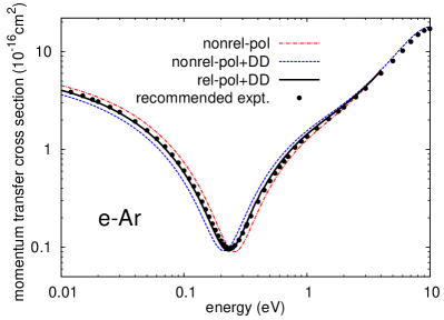
Figure 3: Momentum transfer cross section for electron scattering from argon atoms in their ground state. Results from various polarized orbital calculations (see text) are compared with a recommended set of experimental data Elford (2000) (solid circles). The curve labeled “rel-pol+DD” is a fully relativistic model including dynamic distortion. (Figure taken from Bartschat (2013).)

Figure 4 shows predictions from both CCC and RMPS for electron impact excitation of the $n=2$ states of helium. Once again, it seems possible to make a reasonable estimate of the uncertainty in the theoretical predictions. Even though these computations are nearly 20 years old, they have indeed withstood the test of time. This is ultimately not surprising, since the scattering models contain what we believe is the essential physics, namely an accurate target description (the relevant energy levels and oscillator strengths agree with experiment and much more sophisticated structure-only computations at the 10% or better level) as well as channel coupling within the discrete spectrum as well as to the ionization continuum. Significant differences occur only in the resonance regime near the low-lying excitation thresholds, with the principal reason being that the CCC calculations had only been performed at a few energies. Looking at the comparison, one might conclude that the average of the two sets of theoretical predictions is accurate at least at the 20% level (most likely better). This is something that cannot be said even today for most of the experimental data points, of which there are only very few anyway.

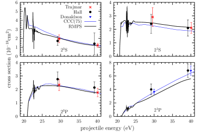
Figure 4: Cross section for electron-impact excitation of the $n=2$ states in helium from the $\rm(1s^{2})^{1}S$ ground state. Three sets of experimental data Trajmar (1973); Hall et al. (1972); Donaldson et al. (1972) are compared with predictions from nonrelativistic CCC Fursa and Bray (1995) and RMPS Bartschat (1998) models. (Figure adapted from Bartschat (1998).)

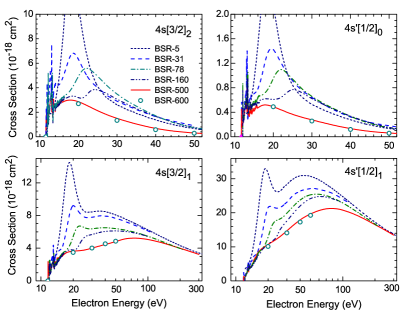
Figure 5: Angle-integrated cross sections for electron impact excitation of the $\rm 3p^{5}4s$ states in argon from the ground state $\rm(3p^{6})^{1}S_{0}$. The results of a number of BSR calculations shows the convergence of the predictions from a close-coupling model. (Figure taken from Zatsarinny et al. (2014)).

Figure 5 is an example of a systematic study regarding the convergence of the close-coupling expansion Zatsarinny et al. (2014). In this particular implementation, the resulting equations are solved using the so-called “B-Spline R-matrix with Pseudo-States” (BSRMPS) approach. Once again, however, we emphasize that it is not the implementation of a particular model that determines the overall uncertainty of its predictions. If the close-coupling expansion could literally be driven to an infinite number of states on an infinitely fine spatial grid, then it should yield the correct solution of the underlying many-particle Schrödinger or Dirac equation. In practice, of course, this is not possible. In the above example, the structure description for the states of interest, the initial $\rm(3p^{6})^{1}S_{0}$ state and the four final $\rm 3p^{5}4s$ states of argon, was carried out as well as the authors believed was necessary for most of the uncertainty to come from the finite size of the close-coupling expansion. This also means that purely numerical errors in solving the equation with a fixed number of states are believed to be negligible.

Looking at the figure, one can see a very strong effect of adding more and more states to the close-coupling expansion. However, going from a 500-state (BSR-500) to a 600-state (BSR-600) model ultimately indicates some convergence. As mentioned several times already, there is no guarantee for the correctness of the final results. Nevertheless, the results change in a systematic way, and it seems as if at the very least the BSR-600 predictions can be taken as a likely upper limit of the “true” solution of the underlying equations, at least outside of the resonance regime.

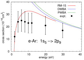
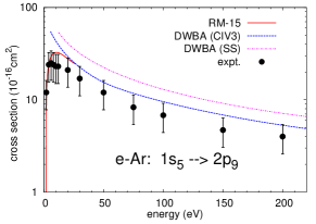
Figure 6: Cross section for electron impact excitation of the $\rm(3p^{5}4s)^{3}P_{2}\to(3p^{5}4p)^{3}D_{3}$ ($\rm 1s_{5}\to 2p_{9}$) (in Paschen notation) transition in argon. A number of theoretical predictions are compared with the experimental data of Boffard et al. Boffard et al. (1999). (Figure taken from Bartschat (2013).)

Moving on to the intermediate energy and high energy regimes, figure 6 shows the angle-integrated cross section for excitation of the $\rm(3p^{5}4p)^{3}D_{3}$ ($\rm 2p_{9}$) state in argon from the initial metastable $\rm(3p^{5}4s)^{3}P_{2}$ ($\rm 1s_{5}$) state Bartschat (2013). This is a very strong optically allowed transition with a threshold energy of less than 2 eV. Hence it is not the absolute projectile energy that matters in the classification of the energy regime. For all practical purposes, this is a high energy collision, and hence one might assume that perturbative methods should be appropriate. Indeed, the top panel shows that results from PWBA, DWBA, and a 15-state $R$-matrix (close-coupling) model quickly converge towards each other – provided a very similar target description is being used. In fact, the principal reason for the deviation between the various sets of results in this panel is the lack of unitarization of the DWBA scattering matrix rather than a fundamental problem with a perturbative approach. On the other hand, we see a significant (about 30% in this case) dependence of the DWBA predictions when the relevant one-electron orbitals (4s and 4p) were generated with different atomic structure codes (CIV3) Hibbert (1975) or SUPERSTRUCTURE Eissner et al. (1974), respectively) and slightly different optimization criteria. This is an instructive example where the reliability of a collision calculation is effectively determined by the quality of the structure description rather than the collision model itself. While the results obtained with the CIV3 orbitals appear to provide better agreement with experiment in this particular case, this is by no means the rule. Furthermore, the uncertainties associated with the absolute experimental normalization are often substantial. Clearly, the availability of a reliable oscillator strength for this transition can be used to rescale the predictions Kim (2001) and hence reduce the likely uncertainty of the predictions.

Next we present a few examples for electron-ion collisions. The first one is for electron scattering from Fe⁺, which is a very complex target. Due to this complexity and the ionic character of the target, there is a wealth of resonance structure as function of the incident projectile energy. An example is shown in figure 7 for just one partial-wave symmetry.

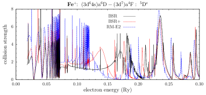
Figure 7: Predictions from two calculations Zatsarinny and Bartschat (2005); Ramsbottom et al. (2002) for the ${}^{5}D^{e}$ partial-wave collision strength of the electron-induced transition $(3d^{6}4s)^{6}D-(3d^{7})^{4}F$ in Fe⁺.

Comparing results from individual calculations makes little sense in this case. Instead, one should concentrate on an observable that is more stable regarding small changes in the individual predictions, but which is still meaningful in modeling applications. Such an observable is the effective collision strength, where an integral over the incident energies weighted over a Maxwellian (or possibly other) speed distribution is performed for a range of temperatures. An example is shown in figure 8. Comparing the results from different models should give some indication about the uncertainty of the predictions, especially if some additional criteria regarding the likely quality of the target description and the collision model are used to give increasing weight to a particular set of results. In the example shown, however, the latter may not even be necessary if an uncertainty of about 20% is deemed sufficient.

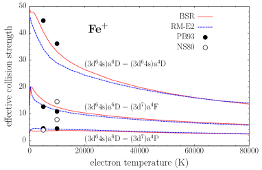
Figure 8: Predictions from a number of calculations for effective collision strengths as a function of temperature for electron collisions with Fe⁺. BSR results Zatsarinny and Bartschat (2005) are compared with those of Nussbaumer and Storey (NS80) Nussbaumer and Storey (1980), Pradhan and Berrington (PB93) Pradhan and Berrington (1993), and Ramsbottom et al. Ramsbottom et al. (2002).

For highly charged ions, as electron correlation effects are less important, perturbative methods such as PWBA, DWBA produce comparable results to nonperturbative methods as long as the structure description is reliable. As seen from figure 9, even for a singly-ionized system such as Be⁺, there is much better agreement between predictions from a number of different distorted-wave models and highly sophisticated close-coupling theories than between any of these predictions with the only available set of experimental data Falk and Dunn (1983). Given the importance of beryllium and its ions for fusion devices, additional calculations were recently performed, all of which essentially confirmed the results published in Colgan et al. (2003). The principal reason for this good agreement is the generally fast convergence of pseudo-state models with the number of pseudo-states included in the close-coupling expansion Mitnik et al. (1999). It is hence very likely that the theoretical results are more reliable than the experimental data in this case.

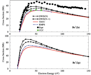
Figure 9: Electron impact ionization cross sections for Be⁺ from the $(2s)$ ground state and the $(2p)$ excited states. The predictions from several distorted-wave and close-coupling models are compared with the experimental data of Falk and Dunn Falk and Dunn (1983). (Figure adapted from Colgan et al. (2003).)

We note that cross sections, which are dominated by resonant processes, can be very sensitive to the details of the calculation. This has been explored, for example, for the e-C⁺ collision system Davey et al. (2000), where a single low-lying resonance dominates the low-energy behavior.

The process of dielectronic recombination is strongly affected by resonances and, moreover, an almost unbounded number of states and transitions can be involved. This makes it very difficult to calculate cross sections and even more difficult to estimate uncertainties in the calculated results. Experimental benchmarks are of the highest importance as may be seen in recent work for intermediate charge states of tungsten  Spruck et al. (2014); Badnell et al. (2016). However, in the recent article Badnell et al. (2015) there is a discussion of uncertainties in calculated rates of dielectronic recombination for S²⁺ recombining to S⁺ associated with uncertainties in the autoionizing level positions. The uncertainty was assessed by performing two additional calculations in which a critical autoionizing resonance position was shifted to just above threshold, thereby maximizing the resulting low-temperature rate coefficient, or by shifting it to an intermediate position. The authors conclude that “An observational program, combined with spectral modeling and a parallel effort in atomic theory, could make real progress in deriving DR rates for third and fourth row elements with well-defined uncertainties”.

VI.3 Electron-molecule collisions

Up until now, uncertainty assessment has been rare in electron-molecule collision calculations. An exception is the recent study of electron collisions with H${}_{2}^{+}$ by Zammit et al. Zammit et al. (2014). This system has the advantage that it is possible to use (near) exact wave functions for the one-electron target. Zammit et al. use a CCC technique and the adiabatic nuclei approximation to compute vibrationally resolved dissociative excitation and ionization cross sections for the system; they obtain results accurate to better than 10% and 5%, respectively. These uncertainty estimates were derived from considering (a) the behavior as function of the size of the CC expansion and (b) a smaller contribution due to their approximate treatment of nuclear motion. It would seem that the use of extended close-coupling expansions is the most promising approach for obtaining uncertainty quantified results for electron-molecule collisions.

The first example of the uncertainty assessment in electron-molecule collisions is the calculation of cross section for photodetachment of the C₂H^- anion. The analytical model used in the theoretical treatment of the process is described in ref. Douguet et al. (2014). It should be stressed here that the model does not account for possible rovibrational resonances that could be present in the photodetachment spectrum. Such a model would correspond to a low-resolution experiment, similar to the one of ref. Best et al. (2011), where rovibrational structure is unresolved. Figure 10 shows results of the theoretical calculations using the UK R-matrix code Tennyson (2010); Tennyson et al. (2007); Carr et al. (2012) with different values of several parameters, which control the accuracy of the electron scattering matrix obtained in the R-matrix code. The figure also shows the results of the complex Kohn method (see details in ref. Douguet et al. (2014)) and the available experimental data Best et al. (2011). Although a systematic uncertainty analysis of the calculation has not been performed, the R-matrix results shown in the figure suggest that the accuracy of the computation model is of the order of 15% for the cross section far from the electronic resonance at $4$ eV. The uncertainty in the position of the resonance is about $\pm 0.15$ eV. The present uncertainty analysis does not address the uncertainty of the analytical model itself that neglects the mentioned rovibrational resonances. However, in an ideal theoretical study of this or a similar process, the uncertainty of the analytical model should also be discussed.

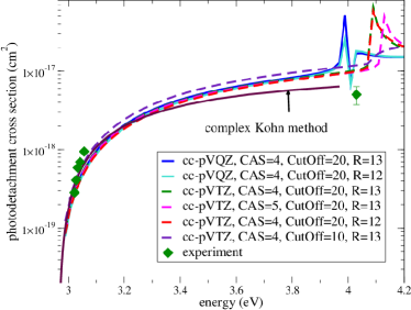
Figure 10: Theoretical (curves) Khamesian et al. (2016) and experimental (symbols) Best et al. (2011) cross sections for C₂H^- photodetachment. One of the shown theoretical curves is obtained using the complex Kohn method Douguet et al. (2014), all other curves are from the UK R-matrix Tennyson (2010); Tennyson et al. (2007) calculations. The R-matrix results are obtained for different values of key parameters controlling accuracy of electron scattering calculations at a fixed molecular geometry. Uncertainty of R-matrix and complex Kohn results is about 20% for the cross section far from the electronic resonance at $4$ eV.

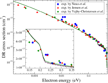
Figure 11: Theoretical (curves) and experimental (symbols) Vejby-Christensen et al. (1997); Neau et al. (2000); Jensen et al. (2000) cross section of dissociative recombination of the H₃O⁺ ion with electrons. There are three theoretical curves on the figure that are almost indistinguishable in the main graph. The inset zooms a part of the presented data such that three curves are distinguishable. Uncertainty of calculation within the employed analytical model (discussed in detail in ref. Douguet et al. (2012a)) is about 8%. Uncertainty of the analytical model itself is much larger because the model neglects some important physics, such as autoionization and rovibrational resonances present in the DR spectrum.

The second example is the cross section for dissociative recombination of the H₃O⁺ ion with low energy electrons. The analytical and computational model for the process is described in ref. Douguet et al. (2012a). Although the DR process also involves electron scattering, the employed model is very different from the one discussed above: the scattering matrix for collisions between an electron and a molecular ion in this approach is obtained from ab initio calculations of excited Rydberg states of the neutral H₃O molecule. Energies of the lowest electronic state of H₃O⁺ and several excited electronic states $E_{n}$ of H₃O are obtained using the Columbus code Shepard et al. (2008) (see details in Douguet et al. (2012a)). As a second step, effective quantum numbers $\nu_{n}({\cal Q})$ of the excited states are computed from energy difference $\Delta E_{n}({\cal Q})$ between H₃O⁺ and H₃O energies, where $\cal Q$ refers to a particular molecular geometry. Functions $\nu_{n}({\cal Q})$ are fit with a simple linear (or quadratic) function along $\cal Q$ and coefficients of the linear (or quadratic) fit are used to obtain the electron-molecule scattering matrix electron energies and, therefore, determine the final DR cross section. The electron-molecule scattering matrix for positive (relative to the ionization threshold) electronic energies is therefore computed from negative energies of Rydberg states in the spirit of quantum defect theory. In principle, Rydberg states with different principal quantum numbers $n$ could be used to perform the fit, to construct the scattering matrix, and to calculate the DR cross section. In theory, quantum defects $\mu_{n}=n-\nu_{n}$ are slightly different for different $n$, i.e. they are energy-dependent. Additional uncertainty of $\mu_{n}$ comes from the accuracy of the ab initio calculation. These are the two major sources of uncertainty in the calculation of the DR cross section within the discussed analytical model. The effect of these uncertainties on the final DR cross section is demonstrated in figure 11, where the cross section is calculated for three different sets of parameters obtained from three different manifolds of Rydberg states of H₃O. The difference in the results on the figure is attributed to accuracy of ab initio energies of excited electronic states of H₃O and to the energy dependence of the quantum defects. As in the first example, there is an additional source of uncertainty due to the employed analytical model, which neglects several possible processes during a DR event, such as the possibility of autoionization once the electron is captured by the ion or the influence of rovibrational resonances. This uncertainty is not addressed here.

VI.4 Charge transfer collisions

We begin the discussion of examples for uncertainty estimates in charge transfer collisions with the one-electron C${}^{6+}-{\rm H}(1s$) system. This and similar fully stripped ion - neutral hydrogen atom collision systems have been the subject of a large number of theoretical investigations over many years. In part, this is due to their relevance for applications such as charge exchange recombination spectroscopy, which is an important tool for the diagnostics of fusion plasmas (see, for example, refs. Igenbergs et al. (2012); Jorge et al. (2014) and references therein). Another reason for the great interest in these systems is their benchmark character. Being true one-electron problems, model uncertainties can be kept to a minimum and convergence properties of different approaches, i.e. numerical uncertainties can be studied.

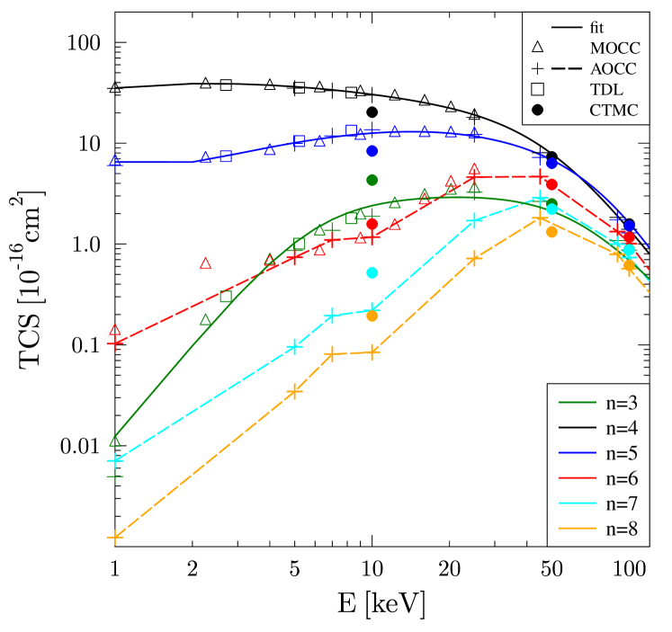
Figure 12: Cross sections for $n$-shell selective charge transfer in C⁶⁺-H($1s$) collisions as functions of impact energy. Full lines: fits according to Suno and Kato (2006), MOCC: Harel et al. (1998), AOCC: Igenbergs et al. (2012), TDL: Pindzola and Fogle (2015), CTMC: Cariatore et al. (2015).

Figure 12 displays cross sections for charge transfer from hydrogen into individual $n$-shells of the hydrogenlike C⁵⁺ ion in the low to intermediate energy regimes, in which the semiclassical approximation with straight-line trajectories is essentially exact. Based on a large set of cross section calculations carried out in the 1980s and 1990s, Suno and Kato constructed recommended data sets that can be fit by simple analytical functions Suno and Kato (2006). The recommended data are shown in figure 12 as solid lines. In addition, one recent representative is included for each of the following theoretical methods: MOCC Harel et al. (1998), AOCC Igenbergs et al. (2012), TDL Pindzola and Fogle (2015), and CTMC Cariatore et al. (2015). Experimental data on the $n$-shell resolved level are not available for this collision system.

It can be observed that predictions from the three semiclassical methods, MOCC, AOCC and TDL, are in excellent agreement with each other and with the recommended data for the dominant $n=4$ and the subdominant $n=5$ channels. From this comparison one can conclude that the cross section predictions are accurate to within a few percent. For the less important $n=3$ and $n=6$ channels the discrepancies are slightly larger. Except for the $n=6$ MOCC data point at 2 keV, however, the overall agreement is still very good.

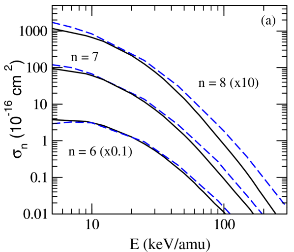
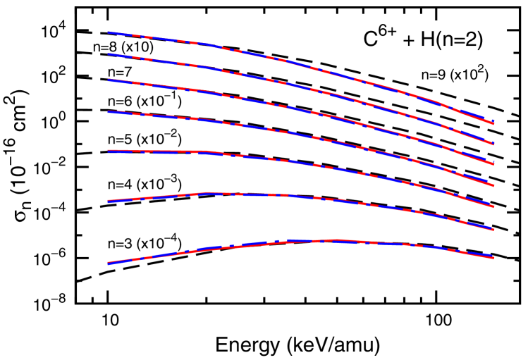
Figure 13: Cross sections for $n$-shell selective charge transfer in C${}^{6+}-{\rm H}(n\!=\!2$) collisions as functions of impact energy. Top panel: full lines: hydrogenic CTMC, dashed lines: AOCC. (Figure taken from Jorge et al. (2014).) Bottom panel: full lines: hydrogenic-Z-CTMC, dash-dotted lines: microcanonical CTMC (both sets of curves are essentially on top of each other), dashed lines: AOCC. (Figure taken from Cariatore et al. (2015).) The AOCC cross sections in both panels are from Igenbergs et al. (2012).

The CTMC results included in figure 12 agree very well with the semiclassical calculations at 50 and 100 keV impact energy. At lower energies the discrepancies are larger and different variants of CTMC models give different results Jorge et al. (2014); Cariatore et al. (2015). This suggests that an uncertainty assessment solely based on CTMC calculations would be difficult in this regime. However, at higher energies and for high $n$ quantum numbers the predictions of the different CTMC variants are all in good agreement with each other and can be viewed as the best results currently available.

Figure 13 shows $n$-shell specific charge transfer cross sections for C${}^{6+}-{\rm H}(n\!=\!2$) collisions. Due to the weaker binding of the electron in an excited initial state, higher projectile $n$-shells are favored, and overall the cross sections are larger when compared to the ground-state case. The CTMC calculations of Jorge et al. (top panel) and Cariatore et al. (bottom panel) appear to be in good agreement with each other, while the AOCC cross sections from ref. Igenbergs et al. (2012) tend to overestimate the CTMC data as the impact energy and the principal quantum number of the final states increase. Even though the two-center basis used includes a total of 340 states, which is a very large number for a semiclassical CC calculation, the overestimation is deemed to be a finite-basis effect, i.e. a convergence problem of the AOCC method in this energy range Jorge et al. (2014); Cariatore et al. (2015).

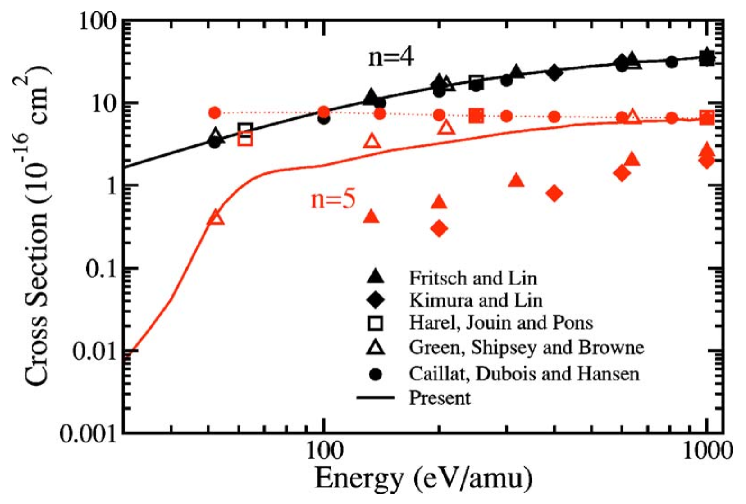
Figure 14: Cross sections for $n$-shell selective charge transfer in C⁶⁺-H($1s$) collisions as functions of impact energy. Full lines (“Present”): HSCC Liu et al. (2005); Fritsch and Lin: AOCC with curved trajectories Fritsch and Lin (1984); Kimura and Lin: (modified) AOCC with straight-line trajectories Kimura and Lin (1985); Harel et al.: MOCC with straight-line trajectories Harel et al. (1998); Green et al.: MOCC with curved trajectories Green et al. (1982a, b); Caillat et al.: AOCC with straight-line trajectories Caillat et al. (2000). (Figure taken from Liu et al. (2005).)

Figure 14 explores the very low energy regime in which straight-line trajectories, and perhaps the semiclassical approximation itself, become questionable. For the dominant $n=4$ channel in the C⁶⁺-H($1s$) collision system this does not appear to be an issue and semiclassical CC calculations based on curved and straight-line trajectories agree with each other and with a fully quantum mechanical HSCC calculation on the few-percent level. However, for $n=5$ qualitative discrepancies are observed. They have been traced to both basis-size limitations of the earlier CC calculations and to trajectory effects Caillat et al. (2000). Regarding the latter it was found that (i) straight-line trajectories lead to a strong overestimation of the cross section when the calculation is reasonably well converged with respect to basis size, and (ii) choosing the optimal curved trajectory involves a certain level of arbitrariness Caillat et al. (2000); Liu et al. (2005). The HSCC method is free of this ambiguity and probably gives the best answer. Interestingly, it is in close agreement with an early MOCC calculation, which used a relatively small number of states and curved trajectories based on an average molecular potential Green et al. (1982a, b). By contrast, a larger MOCC calculation based on straight-line trajectories yields significantly higher cross sections Harel et al. (1998). Given the absence of other fully quantum mechanical calculations and experimental data a quantitative uncertainty assessment appears to be difficult in this region.

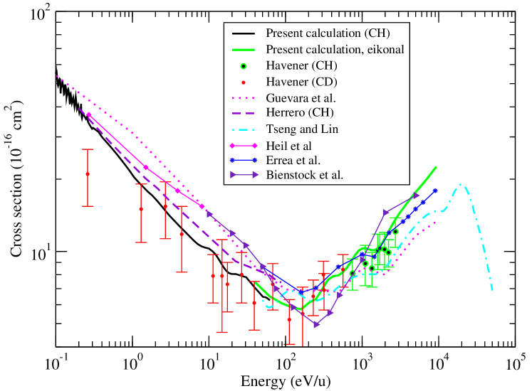
Figure 15: Total cross section for charge transfer in C³⁺-H($1s$) collisions as function of impact energy. “Present calculation (CH)”: QMOCC Errea et al. (2015); “Present calculation, eikonal”: MOCC Errea et al. (2015); Guevara et al.: END Guevara et al. (2011); Herrero (CH): QMOCC Herrero et al. (1995); Tseng and Lin: AOCC Tseng and Lin (1999); Heil et al.: QMOCC Heil et al. (1981); Errea et al.: MOCC Errea et al. (1991); Bienstock et al.: QMOCC Bienstock et al. (1982). Experimental data for atomic hydrogen [Havener (CH)] and deuterium [Havener (CD)]: Havener et al. (1995). (Figure taken from Errea et al. (2015).)

We now turn to single-electron transfer in the few-electron C${}^{3+}-{\rm H}(1s$) collision system. Figure 15 displays the total charge transfer cross section over a wide range of impact energies, spanning the very low energy, low energy, and intermediate energy regimes. A systematic trend can be observed at energies below 100 eV, which is where the cross section reaches a minimum. Of the four QMOCC calculations included the one that uses the most accurate correlated wave functions and the largest basis set (a total of ten many-electron molecular functions) gives the smallest cross section values and the best agreement with the experimental data. Except for the data point at the lowest energy of 0.3 eV/amu the calculated cross section curve lies within the experimental uncertainty. In the low energy region, in which the cross section increases with increasing impact energy, the convergence of molecular expansions slows down and above 2 keV/amu AOCC expansions are deemed to be more accurate Errea et al. (2015). This is supported by the close agreement of the calculations of refs. Tseng and Lin (1999); Guevara et al. (2011) with each other and, where available, with experimental data as well. Overall, figure 15 illustrates nicely that an uncertainty estimate for a complicated collision problem should use the input from several calculations based on different theoretical methods.

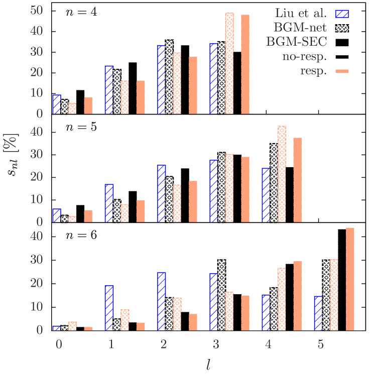
Figure 16: Relative cross sections for $nl$-subshell selective charge transfer in Ne¹⁰⁺-Ne collisions at 4.54 keV/amu. Liu et al.: AOCC Liu et al. (2014), all other results are from TC-BGM calculations Leung and Kirchner (2015). “BGM-net” and “BGM-SEC” refer to different statistical analyses of single transfer, while “resp” and “no-resp” calculations do or do not include a time-dependent response potential in the single-particle Hamiltonian. (Figure taken from Leung and Kirchner (2015).)

In figure 16 we show an example for single-electron transfer from a many-electron target. The system is 4.54 keV/amu Ne¹⁰⁺-Ne and plotted are relative cross sections for transfer into specific $nl$-subshells. Results from one AOCC and various TC-BGM calculations are included. All of them are on the level of the IEM, but they use different variants of effective target atom potentials and statistical methods for the calculation of the cross sections. It can be argued that what is referred to as BGM-SEC in the figure represents the most consistent calculation of single transfer within the IEM Leung and Kirchner (2015). However, this is no guarantee for success, since the IEM represents a model whose accuracy is difficult to determine. In lieu of correlated cross section calculations, comparing different IEM variants is the best one can do to assess the uncertainty of the theoretical results. A somewhat conservative estimate would then consist in taking the spread of the shown relative cross sections as their uncertainty.

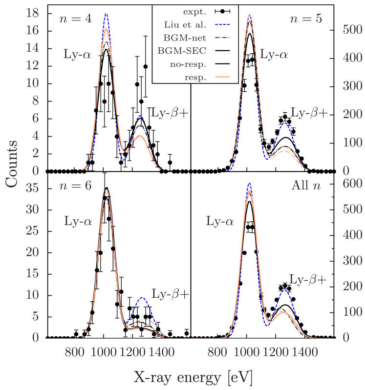
Figure 17: X-ray spectra from single electron transfer to the $n$-th shell in Ne¹⁰⁺-Ne collisions at 4.54 keV/amu. Experimental data: Ali et al. (2010); Liu et al.: AOCC Liu et al. (2014), all other results are from TC-BGM calculations (cf. figure 16) Leung and Kirchner (2015).

An important motivation for studying these $nl$-distributions is that they form the starting point for the calculation of x-ray spectra, which in turn are of interest, e.g., for the understanding of cometary x-ray emission. In figure 17 we show the modeled $n$-state selective spectra for the hydrogenlike Ne⁹⁺ ion produced in the charge transfer collision. Results from all calculations shown in figure 16 as well as experimental data from ref. Ali et al. (2010) are included. Overall, the spread in the theoretical x-ray spectra appears to be similar or even smaller than the spread in the relative cross sections, implying that error propagation is not problematic and the x-ray spectra are rather forgiving quantities. However, this is partly due to a mutual normalization process used in all of the calculations, and, perhaps to a lesser extent, to spectral-line convolutions to Gaussian profiles that were applied as well Leung and Kirchner (2015). The “widths” resulting from the various curves shown in figure 17 can again be taken as theoretical error bars.

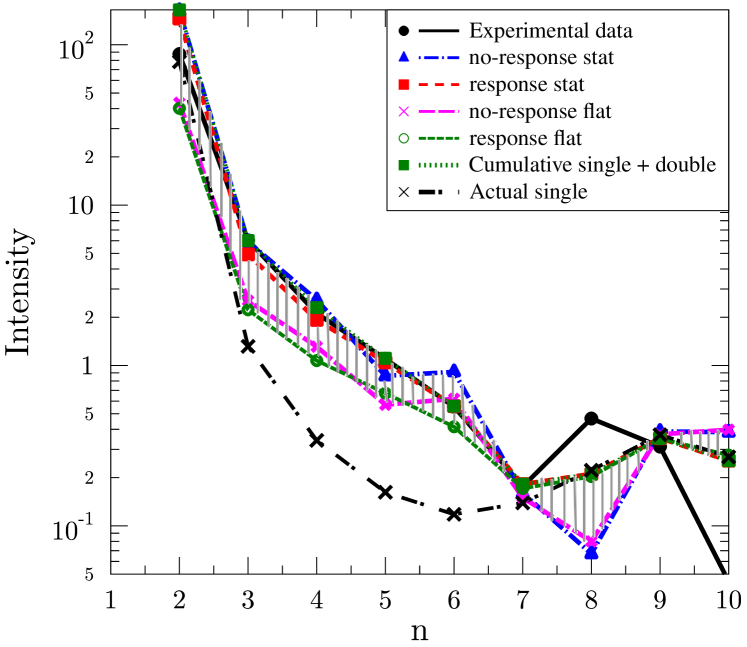
Figure 18: X-ray intensities after charge transfer in Ar¹⁷⁺-Ar collisions at 7 keV/amu. Experimental data: Trassinelli et al. (2012). All theoretical results are from TC-BGM calculations (see text) Salehzadeh and Kirchner (2013).

The last example of this section concerns a true many-electron problem: x-ray production after charge transfer in 7 keV/amu Ar¹⁷⁺-Ar collisions. In this case the available measurements Trassinelli et al. (2012) cannot discern single vs. multiple transfer. Given that the latter should be a strong channel for such a highly charged projectile ion, it has to be taken into account in the theoretical modeling of the measured x-ray spectra. In ref. Salehzadeh and Kirchner (2013) this was done on the level of the IEM, and again, different variants of effective potentials (response and no-response models) and statistical analyses were used in order to get a qualitative idea of the theoretical error bars. Further modeling is required in this problem to obtain x-ray emission spectra, because Auger processes compete with radiative de-excitation when multiple electron transfer occurs. Once again, different model variants were used for this (assuming flat vs. statistical $l$-subshell distributions after Auger electron emission) and the calculations were assessed by varying the models within reasonable bounds.

Figure 18 compares results obtained in this way with the experimental x-ray intensities for $1snp\rightarrow 1s^{2}$ transitions in the post-collision Ar¹⁶⁺ ion. One can probably take the shaded area as the theoretical error bar that results from the comparison of the different calculations. Except for $n=8$ and $n=10$ the experimental data are within these error bars. There is one calculation, however, that is clearly off. It represents an x-ray spectrum obtained from neglecting all multiple-transfer contributions in the calculation. This suggests that, despite considerable model uncertainties, some definite conclusions can be drawn from such calculations and comparisons; in this case, regarding the important role of multi-electron transfer events Salehzadeh and Kirchner (2013).

VII Summary, Conclusions, and Outlook

We have reviewed approaches to uncertainty estimates for atomic and molecular data of the kind that occur in plasma modeling. Model uncertainty is introduced through the treatment of small terms in the Hamiltonian and (more importantly in general) through the reduction of a many-body Schrödinger equation to a tractable model. Numerical uncertainty is due to the representation of the model on a finite mesh or basis. Uncertainties propagate from structure calculations to predictions of scattering cross sections. We have summarized the main tools for uncertainty assessment of calculations for atomic and (small molecule) molecular electronic structure, electron scattering, and charge transfer in heavy particle collisions. Important tools include the method of focal point analysis in connection with electronic structure models and, of course, standard methods of convergence analysis for the numerical uncertainties.

We discussed some examples of computational work on scattering calculations in which the authors attempted to provide a reasonable uncertainty estimate. These examples show that the field is not entirely unexplored. On the other hand, for every example of a scattering calculation that is accompanied by a thoroughly performed uncertainty estimate there are many more where the authors provide their best calculations without discussion of the uncertainties. For the case of electron impact collisions we discussed examples of atomic excitation and ionization where a reasonable uncertainty estimate is obtained by careful study of convergence in the structure calculation and in the R-matrix formalism.

Calculations of dielectronic recombination in electron-atom (ion) collisions are much more complicated than those of excitation and ionization, because very many states and transitions can be involved. Uncertainty estimates for calculated dielectronic recombination rate coefficients involve not just the convergence of the initial and final state structure, but also convergence with respect to the number of intermediate states and the number of transitions that are taken into account. As a consequence, for the dielectronic recombination process in electron-atom collisions the provision of uncertainties for calculated data (without relying on experimental benchmarks) is still wide open.

The ultimate aim for a constructive theory of uncertainty quantification for atomic and molecular data is to develop numerical procedures for structure and scattering calculations by which reasonable uncertainty estimates are obtained along with the primary calculated quantities of interest. The final quantities of interest are cross sections (differential cross sections in general) as a function of collision energy and perhaps other collision parameters. The associated uncertainties are structured quantities, not just point values, and they must be presented in a way that makes it possible to propagate them through further atomic data processing (e.g., to obtain effective rate coefficients) and through a plasma simulation. This raises many new issues that have not been addressed in this review, but that we note here as an outlook towards future work.

From an operational point of view, in order to propagate uncertainties in atomic data through a plasma simulation (in a non-intrusive manner, i.e., without major changes to the plasma simulation code) one needs to be able to sample the relevant cross sections with proper account of relevant correlations in uncertainties. For example, uncertainties in cross sections for the same process at different collision energies are correlated in some way that depends on the energies involved. Depending on the application such functional uncertainties (as opposed to pointwise uncertainties) may be represented by a Gaussian Process, a polynomial chaos expansion, or a Monte Carlo sample. The propagation of such uncertainties through a dynamical calculation is an issue of major interest in the field of Uncertainty Quantification as it is represented, for example, in the National Research Council report already cited in the Introduction National Research Council Committee on Mathematical Foundations of Verification, Validation, and Uncertainty Quantification (2012). For a perspective from Statistics on Uncertainty Quantification see also, O’Hagan (2013) and for a monograph-length treatment of Uncertainty Quantification with special attention to computational fluid dynamics see LeMaitre and Omar (2010).

In this review we have discussed the state of the art in uncertainty assessment for calculated atomic and molecular data for plasma applications. We conclude with what we regard as major issues for future work. First, very broadly, we recommend that atomic and molecular physicists develop methods and codes for scattering calculations in which uncertainty assessment is integrated with the calculation of the primary quantities of interest. Second, more narrowly, develop uncertainty assessment in a more systematic way for processes involving resonances: near-threshold processes and dielectronic recombination. Third, develop representations of correlated uncertainties in atomic and molecular data that are suitable for studies in which those uncertainties have to be propagated through plasma simulations. The latter item will benefit from a joint effort by atomic physicists and plasma modellers.

References

- The Editors (2011) The Editors, Phys. Rev. A 83, 040001 (2011).
- National Research Council Committee on Mathematical Foundations of Verification, Validation, and Uncertainty Quantification (2012) National Research Council Committee on Mathematical Foundations of Verification, Validation, and Uncertainty Quantification, Assessing the reliability of complex models: mathematical and statistical foundations of verification, validation and uncertainty quantification (National Academies Press, 2012).
- (3) http://www.siam.org/activity/uq/.
- Dirac (1929) P. A. M. Dirac, Proc. R. Soc. A 123, 714 (1929).
- IAE (2014) (2014), https://www-amdis.iaea.org/meetings/ITAMP/.
- Sto (2015) (2015), http://www.iacs.stonybrook.edu/uq/pages/workshop.
- Reiter and Janev (2010) D. Reiter and R. K. Janev, Contrib. Plasma Phys. 50, 986 (2010).
- Császár et al. (1998) A. G. Császár, W. D. Allen, and H. F. Schaefer III, J. Chem. Phys. 108, 9751 (1998).
- Boyarkin et al. (2013) O. V. Boyarkin, M. A. Koshelev, O. Aseev, P. Maksyutenko, T. R. Rizzo, N. F. Zobov, L. Lodi, J. Tennyson, and O. L. Polyansky, Chem. Phys. Lett. 568-â569, 14 (2013).
- berto Capote and Smith (2008) berto Capote and D. L. Smith, Nuclear Data Sheets 109, 2768 (2008).
- Bethe and Salpeter (1957) H. A. Bethe and E. E. Salpeter, Quantum Mechanics Of One- And Two-Electron Atoms (Springer-Verlag, Berlin, 1957) pp. 4 – 46.
- Eides et al. (2001) M. I. Eides, H. Grotch, and V. A. Shelyuto, Phys. Rep. 342, 63 (2001).
- Jentschura et al. (2005) U. D. Jentschura, S. Kotochigova, E.-O. Le Bigot, P. J. Mohr, and B. N. Taylor, Phys. Rev. Lett. 95, 163003 (2005).
- Pachucki and Jentschura (2003) K. Pachucki and U. D. Jentschura, Phys. Rev. Lett. 91, 113005 (2003).
- Yerokhin and Shabaev (2015) V. A. Yerokhin and V. M. Shabaev, J. Phys. Chem. Ref. Data 44, 033103 (2015).
- Gumberidze et al. (2011) A. Gumberidze, T. Stöhlker, D. Banaś, H. Beyer, C. Brandau, H. Bräuning, S. Geyer, S. Hagmann, S. Hess, P. Indelicato, et al., Hyperfine Interact. 199, 59 (2011).
- Klahn and Bingel (1977) B. Klahn and W. Bingel, Theor. Chim. Acta 44, 27 (1977).
- Klahn and Bingel (1978) B. Klahn and W. Bingel, Int. J. Quantum Chem. 11, 943 (1978).
- Schwartz (2006) C. Schwartz, Int. J. Mod. Phys. E–Nucl. Phys. 15, 877 (2006).
- Nakashima and Nakatsuji (2007) H. Nakashima and H. Nakatsuji, J. Chem. Phys. 127, 224104 (2007).
- Drake and Yan (1992) G. W. F. Drake and Z.-C. Yan, Phys. Rev. A 46, 2378 (1992).
- Korobov (2000) V. I. Korobov, Phys. Rev. A 61, 064503 (2000).
- Bailey (1993) D. Bailey, ACM Trans. Math. Softw. 19, 288 (1993).
- Bailey (1995) D. Bailey, ACM Trans. Math. Softw. 379, 21 (1995), see also http://crd-legacy.lbl.gov/ dhbailey/mpdist/.
- Drake et al. (2002) G. Drake, M. Cassar, and R. Nistor, Phys. Rev. A 65, 054501 (2002).
- Wang et al. (2012) L. Wang, Z. Yan, H. Qiao, and G. Drake, Phys. Rev. A 85, 052513 (2012).
- Drake and Martin (1998) G. W. F. Drake and W. C. Martin, Can. J. Phys. 76, 679 (1998).
- Morton et al. (2006) D. C. Morton, Q.-X. Wu, and G. W. F. Drake, Can. J. Phys. 84, 83 (2006).
- Yan et al. (2008a) Z. C. Yan, W. Noertershaeuser, and G. W. F. Drake, Phys. Rev. Lett. 100, 243002 (2008a).
- Yerokhin and Pachucki (2010) V. A. Yerokhin and K. Pachucki, Phys. Rev. A 81, 022507 (2010).
- Drake (2006) G. W. F. Drake, in Handbook of Atomic, Molecular, and Optical Physics, edited by G. W. F. Drake (Springer-Verlag, New York, 2006) Chap. 11.
- Drake (1988) G. W. F. Drake, Can. J. Phys. 66, 586 (1988).
- Artemyev et al. (2005) A. N. Artemyev, V. M. Shabaev, V. A. Yerokhin, G. Plunien, and G. Soff, Phys. Rev. A 71, 062104 (2005).
- Chantler et al. (2010) C. T. Chantler, J. Lowe, and I. Grant, Phys. Rev. A 82, 052505 (2010).
- Fischer (2014) C. F. Fischer, Atoms 2, 1 (2014).
- Träbert (2014) E. Träbert, Atoms 2, 15 (2014).
- Kramida (2014) A. Kramida, Atoms 2, 86 (2014).
- Ekman et al. (2014) J. Ekman, M. R. Godefroid, and H. Hartman, Atoms 2, 215 (2014).
- Kelleher (2014) D. E. Kelleher, Atoms 2, 382 (2014).
- Safronova et al. (2014a) M. S. Safronova, V. A. Dzuba, V. V. Flambaum, U. I. Safronova, S. G. Porsev, and M. G. Kozlov, Phys. Rev. A 90, 042513 (2014a).
- Safronova et al. (2014b) M. S. Safronova, V. A. Dzuba, V. V. Flambaum, U. I. Safronova, S. G. Porsev, and M. G. Kozlov, Phys. Rev. A 90, 052509 (2014b).
- Kállay et al. (2011) M. Kállay, H. S. Nataraj, B. K. Sahoo, B. P. Das, and L. Visscher, Phys. Rev. A 83, 030503 (2011).
- Fischer (2009) C. F. Fischer, Phys. Scr. 2009, 014019 (2009).
- Born and Oppenheimer (1927) M. Born and J. R. Oppenheimer, Ann. Phys. 84, 457 (1927).
- Born and Huang (1954) M. Born and K. Huang, Dynamical Theory of Crystal Lattice (Clarendon Press, 1954).
- Zobov et al. (1996) N. F. Zobov, O. L. Polyansky, C. R. Le Sueur, and J. Tennyson, Chem. Phys. Lett. 260, 381 (1996).
- Polyansky and Tennyson (1999) O. L. Polyansky and J. Tennyson, J. Chem. Phys. 110, 5056 (1999).
- Diniz et al. (2013) L. G. Diniz, J. R. Mohallem, A. Alijah, M. Pavanello, L. Adamowicz, O. L. Polyansky, and J. Tennyson, Phys. Rev. A 88, 032506 (2013).
- E. Mt́yus and Császár (2014) T. S. E. Mt́yus and A. G. Császár, The Journal of Chemical Physics 141, 154111 (2014).
- Császár et al. (2000) A. G. Császár, W. D. Allen, Y. Yamaguchi, and H. F. Schaefer III, in Computational Molecular Spectroscopy (Wiley, New York, 2000) pp. 15–68.
- Császár et al. (2001) A. G. Császár, G. Tarczay, M. L. Leininger, O. L. Polyansky, J. Tennyson, and W. D. Allen, in In: Spectroscopy from space (Kluwer, Dordrecht, 2001) pp. 17–339.
- Yamaguchi et al. (1994) Y. Yamaguchi, Y. Osamura, J. D. Goddard, and H. F. Schaefer, A New Dimension to Quantum Chemistry: Analytic Derivative Methods in Ab Initio Molecular Electronic Structure Theory (International Series of Monographs on Chemistry) (Oxford University Press, 1994).
- Murrell et al. (1984) J. N. Murrell, S. Carter, S. C. Farantos, P. Huxley, and A. J. C. Varandas, Molecular Potential Energy Surfaces (Wiley, New York, 1984).
- Braams and Bowman (2009) B. J. Braams and J. M. Bowman, Int. Rev. Phys. Chem. 28, 577 (2009).
- Tarczay et al. (2001) G. Tarczay, A. G. Császár, W. Klopper, and H. M. Quiney, Mol. Phys. 99, 1769 (2001).
- Dunning (1989) T. H. Dunning, Jr., J. Chem. Phys. 90, 1007 (1989).
- Császár and Allen (1996) A. G. Császár and W. D. Allen, J. Chem. Phys. 104, 2746 (1996).
- Pyykkö et al. (2001) P. Pyykkö, K. G. Dyall, A. G. Császár, G. Tarczay, O. L. Polyansky, and J. Tennyson, Phys. Rev. A 63, 024502 (2001).
- Lodi et al. (2008) L. Lodi, R. N. Tolchenov, J. Tennyson, A. E. Lynas-Gray, S. V. Shirin, N. F. Zobov, O. L. Polyansky, A. G. Császár, J. van Stralen, and L. Visscher, J. Chem. Phys. 128, 044304 (2008).
- Lodi et al. (2011) L. Lodi, J. Tennyson, and O. L. Polyansky, J. Chem. Phys. 135, 034113 (2011).
- Jensen (2006) F. Jensen, Introduction to Computational Chemistry (Wiley, New York, 2006).
- Lipiński (2002) J. Lipiński, Chem. Phys. Lett. 363, 313 (2002).
- Werner et al. (1983) H. J. Werner, P. Rosmus, and E. A. Reinsch, J. Chem. Phys. 79, 905 (1983).
- Ernzerhof et al. (1992) M. Ernzerhof, C. M. Marian, and S. D. Peyerimhoff, Intern. J. Quantum Chem. 43, 659 (1992).
- Lodi and Tennyson (2010) L. Lodi and J. Tennyson, J. Phys. B: At. Mol. Opt. Phys. 43, 133001 (2010).
- Pindzola and Kelly (1975) M. S. Pindzola and H. P. Kelly, Phys. Rev. A 12, 1419 (1975).
- Griffin et al. (2009) D. C. Griffin, C. P. Ballance, and M. S. Pindzola, Phys. Rev. A 80, 023420 (2009).
- Adamson et al. (1998) S. O. Adamson, A. Zaitsevskii, and N. F. Stepanov, J. Phys. B: At. Mol. Opt. Phys. 31, 5275 (1998).
- Lodi et al. (2015) L. Lodi, S. N. Yurchenko, and J. Tennyson, Mol. Phys. 113, 1559 (2015).
- McKemmish et al. (2016) L. K. McKemmish, S. N. Yurchenko, and J. Tennyson, J. Chem. Theory Comput. (2016).
- Tennyson et al. (2016) J. Tennyson, L. Lodi, L. K. McKemmish, and S. N. Yurchenko, J. Phys. B: At. Mol. Opt. Phys. (2016), topical Review.
- Jain and Gianturco (1991) A. Jain and F. Gianturco, J. Phys. B: At. Mol. Opt. Phys. 24, 2387 (1991).
- Jones and Tennyson (2010) M. Jones and J. Tennyson, J. Phys. B: At. Mol. Opt. Phys. 43, 045101 (2010).
- Brigg et al. (2014) W. J. Brigg, J. Tennyson, and M. Plummer, J. Phys. B: At. Mol. Opt. Phys. 47, 185203 (2014).
- Jonsson et al. (1997) D. Jonsson, P. Norman, and H. Agren, Chem. Phys. 224, 201 (1997).
- DeYonker et al. (2014) N. DeYonker, D. Halfen, W. Allen, and L. Ziurys, J. Chem. Phys. 141, 204302 (2014).
- Valeev et al. (2001) E. Valeev, W. Allen, H. Schaefer, A. Császár, and A. East, Journal of Physical Chemistry A 105, 2716 (2001).
- Bokareva et al. (2009) O. Bokareva, V. Bataev, V. Pupyshev, and I. Godunov, Spectrochim. Acta Mol. Biomol. Spectrosc. 73, 654 (2009).
- Little and Tennyson (2013) D. A. Little and J. Tennyson, J. Phys. B: At. Mol. Opt. Phys. 46, 145102 (2013).
- Jungen (1996) C. Jungen, ed., Molecular Applications of Quantum Defect Theory (Taylor and Francis, 1996).
- Tennyson (1996) J. Tennyson, J. Phys. B: At. Mol. Opt. Phys. 29, 6185 (1996).
- Schneider et al. (2000) I. F. Schneider, I. Rabadán, L. Carata, J. Tennyson, L. H. Andersen, and A. Suzor-Weiner, J. Phys. B: At. Mol. Opt. Phys. 33, 4849 (2000).
- Cocks et al. (2010) D. G. Cocks, I. B. Whittingham, and G. Peach, J. Phys. B: At. Mol. Opt. Phys. 43, 135102 (2010).
- Bartschat (2013) K. Bartschat, J. Phys. D: Appl. Phys. 46, 334004 (2013).
- Bartschat and Zatsarinny (2015) K. Bartschat and O. Zatsarinny, Phys. Scr. 90, 054006 (2015).
- Burke (2011) P. G. Burke, R-Matrix Theory of Atomic Collisions: Application to Atomic, Molecular and Optical Processes (Springer, 2011).
- Tennyson (2010) J. Tennyson, Phys. Rep. 491, 29 (2010).
- Bray et al. (2012) I. Bray, D. Fursa, A. Kadyrov, A. Stelbovics, A. Kheifets, and A. Mukhamedzhanov, Phys. Rep. 520, 135 (2012), electron- and photon-impact atomic ionisation.
- Bartschat et al. (1996) K. Bartschat, E. T. Hudson, M. P. Scott, P. G. Burke, and V. M. Burke, J. Phys. B: At., Mol. Opt. Phys. 29, 115 (1996).
- Gorfinkiel and Tennyson (2004) J. D. Gorfinkiel and J. Tennyson, J. Phys. B: At. Mol. Opt. Phys. 37, L343 (2004).
- Colgan et al. (2002) J. Colgan, M. S. Pindzola, F. J. Robicheaux, D. C. Griffin, and M. Baertschy, Phys. Rev. A 65, 042721 (2002).
- Rescigno et al. (1999) T. N. Rescigno, M. Baertschy, W. A. Isaacs, and C. W. McCurdy, Science 286, 2474 (1999).
- Taylor (1972) J. R. Taylor, Scattering theory (Wiley, 1972).
- Joachain (1984) C. J. Joachain, Quantum collision theory (Elsevier Science Ltd, 1984).
- Madison and Shelton (1973) D. Madison and W. Shelton, Phys. Rev. A 7, 499 (1973).
- Itikawa (1986) Y. Itikawa, Phys. Rep. 143, 69 (1986).
- Bote and Salvat (2008) D. Bote and F. Salvat, Phys. Rev. A 77, 042701 (2008).
- Gao et al. (2006) J. F. Gao, D. H. Madison, and J. L. Peacher, J. Phys. B: At. Mol. Opt. Phys. 39, 1275 (2006).
- Al-Hagan et al. (2009) O. Al-Hagan, C. Kaiser, D. Madison, and A. J. Murray, Nature Phys. 5, 59 (2009).
- Toth and Nagy (2011) I. Toth and L. Nagy, J. Phys. B: At. Mol. Opt. Phys. 44, 195205 (2011).
- Zhang et al. (2014) S. B. Zhang, X. Y. Li, J. G. Wang, Y. Z. Qu, and X. Chen, Phys. Rev. A 89, 052711 (2014).
- Badnell (2008) N. Badnell, J. Phys. B: At., Mol. Opt. Phys. 41, 175202 (2008).
- Fursa and Bray (2008) D. V. Fursa and I. Bray, Phys. Rev. Lett. 100, 113201 (2008).
- Zuo et al. (1991) T. Zuo, R. McEachran, and A. Stauffer, J. Phys. B: At., Mol. Opt. Phys. 24, 2853 (1991).
- Kim (2001) Y.-K. Kim, Phys. Rev. A 64, 032713 (2001).
- Kim and Rudd (1994) Y.-K. Kim and M. E. Rudd, Phys. Rev. A 50, 3954 (1994).
- Laporta et al. (2012) V. Laporta, C. M. Cassidy, J. Tennyson, and R. Celiberto, Plasma Sources Sci. Technol. 21, 045005 (2012).
- Laporta et al. (2015) V. Laporta, R. Celiberto, and J. Tennyson, Phys. Rev. A 91, 012701 (2015).
- Chang and Fano (1972) E. Chang and U. Fano, Phys. Rev. A 6, 173 (1972).
- Morrison et al. (1984) M. A. Morrison, A. N. Feldt, and B. C. Saha, Phys. Rev. A 30, 2811 (1984).
- Atabek et al. (1974) O. Atabek, D. Dill, and C. Jungen, Phys. Rev. Lett. 33, 123 (1974).
- Greene and Ch.Jungen (1985) C. H. Greene and Ch.Jungen, Adv. At. Mol. Phys. 21, 51 (1985).
- Seaton (1966) M. J. Seaton, Proc. Phys. Soc. London 88, 801 (1966).
- Aymar et al. (1996) M. Aymar, C. H. Greene, and E. Luc-Koenig, Rev. Mod. Phys. 68, 1015 (1996).
- Greene et al. (1979) C. Greene, U. Fano, and G. Strinati, Phys. Rev. A 19, 1485 (1979).
- Gao and Greene (1989) H. Gao and C. H. Greene, J. Chem. Phys. 91, 3988 (1989).
- Gao and Greene (1990) H. Gao and C. H. Greene, Phys. Rev. A 42, 6946 (1990).
- Sun et al. (1995) W. Sun, M. A. Morrison, W. A. Isaacs, W. K. Trail, D. T. Alle, R. Gulley, M. J. Brennan, and S. J. Buckman, Phys. Rev. A 52, 1229 (1995).
- Chase (1956) D. M. Chase, Phys. Rev. 104, 838 (1956).
- Faure et al. (2009a) A. Faure, V. Kokoouline, C. H. Greene, and J. Tennyson, J. Phys. Conf. Ser. 192, 012016 (2009a).
- Faure et al. (2009b) A. Faure, J. Tennyson, V. Kokoouline, and C. H. Greene, J. Phys. Conf. Ser. 192, 012016 (2009b).
- Kokoouline et al. (2010) V. Kokoouline, A. Faure, J. Tennyson, and C. H. Greene, Mon. Not. R. Astron. Soc. 405, 1195 (2010).
- Norcross and Padial (1982) D. W. Norcross and N. T. Padial, Phys. Rev. A 25, 226 (1982).
- Sanna and Gianturco (1998) N. Sanna and F. A. Gianturco, Comput. Phys. Commun. 114, 142 (1998).
- O’Malley (1966) T. F. O’Malley, Phys. Rev. 150, 14 (1966).
- Bates (1991) D. R. Bates, J. Phys. B: At., Mol. Opt. Phys. 24, 695 (1991).
- Guberman and Giusti-Suzor (1991) S. L. Guberman and A. Giusti-Suzor, J. Chem. Phys. 95, 2602 (1991).
- Morgan and Noble (1984) L. A. Morgan and C. J. Noble, J. Phys.B: At. Mol. Phys. 17, L369 (1984).
- Fujimoto et al. (2012) M. M. Fujimoto, W. J. Brigg, and J. Tennyson, Eur. Phys. J. D 66, 204 (2012).
- Bardsley (1967) J. Bardsley, Chem. Phys. Lett. 1, 229 (1967).
- Kokoouline et al. (2011) V. Kokoouline, N. Douguet, and C. H. Greene, Chem. Phys. Lett. 507, 1 (2011).
- Douguet et al. (2012a) N. Douguet, A. E. Orel, C. H. Greene, and V. Kokoouline, Phys. Phys. Lett. 108 (2012a).
- Douguet et al. (2012b) N. Douguet, V. Kokoouline, and A. E. Orel, J. Phys. B: At. Mol. Opt. Phys. 45, 051001 (2012b).
- Fonseca dos Santos et al. (2014) S. Fonseca dos Santos, N. Douguet, V. Kokoouline, and A. Orel, J. Chem. Phys. 140, 164308 (2014).
- Little et al. (2014) D. A. Little, K. Chakrabarti, I. F. Schneider, and J. Tennyson, Phys. Rev. A 90, 052705 (2014).
- Faure and Tennyson (2002) A. Faure and J. Tennyson, J. Phys. B: At. Mol. Opt. Phys. 35, 1865 (2002).
- Kokoouline and Greene (2003a) V. Kokoouline and C. H. Greene, Phys. Rev. Lett. 90, 133201 (2003a).
- Kokoouline and Greene (2003b) V. Kokoouline and C. H. Greene, Phys. Rev. A 68, 012703 (2003b).
- Jungen and Pratt (2008a) C. Jungen and S. T. Pratt, J. Chem. Phys. 129, 164310 (2008a).
- Jungen and Pratt (2008b) C. Jungen and S. T. Pratt, J. Chem. Phys. 129, 164311 (2008b).
- Jungen and Pratt (2009) C. Jungen and S. T. Pratt, Phys. Rev. Lett. 102, 023201 (2009).
- Gorfinkiel and Tennyson (2005) J. D. Gorfinkiel and J. Tennyson, J. Phys. B: At. Mol. Opt. Phys. 38, 1607 (2005).
- Halmová and Tennyson (2008) G. Halmová and J. Tennyson, Phys. Rev. Lett. 100, 213202 (2008).
- Pindzola et al. (2012) M. S. Pindzola, S. A. Abdel-Naby, J. A. Ludlow, F. Robicheaux, and J. Colgan, Phys. Rev. A 85 (2012).
- Colgan and Pindzola (2012) J. Colgan and M. S. Pindzola, Eur. Phys. J. D 66, 284 (2012).
- Gao et al. (2005) J. F. Gao, D. H. Madison, and J. L. Peacher, J. Chem. Phys. 123, 204314 (2005).
- Kaiser et al. (2007) C. Kaiser, D. Spieker, J. Gao, M. Hussey, A. Murray, and D. H. Madison, J. Phys. B: At. Mol. Opt. Phys. 40, 2563 (2007).
- Bransden and McDowell (1992) B. H. Bransden and M. R. C. McDowell, Charge Exchange and the Theory of Ion-Atom Collisions (Clarendon Press, Oxford, 1992).
- Belkić (2008) D. Belkić, Quantum Theory of High-Energy Ion-Atom Collisions (CRC Press, Boca Raton, 2008).
- Loreau et al. (2014) J. Loreau, S. Ryabchenko, and N. Vaeck, J. Phys. B 47, 135204 (2014).
- Delos (1981) J. B. Delos, Rev. Mod. Phys. 53, 287 (1981).
- Errea et al. (1994) L. F. Errea, C. Harel, H. Jouin, L. Méndez, B. Pons, and A. Ríera, J. Phys. B 27, 3603 (1994).
- Liu et al. (2005) C.-N. Liu, S.-C. Cheng, A.-T. Le, and C. D. Lin, Phys. Rev. A 72, 012717 (2005).
- Zygelman et al. (1997) B. Zygelman, P. C. Stancil, N. J. Clarke, and D. L. Cooper, Phys. Rev. A 56, 457 (1997).
- Li et al. (2015) T. C. Li, Y. Z. Qu, Y. Wu, L. Liu, J. G. Wang, H.-P. Liebermann, and R. J. Buenker, Phys. Rev. A 91, 052702 (2015).
- Abdurakhmanov et al. (2016) I. B. Abdurakhmanov, A. S. Kadyrov, and I. Bray, J. Phys. B 49, 03LT01 (2016).
- Deumens et al. (1994) E. Deumens, A. Diz, R. Longo, and Y. Öhrn, Rev. Mod. Phys. 66, 917 (1994).
- Cabrera-Trujillo (2010) R. Cabrera-Trujillo, Plasma Sources Sci. Technol. 19, 034006 (2010).
- Green et al. (1982a) T. A. Green, E. J. Shipsey, and J. C. Browne, Phys. Rev. A 25, 1364 (1982a).
- Green et al. (1982b) T. A. Green, M. E. Riley, E. J. Shipsey, and J. C. Browne, Phys. Rev. A 26, 3668 (1982b).
- Fritsch and Lin (1984) W. Fritsch and C. D. Lin, Phys. Rev. A 29, 3039 (1984).
- van Hemert et al. (1985) M. C. van Hemert, E. F. van Dishoeck, J. A. van der Hart, and F. Koike, Phys. Rev. A 31, 2227 (1985).
- Fritsch and Lin (1991) W. Fritsch and C. D. Lin, Phys. Rep. 202, 1 (1991).
- Zapukhlyak et al. (2005) M. Zapukhlyak, T. Kirchner, H. J. Lüdde, S. Knoop, R. Morgenstern, and R. Hoekstra, J. Phys. B 38, 2353 (2005).
- Kuang and Lin (1997) J. Kuang and C. D. Lin, J. Phys. B 30, 101 (1997).
- Kroneisen et al. (1999) O. J. Kroneisen, H. J. Lüdde, T. Kirchner, and R. M. Dreizler, J. Phys. A 32, 2141 (1999).
- Minami et al. (2006) T. Minami, M. S. Pindzola, T.-G. Lee, and D. R. Schultz, J. Phys. B 39, 2877 (2006).
- Pindzola and Fogle (2015) M. S. Pindzola and M. Fogle, J. Phys. B 48, 205203 (2015).
- Belkić et al. (2008) D. Belkić, I. Manc̆ev, and J. Hanssen, Rev. Mod. Phys. 80, 249 (2008).
- Niehaus (1986) A. Niehaus, J. Phys. B 19, 2925 (1986).
- Olson and Salop (1977) R. E. Olson and A. Salop, Phys. Rev. A 16, 531 (1977).
- Otranto et al. (2014) S. Otranto, N. D. Cariatore, and R. E. Olson, Phys. Rev. A 90, 062708 (2014).
- Sánchez et al. (2006) R. Sánchez, W. Nörtershäuser, G. Ewald, D. Albers, J. Behr, P. Bricault, B. A. Bushaw, A. Dax, J. Dilling, M. Dombsky, G. W. F. Drake, S. Götte, R. Kirchner, H.-J. Kluge, T. Kühl, J. Lassen, C. D. P. Levy, M. R. Pearson, E. J. Prime, V. Ryjkov, A. Wojtaszek, Z.-C. Yan, and C. Zimmermann, Phys. Rev. Lett. 96, 033002 (2006).
- Sanchez et al. (2009) R. Sanchez, M. Zakova, Z. Andjelkovic, B. A. Bushaw, K. Dasgupta, G. Ewald, C. Geppert, H.-J. Kluge, J. Kraemer, M. Nothhelfer, D. Tiedemann, D. F. A. Winters, and W. Noertershaeuser, New J. Phys. 11 (2009).
- Yan et al. (2008b) Z.-C. Yan, W. Nörtershäuser, and G. W. F. Drake, Phys. Rev. Lett. 100, 243002 (2008b), erratum: Phys. Rev. Lett. 102, 249903 (2009).
- Yan et al. (2009) Z.-C. Yan, W. Nörtershäuser, and G. W. F. Drake, Phys. Rev. Lett. 102, 249903 (2009).
- Puchalski et al. (2010) M. Puchalski, D. Kedziera, and K. Pachucki, Phys. Rev. A 82, 062509 (2010).
- Yan and Drake (2003) Z.-C. Yan and G. W. F. Drake, Phys. Rev. Lett. 91, 113004 (2003).
- Nörtershäuser et al. (2011) W. Nörtershäuser, R. Sánchez, G. Ewald, A. Dax, J. Behr, P. Bricault, B. A. Bushaw, J. Dilling, M. Dombsky, G. W. F. Drake, S. Götte, H.-J. Kluge, T. Kühl, J. Lassen, C. D. P. Levy, K. Pachucki, M. Pearson, M. Puchalski, A. Wojtaszek, Z.-C. Yan, and C. Zimmermann, Phys. Rev. A 83, 012516 (2011).
- Lu et al. (2013) Z.-T. Lu, P. Mueller, G. W. F. Drake, W. Nörtershäuser, S. C. Pieper, and Z.-C. Yan, Rev. Mod. Phys. 85, 1383 (2013).
- Puzzarini et al. (2008) C. Puzzarini, M. Heckert, and J. Gauss, J. Chem. Phys. 128, 194108 (2008).
- Demaison et al. (2010) J. Demaison, J. E. Boggs, and A. G. Csaszar, Equilibrium Molecular Structures: From Spectroscopy to Quantum Chemistry (CRC Press, Boca Raton, 2010).
- Makarov et al. (2015) D. S. Makarov, M. A. Koshelev, N. F. Zobov, and O. V. Boyarkin, Chem. Phys. Lett. 627, 73 (2015).
- Polyansky et al. (2015) O. L. Polyansky, K. Bielska, M. Ghysels, L. Lodi, N. F. Zobov, J. T. Hodges, and J. Tennyson, Phys. Rev. Lett. 114, 243001 (2015).
- Lodi and Tennyson (2012) L. Lodi and J. Tennyson, J. Quant. Spectrosc. Radiat. Transf. 113, 850 (2012).
- Zak et al. (2016) E. Zak, J. Tennyson, O. L. Polyansky, L. Lodi, S. A. Tashkun, and V. I. Perevalov, J. Quant. Spectrosc. Radiat. Transf. (2016).
- Elford (2000) M. T. Elford, “Photon and Electron Interactions with Atoms, Molecules, and Ions (Landolt-Börnstein: Numerical Data and Functional Relationships in Science and Technology / Elementary Particles, Nuclei and Atoms),” (Springer, New York, 2000).
- Trajmar (1973) S. Trajmar, Phys. Rev. A 8, 191 (1973).
- Hall et al. (1972) R. I. Hall, G. Joyez, Y. Mazeau, J. Reinhard, and C. Schermann, J. Physique 34, 827 (1972).
- Donaldson et al. (1972) F. G. Donaldson, M. A. Hender, and J. W. McConkey, J. Phys. B: At., Mol. Phys. 5, 1192 (1972).
- Fursa and Bray (1995) D. V. Fursa and I. Bray, Phys. Rev. A 52, 1279 (1995).
- Bartschat (1998) K. Bartschat, J. Phys. B: At., Mol. Opt. Phys. 31, L469 (1998).
- Zatsarinny et al. (2014) O. Zatsarinny, Y. Wang, and K. Bartschat, Phys. Rev. A 89, 022706 (2014).
- Boffard et al. (1999) J. B. Boffard, G. A. Piech, M. F. Gehrke, L. W. Anderson, and C. C. Lin, Phys. Rev. A 59, 2749 (1999).
- Hibbert (1975) A. Hibbert, Comp. Phys. Commun. 9, 141 (1975).
- Eissner et al. (1974) W. Eissner, M. Jones, and H. Nussbaumer, Comp. Phys. Commun. 8, 270 (1974).
- Zatsarinny and Bartschat (2005) O. Zatsarinny and K. Bartschat, Phys. Rev. A 72, 020702 (2005).
- Ramsbottom et al. (2002) C. A. Ramsbottom, M. P. Scott, K. L. Bell, F. P. Keenan, B. M. McLaughlin, A. G. Sunderland, V. M. Burke, C. J. Noble, and P. G. Burke, J. Phys. B: At., Mol. Opt. Phys. 35, 3451 (2002).
- Nussbaumer and Storey (1980) H. Nussbaumer and P. J. Storey, Astron. Astrophys. 89, 308 (1980).
- Pradhan and Berrington (1993) A. K. Pradhan and K. A. Berrington, J. Phys. B 26, 157 (1993).
- Falk and Dunn (1983) R. A. Falk and G. H. Dunn, Phys. Rev. A 27, 754 (1983).
- Colgan et al. (2003) J. Colgan, S. D. Loch, M. S. Pindzola, C. P. Ballance, and D. C. Griffin, Phys. Rev. A 68, 032712 (2003).
- Mitnik et al. (1999) D. M. Mitnik, M. S. Pindzol, , D. C. Griffin, and N. R. Badnell, 32, L479 (1999).
- Davey et al. (2000) A. R. Davey, P. J. Storey, and R. Kisielius, Astron. Astrophys. Suppl. Ser. 142, 85 (2000).
- Spruck et al. (2014) K. Spruck, N. R. Badnell, C. Krantz, O. Novotny, A. Becker, D. Bernhardt, and M. G. et al., Phys. Rev. A 90, 032715 (2014).
- Badnell et al. (2016) N. R. Badnell, K. Spruck, C. Krantz, O. Novotny, A. Becker, D. Bernhardt, and M. G. et al, Phys. Rev. A 93, 052703 (2016).
- Badnell et al. (2015) N. R. Badnell, G. J. Ferland, T. W. Gorczyca, D. Nikoli., and G. A. Wagle, The Astrophysical Journal 804, 100 (2015).
- Zammit et al. (2014) M. C. Zammit, D. V. Fursa, and I. Bray, Phys. Rev. A 90, 022711 (2014).
- Douguet et al. (2014) N. Douguet, V. Kokoouline, and A. E. Orel, Phys. Rev. A 90, 063410 (2014).
- Best et al. (2011) T. Best, R. Otto, S. Trippel, P. Hlavenka, A. von Zastrow, S. Eisenbach, S. Jezouin, R. Wester, E. Vigren, M. Hamberg, and W. D. Geppert, Astrophys. J. 742, 63 (2011).
- Tennyson et al. (2007) J. Tennyson, D. B. Brown, J. J. Munro, I. Rozum, H. N. Varambhia, and N. Vinci, J. Phys. Conf. Ser. 86, 012001 (2007).
- Carr et al. (2012) J. M. Carr, P. G. Galiatsatos, J. D. Gorfinkiel, A. G. Harvey, M. A. Lysaght, D. Madden, Z. Masin, M. Plummer, and J. Tennyson, Eur. Phys. J. D 66, 58 (2012).
- Khamesian et al. (2016) M. Khamesian, N. Douguet, S. Fonseca dos Santos, O. Dulieu, M. Raoult, and V. Kokoouline, Eur. Phys. J. D , Submitted (2016).
- Vejby-Christensen et al. (1997) L. Vejby-Christensen, L. Andersen, O. Heber, D. Kella, H. Pedersen, H. Schmidt, and D. Zajfman, Astrophys. J. 483, 531 (1997).
- Neau et al. (2000) A. Neau, A. A. Khalili, S. Rosén, A. L. Padellec, A. M. Derkatch, W. Shi, L. Vikor, M. Larsson, J. Semaniak, R. Thomas, M. B. Någård, K. Andersson, H. Danared, and M. af Ugglas, J. Chem. Phys. 113, 1762 (2000).
- Jensen et al. (2000) M. J. Jensen, R. C. Bilodeau, C. P. Safvan, K. Seiersen, L. H. Andersen, H. B. Pedersen, and O. Heber, Astrophys. J. 543, 764 (2000).
- Shepard et al. (2008) R. Shepard, I. Shavitt, R. M. Pitzer, M. Dallos, T. Müller, P. G. Szalay, F. B. Brown, R. Ahlrichs, H. J. Böhm, A. Chang, D. C. Comeau, R. Gdanitz, H. Dachsel, C. Ehrhardt, M. Ernzerhof, P. Höchtl, S. Irle, G. Kedziora, T. Kovar, V. Parasuk, M. J. M. Pepper, P. Scharf, H. Schiffer, M. Schindler, M. Schüler, M. Seth, E. A. Stahlberg, J.-G. Zhao, S. Yabushita, Z. Zhang, M. Barbatti, S. Matsika, M. Schuurmann, D. R. Y. S. R. Brozell, E. V. Beck, H. Lischka, M. Ruckenbauer, B. Sellner, F. Plasser, J.-P. Blaudeau, and J. J. Szymczak, “Columbus,” (2008), columbus, an ab initio electronic structure program, release 5.9.2 (2008).
- Igenbergs et al. (2012) K. Igenbergs, J. Schweinzer, A. Veiter, L. Perneczky, E. Frühwirth, M. Wallerberger, R. E. Olson, and F. Aumayr, J. Phys. B 45, 065203 (2012).
- Jorge et al. (2014) A. Jorge, L. F. Errea, C. Illescas, and L. Méndez, Eur. Phys. J. D 68, 227 (2014).
- Suno and Kato (2006) H. Suno and T. Kato, At. Data Nucl. Data Tables 92, 407 (2006).
- Harel et al. (1998) C. Harel, H. Jouin, and B. Pons, At. Data Nucl. Data Tables 68, 279 (1998).
- Cariatore et al. (2015) N. D. Cariatore, S. Otranto, and R. E. Olson, Phys. Rev. A 91, 042709 (2015).
- Kimura and Lin (1985) M. Kimura and C. D. Lin, Phys. Rev. A 32, 1357 (1985).
- Caillat et al. (2000) J. Caillat, A. Dubois, and J. P. Hansen, J. Phys. B 33, L715 (2000).
- Errea et al. (2015) L. F. Errea, C. Illescas, A. Jorge, L. Méndez, I. Rabadán, and J. Suárez, J. Phys.: Conf. Ser. 576, 012002 (2015).
- Guevara et al. (2011) N. L. Guevara, E. Teixeira, B. Hall, Y. Öhrn, E. Deumens, and J. R. Sabin, Phys. Rev. A 83, 052709 (2011).
- Herrero et al. (1995) B. Herrero, I. L. Cooper, A. S. Dickinson, and D. R. Flower, J. Phys. B 28, 711 (1995).
- Tseng and Lin (1999) H. C. Tseng and C. D. Lin, J. Phys. B 32, 5271 (1999).
- Heil et al. (1981) T. G. Heil, S. E. Butler, and A. Dalgarno, Phys. Rev. A 23, 1100 (1981).
- Errea et al. (1991) L. F. Errea, B. Herrero, L. Méndez, and A. Ríera, J. Phys. B 24, 4061 (1991).
- Bienstock et al. (1982) S. Bienstock, T. G. Heil, C. Bottcher, and A. Dalgarno, Phys. Rev. A 25, 2850 (1982).
- Havener et al. (1995) C. C. Havener, A. Müller, P. A. Zeijlmans van Emmichoven, and R. A. Phaneuf, Phys. Rev. A 51, 2982 (1995).
- Liu et al. (2014) L. Liu, J. G. Wang, and R. K. Janev, Phys. Rev. A 89, 012710 (2014).
- Leung and Kirchner (2015) A. C. K. Leung and T. Kirchner, Phys. Rev. A 92, 032712 (2015).
- Ali et al. (2010) R. Ali, P. A. Neill, P. Beiersdörfer, C. L. Harris, D. R. Schultz, and P. C. Stancil, Astrophys. J. Lett. 716, L95 (2010).
- Trassinelli et al. (2012) M. Trassinelli, C. Prigent, E. Lamour, F. Mezdari, J. Mérot, R. Reuschl, J.-P. Rozet, S. Steydli, and D. Vernhet, J. Phys. B 45, 085202 (2012).
- Salehzadeh and Kirchner (2013) A. Salehzadeh and T. Kirchner, J. Phys. B 46, 025201 (2013).
- O’Hagan (2013) A. O’Hagan, Polynomial chaos: A tutorial and critique from a statistician.s perspective (SIAM/ASA J. Uncertainty Quantification, 2013) http://www.tonyohagan.co.uk/academic/pdf/Polynomial-chaos.pdf.
- LeMaitre and Omar (2010) O. P. LeMaitre and M. K. Omar, Spectral methods for uncertainty quantification (Springer, New York, 2010).