Uplink FBMC/OQAM-based Multiple Access Channel: Distortion Analysis
under Strong Frequency Selectivity

Abstract

This paper computes the distortion power at the receiver side of an FBMC/OQAM-based OFDMA uplink channel under strong frequency selectivity and/or user timing errors. More precisely, it provides a distortion expression that is valid for a wide class of prototype pulses (not necessarily perfect-reconstruction ones) when the number of subcarriers is sufficiently large. This result is a valuable instrument for analyzing how users interfere to one another and to justify, formally, the common choice of placing an empty guard band between adjacent users. Interestingly, the number of out-band subcarriers contaminated by each user only depends on the prototype pulses and not on the channel nor on the equalizer. To conclude, the distortion analysis presented in this paper, together with some simulation results for a realistic scenario, also provide convincing evidence that FBMC/OQAM-based OFDMA is superior to classic circular-prefix OFDMA in the case of asynchronous users.

I Introduction

Multicarrier techniques are based on the idea that a frequency-selective channel can be split into a number of flat orthogonal subchannels. As a result, sophisticated channel equalization schemes can be replaced by simple (typically one-tap) per-subcarrier equalizers. For this reason, both wired (e.g., digital subscriber line, powerline communications) and wireless (e.g., WiFi, WiMAX) communications systems have long been employing multicarrier strategies in order to control Intersymbol Interference (ISI) while limiting complexity [1].

Recently, established communications standards like LTE have based also their multiple access features on a multicarrier approach [2]. Besides simple equalization, multicarrier transmission offers a flexible mechanism to dynamically allocate variable portions of the spectrum to users, according to their throughput requirements and the channel response. Theoretically, it consists in a trivial assignment of subcarriers to users. In practice, however, things may become substantially more complicated, depending on the synchronization requirements between users and Base Station (BS) and, especially, among different users.

In [3], M. Morelli et al. analyze the synchronization problem for the Orthogonal Frequency Division Multiple Access (OFDMA) scheme, which is probably the most common multicarrier multiple-access strategy based on an extension of the well-known Circular Prefix Orthogonal Frequency Multiplexing (CP-OFDM) scheme. The authors highlight the fact that, similarly to CP-OFDM, OFDMA suffers from poor spectrum containment and is hence very sensitive to frequency offsets. The issue is exacerbated in the uplink, since synchronism is needed among signals at the receiver side (and not at the transmitters). Timing- and frequency-tracking algorithms are presented in [3], together with interference-cancellation procedures that are required to remove residual interference. The resulting receiver is thus a complex system and the inherent efficiency loss caused by the presence of the CP is not justified anymore.

Filterbank Multicarrier (FBMC) modulation is an old technique (see, e.g., [4]) that is regaining popularity in the last few years as a potential solution to the efficiency and synchronization limitations of CP-OFDM and CP-OFDMA [5, 6]. In FBMC, orthogonality among subchannels is obtained by means of well-designed filters with low side lobes, and is much less sensitive to frequency offsets as shown in, e.g., [7]. Furthermore, no CP is needed, thus improving the spectral efficiency. One should be aware, however, that one-tap per-subcarrier equalizers are not ideal anymore (especially in highly frequency selective channels) and more sophisticated solutions are often needed [8, 9, 10, 11]. For this reason, and because of FBMC architectures being more complex than their CP-OFDM counterparts, FBMC is still not very popular in point-to-point communications. On the other hand, the complexity gap cancels out (or possibly reverses) in multiple-access scenarios, as discussed above (see, e.g., [12, 13]). For instance, users do not need to be synchronized since the timing at each subcarrier can be corrected separately.

This paper considers a frequency selective multiple-access uplink channel as the one depicted in Fig. 1 and characterizes the distortion of the received symbols assuming an FBMC/OQAM-based OFDMA scheme. Users are not synchronized and their channels towards the BS are highly frequency selective. No particular hypothesis is formulated about the FBMC prototype pulses, while a single-tap per-subcarrier equalizer is implemented. We mentioned before that this equalizer is suboptimal; however, a rigorous mathematical analysis of more sophisticated receiver architectures would result in extremely complex derivations. Moreover, single-tap equalizers are often used in real practical systems due to their simplicity.

The resulting distortion is thus the joint effect of suboptimal equalization and a “poor” filter choice. As opposed to other works, where an empirical approach is preferred [12, 14], the analysis below is based on a tight approximation that accurately represents the received signal when the number of subcarriers is large enough. This approximation is based on the results of [11] and follows similar lines. It is worth remarking, however, that the problem at hand presents some specific difficulties that cannot be seen as simple extensions of [11]. Indeed, important properties of the involved operations [e.g., of the Discrete Fourier Transform (DFT)] do not hold when the spectrum is not considered in its integrity, but is split among the different users.

A fine characterization of the distortion brings valuable help with the design of an FBMC-based OFDMA system. Each user contributes not only to the distortion at its assigned subcarriers (in-band distortion), but also at other users’ subcarriers (out-band distortion). Indeed, the interference caused by frequency selective channels, inherent to FBMC schemes, is exacerbated in the multiple user case since all users undergo different channels, whose combined effect may be unpredictable. The purpose of this analysis is to confirm the intuition that, with sharp prototype pulses, leaving one empty subcarrier as a guard-band is sufficient [14, 15]. Moreover, it also applies to prototype pulses that are not so frequency selective, like those used in double-dispersive channels and designed to optimize the time–frequency localization of the waveform [16, 7, 17, 18]. Luckily, according to the results below, the number of subcarriers affected by the out-band leakage only depends on the prototype pulses at both sides of the FBMC links. Conversely, channel responses, equalizer and synchronization misalignments only affect the distortion magnitude. This means that no channel state information is needed to choose the prototype pulses that minimize the leakage effect or to decide whether one or more empty guard-bands are needed between users.

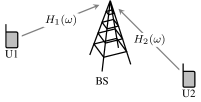
Figure 1: An uplink frequency selective multiple-access channel with two users.

The rest of the paper is organized as follows. Section II provides the model for the FBMC-based OFDMA channel under consideration while recalling basic concepts of FBMC modulation. Then, the derivation and the interpretation of the distortion approximation are reported in Section III. Finally, Section IV contains some numerical assessment of the results and Section V concludes the paper.

Notation

Hereafter, lowercase (respectively, uppercase) boldface letters denote column vectors (respectively, matrices). Occasionally, matrices that are functions of other matrices are denoted by uppercase calligraphic letters. Superscripts $(\cdot)^{*}$, $(\cdot)^{T}$ and $(\cdot)^{H}$ represent complex conjugate, transpose and complex (Hermitian) transpose, respectively. For a generic matrix $\mathbf{A}$, $[\mathbf{A}]_{k,l}$ is its $(k,l)$ entry. Also, borrowing from Matlab${}^{\text{\textregistered}}$ notation, $[\mathbf{A}]_{:,l}$ and $[\mathbf{A}]_{k,:}$ denote the $l$-th column and the $k$-th row of $\mathbf{A}$, respectively. The entries of the diagonal matrix $\operatorname{diag}\{\mathbf{a}\}$ (respectively, $\operatorname{diag}_{n=1,\dots,N}\{a_{n}\}$) are the elements of vector $\mathbf{a}$ (respectively, of the sequence $a_{1},\dots,a_{N}$). $\operatorname{tr}A$ stands for the trace of matrix $\mathbf{A}$. $\operatorname{\mathbb{R}e}\{\mathbf{A}\}$ and $\operatorname{\mathbb{I}m}\{\mathbf{A}\}$ are the real and imaginary parts of $\mathbf{A}$, so that $\mathbf{A}=\operatorname{\mathbb{R}e}\{\mathbf{A}\}+\mathrm{j}\operatorname{\mathbb{I}m}\{\mathbf{A}\}$, with $\mathrm{j}$ the imaginary unit. The operators $\otimes$, $\odot$ and $\circledast$ stand for Kronecker product, Hadamard (element-wise) product and row-wise convolution, respectively (matrix dimension restrictions apply), while $\operatorname{\mathbb{E}}[\cdot]$ is the expected value. Symbol $\mathbf{0}_{m,n}$ (respectively, $\mathbf{1}_{m,n}$) denotes an $m\times n$ matrix with all entries equal to 0 (respectively, to 1). For simplicity, subscripts may be removed (i.e., $\mathbf{0}$ and $\mathbf{1}$) from column vectors whose length can be clearly determined by the context. Finally, $\mathbf{I}_{k}$ and $\mathbf{J}_{k}$ represent the $k\times k$ identity and anti-identity (with one-valued entries only on the main anti-diagonal) matrix, respectively.

II Signal Model

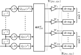
Figure 2: Block diagram of an FBMC/OQAM-based OFDMA receiver assuming that subcarriers are equally split between two users. Blocks labeled “de-stag.” represent the de-staggering operation (see, e.g., [11]). The coefficients of the polyphase filters $Q_{m}(z^{-2})=\sum_{n=1}^{\kappa}q_{N}[m+2(n-1)M]z^{-2(n-1)}$ are given by the $m$-th row of matrix $\mathbf{Q}$.

In this paper we focus on an OFDMA channel obtained by means of an FBMC modulation based on Offset Quadrature Amplitude Modulation (FBMC/OQAM, also known as staggered modulated multitone). More precisely, we are interested in the uplink channel where a common sink (e.g., a BS) receives data from $K$ users (the case of two users is depicted in Fig. 1): each user is assigned a subset of the available $2M$ equally spaced subcarriers, according to some allocation policy. Let $\mathcal{I}_{k}$ denote the set of subcarrier indices reserved for user $k$, so that $\bigcup_{k=1}^{K}\mathcal{I}_{k}=\{1,\dots,2M\}$ and $\mathcal{I}_{k}\cap\mathcal{I}_{k^{\prime}}=\emptyset$ for all $k^{\prime}\neq k$. Since channel and receiver are linear systems, the received signal can be written as the sum of user contributions. Then, for user $k$, let $\mathbf{A}_{k}=\mathbf{B}_{k}+\mathrm{j}\mathbf{C}_{k}$ be the $2M\times N_{s}$ matrix representing a block of $N_{s}$ multicarrier QAM symbols: for all $n=1,\dots,N_{s}$ and all $m\in\mathcal{I}_{k}$, entries $[\mathbf{B}_{k}]_{m,n}$ and $[\mathbf{C}_{k}]_{m,n}$ are independent (of one another and across $k$, $m$ and $n$) real-valued bounded random variables with zero mean and finite variance. Conversely, for $m\notin\mathcal{I}_{k}$, the entries of $\mathbf{A}_{k}$ are identically null.

II-A Memoryless Channel

Let $p_{N}[n]$ and $q_{N}[n]$ be the real prototype pulses at the transmitter side and at the receiver side, respectively. The length of both pulses is $N=2M\kappa$ taps, where the overlapping factor $\kappa$ is an integer value. From the prototype pulses we can build matrices

$$\mathcal{R}(p_{N},q_{N}) =\begin{bmatrix}\mathbf{P}_{1}\circledast\mathbf{J}_{M}\mathbf{Q}_{2}\\ \mathbf{P}_{2}\circledast\mathbf{J}_{M}\mathbf{Q}_{1}\end{bmatrix}$$ (1)

$$\mathcal{S}(p_{N},q_{N}) =\begin{bmatrix}\mathbf{P}_{2}\circledast\mathbf{J}_{M}\mathbf{Q}_{2}\\ \mathbf{P}_{1}\circledast\mathbf{J}_{M}\mathbf{Q}_{1}\end{bmatrix}$$ (2)

where $\mathbf{P}_{1}$ and $\mathbf{P}_{2}$ gather the top half and the bottom half rows, respectively, of matrix

$$\mathbf{P}=\begin{bmatrix}\mathbf{P}_{1}\\ \mathbf{P}_{2}\end{bmatrix}=\begin{bmatrix}p_{N}[1]&\cdots&p_{N}[2M(\kappa-1)+1]\\ \vdots&&\vdots\\ p_{N}[2M]&\cdots&p_{N}[2M\kappa]\end{bmatrix}.$$

Note that the $m$-th row of $\mathbf{P}$ contains the coefficients of the $m$-th Type-I polyphase component of the prototype pulse $p_{N}[n]$. Equivalently, matrix $\mathbf{Q}={\begin{bmatrix}\mathbf{Q}_{1}^{T}&\mathbf{Q}_{2}^{T}\end{bmatrix}}^{T}$ is the polyphase representation of the receiver prototype pulse $q_{N}[n]$.

For an ideal (memoryless and noiseless) channel, the output of the analysis filterbank corresponding to signal $\mathbf{A}_{k}$ (see Fig. 2) can be written as

$$\mathbf{Y}_{k}(p_{N},q_{N})=\mathbf{Y}_{k}^{\text{even}}(p_{N},q_{N})\otimes[1,0]+\mathbf{Y}_{k}^{\text{odd}}(p_{N},q_{N})\otimes[0,1]$$

where

$$\mathbf{Y}_{k}^{\text{odd}}(p_{N},q_{N})=2\mathbf{\Phi}\mathbf{F}_{2M}^{H}\Bigl{(}[\mathbf{F}_{2M}\mathbf{\Phi}^{*}\mathbf{B}_{k},\mathbf{0},\mathbf{0}]\circledast\mathcal{R}(p_{N},q_{N})\Bigr{)}$$

$${}+2\mathbf{\Phi}\mathbf{F}_{2M}^{H}\Biggl{(}\begin{bmatrix}\mathbf{0},\mathrm{j}\mathbf{G}_{2}\mathbf{\Phi}^{*}\mathbf{C}_{k},\mathbf{0}\\ \mathrm{j}\mathbf{G}_{1}\mathbf{\Phi}^{*}\mathbf{C}_{k},\mathbf{0},\mathbf{0}\end{bmatrix}\circledast\mathcal{S}(p_{N},q_{N})\Biggr{)},$$ (3a)

$$\mathbf{Y}_{k}^{\text{even}}(p_{N},q_{N})=2\mathbf{\Phi}\mathbf{F}_{2M}^{H}\Bigl{(}[\mathbf{0},\mathrm{j}\mathbf{F}_{2M}\mathbf{\Phi}^{*}\mathbf{C}_{k},\mathbf{0}]\circledast\mathcal{R}(p_{N},q_{N})\Bigr{)}$$

$${}+2\mathbf{\Phi}\mathbf{F}_{2M}^{H}\Biggl{(}\begin{bmatrix}\mathbf{0},\mathbf{G}_{2}\mathbf{\Phi}^{*}\mathbf{B}_{k},\mathbf{0}\\ \mathbf{G}_{1}\mathbf{\Phi}^{*}\mathbf{B}_{k},\mathbf{0},\mathbf{0}\end{bmatrix}\circledast\mathcal{S}(p_{N},q_{N})\Biggr{)}.$$ (3b)

and where we have introduced the diagonal matrix $\mathbf{\Phi}=\operatorname{diag}_{m=1,\dots,2M}\Bigl{\{}\exp\Bigl{[}-\mathrm{j}\pi\frac{M+1}{2M}(m-1)\Bigr{]}\Bigr{\}}$ and the $2M\times 2M$ Fourier matrix $\mathbf{F}_{2M}$ with entries $[\mathbf{F}_{2M}]_{m,n}=(2M)^{-1/2}\exp\Bigl{[}\mathrm{j}\frac{2\pi}{2M}(m-1)(n-1)\Bigr{]}$. The upper (respectively, lower) $M$ rows of $\mathbf{F}_{2M}$ are denoted by $\mathbf{G}_{1}$ (respectively, $\mathbf{G}_{2}$), so that $\mathbf{F}_{2M}={\begin{bmatrix}\mathbf{G}_{1}^{T}&\mathbf{G}_{2}^{T}\end{bmatrix}}^{T}$. Equation (3) is the input–output FBMC/OQAM signal model according to the efficient polyphase implementation [16, 11]. It is worth remarking that, even though based on the polyphase formulation, the results below characterize the distortion for all the equivalent implementations of the FBMC/OQAM architecture, namely the classical transmultiplexer implementation with complex modulated prototype pulses [16], the frequency-spreading formulation [19, 20] and, in some extent, the fast-convolution based FBMC [21].

As it can be evinced from (3), there exists a complex relationship between the transmitted symbols and the received ones. However, as proven in [16, 22, 11], for instance, message recovery is possible since

$${[\mathbf{A}_{k}]}_{m,n}=\operatorname{\mathbb{R}e}{[\mathbf{Y}_{k}^{\text{odd}}(p_{N},q_{N})]}_{m,n+\kappa-1}+\mathrm{j}\operatorname{\mathbb{I}m}{[\mathbf{Y}_{k}^{\text{even}}(p_{N},q_{N})]}_{m,n+\kappa}$$ (4)

whenever the prototype pulses meet the Perfect Reconstruction (PR) constraints

$$\mathbf{U}^{+}\mathcal{R}(p_{N},q_{N}) =\mathbb{I}$$ (5a)

$$\mathbf{U}^{-}\mathcal{S}(p_{N},q_{N}) =\mathbf{0}_{2M\times(2\kappa-1)}.$$ (5b)

Matrices $\mathbf{U}^{+}$ and $\mathbf{U}^{-}$ are defined as

$$\mathbf{U}^{\pm}=\mathbf{I}_{2}\otimes(\mathbf{I}_{M}\pm\mathbf{J}_{M})$$ (6)

while $\mathbb{I}=[\mathbf{0}_{2M\times(\kappa-1)},\mathbf{1},\mathbf{0}_{2M\times(\kappa-1)}].$

II-B Frequency-Selective Channel

As mentioned above, multicarrier modulations find their main application when the communication channel is frequency selective. In such a situation, however, the memoryless model in (3) does not hold anymore. Indeed, due to the delay spread, the received signal can be seen as a weighted combination of a number of delayed replicas. The delay and the weight of each replica depend on the channel impulse response. Note that timing errors between transmitter and receiver are covered by this model, since they are equivalent to a phase shift in the channel frequency response. Conversely, frequency offsets need a more sophisticated analysis that is not treated in this paper in order to avoid further complexity. In other words, we are assuming that channel estimations are refreshed often enough to neglect the Doppler effect.

Under a frequency selectivity assumption, a more useful approximation for the output of the analysis filterbank in Fig. 2 is given by [11]

$$\mathbf{Z}_{k}^{(*)}(p_{N},q_{N})=\mathbf{W}\mathbf{\Lambda}_{H_{k}}\mathbf{Y}_{k}^{(*)}(p_{N},q_{N})-\frac{\mathrm{j}}{2M}\mathbf{W}\mathbf{\Lambda}_{H_{k}^{(1)}}\mathbf{Y}_{k}^{(*)}\Bigl{(}p_{N},q_{N}^{(1)}\Bigr{)}\\ {}-\frac{1}{8M^{2}}\mathbf{W}\mathbf{\Lambda}_{H_{k}^{(2)}}\mathbf{Y}_{k}^{(*)}\Bigl{(}p_{N},q_{N}^{(2)}\Bigr{)}+\mathbf{o}\bigl{(}M^{-2}\bigr{)}$$ (7)

where $(*)\in\{\text{odd},\text{even}\}$ and where

• the diagonal matrix $\mathbf{W}$ collects the $2M$ coefficients of a channel equalizer with a single tap per subcarrier;

• the $m$-th entry of the diagonal matrix $\mathbf{\Lambda}_{H_{k}^{(r)}}$ is $H_{k}^{(r)}(\omega_{m})$, that is the value of the $r$-th derivative of the channel frequency response $H_{k}(\omega)$ computed at $\omega=\omega_{m}$, the central frequency of subcarrier $m$;

• the symbols $\mathbf{Y}_{k}^{(*)}\Bigl{(}p_{N},q_{N}^{(r)}\Bigr{)}$ are built as in (3) after substituting the receiver prototype pulse $q_{N}$ with its $r$-th derivative $q_{N}^{(r)}$ (see below);

• $\mathbf{o}\bigl{(}M^{-2}\bigr{)}$ represents a matrix of appropriate size whose entries decay faster than $M^{-2}$ as $M\to+\infty$.

The approximation in (7) is derived for an asymptotically large number $2M$ of subcarriers under the following assumptions.

AS1

The coefficients of $p_{N}[n]$ and $q_{N}[n]$ are uniformly bounded for $M\to+\infty$.

AS2

The pulse $q_{N}[n]=q_{N}^{(0)}[n]$ and its derivatives $q_{N}^{(r)}[n]$ are obtained according to

$$q_{N}^{(r)}[n]=T_{s}^{r}q^{(r)}\biggl{(}\biggl{(}n-\frac{N+1}{2}\biggr{)}\frac{T_{s}}{2M}\biggr{)},$$

where $T_{s}$ is the multicarrier symbol period in time units and where $q(t)$ is a twice continuously differentiable real function defined over $[-\kappa T_{s}/2,\kappa T_{s}/2]$. Moreover, the function and its first two derivatives null out at the boundary points of the domain, that is $q(\pm\kappa T_{s}/2)=q^{(1)}(\pm\kappa T_{s}/2)=q^{(2)}(\pm\kappa T_{s}/2)=0$. An example is depicted in Fig. 3.

Recall that the subcarrier bandwidth, and hence the multicarrier symbol duration, are kept constant. This means that, by increasing the number of subcarriers, we are considering a wider spectrum (or, equivalently, a higher sampling frequency). This assumption may seem not very practical; nevertheless, numerical results will show how asymptotic expressions finely approximate real systems with reasonable total bandwidth and number of subcarriers.

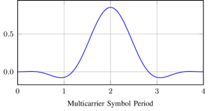
Figure 3: Prototype pulse defined by the EU-funded project PHYDYAS [23] with overlapping factor $\kappa=4$: it is a good approximation of a prototype pulse satisfying the required assumptions.

Even though the expansion in (7) can be easily extended to any order higher than two, the extra terms would not bring any significant contributions to the analysis below. Numerical results in Section IV will confirm this statement and the fact that (7) is representative of practical systems with a sufficiently large number of subcarriers. Similarly, more sophisticated equalizers (e.g., single-tap minimum mean square error or even more complex schemes like those described in [8, 9, 10, 11]) could be considered and included in our study. However, this choice would make the mathematical derivations extremely complicated and hard to follow.

III Distortion Analysis

III-A Preliminary considerations

Before delving into the analysis of the distortion affecting the considered system, we need to clarify how distortion is defined. Let us focus on subcarrier $m$ assigned to user $\ell$, i.e. $m\in\mathcal{I}_{\ell}$. Then, ideally, the symbols received on this subcarrier would be $W_{m}H_{\ell}(\omega_{m})[\mathbf{A}_{\ell}]_{m,n}$, where $W_{m}$ [respectively, $H_{\ell}(\omega_{m})$] is the $m$-th entry of the equalizer matrix $\mathbf{W}$ (respectively, of the channel matrix $\mathbf{\Lambda}_{H_{\ell}}$) and where $n=1,\dots,N_{s}$. Note that we consider the general case where the equalizer does not necessarily invert the channel, i.e. we do not necessarily fix $W_{m}=[H_{\ell}(\omega_{m})]^{-1}$. Nevertheless, since both channel and equalizer are assumed to be known, symbols $[\mathbf{A}_{\ell}]_{m,n}$ can be readily recovered.

After the de-staggering operation, the receiver output corresponding to subcarrier $m$ is [cf. (4)]

$$\tilde{a}_{m,n}=\sum_{k=1}^{K}\Bigl{(}\operatorname{\mathbb{R}e}{[\mathbf{Z}_{k}^{\text{odd}}(p_{N},q_{N})]}_{m,n+\kappa-1}+\mathrm{j}\operatorname{\mathbb{I}m}{[\mathbf{Z}_{k}^{\text{even}}(p_{N},q_{N})]}_{m,n+\kappa}\Bigr{)}.$$ (8)

It is important to remark that the contributions of all users must be taken into account. Indeed, similarly to the single-user case (see, e.g., [16, 22, 11]), the inherent structure of FBMC modulations [see (3)] and the channel delay spread [see (7)] produce Intercarrier Interference (ICI), regardless of whether the prototype pulses satisfy the PR conditions. The ICI due to each user is not confined within the subcarriers assigned to the user itself (in-band distortion), but leaks into other users’ subcarriers (out-band distortion), as proven later.

For the symbol estimates $\tilde{a}_{m,n}$ in (4), we define the distortion at subcarrier $m\in\mathcal{I}_{\ell}$ as

$$P_{e}(m)=\operatorname{\mathbb{E}}\Bigl{|}\tilde{a}_{m,n}-W_{m}H_{\ell}(\omega_{m})[\mathbf{A}_{\ell}]_{m,n}\Bigr{|}^{2}.$$

Recalling that $[\mathbf{A}_{k}]_{m,n}=0$ for all $k\neq\ell$ (since $m\in\mathcal{I}_{\ell}$), we can further write

$$P_{e}(m) =\operatorname{\mathbb{E}}\Bigl{|}\tilde{a}_{m,n}-W_{m}\sum_{k=1}^{K}H_{k}(\omega_{m})[\mathbf{A}_{k}]_{m,n}\Bigr{|}^{2}$$

$$=2\operatorname{\mathbb{E}}\sum_{k=1}^{K}\biggl{|}\operatorname{\mathbb{R}e}[\mathbf{Z}_{k}^{\text{odd}}(p_{N},q_{N})]_{m,n+\kappa-1}-W_{m}H_{k}(\omega_{m})[\mathbf{B}_{k}]_{m,n}\biggr{|}^{2}.$$

The second equality holds after assuming that the entries of the real part (i.e. $\mathbf{B}_{k}$) and of the imaginary part (i.e. $\mathbf{C}_{k}$) of $\mathbf{A}_{k}$ are independent and identically distributed, apart from being independent across the user index $k$. If this were not the case, we would need to consider also the difference between $\operatorname{\mathbb{I}m}[\mathbf{Z}_{k}^{\text{even}}(p_{N},q_{N})]_{m,n+\kappa}$ and $W_{m}H_{k}(\omega_{m})[\mathbf{C}_{k}]_{m,n}$. Such extension is straightforward and not developed here.

To simplify notation, let us write $z_{k,m}^{\text{odd}}=[\mathbf{Z}_{k}^{\text{odd}}]_{m,n}$ and $b_{k,m}=[\mathbf{B}_{k}]_{m,n}$. Then, the last equation tells us that each user $k$ contributes to the distortion at subcarrier $m$ with a term

$$P_{e,k}(m)=2\operatorname{\mathbb{E}}\Bigl{|}\operatorname{\mathbb{R}e}[z_{k,m}^{\text{odd}}]-W_{m}H_{k}(\omega_{m})b_{k,m}\Bigr{|}^{2}.$$ (9)

Note that all user contributions take the same form and it does not matter whether subcarrier $m$ is assigned to user $k$ (that is, $m\in\mathcal{I}_{k}$ and $b_{k,m}\neq 0$) or to another user (i.e., $m\notin\mathcal{I}_{k}$ and $b_{k,m}=0$). In other words, according to the value of $m$, (9) represents either the in-band or the out-band distortion due to user $k$.

III-B Symmetric PR-compliant Prototype Pulses

By plugging (7) into (9), one can compute the distortion corresponding to a prototype pulse with generic time and frequency responses, as long as it satisfies assumptions AS1 and AS2. However, as shown in Appendix A, the resulting expression is cumbersome and offers no hints for interpretation. For this reason, hereafter we look for insight into the special simple case where the prototype pulse is symmetric and compliant with the PR conditions in (5). Note that prototype pulses meeting all these requirements can be actually designed, as shown in [11].

Proposition 1

Consider the FBMC/OQAM-based OFDMA channel described above. Apart from satisfying assumptions AS1 and AS2, choose two prototype pulses $p_{N}[n]$ and $q_{N}[n]$ that meet PR conditions (5) and are symmetric (e.g., $p_{N}[n]=p_{N}[N-n+1]$). Then, the contribution of user $k$ to the distortion at subcarrier $m$ can be written as

$$P_{e,k}(m)=2\biggl{[}\eta_{0,0}(m)+\frac{2}{2M}\eta_{0,1}(m)+\frac{1}{4M^{2}}\eta_{0,2}(m)+\frac{1}{4M^{2}}\eta_{1,1}(m)\biggr{]}+o\bigl{(}M^{-2}\bigr{)}$$ (10)

where terms $\eta_{x,y}(m)$ are given by

$$\eta_{0,0}(m) =2\operatorname{\mathbb{I}m}^{2}[W_{m}H_{k}(\omega_{m})]\operatorname{\mathbb{R}e}\operatorname{tr}\biggl{[}\mathbf{U}^{-}\mathcal{F}_{k}(m)\mathcal{X}^{\mathcal{R}-\frac{1}{2}\mathbb{I}}_{(p,q,p,q)}+\mathbf{U}^{+}\mathcal{F}_{k}(m)\mathcal{X}^{\mathcal{S}}_{(p,q,p,q)}\biggr{]}$$ (11a)

$$\eta_{0,1}(m) =-2\operatorname{\mathbb{I}m}[W_{m}H_{k}(\omega_{m})]\operatorname{\mathbb{I}m}\Bigl{[}W_{m}H_{k}^{(1)}(\omega_{m})\Bigr{]}$$

$$\qquad{}\times\operatorname{\mathbb{I}m}\operatorname{tr}\biggl{[}\mathbf{U}^{+}\mathcal{F}_{k}(m)\mathcal{X}^{\mathcal{R}-\frac{1}{2}\mathbb{I},\mathcal{R}}_{(p,q,p,q^{\prime})}+\mathbf{U}^{-}\mathcal{F}_{k}(m)\mathcal{X}^{\mathcal{S}}_{(p,q,p,q^{\prime})}\biggr{]}$$ (11b)

$$\eta_{0,2}(m) =-2\operatorname{\mathbb{I}m}[W_{m}H_{k}(\omega_{m})]\operatorname{\mathbb{I}m}\Bigl{[}W_{m}H_{k}^{(2)}(\omega_{m})\Bigr{]}$$

$$\qquad{}\times\operatorname{\mathbb{R}e}\operatorname{tr}\biggl{[}\mathbf{U}^{-}\mathcal{F}_{k}(m)\mathcal{X}^{\mathcal{R}-\frac{1}{2}\mathbb{I},\mathcal{R}}_{(p,q,p,q^{\prime\prime})}+\mathbf{U}^{+}\mathcal{F}_{k}(m)\mathcal{X}^{\mathcal{S}}_{(p,q,p,q^{\prime\prime})}\biggr{]}$$ (11c)

$$\eta_{1,1}(m) =2\operatorname{\mathbb{I}m}^{2}\Bigl{[}W_{m}H_{k}^{(1)}(\omega_{m})\Bigr{]}\operatorname{\mathbb{R}e}\operatorname{tr}\biggl{[}\mathbf{U}^{+}\mathcal{F}_{k}(m)\mathcal{X}^{\mathcal{R}}_{(p,q^{\prime},p,q^{\prime})}+\mathbf{U}^{-}\mathcal{F}_{k}(m)\mathcal{X}^{\mathcal{S}}_{(p,q^{\prime},p,q^{\prime})}\biggr{]}$$

$$\qquad{}+2\operatorname{\mathbb{R}e}^{2}\Bigl{[}W_{m}H_{k}^{(1)}(\omega_{m})\Bigr{]}\operatorname{\mathbb{R}e}\operatorname{tr}\biggl{[}\mathbf{U}^{-}\mathcal{F}_{k}(m)\mathcal{X}^{\mathcal{R}}_{(p,q^{\prime},p,q^{\prime})}+\mathbf{U}^{+}\mathcal{F}_{k}(m)\mathcal{X}^{\mathcal{S}}_{(p,q^{\prime},p,q^{\prime})}\biggr{]}.$$ (11d)

The new matrices used in the definition of terms $\eta_{x,y}(m)$ are

$$\mathcal{F}_{k}(m)=\mathbf{F}_{2M}^{H}\operatorname{\mathbb{E}}\bigl{[}\mathbf{b}_{k}\mathbf{b}_{k}^{H}\bigr{]}\mathbf{F}_{2M}\odot\mathbf{f}(m)\mathbf{f}^{H}(m),$$

$$\mathcal{X}^{\mathcal{R}}_{(p,q^{\prime},p,q^{\prime})}=\mathcal{R}(p_{N},q_{N}^{\prime})\mathcal{R}^{T}(p_{N},q_{N}^{\prime}),$$ (12)

$$\mathcal{X}^{\mathcal{R}-\frac{1}{2}\mathbb{I}}_{(p,q,p,q)}=\Bigl{(}\mathcal{R}(p_{N},q_{N})-\frac{1}{2}\mathbb{I}\Bigr{)}{\Bigl{(}\mathcal{R}(p_{N},q_{N})-\frac{1}{2}\mathbb{I}\Bigr{)}}^{T},$$

$$\mathcal{X}^{\mathcal{R}-\frac{1}{2}\mathbb{I},\mathcal{R}}_{(p,q,p,q^{(r)})}=\Bigl{(}\mathcal{R}(p_{N},q_{N})-\frac{1}{2}\mathbb{I}\Bigr{)}\mathcal{R}^{T}(p_{N},q_{N}^{(r)}),$$

$$\mathcal{X}^{\mathcal{S}}_{(p,q^{(r)},p,q^{(s)})}=\begin{bmatrix}\mathcal{S}_{1}(p_{N},q_{N}^{(r)})\mathcal{S}_{1}^{T}(p_{N},q_{N}^{(s)})&[0,\mathcal{S}_{1}(p_{N},q_{N}^{(r)})]{[\mathcal{S}_{2}(p_{N},q_{N}^{(s)}),0]}^{T}\\ [\mathcal{S}_{2}(p_{N},q_{N}^{(r)}),0]{[0,\mathcal{S}_{1}(p_{N},q_{N}^{(s)})]}^{T}&\mathcal{S}_{2}(p_{N},q_{N}^{(r)})\mathcal{S}_{2}^{T}(p_{N},q_{N}^{(s)})\end{bmatrix}$$ (13)

where $\mathbf{b}_{k}$ is a generic column of $\mathbf{B}_{k}$ and $\mathbf{f}(m)$ is the $m$-th column of $\mathbf{F}_{2M}$.

Proof:

The distortion expression for the considered special case is derived in Appendix A as a particularization of the general one. ∎

When comparing (10) with [11, Eq. (35)], i.e. with the distortion expression for the single-user case, one readily sees an important difference: as we increase the number of subcarriers, the distortion decays as $M^{-2}$ in the single-user case whereas terms of order $O(M^{-1})$ and $O(1)$ appear in the multi-user case. Fortunately, as explained hereafter, cross-user interference is concentrated only at the users’ boundaries. Thus, as we increase the total number of subcarriers $2M$, the fraction of interfered spectrum becomes proportionally smaller even though the interference magnitude does not fade out.

III-B1 Interpretation

Even in the special case of Proposition 1, the interpretation of the distortion expression in (10) is not straightforward. We will now try to guide the reader through this task.

A closer look at (11) reveals that functions $\eta_{x,y}(m)$ are built from two types of factors. The first type of factors depends on the equalizer and on the channel of the considered user. It is straightforward to notice that, for the classic equalizer $W_{m}=H_{k}^{-1}(\omega_{m})$, we have $\operatorname{\mathbb{I}m}[W_{m}H_{k}(\omega_{m})]=0$ for $m\in\mathcal{I}_{k}$ and, thus, functions $\eta_{0,0}(m)$, $\eta_{0,1}(m)$ and $\eta_{0,2}(m)$ bring no contribution to the in-band distortion, but only to the out-band one, where the equalizer is tuned on a different user’s channel. Conversely, $\eta_{1,1}(m)$ only depends on the first derivative of the channel response and, thus, it contributes to the in-band distortion (compare also with [11, Eq. (35)]). It is also worth remarking that these factors show a strong dependence on the derivatives of the channel frequency response. We have thus another evidence that it is generally incorrect to assume that subcarrier channels are frequency flat.

The second type of factors, on the other hand, corresponds to system design variables, namely the prototype pulses, the user’s assigned subcarriers and its transmit power. Fig. 4 depicts the behavior of the design factor of $\eta_{0,0}(m)$, namely

$$\zeta(m)=\operatorname{\mathbb{R}e}\operatorname{tr}\Bigl{[}\mathbf{U}^{-}\mathcal{F}_{k}(m)\mathcal{X}^{\mathcal{R}-\frac{1}{2}\mathbb{I}}_{(p,q,p,q)}+\mathbf{U}^{+}\mathcal{F}_{k}(m)\mathcal{X}^{\mathcal{S}}_{(p,q,p,q)}\Bigr{]}$$

for a user transmitting on subcarriers 1–64 with power $P_{s}$ and where the prototype pulse of Fig. 3 is used on both sides. As we can see, factor $\zeta(m)$ is almost constant on the user subcarriers $\mathcal{I}_{k}=\{1,\dots,64\}$, while it decays abruptly outside $\mathcal{I}_{k}$. More specifically, the loss is about 7 dB at the first out-band subcarrier (i.e., number 65 and 128) and 58 dB at the second out-band subcarrier (i.e., number 66 and 127). In other words, the out-band interference is negligible except for the first subcarrier on both sides of the user’s assigned spectrum.

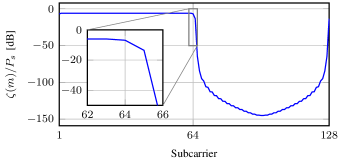
Figure 4: $\zeta(m)=\operatorname{\mathbb{R}e}\operatorname{tr}\Bigl{[}\mathbf{U}^{-}\mathcal{F}_{k}(m)\mathcal{X}^{\mathcal{R}-\frac{1}{2}\mathbb{I}}_{(p,q,p,q)}+\mathbf{U}^{+}\mathcal{F}_{k}(m)\mathcal{X}^{\mathcal{S}}_{(p,q,p,q)}\Bigr{]}$ for a user transmitting on subcarriers 1 to 64 with power $P_{s}$. The prototype pulse of Fig. 3 is employed at both the transmitter and the receiver side.

The behavior of $\zeta(m)$ is closely related to the frequency response of the prototype pulses employed in the FBMC system. To see this, consider the case where the overlapping factor is set to $\kappa=1$ (all other constraints, namely AS1, AS2, PR and symmetry, still hold). Also, let $p_{N}[n]=q_{N}[n]$, that is the same pulse is used on both sides. Then, matrix $\mathcal{R}(p_{N},q_{N})$ in (1) is actually a vector, namely

$$\mathcal{R}(p_{2M},p_{2M})=\mathbf{r}=\begin{bmatrix}p_{2M}^{2}[1]&\cdots&p_{2M}^{2}[2M]\end{bmatrix}^{T}.$$

Denote by $\boldsymbol{\rho}=[\rho_{1}\,\cdots\,\rho_{2M}]^{T}$ the DFT of $\mathbf{r}$, that is $\boldsymbol{\rho}=\mathbf{F}_{2M}^{H}\mathbf{r}$. Simple algebra allows us to rewrite the first term of $\zeta(m)$ as

$$\operatorname{\mathbb{R}e}\operatorname{tr}\Bigl{[}\mathbf{U}^{-}\mathcal{F}_{k}(m)\mathcal{X}^{\mathcal{R}-\frac{1}{2}\mathbb{I}}_{(p,q,p,q)}\Bigr{]}=2\sum_{n=1}^{M}|\rho_{2n}|^{2}\beta_{k,2n-m+1}$$ (14)

where $\beta_{k,n}=\operatorname{\mathbb{E}}[b_{k,n}^{2}]/(2M)$. For well designed prototype pulses, we will now prove that the right-hand side of (14) is identically null for most $m\notin\mathcal{I}_{k}$. Indeed, without loss of generality, we can assume that $\mathcal{I}_{k}=\{m_{\min},\dots,m_{\max}\}$ and, thus, $\beta_{k,n}\neq 0\Leftrightarrow m_{\min}\leq n\leq m_{\max}$. On the other hand, if the prototype pulses are low-pass filters, the number of nonzero Fourier coefficients is limited. More specifically, there exists an integer value $m_{0}$ (typically $m_{0}\approx 2\kappa$, see, e.g., [24]) such that $\rho_{n}\neq 0$ if and only if $1\leq n\leq m_{0}+1$ or $2M-m_{0}+1\leq n\leq 2M$ (recall that, since $\mathbf{r}$ is real, $\rho_{n}=\rho_{2M-n+2}$ for $n=2,\dots,2M$). Then, a careful inspection of the indices (Fig. 5 may help in this purpose) shows that $\zeta(m)$ is not zero if and only if $m_{\min}-m_{0}\leq m\leq m_{\max}+m_{0}$. Similar reasoning holds for the second term of $\zeta(m)$ and for all the other distortion terms $\eta_{x,y}(m)$. Conversely, by a similar reasoning, it is readily seen that the distortion terms $\eta_{x,y}(m)$ may be significantly different than zero for most $m$ if the spectrum containment property of the prototype pulses is not as strict and the number of nonzero Fourier coefficients is high. In this category we find pulses for time-limited orthogonal multicarrier modulation schemes [25] and some pulses maximizing the time–frequency localization of the signal [16, 7, 17, 18].

Figure 5: Circular cross-correlation of two vectors with few nonzero entries. Recall that $-m_{0}\equiv 2M-m_{0}$ modulo $2M$.

Summarizing the above discussion, an accurate design of the prototype pulses permits the out-band distortion to be confined within few subbands at the boundaries of the user of interest. A proper equalization (e.g. zero forcing), conversely, reduces the in-band distortion, since terms $\eta_{0,0}(m)$, $\eta_{0,1}(m)$ and $\eta_{0,2}(m)$ can be easily canceled out. Unfortunately, with the considered single-tap-per-subcarrier equalizer, no degrees of freedom are left to further minimize $\eta_{1,1}(m)$, which depends on the first derivative of the channel frequency response.

IV Numerical Analysis

In this section, the theoretical results above are verified against numerical ones obtained by simulating a realistic FBMC-based OFDMA channel. More specifically, we consider a scenario with $2M=128$ subcarriers, spaced by 15 kHz. The resulting total bandwidth of 1.920 MHz is thus compliant with the LTE standard [2]. The overlapping factor is set to $\kappa=4$ and the prototype pulse proposed by the EU-funded project PHYDYAS [23], depicted in Fig. 3, is used at both the transmitter side and the receiver side. Note that this pulse is not PR-compliant and, thus, the full distortion expression of Appendix A shall be used. We also assume that two users are accessing the channel and that each of them is assigned 64 subcarriers (subcarrier 1 to 64 to User 1 and subcarrier 65 to 128 to User 2). The equalizer is tuned according to the zero-forcing principle on each user’s subband, i.e. $W_{m}=H_{k}^{-1}(\omega_{m})$ for all $m\in\mathcal{I}_{k}$. All subcarriers are subject to a white Gaussian noise process with variance $\sigma^{2}$. Finally, the transmitted symbols are uniformly drawn from a 4QAM constellation with power $P_{s}$.

IV-A Theory Assessment

In order to test the above results with different degrees of channel frequency selectivity, we assume that the channels of the two users follow either the ITU Extended Pedestrian A (EPA) model or the ITU Extended Vehicular A (EVA) model [26]. More specifically, for the channel instances depicted in Fig. 6 and Fig. 7, we compute the subcarrier Signal-to-Noise-and-Distortion Ratio (SNDR) according to

$$\mathit{SNDR}(m)=\frac{P_{s}}{P_{e}(m)+P_{w}(m)}$$

where $P_{e}(m)=\sum_{k=1}^{2}P_{e,k}(m)$ is the total distortion, sum of users’ contributions as in (10), and $P_{w}(m)=\sigma^{2}{|W_{m}|}^{2}M^{-1}\sum_{n=1}^{N}q_{N}^{2}[n]$ is the noise power at the output of the filterbank. For both channel cases and for a Signal-to-Noise Ratio ($\mathit{SNR}=P_{s}/\sigma^{2}$) of either 20 dB or 40 dB, the results are depicted in Fig. 8 and compared to the empirical values obtained by averaging over 2000 multicarrier symbols. As one can observe, the two curves match perfectly.

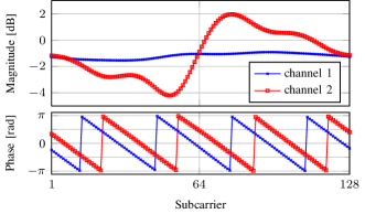
Figure 6: Two example realizations of EPA channel.

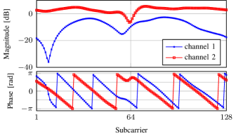
Figure 7: Two example realizations of EVA channel.

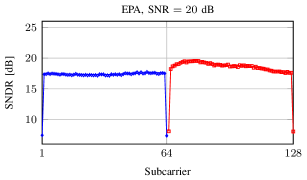
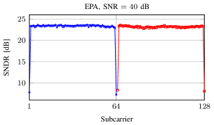
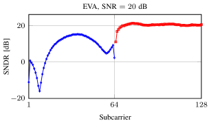
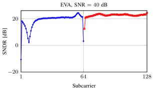
Figure 8: Theoretical (line) and empirical (markers) SNDR for the two-user case. The ratio $P_{s}/\sigma^{2}$ is set to 20 dB (left) and 40 dB (right). Reported examples correspond to EPA channel model (top) and EVA channel model (bottom).

It is interesting to note that, when increasing the transmit power from 20 dB to 40 dB over the noise level, the SNDR improves by a mere 6 dB and saturates at around 23 dB. This is indeed the inverse of the distortion level $P_{e}(m)/P_{s}$, as one can appreciate from Fig. 9. The curves of Fig. 9 also confirm that the in-band distortion (the one generated by a user in its own subband) is the main cause of signal degradation at high SNR. The out-band distortion, on the other hand, is significant only in the first subcarrier outside the user’s subband, as evinced from the peaks in Fig. 9 (and from the dips in Fig. 8). This could be predicted according to Section III-B1, keeping in mind that the Fourier coefficients of the prototype pulse in use are those reported in Table I (only $M$ coefficients are needed since the pulse is real-valued).

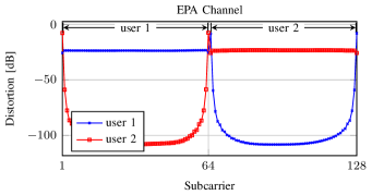
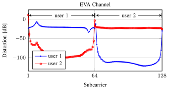
Figure 9: Normalized distortion power for the two users. Example of EPA channel model (top) and of EVA channel model (bottom).

TABLE I: Pulse Fourier Coefficients

Index	1	2	3	4	5–256
Magnitude	4.000	3.888	2.828	0.940	0

IV-B Delay Channels

In order to confirm the interest for FBMC/OQAM as an enabler technology for OFDMA, we compare the performances of the considered scheme with those of CP-OFDMA in a simple study case: the channels of both users do not introduce other impairment than a delay. More specifically, we consider the receiver to be perfectly synchronized with User 1, while User 2 is received with a delay equal to an integer number of samples. In what follows, we focus on how the delay of User 2 affects the SNDR of User 1. Note that, analogously, we could have focused on User 2. Indeed, even though the two users cannot synchronize to one another, it is realistic to assume that the BS is able to synchronize alternatively to both of them in order to retrieve their transmitted signal. The ability of FBMC to deal with the timing of each subcarrier (and hence of each user) separately is a strong advantage of this multicarrier multiple-access scheme when compared to classical CP-OFDM.

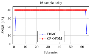
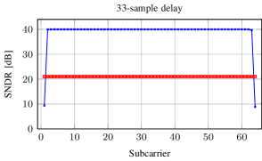
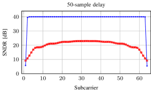
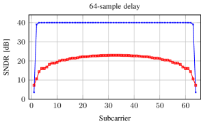
Figure 10: Comparison between FBMC-based OFDMA and CP-OFDMA: SNDR of User 1 for different delay values of User 2. The transmit SNR is set to 40 dB.

Fig. 10 shows the SNDR corresponding to the subcarriers of User 1 for different delays between the two users. The transmission scheme is either the FBMC/OQAM-based one described in the previous sections or a classic CP-OFDMA scheme with a cyclic prefix of 32 samples (25% of the number of subcarriers). Both users are assumed to transmit with a power that is 40 dB above the noise level. When the delay is shorter than the CP, CP-OFDMA is capable of compensating it perfectly and no distortion is introduced (see Fig. 10a corresponding to a delay of 16 samples). However, as soon as the delay between the two users is larger than the CP (see graphs b, c and d of Fig. 10) the performances of CP-OFDMA decay catastrophically, with a drop of 20 dB. A detailed analysis of the distortion generated in a CP-OFDMA system is reported in Appendix B.

Conversely, FBMC-based OFDMA proves itself robust to user asynchronicities: User 1 is received with the same SNDR in all the considered examples. More specifically, for all delay values, the quality of the received signal is approximately the same as the one obtained by CP-OFDMA in the short delay case (see Fig. 10a). Only the first and the last subcarriers show a significant degradation, due to the leakage effect discussed before.

IV-C Symbol Error Rate

To conclude our study and the comparison between the two multiple-access techniques, Fig. 11 reports some Symbol-Error-Rate (SER) curves obtained simulating the transmission of 1000 bursts of 100 multicarrier symbols. For each burst, the users’ channels are drawn independently according to the EVA model. SER is reported as a function of the received energy per bit $E_{b}$, normalized with respect to the noise spectral density $N_{0}$. A single guard band separates the users (subcarriers 64 and 128 are switched off).

Two different synchronization assumptions are considered. In the first one (top graphs), the transmissions of the two users are synchronized. In this case, CP-OFDMA follows the theoretic performance of the chosen QAM constellation (4QAM for the left graphs and 16QAM for the right ones [27, Chapter 5]) with a 1-dB loss, approximately, due to the CP overhead. Indeed, the length of the channel (around 14 taps for the EVA model with a 1.92-MHz bandwidth) is perfectly compensated by the 32-sample CP. Conversely, FBMC is closer to the theoretic curve at low $E_{b}/N_{0}$ values, but its performance worsens as we increase the SNR due to the inherent interference discussed above, as suggested by the curve floor visible in the 16QAM case. (In the 4QAM case, the SER floor of the FBMC curve falls outside the depicted range.)

The bottom graphs, on the other hand, are obtained introducing a delay between the two users. This delay is equal to an integer number of samples, varies at each burst and is uniformly distributed between 0 and 127 samples (i.e. one multicarrier symbol). As we can see from Fig. 11, asynchronous transmissions do not imply a significant performance loss for the FBMC configuration. This is not the case for the scheme based on CP-OFDM: since the CP is too short to compensate the total length of the channel (delay plus impulse response), the SER does not improve as desired for $E_{b}/N_{0}>10$ dB and the performance is much worse than for the FBMC scheme.

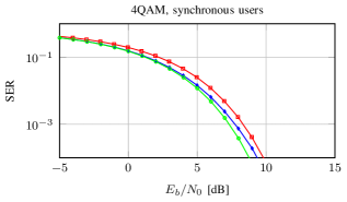
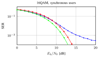
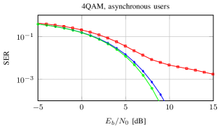
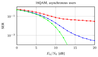
Figure 11: Symbol error rate as a function of $E_{b}/N_{0}$ (measured at the receiver side) for FBMC-based OFDMA and CP-OFDMA. Users’ transmissions are either synchronized (top) or not (bottom) and the transmitted symbols belong either to a 4QAM constellation (left) or to a 16QAM constellation (right).

It is worth remarking that the FBMC curves are obtained with a suboptimal one-tap per-subcarrier equalizer. The performance gap between FBMC-based OFDMA and CP-OFDMA will increase by employing receiver structures such as [8, 11], which will lower the FBMC error floor. Even if the equalizers described in [8, 11] are more complex than a CP-OFDM one-tap per-subcarrier equalizer, they are still a competitive solution when compared with hardware and protocol requirements of classic OFDMA with short CP [3].

V Conclusions

In this paper we have rigorously analyzed the interaction between users in an FBMC/OQAM-based OFDMA system. More specifically, for a reasonably high number of subcarriers, we have been able to express the per-subcarrier interference as the sum of users’ terms. It is important to remark that, in general, the distortion at a given subcarrier does not depend exclusively on the user transmitting on that subcarrier, but also on all other users. Our analysis shows that, when the prototype pulses are well designed, the distortion caused by a given user decays steeply outside the user’s subband and can be neglected after few subcarriers (or even after a single subcarrier, as in the example of Fig. 9). This result supports the choice of placing a single empty guard band between users. To the best of our knowledge, such a choice was only empirically justified until now. Moreover, the spread of the out-band interference depends neither on the channel responses (of any user) nor on the equalizer coefficients, thus simplifying the task of designing the prototype pulses.

As for the comparison to the more classical CP-OFDMA scheme, the ideal case with synchronized users suggests that the FBMC approach is not worth the complexity. Indeed, the CP causes a loss in the order of 1 dB at low-to-medium SNR, but avoids performance floors at high SNR (see Fig. 11, top graphs). However, in more practical scenarios where users’ transmissions are not synchronized, the length of the equivalent channel (delay plus impulse response) can easily exceed the CP. In this situation, the performance of CP-OFDMA drops abruptly, whereas the FBMC scheme proves to be very robust, showing no significant degradation and without need for any extra signal processing (see Fig. 11, bottom graphs).

Summarizing, filterbank modulations offer a convenient solution to the multiple-access channel problem, since they can deal with asynchronous users without increasing complexity. Furthermore, the tools presented in this paper allow the designer to choose the prototype pulses that minimize both inter-user interference and number of guard bands. Remarkably, no channel state information is needed to carry out this task.

Appendix A Proof of Proposition 1

In this appendix we show how the terms in (11) are derived. To do so, we first obtain a general expression for the distortion generated by user $k$ at subcarrier $m$. Then, the simplified form in (11) is obtained by particularizing to the the special case considered in Proposition 1.

A-A The General Case

For practical reasons, let us define the following matrices and vectors:

$$\mathbf{y}_{k}^{\text{odd}}\Bigl{(}p_{N},q_{N}^{(r)}\Bigr{)} ={\Bigl{[}\mathbf{Y}_{k}^{\text{odd}}\Bigl{(}p_{N},q_{N}^{(r)}\Bigr{)}\Bigr{]}}_{:,n+\kappa-1}$$

$$\overline{\mathbf{y}_{k}^{\text{odd}}}\Bigl{(}p_{N},q_{N}^{(r)}\Bigr{)} =\begin{bmatrix}\operatorname{\mathbb{R}e}\Bigl{\{}\mathbf{y}_{k}^{\text{odd}}\Bigl{(}p_{N},q_{N}^{(r)}\Bigr{)}\Bigr{\}}\\ -\operatorname{\mathbb{I}m}\Bigl{\{}\mathbf{y}_{k}^{\text{odd}}\Bigl{(}p_{N},q_{N}^{(r)}\Bigr{)}\Bigr{\}}\end{bmatrix}$$

$$t_{k,m}(i) =\frac{(-\mathrm{j})^{i}}{i!}W_{m}H_{k}^{(i)}(\omega_{m}),\hskip 20.00003pti=0,1,2$$

$$\mathbf{T}_{k}(i) =\operatorname{diag}_{m=1,\dots,2M}{\{t_{k,m}(i)\}}$$

$$=\frac{(-\mathrm{j})^{i}}{i!}\mathbf{W}\boldsymbol{\Lambda}_{H_{k}^{(i)}},\hskip 20.00003pti=0,1,2$$

$$\mathbf{t}_{k,m}(i) =\begin{bmatrix}\mathbf{0}_{m-1}\\ \operatorname{\mathbb{R}e}\{t_{k,m}(i)\}\\ \mathbf{0}_{2M}\\ \operatorname{\mathbb{I}m}\{t_{k,m}(i)\}\\ \mathbf{0}_{2M-m-1}\end{bmatrix}$$ (15)

and, for a generic column vector $$\mathbf{u}\in\mathbb{C}^{2M}$$,

$$\mathcal{M}(\mathbf{u}) =\mathbf{\Phi}\mathbf{F}_{2M}^{H}\operatorname{diag}\bigl{\{}\mathbf{F}_{2M}\mathbf{\Phi}^{*}\mathbf{u}\bigr{\}}$$

$$\widetilde{\mathcal{M}}(\mathbf{u}) =\mathbf{\Phi}\mathbf{F}_{2M}^{H}\operatorname{diag}\bigl{\{}(\mathbf{J}_{2}\otimes\mathbf{I}_{M})\mathbf{F}_{2M}\mathbf{\Phi}^{*}\mathbf{u}\bigr{\}}.$$

Then, denoting by $\mathbf{b}_{k}(r)$ [$\mathbf{c}_{k}(r)$, respectively] the $r$-th column of $\mathbf{B}_{k}$ ($\mathbf{C}_{k}$, respectively), from (3) one can write

$$\mathbf{y}_{k}^{\text{odd}}\Bigl{(}p_{N},q_{N}^{(r)}\Bigr{)}=2\sum_{i=1}^{N_{s}}\mathcal{M}\bigl{(}\mathbf{b}_{k}(i)\bigr{)}{[\mathcal{R}(p_{N},q_{N}^{(r)})]}_{:,n+\kappa-i}\\ {}+2\sum_{i=1}^{N_{s}}\widetilde{\mathcal{M}}\bigl{(}\mathrm{j}\mathbf{c}_{k}(i)\bigr{)}\begin{bmatrix}{[\mathcal{S}_{1}(p_{N},q_{N}^{(r)}]}_{:,n+\kappa-1-i}\\ {[\mathcal{S}_{2}(p_{N},q_{N}^{(r)}]}_{:,n+\kappa-i}\end{bmatrix}$$ (16)

where all column vectors are intended identically null when the column index is negative or higher than $2\kappa-1$. Moreover, keeping (7) and (15) in mind, the distortion can be expressed as follows:

$$\operatorname{\mathbb{E}}\biggl{[}{\Bigl{|}\operatorname{\mathbb{R}e}[z_{k,m}^{\text{odd}}]-t_{k,m}(0)b_{k,m}\Bigr{|}}^{2}\biggr{]}=\eta_{0,0}(m)+\frac{2}{2M}\eta_{0,1}(m)\\ {}+\frac{1}{4M^{2}}\eta_{0,2}(m)+\frac{1}{4M^{2}}\eta_{1,1}(m)+o\bigl{(}M^{-2}\bigr{)}$$

where

$$\eta_{0,0}(m)=\> \mathbf{t}_{k,m}^{T}(0)\operatorname{\mathbb{E}}\biggl{[}\Bigl{(}\overline{\mathbf{y}^{\text{odd}}_{k}}(p_{N},q_{N})-{[\mathbf{b}_{k}^{T}(n),\mathbf{0}_{2M}^{T}]}^{T}\Bigr{)}\Bigl{(}\overline{\mathbf{y}^{\text{odd}}_{k}}(p_{N},q_{N})-{[\mathbf{b}_{k}^{T}(n),\mathbf{0}_{2M}^{T}]}^{T}\Bigr{)}^{T}\biggr{]}\mathbf{t}_{k,m}(0)$$

$$\eta_{0,1}(m)=\> \mathbf{t}_{k,m}^{T}(0)\operatorname{\mathbb{E}}\biggl{[}\Bigl{(}\overline{\mathbf{y}^{\text{odd}}_{k}}(p_{N},q_{N})-{[\mathbf{b}_{k}^{T}(n),\mathbf{0}_{2M}^{T}]}^{T}\Bigr{)}\times\Bigl{(}\overline{\mathbf{y}^{\text{odd}}_{k}}(p_{N},q_{N}^{\prime})\Bigr{)}^{T}\biggr{]}\mathbf{t}_{k,m}(1)$$

$$\eta_{0,2}(m)=\> \mathbf{t}_{k,m}^{T}(0)\operatorname{\mathbb{E}}\biggl{[}\Bigl{(}\overline{\mathbf{y}^{\text{odd}}_{k}}(p_{N},q_{N})-{[\mathbf{b}_{k}^{T}(n),\mathbf{0}_{2M}^{T}]}^{T}\Bigr{)}\Bigl{(}\overline{\mathbf{y}^{\text{odd}}_{k}}(p_{N},q_{N}^{\prime\prime})\Bigr{)}^{T}\biggr{]}\mathbf{t}_{k,m}(2)$$

$$\eta_{1,1}(m)=\> \mathbf{t}_{k,m}^{T}(1)\operatorname{\mathbb{E}}\biggl{[}\Bigl{(}\overline{\mathbf{y}^{\text{odd}}_{k}}(p_{N},q_{N}^{\prime})\Bigr{)}\Bigl{(}\overline{\mathbf{y}^{\text{odd}}_{k}}(p_{N},q_{N}^{\prime})\Bigr{)}^{T}\biggr{]}\mathbf{t}_{k,m}(1).$$

Before taking the next step, we need to introduce the following result, whose proof follows the same lines as [11, Lemma 2].

$$\eta_{0,0}(m)=\> 2\operatorname{\mathbb{R}e}^{2}[t_{k,m}(0)]\operatorname{\mathbb{R}e}\operatorname{tr}\Bigl{[}\mathbf{U}^{+}\mathcal{F}_{k}(m)\mathcal{X}^{\mathcal{R}-\frac{1}{2}\mathbb{I}}_{(p,q,p,q)}+\mathbf{U}^{-}\mathcal{F}_{k}(m)\mathcal{X}^{\mathcal{S}}_{(p,q,p,q)}\Bigr{]}$$

$${}+2\operatorname{\mathbb{I}m}^{2}[t_{k,m}(0)]\operatorname{\mathbb{R}e}\operatorname{tr}\Bigl{[}\mathbf{U}^{-}\mathcal{F}_{k}(m)\mathcal{X}^{\mathcal{R}-\frac{1}{2}\mathbb{I}}_{(p,q,p,q)}+\mathbf{U}^{+}\mathcal{F}_{k}(m)\mathcal{X}^{\mathcal{S}}_{(p,q,p,q)}\Bigr{]}$$

$${}-4\operatorname{\mathbb{R}e}[t_{k,m}(0)]\operatorname{\mathbb{I}m}[t_{k,m}(0)]$$

$$\qquad{}\times\operatorname{\mathbb{I}m}\operatorname{tr}\Bigl{[}(\mathbf{I}_{2}\otimes\mathbf{J}_{M})\mathcal{F}_{k}(m)\mathcal{X}^{\mathcal{R}-\frac{1}{2}\mathbb{I}}_{(p,q,p,q)}-(\mathbf{I}_{2}\otimes\mathbf{J}_{M})\mathcal{F}_{k}(m)\mathcal{X}^{\mathcal{S}}_{(p,q,p,q)}\Bigr{]}$$ (17a)

$$\eta_{0,1}(m)=\> 2\operatorname{\mathbb{R}e}[t_{k,m}(0)]\operatorname{\mathbb{R}e}[t_{k,m}(1)]\operatorname{\mathbb{R}e}\operatorname{tr}\Bigl{[}\mathbf{U}^{+}\mathcal{F}_{k}(m)\mathcal{X}^{\mathcal{R}-\frac{1}{2}\mathbb{I},\mathcal{R}}_{(p,q,p,q^{\prime})}+\mathbf{U}^{-}\mathcal{F}_{k}(m)\mathcal{X}^{\mathcal{S}}_{(p,q,p,q^{\prime})}\Bigr{]}$$

$${}+2\operatorname{\mathbb{I}m}[t_{k,m}(0)]\operatorname{\mathbb{I}m}[t_{k,m}(1)]\operatorname{\mathbb{R}e}\operatorname{tr}\Bigl{[}\mathbf{U}^{-}\mathcal{F}_{k}(m)\mathcal{X}^{\mathcal{R}-\frac{1}{2}\mathbb{I},\mathcal{R}}_{(p,q,p,q^{\prime})}+\mathbf{U}^{+}\mathcal{F}_{k}(m)\mathcal{X}^{\mathcal{S}}_{(p,q,p,q^{\prime})}\Bigr{]}$$

$${}+2\operatorname{\mathbb{R}e}[t_{k,m}(0)]\operatorname{\mathbb{I}m}[t_{k,m}(1)]\operatorname{\mathbb{I}m}\operatorname{tr}\Bigl{[}\mathbf{U}^{-}\mathcal{F}_{k}(m)\mathcal{X}^{\mathcal{R}-\frac{1}{2}\mathbb{I},\mathcal{R}}_{(p,q,p,q^{\prime})}+\mathbf{U}^{+}\mathcal{F}_{k}(m)\mathcal{X}^{\mathcal{S}}_{(p,q,p,q^{\prime})}\Bigr{]}$$

$${}-2\operatorname{\mathbb{I}m}[t_{k,m}(0)]\operatorname{\mathbb{R}e}[t_{k,m}(1)]\operatorname{\mathbb{I}m}\operatorname{tr}\Bigl{[}\mathbf{U}^{+}\mathcal{F}_{k}(m)\mathcal{X}^{\mathcal{R}-\frac{1}{2}\mathbb{I},\mathcal{R}}_{(p,q,p,q^{\prime})}+\mathbf{U}^{-}\mathcal{F}_{k}(m)\mathcal{X}^{\mathcal{S}}_{(p,q,p,q^{\prime})}\Bigr{]}$$ (17b)

$$\eta_{0,2}(m)=\> 2\operatorname{\mathbb{R}e}[t_{k,m}(0)]\operatorname{\mathbb{R}e}[t_{k,m}(2)]\operatorname{\mathbb{R}e}\operatorname{tr}\Bigl{[}\mathbf{U}^{+}\mathcal{F}_{k}(m)\mathcal{X}^{\mathcal{R}-\frac{1}{2}\mathbb{I},\mathcal{R}}_{(p,q,p,q^{\prime\prime})}+\mathbf{U}^{-}\mathcal{F}_{k}(m)\mathcal{X}^{\mathcal{S}}_{(p,q,p,q^{\prime\prime})}\Bigr{]}$$

$${}+2\operatorname{\mathbb{I}m}[t_{k,m}(0)]\operatorname{\mathbb{I}m}[t_{k,m}(2)]\operatorname{\mathbb{R}e}\operatorname{tr}\Bigl{[}\mathbf{U}^{-}\mathcal{F}_{k}(m)\mathcal{X}^{\mathcal{R}-\frac{1}{2}\mathbb{I},\mathcal{R}}_{(p,q,p,q^{\prime\prime})}+\mathbf{U}^{+}\mathcal{F}_{k}(m)\mathcal{X}^{\mathcal{S}}_{(p,q,p,q^{\prime\prime})}\Bigr{]}$$

$${}+2\operatorname{\mathbb{R}e}[t_{k,m}(0)]\operatorname{\mathbb{I}m}[t_{k,m}(2)]\operatorname{\mathbb{I}m}\operatorname{tr}\Bigl{[}\mathbf{U}^{-}\mathcal{F}_{k}(m)\mathcal{X}^{\mathcal{R}-\frac{1}{2}\mathbb{I},\mathcal{R}}_{(p,q,p,q^{\prime\prime})}+\mathbf{U}^{+}\mathcal{F}_{k}(m)\mathcal{X}^{\mathcal{S}}_{(p,q,p,q^{\prime\prime})}\Bigr{]}$$

$${}-2\operatorname{\mathbb{I}m}[t_{k,m}(0)]\operatorname{\mathbb{R}e}[t_{k,m}(2)]\operatorname{\mathbb{I}m}\operatorname{tr}\Bigl{[}\mathbf{U}^{+}\mathcal{F}_{k}(m)\mathcal{X}^{\mathcal{R}-\frac{1}{2}\mathbb{I},\mathcal{R}}_{(p,q,p,q^{\prime\prime})}+\mathbf{U}^{-}\mathcal{F}_{k}(m)\mathcal{X}^{\mathcal{S}}_{(p,q,p,q^{\prime\prime})}\Bigr{]}$$ (17c)

$$\eta_{1,1}(m)=\> 2\operatorname{\mathbb{R}e}^{2}[t_{k,m}(1)]\operatorname{\mathbb{R}e}\operatorname{tr}\Bigl{[}\mathbf{U}^{+}\mathcal{F}_{k}(m)\mathcal{X}^{\mathcal{R}}_{(p,q^{\prime},p,q^{\prime})}+\mathbf{U}^{-}\mathcal{F}_{k}(m)\mathcal{X}^{\mathcal{S}}_{(p,q^{\prime},p,q^{\prime})}\Bigr{]}$$

$${}+2\operatorname{\mathbb{I}m}^{2}[t_{k,m}(1)]\operatorname{\mathbb{R}e}\operatorname{tr}\Bigl{[}\mathbf{U}^{-}\mathcal{F}_{k}(m)\mathcal{X}^{\mathcal{R}}_{(p,q^{\prime},p,q^{\prime})}+\mathbf{U}^{+}\mathcal{F}_{k}(m)\mathcal{X}^{\mathcal{S}}_{(p,q^{\prime},p,q^{\prime})}\Bigr{]}$$

$${}-4\operatorname{\mathbb{R}e}[t_{k,m}(1)]\operatorname{\mathbb{I}m}[t_{k,m}(1)]$$

$$\qquad{}\times\operatorname{\mathbb{I}m}\operatorname{tr}\Bigl{[}(\mathbf{I}_{2}\otimes\mathbf{J}_{M})\mathcal{F}_{k}(m)\mathcal{X}^{\mathcal{R}}_{(p,q^{\prime},p,q^{\prime})}-(\mathbf{I}_{2}\otimes\mathbf{J}_{M})\mathcal{F}_{k}(m)\mathcal{X}^{\mathcal{S}}_{(p,q^{\prime},p,q^{\prime})}\Bigr{]}$$ (17d)

 

Lemma 1

Let $\mathbf{u}\in\mathbb{R}^{2M}$ be a real-valued random vector of independent entries with zero mean and diagonal covariance matrix $\mathbf{Q}_{u}$. Recalling the definitions of $\mathbf{U}^{+}$ and $\mathbf{U}^{-}$ in (6), and for $m=1,\dots,2M$, we can write

$$\operatorname{\mathbb{E}}\biggl{[}{\bigl{[}\mathcal{M}^{\operatorname{\mathbb{R}e}}(\mathbf{u})\bigr{]}}_{m,:}^{T}{\bigl{[}\mathcal{M}^{\operatorname{\mathbb{R}e}}(\mathbf{u})\bigr{]}}_{m,:}\biggr{]} =\frac{1}{2}\mathbf{U}^{+}\operatorname{\mathbb{R}e}\{\mathcal{F}_{u}(m)\}$$

$$\operatorname{\mathbb{E}}\biggl{[}{\bigl{[}\mathcal{M}^{\operatorname{\mathbb{I}m}}(\mathbf{u})\bigr{]}}_{m,:}^{T}{\bigl{[}\mathcal{M}^{\operatorname{\mathbb{I}m}}(\mathbf{u})\bigr{]}}_{m,:}\biggr{]} =\frac{1}{2}\mathbf{U}^{-}\operatorname{\mathbb{R}e}\{\mathcal{F}_{u}(m)\}$$

$$\operatorname{\mathbb{E}}\biggl{[}{\bigl{[}\mathcal{M}^{\operatorname{\mathbb{R}e}}(\mathbf{u})\bigr{]}}_{m,:}^{T}{\bigl{[}\mathcal{M}^{\operatorname{\mathbb{I}m}}(\mathbf{u})\bigr{]}}_{m,:}\biggr{]} =\frac{1}{2}\mathbf{U}^{+}\operatorname{\mathbb{I}m}\{\mathcal{F}_{u}(m)\}$$

$$\operatorname{\mathbb{E}}\biggl{[}{\bigl{[}\mathcal{M}^{\operatorname{\mathbb{I}m}}(\mathbf{u})\bigr{]}}_{m,:}^{T}{\bigl{[}\mathcal{M}^{\operatorname{\mathbb{R}e}}(\mathbf{u})\bigr{]}}_{m,:}\biggr{]} =-\frac{1}{2}\mathbf{U}^{-}\operatorname{\mathbb{I}m}\{\mathcal{F}_{u}(m)\}$$

where $\mathcal{F}_{u}(m)=\mathbf{F}_{2M}^{H}\mathbf{Q}_{u}\mathbf{F}_{2M}\odot\mathbf{f}(m)\mathbf{f}^{H}(m)$, together with $\mathcal{M}^{\operatorname{\mathbb{R}e}}(\mathbf{u})=\operatorname{\mathbb{R}e}\{\mathcal{M}(\mathbf{u})\}$ and $\mathcal{M}^{\operatorname{\mathbb{I}m}}(\mathbf{u})=\operatorname{\mathbb{I}m}\{\mathcal{M}(\mathbf{u})\}$.

The same results hold when $\mathcal{M}(\mathbf{u})$ is replaced everywhere by $\widetilde{\mathcal{M}}(\mathbf{u})$.

Given (16), a direct application of this lemma to $\eta_{1,1}(m)$ yields (17d) at the top of the page. Recall that $\mathcal{X}^{\mathcal{R}}_{(p,q^{\prime},p,q^{\prime})}$ and $\mathcal{X}^{\mathcal{S}}_{(p,q^{\prime},p,q^{\prime})}$ are defined in (12) and (13), respectively, and that $\mathcal{F}_{k}(m)=\mathbf{F}_{2M}^{H}\mathbf{Q}_{k}\mathbf{F}_{2M}\odot\mathbf{f}(m)\mathbf{f}^{H}(m)$, with $\mathbf{Q}_{k}=\operatorname{\mathbb{E}}[\mathbf{b}_{k}(r)\mathbf{b}_{k}^{T}(r)]=\operatorname{\mathbb{E}}[\mathbf{c}_{k}(r)\mathbf{c}_{k}^{T}(r)]$, for any $r=1,\dots,N_{s}$.

Similar expressions can be found for the other three terms $\eta_{0,0}(m)$, $\eta_{0,1}(m)$ and $\eta_{0,2}(m)$, also [see (17a)–(17c)]. Indeed, it is enough to realize that (16) holds true even if we replace $\mathbf{y}_{k}^{\text{odd}}(p_{N},q_{N})$ by $\mathbf{y}_{k}^{\text{odd}}(p_{N},q_{N})-\mathbf{b}_{k}(n)$ and $\mathcal{R}(p_{N},q_{N})$ by $\mathcal{R}(p_{N},q_{N})-\frac{1}{2}\mathbb{I}$.

A-B The Special Case of Proposition 1

In the previous section we have derived a general expression for the distortion caused by user $k$ at subcarrier $m$ and shown how it depends on 1. the power/resource allocation policy through matrix $\mathcal{F}_{k}(m)$, 2. the channel and the chosen equalizer through coefficients $t_{k,m}(i)$, and 3. the prototype pulses through matrices $\mathcal{R}(p_{N},q_{N}^{(r)})$ and $\mathcal{S}(p_{N},q_{N}^{(r)})$. It is worth remarking that the expression is as general as possible and holds for any choice of prototype pulses $p_{N}[n]$ and $q_{N}[n]$ that fulfill assumptions AS1 and AS2. More specifically, there are no requirements about symmetry or perfect reconstruction. In what follows, we show how the distortion terms simplify to (11) when the prototype pulses are symmetric (e.g. $p_{N}[n]=p_{N}[N-n+1]$) and meet PR conditions (5).

To that purpose, we need the two following results. Proofs are omitted to due to space constraints, but are straightforward consequences of the fact that $\mathcal{F}_{k}(m)$ is a circulant matrix.

Lemma 2

For any $2M\times 2M$ complex matrix $\mathbf{A}$ the following identities hold true (note the commuting signs in the second equation):

$$\operatorname{\mathbb{R}e}\operatorname{tr}\Bigl{[}\mathbf{U}^{\pm}\mathcal{F}_{k}(m)\mathbf{A}\Bigr{]} =\frac{1}{2}\operatorname{\mathbb{R}e}\operatorname{tr}\Bigl{[}\mathcal{F}_{k}(m)\mathbf{U}^{\pm}\mathbf{A}\mathbf{U}^{\pm}\Bigr{]}$$

$$\operatorname{\mathbb{I}m}\operatorname{tr}\Bigl{[}\mathbf{U}^{\pm}\mathcal{F}_{k}(m)\mathbf{A}\Bigr{]} =\frac{1}{2}\operatorname{\mathbb{I}m}\operatorname{tr}\Bigl{[}\mathcal{F}_{k}(m)\mathbf{U}^{\mp}\mathbf{A}\mathbf{U}^{\pm}\Bigr{]}.$$

Lemma 3

Let $\mathbf{A}$ be a $2M\times 2M$ complex matrix such that

$$\mathbf{A}=\begin{bmatrix}\mathbf{A}_{1}&\mathbf{A}_{2}\\ -\mathbf{A}_{2}&-\mathbf{A}_{1}\end{bmatrix}.$$

Then

$$\operatorname{tr}\Bigl{[}\mathcal{F}_{k}(m)\mathbf{A}\Bigr{]}=0.$$

Lemma 2, together with (5), implies that most of the terms in (17) cancel out when the prototype pulses meet the PR conditions. Take, for instance, the first term of $\eta_{0,0}(m)$. We have

$$2\operatorname{\mathbb{R}e}\operatorname{tr}\Bigl{[}\mathbf{U}^{+}\mathcal{F}_{k}(m)\mathcal{X}^{\mathcal{R}-\frac{1}{2}\mathbb{I}}_{(p,q,p,q)}\Bigr{]}=\operatorname{\mathbb{R}e}\operatorname{tr}\Bigl{[}\mathcal{F}_{k}(m)\mathbf{U}^{+}\mathcal{X}^{\mathcal{R}-\frac{1}{2}\mathbb{I}}_{(p,q,p,q)}\mathbf{U}^{+}\Bigr{]}=0$$

where we have used the fact that (5a) can be rewritten as $\mathbf{U}^{+}\Bigl{(}\mathcal{R}(p_{N},q_{N})-\frac{1}{2}\mathbb{I}\Bigr{)}=\mathbf{0}$.

Assume now that the prototype pulses are also symmetric, besides PR-compliant. Note that if $q_{N}[n]$ is symmetric (i.e. $q_{N}[n]=q_{N}[N-n+1]$), then so is its second derivative (i.e. $q_{N}^{\prime\prime}[n]=q_{N}^{\prime\prime}[N-n+1]$), while the first derivative is anti-symmetric (i.e. $q_{N}^{\prime}[n]=-q_{N}^{\prime}[N-n+1]$). In this case, other terms null out as a consequence of Lemma 3. For example, for the second term of $\eta_{0,1}(m)$, we have

$$2\operatorname{\mathbb{R}e}\operatorname{tr}\Bigl{[}\mathbf{U}^{-}\mathcal{F}_{k}(m)\mathcal{X}^{\mathcal{R}-\frac{1}{2}\mathbb{I},\mathcal{R}}_{(p,q,p,q^{\prime})}\Bigr{]}=\operatorname{\mathbb{R}e}\operatorname{tr}\Bigl{[}\mathcal{F}_{k}(m)\mathbf{U}^{-}\mathcal{X}^{\mathcal{R}-\frac{1}{2}\mathbb{I},\mathcal{R}}_{(p,q,p,q^{\prime})}\mathbf{U}^{-}\Bigr{]}=\mathbf{0}$$

since the symmetry properties of $p_{N}[n]$ and $q_{N}[n]$, together with $\mathbf{U}^{-}\mathbb{I}=0$, imply that product matrix $\mathbf{U}^{-}\mathcal{X}^{\mathcal{R}-\frac{1}{2}\mathbb{I},\mathcal{R}}_{(p,q,p,q^{\prime})}\mathbf{U}^{-}$ meets the hypothesis of Lemma 3.

We have thus proven how the general distortion terms in (17) simplify into those of (11) when the prototype pulses are symmetric and satisfy the PR conditions.

A-C The Single-User Case

The distortion formula (10) with terms $\eta_{x,y}(m)$ given by (17) holds for all prototype pulses and for any number of users. In particular, for $K=1$, it allows computing the distortion of a single-user FBMC/OQAM link with a one-tap equalizer per subcarrier. The resulting expression

$$P_{e}(m)=\frac{P_{s}}{M}\operatorname{tr}\Bigl{[}\mathbf{U}^{+}\mathcal{X}^{\mathcal{R}-\frac{1}{2}\mathbb{I}}_{(p,q,p,q)}\Bigr{]}+\frac{P_{s}}{M^{2}}\operatorname{\mathbb{I}m}\Bigl{[}W_{m}H^{(1)}(\omega_{m})\Bigr{]}\operatorname{tr}\Bigl{[}\mathbf{U}^{+}\mathcal{X}^{\mathcal{R}-\frac{1}{2}\mathbb{I},\mathcal{R}}_{(p,q,p,q^{\prime})}\Bigr{]}\\ {}-\frac{P_{s}}{4M^{3}}\operatorname{\mathbb{R}e}\Bigl{[}W_{m}H^{(2)}(\omega_{m})\Bigr{]}\operatorname{tr}\Bigl{[}\mathbf{U}^{+}\mathcal{X}^{\mathcal{R}-\frac{1}{2}\mathbb{I},\mathcal{R}}_{(p,q,p,q")}\Bigr{]}\\ {}+\frac{P_{s}}{4M^{3}}{\Bigl{|}W_{m}H^{(1)}(\omega_{m})\Bigr{|}}^{2}\operatorname{tr}\biggl{[}\mathbf{U}^{+}\mathcal{X}^{\mathcal{R}}_{(p,q^{\prime},p,q^{\prime})}+\mathbf{U}^{-}\mathcal{X}^{\mathcal{S}}_{(p,q^{\prime},p,q^{\prime})}\biggr{]}$$ (18)

is thus a generalization of [11, Eq. (35)], which refers to the PR case.

Appendix B Distortion in CP-OFDM

This appendix derives an expression for the signal distortion in a CP-OFDMA system where the length of the channel is larger than the cyclic prefix. More specifically, we consider a CP of length $L$ and a channel of length $L+L_{T}$ with taps $\{h_{k,\ell}\}_{\ell=1,\dots,L+L_{T}}$ (for simplicity, we assume here that $L_{T}<L<2M$). The resulting distortion expression was used to draw the CP-OFDM curves in Fig. 10.

Maintaining the same notation as in Section II, the contribution to the output signal due to user $k$ can be written as

$$\mathbf{Z}_{k}^{\text{(CP)}}=\mathbf{W}\mathbf{F}_{2M}^{H}\overline{\mathbf{\Psi}}\mathbf{H}_{k}\mathbf{\Psi}\mathbf{F}_{2M}[\mathbf{A}_{k}\;\mathbf{0}]+\mathbf{W}\mathbf{F}_{2M}^{H}\overline{\mathbf{\Psi}}\mathbf{H}_{k,T}\mathbf{\Psi}\mathbf{F}_{2M}[\mathbf{0}\;\mathbf{A}_{k}]$$ (19)

where matrices

$$\mathbf{\Psi} =\begin{bmatrix}\mathbf{0}_{L\times(2M-L)}\;\mathbf{I}_{L}\\ \mathbf{I}_{2M}\end{bmatrix} \overline{\mathbf{\Psi}} =\begin{bmatrix}\mathbf{0}_{2M\times L}\;\mathbf{I}_{2M}\end{bmatrix}$$

apply and remove the CP of length $L$, respectively. The $(2M+L)\times(2M+L)$ channel matrix $\mathbf{H}_{k}$ is a lower triangular Toeplitz matrix whose first column is $[h_{k,1}\;\cdots\;h_{k,L+L_{T}}\;\mathbf{0}_{1\times(2M-L_{T})}]^{T}$. Similarly, the $(2M+L)\times(2M+L)$ matrix $\mathbf{H}_{k,T}$ is a upper triangular Toeplitz matrix whose first row is $[\mathbf{0}_{1\times(2M-L_{T}+1)}\;h_{k,L+L_{T}}\;\cdots\;h_{k,2}]$.

It is straightforward to realize that (19) corresponds to the classic OFDM model when $L_{T}=1$ and the CP covers the entire channel length. Indeed, $L_{T}=1$ implies $\mathbf{H}_{k,T}=\mathbf{0}$. Also, we have

$$\mathbf{\Lambda}_{H_{k}}=\mathbf{F}_{2M}^{H}\overline{\mathbf{\Psi}}\mathbf{H}_{k}\mathbf{\Psi}\mathbf{F}_{2M}$$

where $\mathbf{\Lambda}_{H_{k}}$ is the diagonal matrix filled with the channel frequency response defined in Section II. Thus, for channels not longer than $L+1$ taps, it is enough to set $\mathbf{W}=\mathbf{\Lambda}_{H_{k}}^{-1}$ to recover the transmitted symbols perfectly, namely $\mathbf{Z}_{k}^{\text{(CP)}}=[\mathbf{A}_{k}\;\mathbf{0}]$.

Conversely, when $L_{T}>1$, matrix $\overline{\mathbf{\Psi}}\mathbf{H}_{k}\mathbf{\Psi}$ is not diagonalizable anymore and an extra term appears. Namely

$$\overline{\mathbf{\Psi}}\mathbf{H}_{k}\mathbf{\Psi}=\mathbf{F}_{2M}\mathbf{\Lambda}_{H_{k}}\mathbf{F}_{2M}^{H}-\widetilde{\mathbf{H}}_{k}$$

where we introduced the $2M\times 2M$ matrix

$$\widetilde{\mathbf{H}}_{k}=\begin{bmatrix}\mathbf{0}_{(L_{T}-1)\times(2M-L-L_{T}+1)}&\mathbf{T}_{k}&\mathbf{0}_{(L_{T}-1)\times L}\\ &\makebox[15.00002pt][l]{$\mathbf{0}_{(2M-L_{T}+1)\times 2M}$}\end{bmatrix}$$ (20)

and where $\mathbf{T}_{k}$ is a $(L_{T}-1)\times(L_{T}-1)$ upper triangular Toeplitz matrix with $[h_{k,L+L_{T}}\;\cdots\;h_{k,L+2}]$ as its first row. Furthermore, let us denote

$$\widetilde{\mathbf{H}}_{k,T}=\overline{\mathbf{\Psi}}\mathbf{H}_{k,T}\mathbf{\Psi}=\begin{bmatrix}\mathbf{0}_{(L_{T}-1)\times(2M-L_{T}+1)}&\mathbf{T}_{k}\\ \makebox[15.00002pt][l]{$\mathbf{0}_{(2M-L_{T}+1)\times 2M}$}\end{bmatrix}.$$ (21)

Then, for a generic one-tap-per-subcarrier equalizer $\mathbf{W}$, (19) can be rewritten as

$$\mathbf{Z}_{k}^{\text{(CP)}}=\mathbf{W}\mathbf{\Lambda}_{H_{k}}[\mathbf{A}_{k}\;\mathbf{0}]-\mathbf{W}\mathbf{F}_{2M}^{H}\widetilde{\mathbf{H}}_{k}\mathbf{F}_{2M}[\mathbf{A}_{k}\;\mathbf{0}]\mathbf{W}\mathbf{F}_{2M}^{H}\widetilde{\mathbf{H}}_{k,T}\mathbf{F}_{2M}[\mathbf{0}\;\mathbf{A}_{k}].$$ (22)

Proposition 2

Let $\mathbf{a}_{k}$ be a generic column of matrix $\mathbf{A}_{k}$ and let $\boldsymbol{\sigma}_{k}=(2M)^{-\frac{1}{2}}\mathbf{F}^{H}\operatorname{diag}\operatorname{\mathbb{E}}[\mathbf{a}_{k}\mathbf{a}_{k}^{H}]$ (independent of the choice of $\mathbf{a}_{k}$ since all entries of $\mathbf{A}_{k}$ are i.i.d.). In other words, the elements $\{\sigma_{k,i}\}_{i=1,\dots,2M}$ of $\boldsymbol{\sigma}_{k}$ are the normalized Fourier coefficients associated to the power levels assigned to the subcarriers by user $k$. Next, denote by $\mathbf{X}_{k}$ the Toeplitz upper triangular matrix whose first row is $\boldsymbol{\sigma}_{k}^{T}$. Then, the contribution of user $k$ to the total distortion at subcarrier $m$ is

$$P_{e,k}^{\text{(CP)}}(m) =\operatorname{\mathbb{E}}\Bigl{|}\bigl{[}\mathbf{Z}_{k}^{\text{(CP)}}\bigr{]}_{m,n}-W_{m}H_{k}(\omega_{m})\bigl{[}\mathbf{A}_{k}\bigr{]}_{m,n}\Bigr{|}^{2}$$

$$=2|W_{m}|^{2}\operatorname{\mathbb{R}e}\biggl{\{}\mathbf{f}^{H}(m)(2\mathbf{X}_{k}-\sigma_{k,1}\mathbf{I}_{2M})\Bigl{[}\begin{smallmatrix}\mathbf{T}_{k}\mathbf{T}_{k}^{H}&\mathbf{0}\\ \mathbf{0}&\mathbf{0}\end{smallmatrix}\Bigr{]}\mathbf{f}(m)\biggr{\}}.$$ (23)

Proof:

From (22), and since all the columns of $\mathbf{A}_{k}$ are i.i.d., we have

$$P_{e,k}^{\text{(CP)}}(m)=|W_{m}|^{2}\mathbf{f}^{H}(m)\widetilde{\mathbf{H}}_{k}\mathbf{F}_{2M}\operatorname{\mathbb{E}}|\mathbf{a}_{k}\mathbf{a}_{k}^{H}|^{2}\mathbf{F}_{2M}^{H}\widetilde{\mathbf{H}}_{k}^{H}\mathbf{f}(m)\\ {}+|W_{m}|^{2}\mathbf{f}^{H}(m)\widetilde{\mathbf{H}}_{k,T}\mathbf{F}_{2M}\operatorname{\mathbb{E}}|\mathbf{a}_{k}\mathbf{a}_{k}^{H}|^{2}\mathbf{F}_{2M}^{H}\widetilde{\mathbf{H}}_{k,T}^{H}\mathbf{f}(m).$$

Also, we can write

$$\mathbf{F}_{2M}\operatorname{\mathbb{E}}|\mathbf{a}_{k}\mathbf{a}_{k}^{H}|^{2}\mathbf{F}_{2M}^{H}=\sum_{i=1}^{2M}\sigma_{k,i}\biggl{[}\mathcal{T}_{2M}^{i-1}+\Bigl{(}\mathcal{T}_{2M}^{2M-i+1}\Bigr{)}^{T}\biggr{]}$$

where $\mathcal{T}_{2M}$ is a $2M\times 2M$ shift matrix, with ones in the superdiagonal (i.e. $[\mathcal{T}_{2M}]_{i,i+1}=1$ for all $i=1,\dots,2M-1$) and zeros elsewhere.

Noting from (20) and (21) that $\widetilde{\mathbf{H}}_{k}$ and $\widetilde{\mathbf{H}}_{k,T}$ are shifted versions of the same matrix and recalling that $\sigma_{k,i}=\sigma_{k,2M-i+2}^{*}$ for all $i=2,\dots,2M$, we can write

$$\widetilde{\mathbf{H}}_{k}\mathbf{F}_{2M}\operatorname{\mathbb{E}}|\mathbf{a}_{k}\mathbf{a}_{k}^{H}|^{2}\mathbf{F}_{2M}^{H}\widetilde{\mathbf{H}}_{k}^{H} =\widetilde{\mathbf{H}}_{k,T}\mathbf{F}_{2M}\operatorname{\mathbb{E}}|\mathbf{a}_{k}\mathbf{a}_{k}^{H}|^{2}\mathbf{F}_{2M}^{H}\widetilde{\mathbf{H}}_{k,T}^{H}$$

$$=\Bigl{[}\begin{smallmatrix}\mathbf{T}_{k}&\mathbf{0}\\ \mathbf{0}&\mathbf{0}\end{smallmatrix}\Bigr{]}\mathbf{F}_{2M}\operatorname{\mathbb{E}}|\mathbf{a}_{k}\mathbf{a}_{k}^{H}|^{2}\mathbf{F}_{2M}^{H}\Bigl{[}\begin{smallmatrix}\mathbf{T}_{k}^{H}&\mathbf{0}\\ \mathbf{0}&\mathbf{0}\end{smallmatrix}\Bigr{]}$$

$$=\sum_{i=1}^{2M}\sigma_{k,i}\mathcal{T}_{2M}^{i-1}\Bigl{[}\begin{smallmatrix}\mathbf{T}_{k}\mathbf{T}_{k}^{H}&\mathbf{0}\\ \mathbf{0}&\mathbf{0}\end{smallmatrix}\Bigr{]}+\sum_{i=2}^{2M}\sigma_{k,i}^{*}\Bigl{[}\begin{smallmatrix}\mathbf{T}_{k}\mathbf{T}_{k}^{H}&\mathbf{0}\\ \mathbf{0}&\mathbf{0}\end{smallmatrix}\Bigr{]}\Bigl{(}\mathcal{T}_{2M}^{i-1}\Bigr{)}^{T}$$

$$=\mathbf{X}_{k}\Bigl{[}\begin{smallmatrix}\mathbf{T}_{k}\mathbf{T}_{k}^{H}&\mathbf{0}\\ \mathbf{0}&\mathbf{0}\end{smallmatrix}\Bigr{]}+\Bigl{[}\begin{smallmatrix}\mathbf{T}_{k}\mathbf{T}_{k}^{H}&\mathbf{0}\\ \mathbf{0}&\mathbf{0}\end{smallmatrix}\Bigr{]}(\mathbf{X}_{k}^{H}-\sigma_{k,1}\mathbf{I}_{2M})$$

since

$$\mathbf{X}_{k}=\sum_{i=1}^{2M}\sigma_{k,i}\mathcal{T}_{2M}^{i-1}.$$

Hence, expression (23) follows straightforwardly. ∎

An example of how the length of the CP affects performances is given by Fig. 12, where both theoretical (line) and empirical (markers, averaged over 2000 multicarrier symbols) values of SNDR are reported for two different CP lengths. More specifically, for channel impulse responses of 14 taps (corresponding to the two EVA model realizations of Fig. 7), we compare the SNDR obtained by the ideal case (CP of 32 samples, top) with the one obtained by a CP of 5 samples (bottom): some subcarriers experience losses of approximately 20 dB.

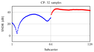
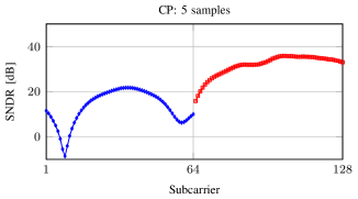
Figure 12: Theoretic (line) and empirical (markers) SNDR for a CP-OFDMA channel with two users. The SNR for both users is set to 40 dB. The channel impulse responses are 14-tap long and correspond to the realizations of Fig. 7. The length of the cyclic prefix is either 32 samples (top) or 5 samples (bottom).

As a final remark, it is interesting to see that (23) takes the form

$$P_{e,k}^{\text{(CP)}}(m)=P_{s}\frac{|W_{m}|^{2}}{2M^{2}}\sum_{\ell=m_{\min}}^{m_{\max}}\frac{\sin^{2}\bigl{[}\frac{\pi}{2M}(m-\ell)(L_{T}-1)\bigr{]}}{\sin^{2}\bigl{[}\frac{\pi}{2M}(m-\ell)\bigr{]}}$$

when User $k$ transmits over subcarriers $\{m_{\min},\dots,m_{\max}\}$ at power $P_{s}$ and when its channel is a delay of $L_{T}-1$ samples (i.e., the channel impulse response is $\delta[n-L_{T}]$). Note that this is the case considered in Section IV-B.

References

- [1] A. Goldsmith, Wireless Communications. New York, NY, USA: Cambridge University Press, 2005.
- [2] 3rd Generation Partnership Project, “LTE; Evolved Universal Terrestrial Radio Access (E-UTRA); Physical Channels and Modulation,” ETSI, Tech. Spec. TS36.211 v12.5.0 release 12, 2015.
- [3] M. Morelli, C.-C. J. Kuo, and M.-O. Pun, “Synchronization techniques for orthogonal frequency division multiple access (OFDMA): A tutorial review,” Proc. IEEE, vol. 95, no. 7, pp. 1394–1427, Jul. 2007.
- [4] S. B. Weinstein and P. M. Ebert, “Data transmission by frequency-division multiplexing using the discrete Fourier transform,” IEEE Trans. Commun. Technol., vol. COM-19, no. 5, pp. 628–634, Oct. 1971.
- [5] P. P. Vaidyanathan, “Filter banks in digital communications,” IEEE Circuits Syst. Mag., vol. 1, no. 2, pp. 4–25, Second Quarter 2001.
- [6] B. Farhang-Boroujeny, “OFDM versus filter bank multicarrier,” IEEE Signal Process. Mag., vol. 28, no. 3, pp. 92–112, May 2011.
- [7] D. Roque, C. Siclet, and P. Siohan, “A performance comparison of FBMC modulation schemes with short perfect reconstruction filters,” in Proc. IEEE ICT 2012, Jounieh, Lebanon, Apr. 23–25 2012.
- [8] T. Ihalainen, T. H. Stitz, M. Rinne, and M. Renfors, “Channel equalization in filter bank based multicarrier modulation for wireless communications,” EURASIP J. Adv. Signal Process., vol. 2007, 2007.
- [9] D. S. Waldhauser, L. G. Baltar, and J. A. Nossek, “MMSE subcarrier equalization for filter bank based multicarrier systems,” in Proc. IEEE SPAWC 2008, Recife, Brazil, Jul. 6–9 2008.
- [10] G. Ndo, H. Lin, and P. Siohan, “FBMC/OQAM equalization: Exploiting the imaginary interference,” in Proc. IEEE PIMRC 2012, Sydney, Australia, Sep. 9–12 2012.
- [11] X. Mestre, M. Majoral, and S. Pfletschinger, “An asymptotic approach to parallel equalization of filter bank based multicarrier signals,” IEEE Trans. Signal Process., vol. 61, no. 14, pp. 3592–3606, Jul. 2013.
- [12] H. Saeedi-Sourck, Y. Wu, J. W. M. Bergmans, S. Sadri, and B. Farhang-Boroujeny, “Complexity and performance comparison of filter bank multicarrier and OFDM in uplink of multicarrier multiple access networks,” IEEE Trans. Signal Process., vol. 59, no. 4, pp. 1907–1912, Apr. 2011.
- [13] D. Mattera, M. Tanda, and M. Bellanger, “Performance analysis of some timing offset equalizers for FBMC/OQAM systems,” Signal Processing, vol. 108, pp. 167–182, 2015.
- [14] T. Ihalainen, A. Viholainen, T. H. Stitz, M. Renfors, and M. Bellanger, “Filter bank based multi-mode multiple access scheme for wireless uplink,” in Proc. EUSIPCO 2009, Glasgow, Scotland, Aug. 24–28 2009.
- [15] D. Mattera, M. Tanda, and M. Bellanger, “Analysis of an FBMC/OQAM scheme for asynchronous access in wireless communications,” EURASIP J. Adv. Signal Process., vol. 2015, no. 23, 2015.
- [16] P. Siohan, C. Siclet, and N. Lacaille, “Analysis design of OFDMA/OQAM systems based on filterbank theory,” IEEE Trans. Signal Process., vol. 50, no. 5, pp. 1170–1183, May 2002.
- [17] C. Siclet, P. Siohan, and D. Pinchon, “Perfect reconstruction conditions and design of oversampled DFT-modulated transmultiplexers,” EURASIP Journal on Advances in Signal Processing, vol. 2006, no. 1, pp. 1–15, 2006.
- [18] P. Amini, R.-R. Chen, and B. Farhang-Boroujeny, “Filterbank multicarrier communications for underwater acoustic channels,” IEEE J. Ocean. Eng., vol. 40, no. 1, pp. 115–130, Jan. 2015.
- [19] M. Bellanger, “FS-FBMC: An alternative scheme for filter bank based multicarrier transmission,” in Proc. IEEE ISCCSP 2012, Rome, Italy, May 2–4 2012.
- [20] D. Mattera, M. Tanda, and M. Bellanger, “Frequency-spreading implementation of OFDM/OQAM systems,” in Proc. IEEE ISWCS 2012, Paris, France, Aug. 28–31 2012.
- [21] M. Renfors, J. Yli-Kaakinen, and fredric j. harris, “Analysis and design of efficient and flexible fast-convolution based multirate filter banks,” IEEE Trans. Signal Process., vol. 62, no. 15, pp. 3768–3783, Aug. 2014.
- [22] B. Farhang-Boroujeny, “Filter bank spectrum sensing for cognitive radios,” IEEE Trans. Signal Process., vol. 56, no. 5, pp. 1801–1811, May 2008.
- [23] A. Viholainen et al., “Prototype filter and structure optimization,” Project PHYDYAS ICT-211887, Deliverable D5.1, Jan. 2009.
- [24] S. Mirabbasi and K. Martin, “Overlapped complex-modulated transmultiplexer filters with simplified design and superior stopbands,” IEEE Trans. Circuits Syst. II, vol. 50, no. 8, pp. 456–469, Aug. 2003.
- [25] R. Li and G. Stette, “Time-limited orthogonal multicarrier modulation schemes,” IEEE Trans. Commun., vol. 43, no. 2/3/4, pp. 1269–1272, Feb. 1995.
- [26] 3rd Generation Partnership Project, “Evolved Universal Terrestrial Radio Access (E-UTRA); User Equipment (UE) Radio Transmission and Reception,” ETSI, Tech. Rep. TR36.803 v1.1.0 release 8, 2008.
- [27] S. Benedetto and E. Biglieri, Principles of Digital Transmission: With Wireless Applications. New York, NY, USA: Kluwer Academic / Plenum Publishers, 1999.