Distributed Randomized Control
for Demand Dispatch

Abstract

The paper concerns design of control systems for Demand Dispatch to obtain ancillary services to the power grid by harnessing inherent flexibility in many loads. The role of “local intelligence” at the load has been advocated in prior work; randomized local controllers that manifest this intelligence are convenient for loads with a finite number of states. The present work introduces two new design techniques for these randomized controllers:

• The Individual Perspective Design (IPD) is based on the solution to a one-dimensional family of Markov Decision Processes, whose objective function is formulated from the point of view of a single load. The family of dynamic programming equation appears complex, but it is shown that it is obtained through the solution of a single ordinary differential equation.

• The System Perspective Design (SPD) is motivated by a single objective of the grid operator: Passivity of any linearization of the aggregate input-output model. A solution is obtained that can again be computed through the solution of a single ordinary differential equation.

Numerical results complement these theoretical results.

1 Introduction

Renewable energy sources such as wind and solar power have a high degree of unpredictability and time variation, which makes balancing demand and supply increasingly challenging. One way to address this challenge is to harness the inherent flexibility in demand of many types of loads. Loads can supply a range of ancillary services to the grid, such as the balancing reserves required at Bonneville Power Authority (BPA), or the Reg-D/A regulation reserves used at PJM [1]. Today these services are secured by a balancing authority (BA) in each region.

1.1 Demand dispatch

These grid services can be obtained without impacting quality of service (QoS) for consumers [2, 1], but this is only possible through design. The term Demand Dispatch is used in this paper to emphasize the difference between the goals of our own work and traditional demand response.

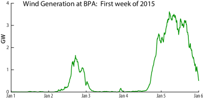
Figure 1: Wind generation at BPA.

Consumers use power for a reason, and expect some guarantees on the QoS they receive. The grid operator desires reliable ancillary service, obtained from the inherent flexibility in the consumer’s power consumption. These seemingly conflicting goals can be achieved simultaneously, but the solution requires local control: an appliance must monitor its QoS and other state variables, it must receive grid-level information (e.g., from the BA), and based on this information it must adjust its power consumption. With proper design, an aggregate of loads can be viewed at the grid-level as virtual energy storage (VES). Just like a battery, the aggregate provides ancillary service, even though it cannot produce energy.

Fig. 1 shows the wind generation in the BPA region during the first week of 2015. There is virtually no power generated on New Year’s Day, and generation ramps up to nearly 4GW on the morning of January 5. In this example we show how to supply a demand of exactly 4GW during this time period, using generation from wind and other resources.

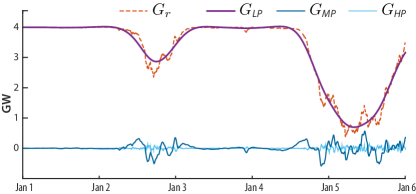
Figure 2: One power signal representing significant energy delivery, and two zero-energy power signals combine with wind generation to match a 4GW load.

Let $G_{r}(t)$ denote the additional power required at time $t$, in units of GWs. For example, on the first day of this week we have $G_{r}(t)\approx 4$. Day-ahead forecast of the low frequency component of generation from wind is highly predictable. We let $G_{\text{\it LP}}$ denote the signal obtained by passing the forecast of $G_{r}$ through a low pass filter. The signal $G_{\text{\it HP}}$ is obtained by filtering $G_{r}-G_{\text{\it LP}}$ using a high pass filter, and $G_{\text{\it MP}}=G_{r}-G_{\text{\it LP}}-G_{\text{\it HP}}$. Each of these filters is causal, and their parameters are a design choice. Examples are shown in Fig. 2.

It is not difficult to ramp hydro-generation up and down to accurately track the power signal $G_{\text{\it LP}}$. This is an energy product that might be secured in today’s day-ahead markets.

The other two signals shown in Fig. 2 take on positive and negative values. Each represents a total energy of approximately zero, hence it would be a mistake to attempt to obtain these services in an energy market. Either could be obtained from a large fleet of batteries or flywheels. However, it may be much cheaper to employ flexible loads via demand dispatch. The signal $G_{\text{\it HP}}$ can be obtained by modulating the fans in commercial buildings (perhaps by less than 10%) [3]. The signal $G_{\text{\it MP}}$ can be supplied in whole or in part by loads such as water heaters, commercial refrigeration, and water chillers.

Low frequency variability from solar gives rise to the famous “duck curve” anticipated at CAISO, which is represented as the hypothetical “net-load curve” in Fig. 3(a). The actual net-load curve is the difference between load and generation from renewables; the drop from 20 to 10 GW is expected with the introduction of 10 GW of solar in the state of California. This curve highlights the ramping pressure placed on conventional generation resources.

As shown in this figure, the volatility and steep ramps associated with California’s duck curve can be addressed using a frequency decomposition: The plot shows how the net-load can be expressed as the sum of four signals distinguished by frequency. Variability introduced by the low frequency component can be rejected using traditional resources such as thermal generators, along with some flexible loads (e.g., from flexible industrial manufacturing). The mid-pass signal shown in the figure would be a challenge to generators for various reasons, but this zero-mean signal, as well as the higher frequency components, can be tracked using a variety of flexible loads.

The control architecture described in this paper is not limited to handling disturbances from wind and solar energy. Fig. 3(b) illustrates how the same frequency decomposition can be used to allocate resources following an unexpected contingency, such as a generator outage.

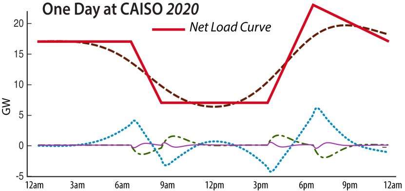
(a) The “duck curve” is decomposed as the sum of four signals: The three high-frequency components can be obtained using VES.

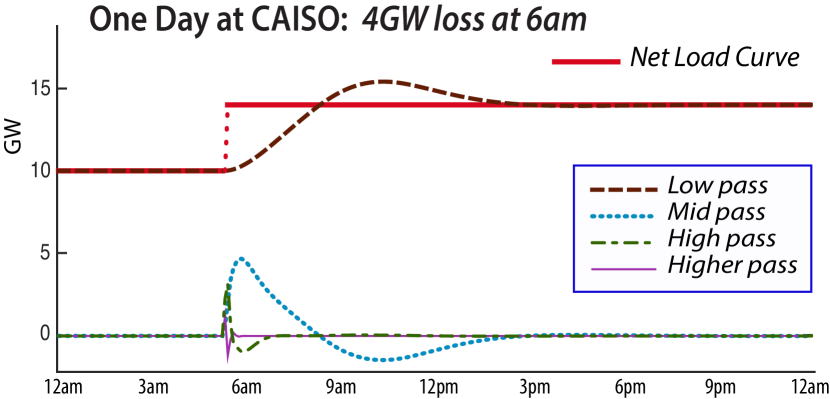
(b) An unexpected power outage requires quick ramping of power generation. The zero-energy components are obtained using VES.

Figure 3: Frequency decomposition in two examples in which large ramps in generation are required. In each case, the low-pass energy component can be obtained through conventional generation, or load-shedding. The remaining components of net-load are obtained using VES.

For loads whose power consumption cannot be varied continuously, we have argued in prior work that a distributed randomized control architecture is convenient for design [4, 2, 5]. This architecture includes local control to maintain bounds on the quality of service delivered by the loads, and also to ensure high quality ancillary service to the grid.

Analysis of the aggregate is based on a mean-field model.

1.2 Mean-field model

We restrict to the setting of the prior work [4, 2], based on the following distributed control architecture. A family of transition matrices $\{P_{\zeta}:\zeta\in\mathbb{R}\}$ is constructed to define local decision making. Each load evolves as a controlled Markov chain on a finite state space, with common input ${\mathchoice{\mbox{\boldmath$\zeta$}}{\mbox{\boldmath$\zeta$}}{\mbox{\boldmath$\scriptstyle\zeta$}}{\mbox{\boldmath$\scriptscriptstyle\zeta$}}}=(\zeta_{0},\zeta_{1},\dots)$. it is assumed that the scalar signal $\zeta$ is broadcast to each load. If a load is in state $x$ at time $t$, and the value $\zeta_{t}$ is broadcast, then the load transitions to the state $x^{\prime}$ with probability $P_{\zeta_{t}}(x,x^{\prime})$. Letting $X^{i}_{t}$ denote the state of the $i$th load at time $t$, and assuming $N$ loads, the empirical pdf (probability mass function) is defined as the average,

$$\mu^{N}_{t}(x)=\frac{1}{N}\sum_{i=1}^{N}\mathbb{I}\{X^{i}_{t}=x\},\qquad x\in{\sf X}.$$

The mean-field model is the deterministic system defined by the evolution equations,

$$\mu_{t+1}=\mu_{t}P_{\zeta_{t}},\quad t\geq 0,$$ (1)

in which $\mu_{t}$ is a row vector. Under general conditions on the model and on $\mu_{0}$ it can be shown that $\mu^{N}_{t}$ is approximated by $\mu_{t}$.

In this prior work it is assumed that average power consumption is obtained through measurements or state estimation: Assume that $\mathchoice{\mbox{\small$\cal U$}}{\mbox{\small$\cal U$}}{\mbox{$\scriptstyle\cal U$}}{\mbox{$\scriptscriptstyle\cal U$}}(x)$ is the power consumption when the load is in state $x$, for some function $\mathchoice{\mbox{\small$\cal U$}}{\mbox{\small$\cal U$}}{\mbox{$\scriptstyle\cal U$}}{\mbox{$\scriptscriptstyle\cal U$}}\colon{\sf X}\to\mathbb{R}_{+}$. The average power consumption is defined by,

$$y^{N}_{t}=\frac{1}{N}\sum_{i=1}^{N}\mathchoice{\mbox{\small$\cal U$}}{\mbox{\small$\cal U$}}{\mbox{$\scriptstyle\cal U$}}{\mbox{$\scriptscriptstyle\cal U$}}(X^{i}_{t}),\qquad x\in{\sf X}.$$

which is approximated using the mean-field model:

$$y_{t}=\sum_{x}\mu_{t}(x)\mathchoice{\mbox{\small$\cal U$}}{\mbox{\small$\cal U$}}{\mbox{$\scriptstyle\cal U$}}{\mbox{$\scriptscriptstyle\cal U$}}(x),\quad t\geq 0.$$ (2)

The mean-field model is a state space model that is linear in the state $\mu_{t}$, and nonlinear in the input $\zeta_{t}$. The observation process (2) is also linear as a function of the state. Assumptions imposed in the prior work [2, 5, 4] imply that the input is a continuous function of these values.

In [4], the design of the feedback law $\zeta_{t}=\phi_{t}(y_{0},\dots,y_{t})$ is based on a linearization of this state space model. One goal of the present paper is to develop design techniques to ensure that the linearized input-output model has desirable properties for control design at the grid level.

1.3 Contributions

Several new design techniques are introduced in this paper, and the applications go far beyond prior work:

• Optimal design. In the prior work [4], the family of transition matrices $\{P_{\zeta}\}$ was constructed based on an average-cost optimal control problem (MDP). The cost function in this MDP was parameterized by the scalar $\zeta$. In this prior work, the optimal control problem was completely unconstrained, in the sense that any choice of $P$ was permissible in the optimal control formulation. The optimal control formulation proposed here is far more general: We allow some randomness by design, and some exogenous randomness that is beyond our control. These contributions are summarized in Theorem 2.2.

• Passivity by design. A discrete-time transfer function $F$ is positive-real if it is stable (all poles are strictly within the unit disk), and the following bound holds:

  $$F(e^{j\theta})+F(e^{-j\theta})\geq 0,\quad\theta\in\mathbb{R}$$

  It is strictly positive-real if the inequality is strict for all $\theta$. A linear system is passive if it is positive real.

  Let $(A,B,C)$ describe a state-space representative of the linearization, with transfer function $G(z)=C(Iz-A]^{-1}B$. Consider the delay-free model with transfer function $G^{+}(z)\mathbin{:=}zG(z)$. That is,

  $$G^{+}(z)=zC[Iz-A]^{-1}B=\sum_{k=0}^{\infty}CA^{k}Bz^{-k}$$ (3)

  A new approach to design of the transition matrices is introduced in this paper to ensure that the linearization is strictly positive real. The main conclusions are summarized in Theorem 2.3.

• ODE methods for design. A unified computational framework is introduced. The construction of the transition matrices $\{P_{\zeta}:\zeta\in\mathbb{R}\}$ is obtained as the solution to a single ODE for each of the design techniques (i) and (ii).

• Applications. Prior work on distributed control for demand dispatch focused on a single collection of loads: residential pool pumps [6, 4, 5]. The motivation was ease of exposition, and also the fact that the design methodology required special assumptions on nominal behavior. The new methodology developed in this paper relaxes these assumptions, and allows application to any load with discrete power states, such as a refrigerator, or other thermostatically controlled loads (TCLs).

1.4 Prior work

There are many recent papers with similar goals – to create a science to support demand dispatch. In [7] and its sequels, all control decisions are at the balancing authority, and this architecture then requires state estimation to obtain the grid-level control law. A centralized deterministic approach is developed in [8, 9]. None of this prior work considers design of local control algorithms, which is the focus of this paper.

Passivity was established in the prior work [10], but only for continuous time models for which the nominal model (with $\zeta=0$) is a reversible Markov process. It follows that $G^{+}$ is minimum phase, and hence the original transfer function $G(z)=z^{-1}G^{+}(z)$ is also minimum phase.

The remainder of the paper is organized into four sections. Several design techniques are introduced in Section 2, and Section 3 presents general methodology for constructing and analyzing the linearized mean-field dynamics. Examples are contained in Section 4, and conclusions in Section 5.

2 Design

We first summarize the assumptions and notation.

2.1 Assumptions and Notation

A Markovian model for an individual load is created based on its typical operating behavior. This is modeled by a Markov chain with transition matrix denoted $P_{0}$, with state space ${\sf X}=\{x^{1},\dots,x^{d}\}$; it is assumed to be irreducible and aperiodic. It follows that $P_{0}$ admits a unique invariant pmf (probability mass function), denoted $\pi_{0}$, and satisfying $\pi_{0}(x)>0$ for each $x$.

It is assumed throughout this paper that the family of transition matrices used for distributed control is of the form,

$$P_{\zeta}(x,x^{\prime})\mathbin{:=}P_{0}(x,x^{\prime})\exp\bigl{(}h_{\zeta}(x,x^{\prime})-\Lambda_{h_{\zeta}}(x)\bigr{)}$$ (4)

in which $h_{\zeta}$ is continuously differentiable in $\zeta$, and $\Lambda_{h_{\zeta}}$ is the normalizing constant

$$\Lambda_{h_{\zeta}}(x)\mathbin{:=}\log\Bigl{(}\sum_{x^{\prime}}P_{0}(x,x^{\prime})\exp\bigl{(}h_{\zeta}(x,x^{\prime})\bigr{)}\Bigr{)}$$ (5)

Each $P_{\zeta}$ must also be irreducible and aperiodic.

For any transition matrix $P$, an invariant pmf is interpreted as a row vector, so that invariance can be expressed $\pi P=\pi$. Any function $f\colon{\sf X}\to\mathbb{R}$ is interpreted as a $d$-dimensional column vector, and we use the standard notation $Pf\,(x)=\sum_{x^{\prime}}P(x,x^{\prime})f(x^{\prime})$, $x\in{\sf X}$.

Several other matrices are defined based on $P$ and $\pi$: The adjoint of $P$ (in $L_{2}(\pi)$) is the transition matrix defined by

$$P^{\Lsh}(x,x^{\prime})=\frac{\pi(x^{\prime})}{\pi(x)}P(x^{\prime},x),\quad x,x^{\prime}\in{\sf X}.$$ (6)

The fundamental matrix is the inverse

$$Z=[I-P+1\otimes\pi]^{-1}=\sum_{n=0}^{\infty}[P-1\otimes\pi]^{n}$$ (7)

with $[P-1\otimes\pi]^{0}\mathbin{:=}I$ (the $d\times d$ identity matrix), $1\otimes\pi$ is a matrix in which each row is identical, and equal to $\pi$, and $[P-1\otimes\pi]^{n}=P^{n}-1\otimes\pi$ for $n\geq 1$.

The Donsker-Varadhan rate function is denoted,

$$K(P\|P_{0})=\sum_{x,x^{\prime}}\pi(x)P(x,x^{\prime})\log\Bigl{(}\frac{P(x,x^{\prime})}{P_{0}(x,x^{\prime})}\Bigr{)}$$ (8)

It is used here to model the cost of deviation from the nominal transition matrix $P_{0}$, as in [11, 12, 4, 10].

Nature & nurture

In many applications it is necessary to include a model of randomness from nature along with the randomness introduced by the local control algorithm (nurture).

Consider a load model in which the full state space is the cartesian product of two finite state spaces: ${\sf X}={\sf X}_{\sf u}\times{\sf X}_{\sf n}$, where ${\sf X}_{\sf u}$ are components of the state that can be directly manipulated through control. The “nature” components ${\sf X}_{\sf n}$ are not subject to direct control. For example, these components may be used to model the impact of the weather on the climate of a building.

Elements of ${\sf X}$ are denoted $x=(x_{u},x_{n})$. Any state transition matrix under consideration is assumed to have the following conditional-independence structure,

$$P(x,x^{\prime})=R(x,x_{u}^{\prime})Q_{0}(x,x_{n}^{\prime}),$$ (9)

for $x\in{\sf X},x_{u}^{\prime}\in{\sf X}_{\sf u},\ x_{n}^{\prime}\in{\sf X}_{\sf n}$, where $\sum_{x_{u}^{\prime}}R(x,x_{u}^{\prime})=\sum_{x_{n}^{\prime}}Q_{0}(x,x_{n}^{\prime})=1$ for each $x$. The matrix $Q_{0}$ is out of our control – this models load dynamics and exogenous disturbances.

2.2 Common structure for design

The construction of the family of functions $\{h_{\zeta}:\zeta\in\mathbb{R}\}$ in (4) is achieved using the following steps.

Step 1: The specification of a function ${\cal H}$ that takes as input a transition matrix $P$ that is irreducible. The output $H={\cal H}(P)$ is a real-valued function on the product space ${\sf X}\times{\sf X}$. That is, $H(x,x^{\prime})\in\mathbb{R}$ for each pair $(x,x^{\prime})\in{\sf X}\times{\sf X}$.

Step 2: The family of transition matrices $\{P_{\zeta}\}$ and functions $\{h_{\zeta}\}$ are defined by the solution to the $d$-dimensional ODE:

$${\mathchoice{\genfrac{}{}{}{1}{d}{d\zeta}}{\genfrac{}{}{}{1}{d}{d\zeta}}{\genfrac{}{}{}{3}{d}{d\zeta}}{\genfrac{}{}{}{3}{d}{d\zeta}}}h_{\zeta}={\cal H}(P_{\zeta}),\qquad\zeta\in\mathbb{R},$$ (10)

in which $P_{\zeta}$ is determined by $h_{\zeta}$ through (4). The boundary condition for this ODE is $h_{0}\equiv 0$.

In the special case in which randomness from nature is not considered, we can apply the methods described here using ${\sf X}_{\sf n}=\{x_{n}^{1}\}$ (a singleton).

The conditional independence constraint (9) imposes constraints on the functions $\{h_{\zeta}\}$ and the transformation ${\cal H}$. To ensure that $P_{\zeta}$ is of the form (9), it is sufficient to restrict to functions $h_{\zeta}$ of $(x,x^{\prime})$ that do not depend on $x_{n}^{\prime}$, where $x^{\prime}=(x_{u}^{\prime},x_{n}^{\prime})\in{\sf X}$. For this reason we make the notational convention,

$$h_{\zeta}(x,x^{\prime})=h_{\zeta}(x,x_{u}^{\prime}),\qquad x\in{\sf X},\ x^{\prime}=(x_{u}^{\prime},x_{n}^{\prime})\in{\sf X}.$$

Since $h_{\zeta}$ is constructed through the ODE (10), we impose the same constraints on $H={\cal H}(P)$:

$$H(x,x^{\prime})=H(x,x_{u}^{\prime}),\qquad x\in{\sf X},\ x^{\prime}=(x_{u}^{\prime},x_{n}^{\prime})\in{\sf X}.$$

Given any function $H^{\circ}\colon{\sf X}\to\mathbb{R}$, the function defined below satisfies this constraint:

$$H(x,x^{\prime}_{u})=\sum_{x_{n}^{\prime}}Q_{0}(x,x_{n}^{\prime})H^{\circ}(x_{u}^{\prime},x_{n}^{\prime})$$ (11)

Each of the methods that follow construct $H={\cal H}(P)$ of this form. Hence the design problem reduces to choosing a mapping $H^{\circ}={\cal H}^{\circ}(P)$.

The following normalization is imposed throughout: The transition matrix $P_{\zeta}$ defined in (4) does not change if we add a constant to the function $h_{\zeta}$. We are thus free to normalize $H^{\circ}={\cal H}^{\circ}(P)$ by a constant. Throughout the paper we fix a state $x^{\circ}\in{\sf X}$, and design ${\cal H}^{\circ}$ so that $H^{\circ}(x^{\circ})=0$ for any $P$.

The ODE method can be simplified based on these observations. The proof of Prop. 2.1 is straightforward.

Proposition 2.1.

Consider a solution to the ODE (10) in which $H={\cal H}(P)$ is of the form (11) for any matrix $P$. It then follows that each of the functions $\{h_{\zeta}\}$ are of this form:

$$h_{\zeta}(x,x^{\prime}_{u})=\sum_{x_{n}^{\prime}}Q_{0}(x,x_{n}^{\prime})h_{\zeta}^{\circ}(x_{u}^{\prime},x_{n}^{\prime}),$$

$x\in{\sf X},\ x^{\prime}=(x_{u}^{\prime},x_{n}^{\prime})\in{\sf X}$, for some $h_{\zeta}^{\circ}\colon{\sf X}\to\mathbb{R}$. Moreover, these functions solve the $d$-dimensional ODE,

$${\mathchoice{\genfrac{}{}{}{1}{d}{d\zeta}}{\genfrac{}{}{}{1}{d}{d\zeta}}{\genfrac{}{}{}{3}{d}{d\zeta}}{\genfrac{}{}{}{3}{d}{d\zeta}}}h_{\zeta}^{\circ}={\cal H}^{\circ}(P_{\zeta}),\qquad\zeta\in\mathbb{R},$$

in which $P_{\zeta}$ is determined by $h_{\zeta}$ through (4), and with boundary condition $h_{0}^{\circ}\equiv 0$.      

2.3 Individual Perspective

In this design, the mapping $H^{\circ}={\cal H}^{\circ}(P)$ is defined in terms of the fundamental matrix:

IPD solution:   Given $P$, the fundamental matrix $Z$ is obtained from (7), and then for each $x\in{\sf X}$,

$$H^{\circ}(x)=\sum_{x^{\prime}}[Z(x,x^{\prime})-Z(x^{\circ},x^{\prime})]\mathchoice{\mbox{\small$\cal U$}}{\mbox{\small$\cal U$}}{\mbox{$\scriptstyle\cal U$}}{\mbox{$\scriptscriptstyle\cal U$}}(x^{\prime}).$$ (12)

The function $H^{\circ}$ specified in (12) is a solution to Poisson’s equation,

$$PH^{\circ}=H^{\circ}-\mathchoice{\mbox{\small$\cal U$}}{\mbox{\small$\cal U$}}{\mbox{$\scriptstyle\cal U$}}{\mbox{$\scriptscriptstyle\cal U$}}+\mbox{\scriptsize$\bar{\cal U}$}$$ (13)

where $\bar{\cal U}$ (also written $\pi(\mathchoice{\mbox{\small$\cal U$}}{\mbox{\small$\cal U$}}{\mbox{$\scriptstyle\cal U$}}{\mbox{$\scriptscriptstyle\cal U$}})$) is the steady-state mean:

$$\mbox{\scriptsize$\bar{\cal U}$}\mathbin{:=}\sum_{x}\pi(x)\mathchoice{\mbox{\small$\cal U$}}{\mbox{\small$\cal U$}}{\mbox{$\scriptstyle\cal U$}}{\mbox{$\scriptscriptstyle\cal U$}}(x)$$ (14)

The function (12) is the unique solution satisfying $H^{\circ}(x^{\circ})=0$ [13, Thm. 17.7.2].

This choice for $H^{\circ}$ is called the Individual Perspective Design (IPD) since $h_{\zeta}$ solves an optimization problem formulated from the point of view of a single load. Given $\zeta\in\mathbb{R}$, the “optimal reward” is defined by the maximum,

$$\eta^{*}_{\zeta}=\max_{\pi,P}\bigl{\{}\zeta\pi(\mathchoice{\mbox{\small$\cal U$}}{\mbox{\small$\cal U$}}{\mbox{$\scriptstyle\cal U$}}{\mbox{$\scriptscriptstyle\cal U$}})-K(P\|P_{0}):\pi P=\pi\bigr{\}}$$ (15)

and $P$ is also subject to the structural constraint (9). The maximizer defines a transition matrix that is denoted,

$${\check{P}}_{\zeta}=\mathop{\rm arg\,max}_{P}\bigl{\{}\zeta\pi(\mathchoice{\mbox{\small$\cal U$}}{\mbox{\small$\cal U$}}{\mbox{$\scriptstyle\cal U$}}{\mbox{$\scriptscriptstyle\cal U$}})-K(P\|P_{0}):\pi P=\pi\bigr{\}}$$ (16)

It is shown in Theorem 2.2 that the optimal value $\eta^{*}_{\zeta}$ together with a relative value function $h^{*}_{\zeta}$ solve the average reward optimization equation (AROE):

$$\max_{P}\Bigl{\{}{\cal W}_{\zeta}(x,P)+\sum_{x^{\prime}}P(x,x^{\prime})h^{*}_{\zeta}(x^{\prime})\Bigr{\}}=h^{*}_{\zeta}(x)+\eta^{*}_{\zeta}$$ (17)

where ${\cal W}_{\zeta}(x,P)=\zeta\mathchoice{\mbox{\small$\cal U$}}{\mbox{\small$\cal U$}}{\mbox{$\scriptstyle\cal U$}}{\mbox{$\scriptscriptstyle\cal U$}}(x)-\sum_{x^{\prime}}P(x,x^{\prime})\log\bigl{(}\frac{P(x,x^{\prime})}{P_{0}(x,x^{\prime})}\bigr{)}$.

The relative value function is not unique, since we can add a constant to obtain a new solution. We normalize this function so that $h^{*}_{\zeta}(x^{\circ})=0$. The proof of the following can be found in the working paper [14].

Theorem 2.2.

The IPD solution results in a collection of transition matrices $\{P_{\zeta}:\zeta\in\mathbb{R}\}$ with the following properties. For each $\zeta$,

• The transition matrix is optimal, $P_{\zeta}={\check{P}}_{\zeta}$.

• For each $x$ and $x_{u}^{\prime}$, the function $h_{\zeta}$ that defines $P_{\zeta}$ is given by,

  $$h_{\zeta}(x,x^{\prime}_{u})=\sum_{x_{n}^{\prime}}Q_{0}(x,x_{n}^{\prime})h^{*}_{\zeta}(x_{u}^{\prime},x_{n}^{\prime})$$ (18)

  where $(h^{*}_{\zeta},\eta^{*}_{\zeta})$ solves the AROE (17).

• The steady-state mean power consumption satisfies,

  $${\mathchoice{\genfrac{}{}{}{1}{d}{d\zeta}}{\genfrac{}{}{}{1}{d}{d\zeta}}{\genfrac{}{}{}{3}{d}{d\zeta}}{\genfrac{}{}{}{3}{d}{d\zeta}}}\mbox{\scriptsize$\bar{\cal U}$}_{\zeta}=\genfrac{}{}{}{1}{d^{2}}{d\zeta^{2}}\eta^{*}_{\zeta}\geq 0$$ (19)

  and hence $\mbox{\scriptsize$\bar{\cal U}$}_{\zeta}$ is monotone in $\zeta$.      

2.4 System Perspective

The motivation for the following System Perspective Design (SPD) is from the point of view of the BA. Under general conditions, the linearized aggregate model is passive, which is a desirable property from the grid-level perspective.

The construction of $H^{\circ}={\cal H}^{\circ}(P)$ is similar to IPD. For any matrix $P$ with invariant pmf $\pi$, recall the definition of the adjoint $P^{\Lsh}$ in (6). The matrix product is denoted

$$P^{\triangledown}(x,x^{\prime})=\sum_{z\in{\sf X}}P^{\Lsh}(x,z)P(z,x^{\prime}),\qquad x,x^{\prime}\in{\sf X}.$$

The fundamental matrix defined in terms of this transition matrix is denoted $Z^{\triangledown}=[I-P^{\triangledown}+1\otimes\pi]^{-1}$.

SPD solution:   Given $P$, the matrix $Z^{\triangledown}$ is obtained, and

$$\!\!H^{\circ}(x)=\sum_{x^{\prime}}[Z^{\triangledown}(x,x^{\prime})-Z^{\triangledown}(x^{\circ},x^{\prime})]\mathchoice{\mbox{\small$\cal U$}}{\mbox{\small$\cal U$}}{\mbox{$\scriptstyle\cal U$}}{\mbox{$\scriptscriptstyle\cal U$}}(x^{\prime})\,,\ \ x\in{\sf X}.$$ (20)

Under additional assumptions, the algorithm obtained from SPD results in a positive real linearization. The proof of the bound (21) is contained in Section 3.2.

Theorem 2.3.

Suppose that the Markov chain with transition matrix $P^{\triangledown}_{0}=P_{0}^{\Lsh}P_{0}$ is irreducible, and that $P_{0}=R_{0}$ (a model without probabilistic constraints).

Then, the solution to the SPD satisfies the following strict positive-real condition: the linearized model at any constant value $\zeta$ obeys the bound,

$$G^{+}_{\zeta}(e^{j\theta})+G^{+}_{\zeta}(e^{-j\theta})\geq\sigma^{2}_{\zeta},\qquad\theta\in\mathbb{R}$$ (21)

where $\sigma^{2}_{\zeta}$ is the variance of $\cal U$ under $\pi_{\zeta}$.      

The irreducibility assumption on $P^{\triangledown}_{0}$ does not come for free. Consider for example the Markov chain on $d\geq 3$ states defined by $P_{0}(x^{i},x^{i+1})=1$ for $1\leq i\leq d-1$, and $P_{0}(x^{d},x^{d})=P_{0}(x^{d},x^{1})=1/2$. This chain is irreducible and aperiodic. The behavior of the adjoint is similar; in particular, $P_{0}^{\Lsh}(x^{i+1},x^{i})=1$ for each $1\leq i\leq d-1$. It follows that $P^{\triangledown}_{0}(x^{k},x^{k})=1$ for $2\leq k\leq d$, so the irreducibility assumption fails.

2.5 Exponential family

Rather than solve an ODE, it is natural to fix a function $H_{\text{\rm\scriptsize e}}^{\circ}\colon{\sf X}\to\mathbb{R}$, and define for each $x,x^{\prime}_{u}$ and $\zeta$,

$$h_{\zeta}(x,x^{\prime}_{u}) =\zeta H_{\text{\rm\scriptsize e}}(x_{u}^{\prime}\mid x)$$

$$\text{with}\quad H_{\text{\rm\scriptsize e}}(x_{u}^{\prime}\mid x) \mathbin{:=}\sum_{x_{n}^{\prime}}Q_{0}(x,x_{n}^{\prime})H_{\text{\rm\scriptsize e}}^{\circ}(x_{u}^{\prime},x_{n}^{\prime})$$

This is a special case of the two-step design described in Section 2.2 in which ${\cal H}^{\circ}(P)=H_{\text{\rm\scriptsize e}}^{\circ}$, independent of $P$, and the function $H={\cal H}(P)$ is then obtained from (11).

In this case, the transition matrices defined in (4) can be regarded as an exponential family. The exponential family using $H_{\text{\rm\scriptsize e}}^{\circ}=\mathchoice{\mbox{\small$\cal U$}}{\mbox{\small$\cal U$}}{\mbox{$\scriptstyle\cal U$}}{\mbox{$\scriptscriptstyle\cal U$}}$ will be called the myopic design.

Other designs can be obtained as linear approximations to the IPD or SPD solutions, with $H_{\text{\rm\scriptsize e}}^{\circ}={\cal H}^{\circ}(P_{0})$. In the linear approximation of the IPD solution, this is a solution Poisson’s equation for the nominal model:

$$P_{0}H_{\text{\rm\scriptsize e}}^{\circ}=H_{\text{\rm\scriptsize e}}^{\circ}-\mathchoice{\mbox{\small$\cal\widetilde{U}$}}{\mbox{\small$\cal\widetilde{U}$}}{\mbox{$\scriptstyle\cal\widetilde{U}$}}{\mbox{$\scriptscriptstyle\cal\tilde{U}$}}_{0}$$ (22)

where $\mathchoice{\mbox{\small$\cal\widetilde{U}$}}{\mbox{\small$\cal\widetilde{U}$}}{\mbox{$\scriptstyle\cal\widetilde{U}$}}{\mbox{$\scriptscriptstyle\cal\tilde{U}$}}_{0}(x)=\mathchoice{\mbox{\small$\cal U$}}{\mbox{\small$\cal U$}}{\mbox{$\scriptstyle\cal U$}}{\mbox{$\scriptscriptstyle\cal U$}}(x)-\mbox{\scriptsize$\bar{\cal U}$}_{0}$. The resulting exponential family is called the IPD₀ design. It is approximately optimal for $\zeta$ near zero – a proof of Theorem 2.4 can be found in [14].

Theorem 2.4.

The following approximations hold for the transition matrices $\{P_{\zeta}\}$ obtained from the IPD₀ design:

• With ${\check{P}}_{\zeta}$ the optimal transition matrix in (16),

  $$P_{\zeta}(x,x^{\prime})={\check{P}}_{\zeta}(x,x^{\prime})+O(\zeta^{2}),\quad\text{for all $x,x^{\prime},\zeta$}$$ (23)

• Let $\eta_{\zeta}=\zeta\pi_{\zeta}(\mathchoice{\mbox{\small$\cal U$}}{\mbox{\small$\cal U$}}{\mbox{$\scriptstyle\cal U$}}{\mbox{$\scriptscriptstyle\cal U$}})-K(P_{\zeta}\|P_{0})$ denote the value of the quantity in brackets in (15) that is obtained using $(\pi_{\zeta},P_{\zeta})$. Then, $\eta_{\zeta}=\eta_{\zeta}^{*}+O(\zeta^{4})$.      

A similar result holds if $H_{\text{\rm\scriptsize e}}^{\circ}$ is chosen based on SPD, with

$$H_{\text{\rm\scriptsize e}}^{\circ}=[I-P^{\triangledown}_{0}+1\otimes\pi_{0}]^{-1}$$

The linearization at $\zeta=0$ will be positive-real under the assumptions of Theorem 2.3, because (21) continues to hold at $\zeta=0$,

$$G^{+}_{0}(e^{j\theta})+G^{+}_{0}(e^{-j\theta})\geq\sigma^{2}_{0},\qquad\theta\in\mathbb{R}.$$

An example in Section 4.2 shows that passivity may fail for the linearization $G^{+}_{\zeta}$ at values of $\zeta$ far from zero.

2.6 Geometric sampling

Geometric sampling is specified by a transition matrix $S_{0}$ and a fixed parameter $\gamma\in(0,1)$. At each time $t$, a weighted coin is flipped with probability of heads equal to $\gamma$. If the outcome is a tail, then the state does not change. Otherwise, a transition is made from the current state $x$ to a new state $x^{\prime}$ with probability $S_{0}(x,x^{\prime})$. The overall transition matrix is expressed as a convex combination,

$$P_{0}=(1-\gamma)I+\gamma S_{0}$$ (24)

One motivation for sampling in [5] is to reduce the chance of excessive cycling at the loads, while ensuring that the data rate from balancing authority to loads is not limited. It was also found that this architecture justified a smaller state space for the Markov model.

Based on this nominal model, there are two approaches to applying the design techniques introduced in this paper. If $P_{0}$ is transformed directly, then the resulting family of transition matrix will be of the form,

$$P_{\zeta}=(1-\gamma_{\zeta})I+\gamma_{\zeta}S_{\zeta}$$ (25)

in which $\gamma_{\zeta}$ is a function of $x$. That is, if at time $t$ the state is $X(t)=x$ and the input $\zeta_{t}=\zeta$, then once again a weighted coin is flipped, but with probability of success equal to $\gamma_{\zeta}(x)$. Conditioned on success, a transition is made to state $x^{\prime}$ with probability $S_{\zeta}(x,x^{\prime})$.

In some cases it is convenient to fix the statistics of the sampling process, and transform $S_{0}$ using any of the design techniques described in the previous subsections. Once the family of transition matrices $\{S_{\zeta}:\zeta\in\mathbb{R}\}$ is constructed, we then define

$$P_{\zeta}=(1-\gamma)I+\gamma S_{\zeta}$$ (26)

Each approach is illustrated through examples in Section 4.

3 Linearized Mean-Field Model

In this section we describe structure for the linearized model in full generality. We consider a general family of transition matrices of the form (4), maintaining the assumption that $h_{\zeta}$ is continuously differentiable in $\zeta$, and that $P_{0}$ is irreducible and aperiodic.

3.1 Transfer function

Representations of the transfer function for the linearization require a bit more notation. We denote $\mathchoice{\mbox{\small$\cal\widetilde{U}$}}{\mbox{\small$\cal\widetilde{U}$}}{\mbox{$\scriptstyle\cal\widetilde{U}$}}{\mbox{$\scriptscriptstyle\cal\tilde{U}$}}_{\zeta}=\mathchoice{\mbox{\small$\cal U$}}{\mbox{\small$\cal U$}}{\mbox{$\scriptstyle\cal U$}}{\mbox{$\scriptscriptstyle\cal U$}}-\mbox{\scriptsize$\bar{\cal U}$}_{\zeta}$, with $\mbox{\scriptsize$\bar{\cal U}$}_{\zeta}=\pi_{\zeta}(\mathchoice{\mbox{\small$\cal U$}}{\mbox{\small$\cal U$}}{\mbox{$\scriptstyle\cal U$}}{\mbox{$\scriptscriptstyle\cal U$}})$. The derivative of the transition matrix is also a $d\times d$ matrix, denoted

$${\cal E}_{\zeta}=\frac{d}{d\zeta}P_{\zeta}$$ (27)

A simple representation for this matrix is obtained in Prop. 3.1, in terms of the function,

$$H_{\zeta}(x,x^{\prime})={\mathchoice{\genfrac{}{}{}{1}{d}{d\zeta}}{\genfrac{}{}{}{1}{d}{d\zeta}}{\genfrac{}{}{}{3}{d}{d\zeta}}{\genfrac{}{}{}{3}{d}{d\zeta}}}h_{\zeta}\,(x,x^{\prime}),\quad x,x^{\prime}\in{\sf X}.$$ (28)

The invariant pmf $\pi_{\zeta}$ for $P_{\zeta}$ is regarded as the equilibrium state for the mean-field model (1), with respect to the constant input value $\zeta_{t}\equiv\zeta$. The linearization about this equilibrium is described in Prop. 3.1. The proof is omitted since it is minor generalization of [4, Prop. 2.4].

Proposition 3.1.

The linearization of (1) at a particular value $\zeta$ is the state space model with transfer function,

$$G_{\zeta}(z)=C[Iz-A]^{-1}B$$ (29)

in which $A=P_{\zeta}^{\hbox{\it\tiny T}}$, $C_{i}=\mathchoice{\mbox{\small$\cal\widetilde{U}$}}{\mbox{\small$\cal\widetilde{U}$}}{\mbox{$\scriptstyle\cal\widetilde{U}$}}{\mbox{$\scriptscriptstyle\cal\tilde{U}$}}_{\zeta}(x^{i})$ for each $i$, and

$$B_{i}=\sum_{x}\pi_{\zeta}(x){\cal E}_{\zeta}(x,x^{i}),\qquad 1\leq i\leq d$$ (30)

 

Another representation of $B$ is obtained based on the product $P^{\triangledown}_{\zeta}=P^{\Lsh}_{\zeta}P_{\zeta}$, where $P^{\Lsh}_{\zeta}$ denotes the adjoint of $P_{\zeta}$.

Proposition 3.2.

The derivative of the transition matrix can be expressed in terms of the function (28):

$$\frac{{\cal E}_{\zeta}(x,x^{\prime})}{P_{\zeta}(x,x^{\prime})}=H_{\zeta}(x,x^{\prime})-P_{\zeta}H_{\zeta}\,(x)$$ (31)

where $P_{\zeta}H_{\zeta}\,(x)=\sum_{x^{\prime}}P_{\zeta}(x,x^{\prime})H_{\zeta}(x,x^{\prime})$ for $x\in{\sf X}$. In the special case in which $H_{\zeta}(x,x^{\prime})$ is independent of $x$, the entries of the vector $B$ can be expressed,

$$B_{i}=\pi_{\zeta}(x^{i})[H_{\zeta}(x^{i})-P^{\triangledown}_{\zeta}H_{\zeta}\,(x^{i})]$$ (32)

Proof.

For each $x,x^{\prime}$,

$${\mathchoice{\genfrac{}{}{}{1}{d}{d\zeta}}{\genfrac{}{}{}{1}{d}{d\zeta}}{\genfrac{}{}{}{3}{d}{d\zeta}}{\genfrac{}{}{}{3}{d}{d\zeta}}}\log(P_{\zeta}(x,x^{\prime}))=H_{\zeta}(x,x^{\prime})-{\mathchoice{\genfrac{}{}{}{1}{d}{d\zeta}}{\genfrac{}{}{}{1}{d}{d\zeta}}{\genfrac{}{}{}{3}{d}{d\zeta}}{\genfrac{}{}{}{3}{d}{d\zeta}}}\Lambda_{h_{\zeta}}(x)$$

where we have used the definition $H_{\zeta}={\mathchoice{\genfrac{}{}{}{1}{d}{d\zeta}}{\genfrac{}{}{}{1}{d}{d\zeta}}{\genfrac{}{}{}{3}{d}{d\zeta}}{\genfrac{}{}{}{3}{d}{d\zeta}}}h_{\zeta}$. The derivative is computed using (5), giving ${\mathchoice{\genfrac{}{}{}{1}{d}{d\zeta}}{\genfrac{}{}{}{1}{d}{d\zeta}}{\genfrac{}{}{}{3}{d}{d\zeta}}{\genfrac{}{}{}{3}{d}{d\zeta}}}\Lambda_{h_{\zeta}}\,(x)={}$

$$={\mathchoice{\genfrac{}{}{}{1}{d}{d\zeta}}{\genfrac{}{}{}{1}{d}{d\zeta}}{\genfrac{}{}{}{3}{d}{d\zeta}}{\genfrac{}{}{}{3}{d}{d\zeta}}}\log\Bigl{(}\sum_{x^{\prime}}P_{0}(x,x^{\prime})\exp\bigl{(}h_{\zeta}(x,x^{\prime})\bigr{)}\Bigr{)}$$

$$=\exp(-\Lambda_{h_{\zeta}}(x))\sum_{x^{\prime}}P_{0}(x,x^{\prime})\exp\bigl{(}h_{\zeta}(x,x^{\prime})\bigr{)}H_{\zeta}(x,x^{\prime})$$

$$=\sum_{x^{\prime}}P_{\zeta}(x,x^{\prime})H_{\zeta}(x,x^{\prime})$$

which implies (31). If $H_{\zeta}$ depends only on $x^{\prime}$ then,

$$B_{i}=\sum_{x}\pi_{\zeta}(x)P_{\zeta}(x,x^{i})[H_{\zeta}(x^{i})-P_{\zeta}H_{\zeta}\,(x)]$$

We can write $\pi_{\zeta}(x)P_{\zeta}(x,x^{i})=\pi_{\zeta}(x^{i})P^{\Lsh}_{\zeta}(x^{i},x)$ to obtain

$$B_{i} =\sum_{x}\pi_{\zeta}(x^{i})P^{\Lsh}(x^{i},x)[H_{\zeta}(x^{i})-P_{\zeta}H_{\zeta}\,(x)]$$

$$=\pi_{\zeta}(x^{i})H_{\zeta}(x^{i})-\pi_{\zeta}(x^{i})\sum_{x}P^{\Lsh}(x^{i},x)[P_{\zeta}H_{\zeta}\,(x)]$$

$\sqcap$$\sqcup$

3.2 Power spectral density and the positive real condition

In [10] the transfer function (3) was considered for a linearized mean-field model in continuous time. A representation of this transfer function used in this prior work admits a counterpart in the discrete-time setting.

The infinite series on the right hand side of (3) suggests that we require a probabilistic interpretation of the scalar $CA^{k}B$, where $(A,B,C)$ are given in Prop. 3.1. This is achieved on defining $\mathchoice{\mbox{\small$\cal\widetilde{U}$}}{\mbox{\small$\cal\widetilde{U}$}}{\mbox{$\scriptstyle\cal\widetilde{U}$}}{\mbox{$\scriptscriptstyle\cal\tilde{U}$}}_{B_{\zeta}}(x^{i})=B_{i}/\pi_{\zeta}(x^{i})$ for each $i$; this is a function on ${\sf X}$ whose mean is zero: $0=\sum_{x}\pi_{\zeta}(x)\mathchoice{\mbox{\small$\cal\widetilde{U}$}}{\mbox{\small$\cal\widetilde{U}$}}{\mbox{$\scriptstyle\cal\widetilde{U}$}}{\mbox{$\scriptscriptstyle\cal\tilde{U}$}}_{B_{\zeta}}(x)$.

Lemma 3.3.

Let $X$ denote a stationary realization of the Markov chain with transition matrix $P_{\zeta}$, so that in particular, $X(k)\sim\pi_{\zeta}$ for each $k$. Then,

$$CA^{k}B={\sf E}[\mathchoice{\mbox{\small$\cal\widetilde{U}$}}{\mbox{\small$\cal\widetilde{U}$}}{\mbox{$\scriptstyle\cal\widetilde{U}$}}{\mbox{$\scriptscriptstyle\cal\tilde{U}$}}_{B_{\zeta}}(X(0))\mathchoice{\mbox{\small$\cal\widetilde{U}$}}{\mbox{\small$\cal\widetilde{U}$}}{\mbox{$\scriptstyle\cal\widetilde{U}$}}{\mbox{$\scriptscriptstyle\cal\tilde{U}$}}_{\zeta}(X(k))]$$ (33)

Proof.

We have by definition, $CA^{k}B=B^{\hbox{\it\tiny T}}P_{\zeta}^{k}C^{\hbox{\it\tiny T}}$, which can be expressed as the sum,

$$B^{\hbox{\it\tiny T}}P_{\zeta}^{k}C^{\hbox{\it\tiny T}}=\sum_{i,j}\pi_{\zeta}(x^{i})\mathchoice{\mbox{\small$\cal\widetilde{U}$}}{\mbox{\small$\cal\widetilde{U}$}}{\mbox{$\scriptstyle\cal\widetilde{U}$}}{\mbox{$\scriptscriptstyle\cal\tilde{U}$}}_{B_{\zeta}}(x^{i})P^{k}_{\zeta}(x^{i},x^{j})\mathchoice{\mbox{\small$\cal\widetilde{U}$}}{\mbox{\small$\cal\widetilde{U}$}}{\mbox{$\scriptstyle\cal\widetilde{U}$}}{\mbox{$\scriptscriptstyle\cal\tilde{U}$}}_{\zeta}(x^{j})$$

This is equivalent to (33).     $\sqcap$$\sqcup$

With these identities in place we are ready to prove the passivity bound in Theorem 2.3.

Proof of Theorem 2.3

In the SPD solution without probabilistic constraints, it follows from the design rule (20) and the representation for the vector $B$ in (32) that $\mathchoice{\mbox{\small$\cal\widetilde{U}$}}{\mbox{\small$\cal\widetilde{U}$}}{\mbox{$\scriptstyle\cal\widetilde{U}$}}{\mbox{$\scriptscriptstyle\cal\tilde{U}$}}_{B_{\zeta}}=\mathchoice{\mbox{\small$\cal\widetilde{U}$}}{\mbox{\small$\cal\widetilde{U}$}}{\mbox{$\scriptstyle\cal\widetilde{U}$}}{\mbox{$\scriptscriptstyle\cal\tilde{U}$}}_{\zeta}$. Lemma 3.3 gives the covariance interpretation,

$$CA^{k}B={\sf E}[\mathchoice{\mbox{\small$\cal\widetilde{U}$}}{\mbox{\small$\cal\widetilde{U}$}}{\mbox{$\scriptstyle\cal\widetilde{U}$}}{\mbox{$\scriptscriptstyle\cal\tilde{U}$}}(X(0))\mathchoice{\mbox{\small$\cal\widetilde{U}$}}{\mbox{\small$\cal\widetilde{U}$}}{\mbox{$\scriptstyle\cal\widetilde{U}$}}{\mbox{$\scriptscriptstyle\cal\tilde{U}$}}(X(k))]$$

Let $S^{+}(\theta)$ denote the power spectral density,

$$S^{+}(\theta)=\sigma^{2}_{\zeta}+\sum_{k=1}^{\infty}{\sf E}[\mathchoice{\mbox{\small$\cal\widetilde{U}$}}{\mbox{\small$\cal\widetilde{U}$}}{\mbox{$\scriptstyle\cal\widetilde{U}$}}{\mbox{$\scriptscriptstyle\cal\tilde{U}$}}(X(0))\mathchoice{\mbox{\small$\cal\widetilde{U}$}}{\mbox{\small$\cal\widetilde{U}$}}{\mbox{$\scriptstyle\cal\widetilde{U}$}}{\mbox{$\scriptscriptstyle\cal\tilde{U}$}}(X(k))][e^{jk\theta}+e^{-jk\theta}]$$

where $\sigma^{2}_{\zeta}={\sf E}[\mathchoice{\mbox{\small$\cal\widetilde{U}$}}{\mbox{\small$\cal\widetilde{U}$}}{\mbox{$\scriptstyle\cal\widetilde{U}$}}{\mbox{$\scriptscriptstyle\cal\tilde{U}$}}(X(0))^{2}]$. The bound thus follows from the definitions:

$$G^{+}_{\zeta}(e^{j\theta})+G^{+}_{\zeta}(e^{-j\theta})=S^{+}(\theta)+\sigma^{2}_{\zeta}\geq\sigma^{2}_{\zeta}$$

 

4 Examples

4.1 Rational pools

The load in this case is a pool pump used to maintain water quality in a residential pool. The pump is assumed to consume 1 kW of power when operating. In the nominal model it is assumed that it runs for between 8 and 14 hours per day. In the original model of [4], the state space was taken to be the finite set,

$${\sf X}=\{(m,k):m\in\{\oplus,\ominus\},\ k\in\{1,\dots,{\cal I}\}\}$$ (34)

where ${\cal I}>1$ is an integer. For the $i$th load, if $X(t)^{i}=(\oplus,k)$, this means that the pool pump is on at time $t$, and has remained on for the past $k$ time units.

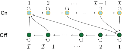
Figure 4: State transition diagram for pool pump model.

In this paper we take the same state space, but with a different interpretation of each state: Here as in [5] we employ geometric sampling, so that the nominal state transition matrix is of the form (24). The state transition diagram for $P_{0}$ is shown in Figf:ppp.

In the experiments that follow, the transition matrix $S_{0}$ is the model with 12-hour cleaning cycle from [4], in which ${\cal I}=48$, and hence $d=|{\sf X}|=96$. It is assumed that the BA sends a signal every five minutes, and that the geometric sampling parameter is $\gamma=1/6$. Consequently, the state of each load changes every 30 minutes on average.

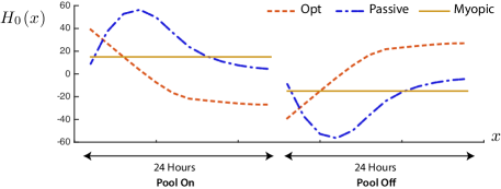
Figure 5: $H_{0}={\cal H}(P_{0})$ in three designs for the pool pump model.

There is no need to model uncertainty from nature. Hence the function $H={\cal H}(P)$ will depend only on its second variable: $H(x,x^{\prime})=H(x^{\prime})$ for all $(x,x^{\prime})$.

In each of these experiments the nominal transition matrix $P_{0}$ was taken as an input to the algorithm, and not $S_{0}$. The resulting transition matrix $P_{\zeta}$ is of the form given in (25), in which the sampling rate is state-dependent for non-zero $\zeta$. For the SPD solution it was necessary to use $P_{0}$ as the input: It can be shown that the transition matrix $P^{\triangledown}_{0}$ is irreducible, but $S^{\triangledown}_{0}\mathbin{:=}S_{0}^{\Lsh}S_{0}$ is not irreducible in this example. Recall from Theorem 2.3 that irreducibility is required to ensure the existence of the SPD solution.

Fig. 5 shows the function $H_{0}={\cal H}(P_{0})$ obtained in three sets of experiments. The normalization in the myopic design uses $H_{0}=30(\mathchoice{\mbox{\small$\cal U$}}{\mbox{\small$\cal U$}}{\mbox{$\scriptstyle\cal U$}}{\mbox{$\scriptscriptstyle\cal U$}}-1/2)$. This is equivalent to using $\cal U$ since adding a constant does not impact $R_{\zeta}$, and the multiplication by $30$ only scales $\zeta$. A comparison of the three transfer functions $G^{+}$ obtained through a linearization at $\zeta=0$ is shown in Fig. 6. The myopic design appears to be preferable to the two others: in particular, the phase plot stays nearest to zero in this design.

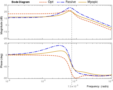
Figure 6: Bode plots obtained from three designs for the pool pump model.

One drawback with the myopic design is that we have no basis for analysis. Difficulties are also observed in numerical experiments if we allow $|\zeta|$ to take on values far from zero. Of the three designs, the IPD is found to be the most numerically stable in all of the experiments considered, in the sense that the dynamics change predictably with $\zeta$, and the linearization about each value of $\zeta$ are nearly the same for a large range of $\zeta$.

In the next subsection we move to a different class of loads in which we cannot ignore exogenous randomness. We consider in greater depth the difference between the myopic and IPD outcomes for a wider range of $\zeta$. It is found again that the two designs are very similar locally (for $\zeta\sim 0$), but the myopic design is numerically unstable for $\zeta$ outside of a small neighborhood of the origin.

4.2 Thermostatically controlled loads

A thermostatically controlled load (TCL) such as a water heater, refrigerator, or air-conditioner is a device for which temperature control is achieved using a dead-band. It is assumed here that power consumption takes just two values (on or off). To simplify discussion, attention is directed to a cooling device, such as a residential refrigerator.

We begin with a noise free model, described as the controlled linear system,

$$\Theta(k+1)=\Theta(k)+(1-\varrho)(\Theta_{a}-\Theta(k)-m(k)\Theta_{g}),$$ (35)

where $m(k)=1$ or $0$ indicates if the unit is on or off, $\Theta_{a}$ is ambient temperature, $\varrho$ depends on the dynamics of the load, and $\Theta_{g}$ the depends on the physics of the device. One example considered in [15] is an air conditioner for which $\Theta_{g}=R\text{$P_{\text{trans}}$}=2\times 14=28$ (this and other parameters are summarized in Table 1).

A signal from the BA is broadcast at 20 second intervals. The parameter $\varrho$ is obtained based on this sampling time, and the product of thermal resistance and capacitance: $\varrho=\exp[-20/(RC)]$, with $RC$ also in units of seconds. The value $RC=4$ obtained from Table 1 is in units of hours — on scaling to seconds we obtain,

$$\varrho=e^{-h/(RC)}=e^{-20/(4\times 60^{2})}=e^{-1/720}\approx 1-1/720$$

Parameter	Meaning	Value
$\Theta_{\text{set}}$	set temperature set-point	$20^{\circ}$C
$[\text{$\Theta_{\text{min}}$},\text{$\Theta_{\text{max}}$}]$	temperature dead-band	$20\pm 0.5{}^{\circ}$C
$\Theta_{a}$	ambient temperature	32∘C
$R$	thermal resistance	2∘C/kW
$C$	thermal capacitance	2 kWh/∘C
$P_{\text{trans}}$	energy transfer rate	14 kW

Table 1: Homogeneous air conditioner parameters — mean data from Table 4.1 of [15].

This model is based on the physics of heating and cooling, but the dynamics are accurately captured by a constant drift model:

$$\Theta(k+1)=\Theta(k)-m(k)\delta_{-}+(1-m(k))\delta_{+}$$ (36)

With drift parameters $\delta_{\pm}$ carefully chosen, the behavior of the two models is barely distinguishable.

The deterministic model (36) is the basis of a stochastic model,

$$\Theta(k+1)=\Theta(k)-m(k)\delta_{-}+(1-m(k))\delta_{+}+\Delta(k+1)$$ (37)

in which $\Delta$ is a zero-mean, i.i.d.  sequence. In the experiments that follow the sampling time was taken to be $2$ seconds, and $\Delta$ was taken to be Gaussian with variance $10^{-6}$ (the small variance is justified with this fast sampling rate).

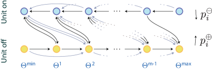
Figure 7: State transition diagram for a TCL providing cooling.

A Markov chain model can be constructed with state $X(k)=(m(k),X_{n}(k))$ evolving on ${\sf X}={\sf X}_{\sf u}\times{\sf X}_{\sf n}$, where $X_{n}(k)=\Theta(k)$ and ${\sf X}_{\sf u}=\{\ominus,\oplus\}$; the interpretation is the same as in the pool filtration model, with the interpretation $m(k)=\oplus$ is the same as $m(k)=1$ in (37). Temperatures are restricted to a lattice to obtain a finite state-space Markov chain. To obtain $d$ states, assume that $d\geq 4$ is an even number, and discretize the interval $[\text{$\Theta_{\text{min}}$},\text{$\Theta_{\text{max}}$}]$ into $d/2$ values as follows: ${\sf X}_{\sf n}=\{\text{$\Theta_{\text{min}}$}+kT_{\Delta}:0\leq k\leq d/2-1\}$, in which the increments in the lattice are $T_{\Delta}=(\text{$\Theta_{\text{max}}$}-\text{$\Theta_{\text{min}}$})/(d/2-1)$.

A nominal randomized policy for $m$ defines the transition matrix $R_{0}$. Following the notation of [4], the nominal transition matrix for $m$ is defined by

$$R_{0}(x,\oplus) =\begin{cases}1-p^{\ominus}(x_{n})&x=(\oplus,x_{n})\\ p^{\oplus}(x_{n})&x=(\ominus,x_{n})\end{cases}$$ (38)

$$R_{0}(x,\ominus) =\begin{cases}p^{\ominus}(x_{n})&x=(\oplus,x_{n})\\ 1-p^{\oplus}(x_{n})&x=(\ominus,x_{n})\end{cases}$$

As in [4], the definition of $p^{\ominus}$ is based on the specification of a cumulative distribution function $F^{\ominus}$ defined on the interval $[\text{$\Theta_{\text{min}}$},\text{$\Theta_{\text{max}}$}]$. This CDF is meant to model the statistics of the time interval during which the unit is off, for the model with continuous state space. We define $p^{\ominus}(x_{n})=1$ for $x_{n}=\text{$\Theta_{\text{max}}$}$, $p^{\ominus}(x_{n})=F^{\ominus}(x_{n})$ for $x_{n}=\text{$\Theta_{\text{min}}$}$, and for all other values,

$$p^{\ominus}(x_{n})=[F^{\ominus}(x_{n})-F^{\ominus}(x_{n}-T_{\Delta})]/[1-F^{\ominus}(x_{n}-T_{\Delta})]$$

In the experiments that follow, the general form taken for $F^{\ominus}$ was chosen in the parameterized family,

$$F^{\ominus}(x_{n})=\exp(-(\text{$\Theta_{\text{max}}$}-x_{n})^{\rho}/(2\sigma^{\rho})),\ \text{$\Theta_{\text{min}}$}\leq x_{n}\leq\text{$\Theta_{\text{max}}$},$$

with $\sigma,\rho>0$. The values $T_{\Delta}=0.05$, $\sigma=0.02$ and $\rho=0.75$ were used for $p^{\ominus}$ and $p^{\oplus}$ in the experiments surveyed here.

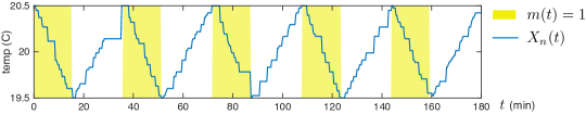
Figure 8: Trajectory of TCL model with geometric sampling $\gamma=1/3$.

In addition, geometric sampling was applied: a family of models of the form (26) was constructed, in which $R_{0}$ was used to define $S_{0}$ in (24). The construction of a model of this form requires a different interpretation of the nature component of the state ${\mathchoice{\mbox{\boldmath$X$}}{\mbox{\boldmath$X$}}{\mbox{\boldmath$\scriptstyle X$}}{\mbox{\boldmath$\scriptscriptstyle X$}}}_{n}$.

To obtain dynamics of the form (24), let $\{\tau_{k}\}$ denote the discrete renewal process in which $\tau_{0}=0$ and $\{\Delta_{k}=\tau_{k}-\tau_{k-1}:k\geq 1\}$ is i.i.d., with a geometric marginal:

$${\sf P}\{\Delta_{k}>n\}=\gamma^{n},\qquad n\geq 0,\ k\geq 1.$$

The nature component of the state is constant on each discrete-time interval $(t:\tau_{k}\leq t<\tau_{k+1})$, with $X_{n}(t)=\Theta(\tau_{k})$ on this interval. Given a nominal randomized policy for the input process ${\mathchoice{\mbox{\boldmath$X$}}{\mbox{\boldmath$X$}}{\mbox{\boldmath$\scriptstyle X$}}{\mbox{\boldmath$\scriptscriptstyle X$}}}_{u}={\mathchoice{\mbox{\boldmath$m$}}{\mbox{\boldmath$m$}}{\mbox{\boldmath$\scriptstyle m$}}{\mbox{\boldmath$\scriptscriptstyle m$}}}$, the nominal transition matrix $Q_{0}$ can be estimated via Monte-Carlo based on a simulation of (37), or from measurements of an actual TCL.

A Markov model with this transition matrix would also require $m(t)$ constant on each of the intervals $(t:\tau_{k}\leq t<\tau_{k+1})$, $k\geq 0$. In simulations this constraint was violated occasionally since $m(t)=1$ when $\Theta(t)>\text{$\Theta_{\text{max}}$}$, and $m(t)=0$ when $\Theta(t)<\text{$\Theta_{\text{min}}$}$. This leads to modeling error that is small, provided $\gamma$ is not too close to unity. Fig. 8 shows an example of the evolution of ${\mathchoice{\mbox{\boldmath$X$}}{\mbox{\boldmath$X$}}{\mbox{\boldmath$\scriptstyle X$}}{\mbox{\boldmath$\scriptscriptstyle X$}}}_{n}$ with $\gamma=1/3$. The temperature never violates the dead-band constraint because of the constraints imposed on ${\mathchoice{\mbox{\boldmath$X$}}{\mbox{\boldmath$X$}}{\mbox{\boldmath$\scriptstyle X$}}{\mbox{\boldmath$\scriptscriptstyle X$}}}_{u}$.

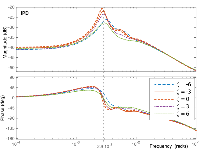
(a) IPD Design

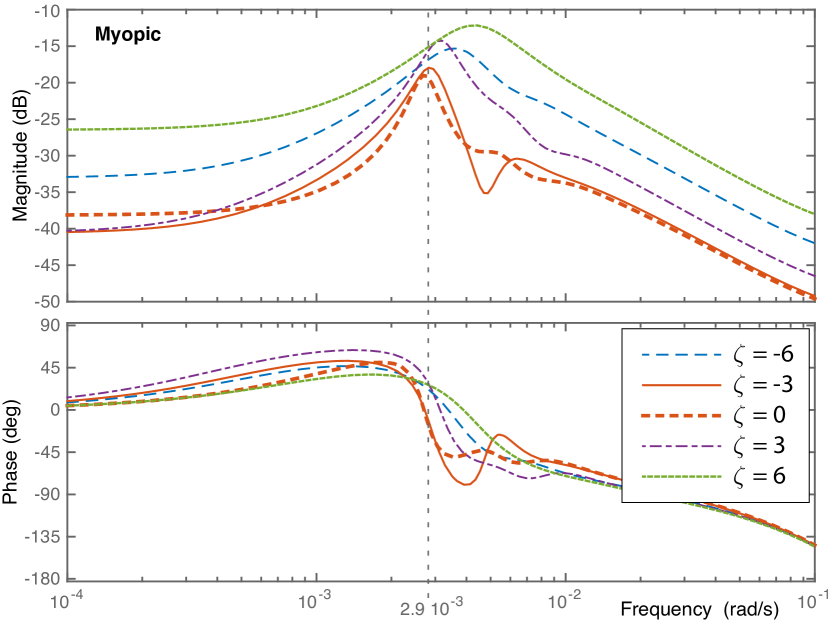
(b) Myopic Design

Figure 9: Bode plots for two designs, based on linearizations at five values of $\zeta$. Bode plots for the myopic design are less reliable for $|\zeta|>3$.

In this example the transition matrix $S^{\triangledown}_{0}\mathbin{:=}S_{0}^{\Lsh}S_{0}$ is irreducible, so that the SPD solution is computable. Because of exogenous randomness, there is no motivation for this approach: Theorem 2.3 guarantees a passive linearization only when $P_{0}=R_{0}$. Moreover, numerical results using this method were not encouraging: The resulting family of transition matrices $\{P_{\zeta}\}$ is extremely sensitive to $\zeta$.

The linearization about $\zeta=0$ for the myopic design was similar to the IPD solution, but as seen in Figs. 9(a) and 9(b), the behaviors quickly diverge for values beyond $|\zeta|=3$.

In conclusion, although the transfer functions for the linearizations at $\zeta=0$ are nearly identical, in the myopic design the input-output behavior is unpredictable for $|\zeta|>3$. The input-output behavior for IPD is much closer to a linear system for a wider range of $\zeta$. This is consistent with results from prior research [4, 2, 5].

5 Conclusions

This paper has developed new approaches to distributed control for demand dispatch. There is much more work to do on algorithm design, and large-scale testing.

References

- [1] P. Barooah, A. Bušić, and S. Meyn, “Spectral decomposition of demand-side flexibility for reliable ancillary services in a smart grid,” in Proc. 48th Annual Hawaii International Conference on System Sciences (HICSS), Kauai, Hawaii, 2015, pp. 2700–2709.
- [2] Y. Chen, A. Bušić, and S. Meyn, “Individual risk in mean-field control models for decentralized control, with application to automated demand response,” in Proc. of the 53rd IEEE Conference on Decision and Control, Dec. 2014, pp. 6425–6432.
- [3] H. Hao, Y. Lin, A. Kowli, P. Barooah, and S. Meyn, “Ancillary service to the grid through control of fans in commercial building HVAC systems,” IEEE Trans. on Smart Grid, vol. 5, no. 4, pp. 2066–2074, July 2014.
- [4] S. Meyn, P. Barooah, A. Bušić, Y. Chen, and J. Ehren, “Ancillary service to the grid using intelligent deferrable loads,” IEEE Trans. Automat. Control, vol. 60, no. 11, pp. 2847–2862, Nov 2015.
- [5] Y. Chen, A. Bušić, and S. Meyn, “State estimation for the individual and the population in mean field control with application to demand dispatch,” CoRR and to appear, IEEE Transactions on Auto. Control, 2015. [Online]. Available: http://arxiv.org/abs/1504.00088v1
- [6] S. Meyn, P. Barooah, A. Bušić, and J. Ehren, “Ancillary service to the grid from deferrable loads: The case for intelligent pool pumps in Florida,” in Proceedings of the 52nd IEEE Conf. on Decision and Control, Dec 2013, pp. 6946–6953.
- [7] J. Mathieu, S. Koch, and D. Callaway, “State estimation and control of electric loads to manage real-time energy imbalance,” IEEE Trans. Power Systems, vol. 28, no. 1, pp. 430–440, 2013.
- [8] B. Sanandaji, H. Hao, and K. Poolla, “Fast regulation service provision via aggregation of thermostatically controlled loads,” in 47th Hawaii International Conference on System Sciences (HICSS), Jan 2014, pp. 2388–2397.
- [9] B. Biegel, L. Hansen, P. Andersen, and J. Stoustrup, “Primary control by ON/OFF demand-side devices,” IEEE Trans. on Smart Grid, vol. 4, no. 4, pp. 2061–2071, Dec 2013.
- [10] A. Bušić and S. Meyn, “Passive dynamics in mean field control,” in Proc. 53rd IEEE Conference on Decision and Control, Dec 2014, pp. 2716–2721.
- [11] E. Todorov, “Linearly-solvable Markov decision problems,” in Advances in Neural Information Processing Systems 19, B. Schölkopf, J. Platt, and T. Hoffman, Eds. Cambridge, MA: MIT Press, 2007, pp. 1369–1376.
- [12] P. Guan, M. Raginsky, and R. Willett, “Online Markov decision processes with Kullback-Leibler control cost,” IEEE Trans. Automat. Control, vol. 59, no. 6, pp. 1423–1438, June 2014.
- [13] S. P. Meyn and R. L. Tweedie, Markov chains and stochastic stability, 2nd ed. Cambridge: Cambridge University Press, 2009, published in the Cambridge Mathematical Library. 1993 edition online.
- [14] A. Bušić and S. Meyn, “Respecting nature and nurture in Markov Decision Processes with Kullback–Leibler control cost,” 2015, In preparation.
- [15] J. Mathieu, “Modeling, analysis, and control of demand response resources,” Ph.D. dissertation, University of California at Berkeley, 2012.