Covariantized Matrix theory for D-particles

Abstract:

We reformulate the Matrix theory of D-particles in a manifestly Lorentz-covariant fashion in the sense of 11 dimesnional flat Minkowski space-time, from the viewpoint of the so-called DLCQ interpretation of the light-front Matrix theory. The theory is characterized by various symmetry properties including higher gauge symmetries, which contain the usual SU($N$) symmetry as a special case and are extended from the structure naturally appearing in association with a discretized version of Nambu’s 3-bracket. The theory is scale invariant, and the emergence of the 11 dimensional gravitational length, or M-theory scale, is interpreted as a consequence of a breaking of the scaling symmetry through a super-selection rule. In the light-front gauge with the DLCQ compactification of 11 dimensions, the theory reduces to the usual light-front formulation. In the time-like gauge with the ordinary M-theory spatial compactification, it reduces to a non-Abelian Born-Infeld-like theory, which in the limit of large $N$ becomes equivalent with the original BFSS theory.

1 Introduction

From the viewpoint of exploring non-perturbative formulations of string theory, the conjecture of 11 dimensional M-theory occupies a special pivotal position in providing a candidate for the strong-coupling limit of the type IIA (and $E_{8}\times E_{8}$ Heterotic) string theory. Let us first recall the basic tenets of M-theory conjecture: The background space-time is (10,1) space-times instead of (9,1) space-times of string theory. The 10-th spatial dimension is compactified, $x^{10}\sim x^{10}+2\pi R_{11}$, around a circle of radius $R_{11}=g_{s}\ell_{s}$, with $g_{s}$ and $\ell_{s}$ being the string coupling of type IIA superstrings and fundamental string-length constant, respectively. The gravitational scale $\ell_{11}$ in 11 dimensions as the sole length scale of M-theory is related to these string-theory constants by $\ell_{11}=g_{s}^{1/3}\ell_{s}$, so that the theory with a finite gravitational length in infinitely ($R_{11}\rightarrow\infty$) extended 11 dimensional space-times corresponds to a peculiar limit of string theory characterized by $g_{s}\rightarrow\infty$ and $\ell_{s}^{2}=\ell_{11}^{3}/R_{11}\rightarrow 0$. In particular, the gravitational interactions at long distance scales much larger than $\ell_{11}$ are expected to be described by the classical theory of 11 dimensional supergravity. Dynamical degrees of freedom corresponding to strings are expected to be (super) membranes (or M2-branes): super membranes wrapped once around the compactified circle are supposed to behave as fundamental strings in the remaining 10 dimensional space-time in the limit $g_{s}\rightarrow 0$ with finite $\ell_{s}$. Various D-brane (and other) excitations of string theory also find their roles naturally. For instance, D0-branes, namely D-particles, are special Kaluza-Klein excitations of 11 dimensional gravitons with the single quantized unit $p_{10}=1/R_{11}$ of momentum along the circle in the 11th dimension. D2-branes are super-membranes lying entirely in un-compactified 10 dimensional space-times, and D4-branes are wrapped M5-branes which are 5-dimensionally extended objects, being dual to M2-branes in the sense of electromagnetic duality of Dirac with respect to RR gauge fields, and so on.

In spite of various circumstantial evidence for this remarkable conjecture, only known and perhaps practically workable example of concrete formulations of M-theory is the so-called BFSS M(atrix) theory [1]. This proposal was originated from a coincidence of effective theories for two apparently differenct objects, namely, D-particles and supermembranes. In the limit of small $\ell_{s}$, the effective low-energy theory [2] for many-body dynamics of D-particles is supersymmetric SU($N$) Yang-Mills quantum mechanics which is obtained from the maximally supersymmetric super Yang-Mills theory in 10 dimensions by dimensional reduction of the base (9,1) space-time to (0,1) world line, in which 9 spatial components of gauge fields turn into matrix coordinates as collective variables representing motion (diagonal matrix elements) and interaction (off-diagonal matrix elements) of D-particles in terms of short open strings. Essentially the same super Yang-Mills quantum mechanics also appears [3] as a possible regularization of a single super membrane formulated in the light-front quantization, approximating to a super membrane in an appropriate limit of large $N$. In the latter case, the functional space of membrane coordinates defined on two-dimensional spatial parameter space of the membrane world-volume is replaced by the ring of Hermitian $N\times N$ matrices. The crux of the proposal was to realize that, by uniting these two seemingly different interpretations as effective theories, the super Yang-Mills matrix model may hopefully provide not only a regularization of a single membrane, but more importantly would describe also “partons” for membranes and in principle all other excitations of M-theory in a more fundamental manner.

Suppose we consider the situation where all of constituent partons have a unit 10-th momentum $p_{10}=1/R_{11}$ of the same sign (namely, no anti-D-paricles) along the compactified circle, the total 10-th momentum of a system consisting of $N$ partons is $P_{10}=N/R_{11}=Np_{10}$. In the limit of large $N$, it defines an infinite momentum frame $P_{10}\rightarrow\infty$ along the compactifed circle. Then the coincidence between the effective non-relativistic Yang-Mills quantum mechanics of D-branes and the light-front regularization of supermembrane is understandable. Remember the case of a single relativistic particle with mass-shell condition $P^{\mu}P_{\mu}+m^{2}=0$,

$$-P^{-}\equiv P^{0}-P^{10}=\sqrt{(P^{i})^{2}+m^{2}+(P^{10})^{2}}-P^{10}\rightarrow\frac{(P^{i})^{2}+m^{2}}{2P^{10}}$$ (1)

with the indices $i=1,2,\ldots,9$ running only over transverse directions. By making identification $P^{10}=N/R_{11}$ for the compactified 10-th direction, we expect that this form of $P^{0}$ corresponds to the center-of-mass energy of an $N$ D-particle system, providing that $m^{2}$ is the effective relativistically invariant squared mass of the system. We can also adopt an alternative viewpoint, namely the so-called DLCQ (discrete light-cone quantization) interpretation: instead of 10-th spatial direction, we can assume [4] that a light-like direction $x^{-}\equiv x^{10}-x^{0}$ is compactified into a circle of radius $R$ with periodicity $x^{-}\sim x^{-}+2\pi R$. Then the light-like momentum $P^{+}\equiv P^{10}+P^{0}$ is discretized, $P^{+}/2=N/R$. With the same proviso for $N$ again as the size of matrices, we have the same expression as (1) now as an exact relation without taking the large $N$ limit

$$-P^{-}=\frac{(P^{i})^{2}+m^{2}}{P^{+}}=R\frac{(P^{i})^{2}+m^{2}}{2N},$$ (2)

but with $R_{11}$ being replaced by $R$.

The difference of these two interpretations lies in the natures of Lorentz symmetry in 11 dimensions. In the former spatial compactification scheme, a boost along the compactified 10-th direction is a discrete change of the quantum number $N$ with fixed (and hence Lorentz invariant) $R_{11}$, while in the latter that is nothing but a continuous rescaling of $R$ with fixed $N$. Thus, in the DLCQ interpretation, $N$ is Lorentz-invariant and $P^{+}$ is a continuously varying dynamical variable. In both cases, however, the limit of un-compactification (namely, strong-coupling limit of type IIA string theory) requires the large $N$ limit, because in the DLCQ case the longitudinal momentum $P^{+}$ must also become a continuous finite variable even in a fixed Lorentz frame which is possible only by allowing infinite $R$ and $N$. Further arguments [5] justifying the viewpoint of the DLCQ interpretation were given, suggesting that it could be understood as a result of taking a limit of large boost from the former interpretation with small spatial compactification radius corresponding to a limit of weak string coupling. In both cases, the parton interpretation of D-particles requires that possible KK excitations with multiple units of momenta, such as $p_{10}=2/R_{11}$ or $p^{+}=4/R$ and higher, are interpreted as composite states of two and higher numbers of partons.

It is also to be noted that the theory naturally describes general multi-body states of these composite states, since $N\times N$ matrices contain as subsystems block-diagonal matrices $N_{i}\times N_{i}$ with $N=\sum_{i}N_{i}$. The off-diagonal blocks then are responsible for interactions of these subsystems. Therefore, it is essential to treat systems with all different $N$’s from $N=2$ to infinity on an equal footing, even apart from the requirement of including all possible values of the total longitudinal momentum. Note also that the exchanges of longitudinal momentum $p_{10}$ or $p^{+}$ among constituent subsystems occur in principle as (non-perturbative) processes of rearranging constituent partons in the internal dynamics of SU($N$) Yang-Mills (super) quantum mechanics.

From the late 1990s to the early 2000s, numerous works testing the proposal appeared. In particular, the DLCQ interpretation made us possible to perform certain perturbative analyses of super Yang-Mills quantum mechanics in exploring whether it gives reasonable gravitational interactions of D-particles and other excitations with respect to scatterings of those excitations in reduced 10 dimensional space-time. Although we had various encouraging results supporting the M(atrix) theory conjecture, the final conclusion has not been reached yet.

One of the problems left was whether and how fully Lorentz covariant formulations of the theory would be possible. If we adopt the viewpoint of the DLCQ interpretation supposing that the Matrix theory with finite $N$ already gives an exact theory with special light-like compactification, it is not unreasonable to believe the existence of covariant version of the finite $N$ super Yang-Mills mechanics. This is particularly so, if we recall that the above relation between the discretized light-like momentum and the size of matrices still allows continuously varying $P^{+}$ with an arbitrary (real and positive) parameter $R$ corresponding to boost transformations. Since $N$ is invariant under boost by definition in the DLCQ interpretation, it seems natural to imagine a generalization of super Yang-Mills mechanics with full covariance allowing general Lorentz transformations for fixed finite $N$ as a conserved quantum number, not restricted only to boost transformation along the compactified circle, with all of the 10+1 directions of eleven dimensional Minkowski space-time being treated equally as matrices or some extensions of matrices. Otherwise, it seems difficult to justify the DLCQ interpretation. If such a covariant theory exists as in the case of the ordinary particle mechanics, the DLCQ matrix theory would be obtained as an exact theory from a covariantized Matrix theory with a Lorentz-invariant effective mass square. Although we have to take the limit of large $N$ to elevate it to a full fledged formulation of M-theory, a consistent covariant formulation with finite $N$ could be an intermediate step toward our ultimate objective.

With this motivation in mind, we studied in ref. [9] the quantization (or more precisely discretization) of the Nambu bracket [10]. The Nambu (-Poisson) bracket naturally appears in covariant treatments of classical membranes. For instance, the bosonic action of a membrane can be expressed in the form

$$A_{{\rm mem}}=-\frac{1}{\ell_{11}^{3}}\int d^{3}\xi\Bigl{(}\frac{1}{e}\{X^{\mu},X^{\nu},X^{\sigma}\}_{{\rm N}}\{X_{\mu},X_{\nu},X_{\sigma}\}_{{\rm N}}-e\Bigr{)},$$ (3)

$$\{X^{\mu},X^{\nu},X^{\sigma}\}_{{\rm N}}\equiv\sum_{a,b,c}\epsilon^{abc}\partial_{a}X^{\mu}\partial_{b}X^{\nu}\partial_{c}X^{\sigma},$$ (4)

giving the Dirac-Nambu-Goto form when the auxiliary variable $e$ is eliminated. Note that $\xi^{a}$ $(a,b,c\in(1,2,0))$ parametrize the 3 dimensional world volume of a single membrane, and space-time indices $\mu,\nu,\ldots$ run over 11 directions of the target space-time. This is analogous to the treatments of strings where Poisson bracket plays a similar role [11].

In ref. [9] we proposed two possibilities of quantization: one was to use the ordinary square matrices and their commutators, and the other was more radically to introduce new objects, cubic matrices with three indices. A natural idea seemed to regularize the above action (3) directly by replacing the NP bracket by a finitely discretized version and the integral over the world volume by an appropriate “Trace” operation in the algebra of quantized coordinates corresponding to classical coordinates $X^{\mu}(\xi)$. The usual light-front action should appear as a result of an appropriate gauge fixing of a higher gauge symmetry which generalizes its continuous counterpart, the area-preserving diffeomorphism transformations formulated a la Nambu’s mechanics

$$\delta X^{\mu}=\{F,G,X^{\mu}\}_{{\rm N}},$$ (5)

with $(F(\xi),G(\xi))$ being two independent local gauge parameter-functions. At that time, we could not accomplish this program. One of the stumbling blocks was our tacit demand that the light-front time coordinate should also emerge automatically in the process of gauge fixing. This seemed to be necessary because (4) involves a time derivative.

In the present work, we reconsider the program of the covariantization of M(atrix) theory. However, we do not pursue the above mentioned analogy with the theory of super membrane too far. In particular, we do not assume the above relation between the membrane action and Nambu bracket. Such an analogy does not seem to be essential from the viewpoint of the DLCQ interpretation with finite $N$, since this analogy suggests the covariance could only be recovered in a large $N$ limit. We use Nambu-type transformations only as a convenient tool to motivate higher gauge symmetries which would be necessarily required for achieving manifest covariance using 11 dimensional matrix variables: an appropriate gauge-fixing of such higher gauge symmetries would lead us to the usual light-front theory with 9 dimensional matrix variables.

With regards to the problem of the emergence of time parameter describing the causal dynamics of matrices, we reset our goal at a lower level. Namely, we introduce from the outset a single Lorentz invariant (proper) time parameter $\tau$ together with an “ein-bein” auxiliary variable $e(\tau)$, which transforms as $d\tau e(\tau)=d\tau^{\prime}e^{\prime}(\tau^{\prime})$ under an arbitrary re-parametrization $\tau\rightarrow\tau^{\prime}$ and generates the mass-shell condition for the center-of-mass variables with an effective mass-square operator. Thus the proper-time is essentially associated with the trajectory of the center-of-mass. From the viewpoint of relativistically covariant formulation of many-body systems in the configuration-space picture, as opposed to the usual second-quantized-field theory picture, we would expect that the proper time-parameter should be associated independently with each particle degree of freedom, since we have to impose mass-shell conditions separately to each particle. This is possible in the usual relativistic quantum mechanics where we can separately treat particle degrees of freedom and field degrees of freedom which mediate interactions among particles, especially using Dirac’s interaction representation. However, in matrix models such as super Yang-Mills quantum mechanics, such a separation is not feasible, since the SU($N$) gauge symmetry associated with matrices requires us to treat the coordinate degrees and interaction degrees of freedom embedded together in each matrix inextricably as a single entity. In fact, in either case of M-theory compactifications formulated by the super Yang-Mills quantum mechanics, there is no trace of such mass-shell conditions set independently for each constituent parton. In our approach, the time parameters (not physical time components) of all the dynamical degrees of freedom are by definition synchronized globally to a single invariant Lorentz-invariant parameter of the center-of-mass degrees of freedom. Under this circumstance, we extend a higher gauge symmetry exhibited in our version of quantized Nambu bracket, and argue that it can lead to a mechanism for formulating many-body systems covariantly in a configuration-space formalism without negative metric, replacing methods with many independent proper-time parameters, and hopefully characterizing the peculiar general-relativisitic nature of D-particles as partons of M-theory.

In section 2, we first reformulate, with some slight extensions, our old proposal for a discretized Nambu bracket using matrix commutators in terms of ordinary square matrices to motivate higher gauge symmetries, and introduce a covariant canonical formalism to develop higher gauge transformations. In section 3, we present the bosonic part of our action. We discuss various symmetry properties of the action and their implications. In particular, it will be demonstrated that our theory reduces to the usual formulation of Matrix theory in a light-front gauge. In section 4, we extend our theory minimally to a supersymmetric theory, with some details being relegated to two appendices. In section 5, we summarize our work and conclude by mentioning various future possibilities and confronting problems.

2 Canonical formalism of higher gauge symmetries

In the present and next sections, for the purpose of elucidating the basic ideas and formalisms step by step in a simple setting without complications of fermionic degrees of freedom, we restrict ourselves to bosonic variables. Extension to including fermionic variables in a supersymmetric fashion will be discussed later.

In the first part, we start from briefly recapitulating our old proposal for a discretized version of the Nambu bracket in the matrix form as a motivation toward higher gauge symmetries, and then in the sequel we will extend further and complete the higher gauge symmetries in the framework of a first-order canonical formalism in a relativistically covariant fashion.

2.1 From a discretized Nambu 3-bracket to a higher gauge symmetry

Let us denote $N\times N$ hermitian matrix variables using slanted boldface symbol, like $\bm{X},\bm{Y},\bm{Z},\cdots$, and introduce non-matrix variables associated with them and denoted by a special subscript M, like $X_{{\rm{\tiny M}}},Y_{{\rm{\tiny M}}},Z_{{\rm{\tiny M}}},\cdots$. All these variables are functions of the invariant time parameter $\tau$ and assumed to be scalar with respect to its re-parameterization. When we deal with matrix elements explicitly, we designate them by $X_{ab},\ldots$ without boldface symbol. Originally in ref. [9] we identified the $X_{{\rm{\tiny M}}}$’s to be the traces of the corresponding matrices. But that is not necessary, and in the present work we treat them as new independent dynamical degrees of freedom. This is the price we have to pay to realize a higher gauge symmetry, but we will have a reward too. Treating them as a pair of non-matrix and matrix variables, we denote like $X=(X_{{\rm M}},\bm{X})$ for notational brevity.

The discretized NP bracket, which we simply call 3-bracket, is then defined as

$$[X,Y,Z]\equiv(0,X_{{\rm{\tiny M}}}[\bm{Y},\bm{Z}]+Y_{{\rm{\tiny M}}}[\bm{Z},\bm{X}]+Z_{{\rm{\tiny M}}}[\bm{X},\bm{Y}]).$$ (6)

Note that the M-component of $[X,Y,Z]$ is zero by definition. This is totally skew-symmetric and satisfies the so-called Fundamental Identity (FI) essentially as a consequence of the usual Jacobi identity,

$$[F,G,[X,Y,Z]]=[[F,G,X],Y,Z]+[X,[F,G,Y],Z]+[X,Y,[F,G,Z]].$$ (7)

The proof given in ref. [9], to which we refer readers for further details and relevant literature related to this identity, goes through as it stands for our slightly extended cases too. In particular, the absence ($[X,Y,Z]_{{\rm M}}=0$) of the M-component for the 3-bracket follows from the property that, for the matrix part of the right-hand side of (7), the contributions involving the commutator $[\bm{F},\bm{G}]$ cancel out among themselves without performing any trace operations for arbitrary sef of three elements $(X,Y,Z)$, guaranteeing the absence of the term $[X,Y,Z]_{{\rm M}}[\bm{F},\bm{G}]$. The latter would correspond to the last term in the matrix part of (6) and, if non-vanishing, contradict the vanishing of $[X,Y,Z]_{{\rm M}}$ on the left-hand side of the FI.

If we interpret the bracket $[F,G,X]$ for arbitrary variable $X$ as an infinitesimal gauge transformation with generators $F$ and $G$, which are local with respect to the proper time $\tau$,

$$\delta X \equiv i[F,G,X]=(0,i[F_{{\rm{\tiny M}}}\bm{G}-G_{{\rm{\tiny M}}}\bm{F},\bm{X}]+i[\bm{F},\bm{G}]X_{{\rm{\tiny M}}})$$ (8)

as a generalization of (5), the FI is nothing but the distribution law of gauge transformations for 3-bracket. Without losing generality, we define that the gauge-parameter matrix functions $\bm{F}$ and $\bm{G}$ are both traceless. An important characteristic property [9] of this gauge transformation is that it enables us to gauge away the traceless part of one of the matrix variables whenever its ${\rm{\tiny M}}$ component is not zero, due to the second term in (8). On the other hand, it should be kept in mind that both the trace-part of the matrices and $X_{{\rm{\tiny M}}}$ are inert (${\rm Tr}(\delta\bm{X})=0=\delta X_{{\rm{\tiny M}}}$ ) against the gauge transformations (8). We will later extend the gauge transformation slightly such that the center-of-mass coordinate (but still not for $X_{{\rm{\tiny M}}}$) is also subject to extended gauge transformations.

Actually, it is useful to generalize the above gauge transformation to

$$\delta X=i\sum_{r}[F^{r},G^{r},X]=\bigl{(}0,\sum_{r}i[F_{{\rm M}}^{r}\bm{G}^{r}-G_{{\rm M}}^{r}\bm{F}^{r},\bm{X}]+i\sum_{r}[\bm{F}^{r},\bm{G}^{r}]X_{{\rm M}}\bigr{)}$$ (9)

by introducing an arbitrary number of independent gauge functions discriminated by indices $r=1,2,\ldots$. Since the FI (7) is satisfied for each $r$ separately, it is still valid after summing over them. This means that two traceless Hermitian matrices,

$$\bm{H} \equiv\sum_{r}F_{{\rm M}}^{r}\bm{G}^{r}-G_{{\rm M}}^{r}\bm{F}^{r},$$ (10)

$$\bm{L} \equiv i\sum_{r}[\bm{F}^{r},\bm{G}^{r}],$$ (11)

can be regarded as being completely independent to each other. In what follows, we adopt this generalized form of gauge transformation,

$$\delta_{HL}X\equiv\delta_{H}X+\delta_{L}X=(0,i[\bm{H},\bm{X}]+\bm{L}X_{{\rm M}}),$$ (12)

with an obvious decomposition into $\delta_{H}$ and $\delta_{L}$. The 3-bracket form of gauge transformation itself does not play any essential role for our development from this point on, though the 3-bracket notation will still be convenient symbolically in expressing action in a compact form.

For any pair of two matrices $\bm{X},\bm{Y}$ with vanishing M-components $X_{{\rm{\tiny M}}}=0=Y_{{\rm{\tiny M}}}$, the trace of their bilinear product

$$\langle X,Y\rangle\equiv{\rm Tr}(\bm{X}\bm{Y})$$ (13)

is invariant under the gauge transformation, because the gauge transformation then reduces to a usual SU($N$) transformation $\delta_{HL}\bm{X}=i[\bm{H},\bm{X}]$ and $\delta_{HL}\bm{Y}=i[\bm{H},\bm{Y}]$ and hence satisfies a derivation property $(\delta_{HL}\bm{X})\bm{Y}+\bm{X}(\delta_{HL}\bm{Y})=i[\bm{H},\bm{X}\bm{Y}]$:

$$\delta_{HL}\langle X,Y\rangle\equiv\langle\delta_{HL}X,Y\rangle+\langle X,\delta_{HL}Y\rangle=0.$$ (14)

Unlike [9], this is valid irrespectively of vanishing or non-vanishing trace of matrices, due to our treatment of $X_{{\rm M}}$’s as independent variables. Since the 3-brackets of an arbitrary set of matrices always satisfy this condition of vanishing M-component as emphasized above, we have a non-trivial gauge invariant,

$$\langle[X,Y,Z],[U,V,W]\rangle$$ (15)

for arbitrary six variables $X,Y,\cdots,W$, due to the FI (7). It is to be kept in mind that for the products of matrices with (either and/or both) non-vanishing ${\rm{\tiny M}}$-components, the gauge transformation does not satisfy the derivation property, and consequently that the traces of their products are not in general gauge invariant. This constrains systems if we require symmetry under our gauge transformations.

2.2 Coordinate-type variables

Now we extend a higher gauge symmetry exhibited in the previous subsection within the framework of ordinary canonical formalism. To represent the dynamical degrees of freedom in space-time, we endow them with (11 dimensional) space-time Lorentz indices $\mu,\nu,\sigma,\cdots$. The generalized coordinate vectors of D-particles are symbolized as $X^{\mu}=(X_{{\rm{\tiny M}}}^{\mu},\bm{X}^{\mu})$ by following the above convention. Their gauge transformations are

$$\delta_{HL}X_{{\rm M}}^{\mu}=0,\quad\delta_{HL}\bm{X}^{\mu}=i[\bm{H},\bm{X}^{\mu}]+\bm{L}X_{{\rm M}}^{\mu},$$ (16)

with $\bm{H}$ and $\bm{L}$ being traceless and scalar matrices. Thus we have a typical invariant $\langle[X^{\mu},X^{\nu},X^{\sigma}],[X_{\mu},X_{\nu},X_{\sigma}]\rangle$ involving the coordinate-type variables. The center-of-mass coordinate vector of $N$ partons is $X^{\mu}_{\circ}$ which can be defined independently of $N$ and designated with a special subscript $\circ$ as

$$X_{\circ}^{\mu}\equiv\frac{1}{N}{\rm Tr}(\bm{X}^{\mu}),\quad\bm{X}^{\mu}=X_{\circ}^{\mu}+\hat{\bm{X}}^{\mu},\quad{\rm Tr}(\hat{\bm{X}}^{\mu})=0$$ (17)

with $\hat{\bm{X}}^{\mu}$ being the traceless part. We will suppress the superscript $\,\hat{}\,$ for matrices which are defined to be traceless from the beginning, unless otherwise stated.

Since these dynamical variables in general are functions of the proper-time parameter $\tau$, we need to define covariant derivatives in order to have gauge-invariant kinetic terms. From the matrix form (8), we are led to introduce two kinds of traceless matrix fields as gauge fields, each corresponding to $\bm{H}$ and $\bm{L}$, which we denote by $\bm{A}$ and $\bm{B}$, respectively. Then, the covariant derivative is defined as

$$\frac{D^{\prime}X^{\mu}}{D\tau} =\Bigl{(}\frac{dX_{{\rm{\tiny M}}}^{\mu}}{d\tau},\frac{D^{\prime}\bm{X}^{\mu}}{D\tau}\Bigr{)},$$ (18)

$$\frac{D^{\prime}\bm{X}^{\mu}}{D\tau} =\frac{d\bm{X}^{\mu}}{d\tau}+ie[\bm{A},\bm{X}^{\mu}]-e\bm{B}X^{\mu}_{{\rm{\tiny M}}}.$$ (19)

The gauge transformations of the gauge fields are

$$\delta_{HL}\bm{A} =i[\bm{H},\bm{A}]-\frac{1}{e}\frac{d}{d\tau}\bm{H}\equiv-\frac{1}{e}\frac{D\bm{H}}{D\tau},$$ (20)

$$\delta_{HL}\bm{B} =i[\bm{H},\bm{B}]-i[\bm{L},\bm{A}]+\frac{1}{e}\frac{d}{d\tau}\bm{L}\equiv i[\bm{H},\bm{B}]+\frac{1}{e}\frac{D\bm{L}}{D\tau},$$ (21)

resulting, in conformity with (8),

$$\delta_{HL}\Bigl{(}\frac{D^{\prime}X^{\mu}}{D\tau}\Bigr{)}=(0,\sum_{r}[F^{r},G^{r},\frac{D^{\prime}X^{\mu}}{D\tau}]).$$ (22)

Note that $\frac{D^{\prime}X_{\circ}^{\mu}}{D\tau}=\frac{dX_{\circ}^{\mu}}{d\tau}$ since $\delta_{HL}X_{\circ}^{\mu}=0$. The symbol $D^{\prime}$ with ^′ indicates that the definition of this covariant derivative will be generalized later, taking into account further extensions of gauge transformations. It is to be kept in mind that $A_{{\rm{\tiny M}}}$ and $B_{{\rm{\tiny M}}}$ are zero by definition and also that we introduced the ein-bein $e$ in order to render these expressions manifestly covariant under re-parametrization of $\tau$, assuming that the gauge fields are scalar under the re-parametrization as well as Lorentz transformations.

It is perhaps here appropriate to pay attention to a possible interpretation of the mysterious additional vector $X_{{\rm M}}^{\mu}$. From the viewpoint of 11 dimensional supergravity, the embedding of the (type IIA) string theory built on a flat 10 dimensional Minkowski space-time necessitates specifing a background 11-dimensional metric with appropriate boundary conditions. Remember that the dilaton (and hence, the string coupling $g_{s}$) emerges in this process. Consequently, it tacitly introduces a particular Lorentz frame in 11 dimensional Minkowski space-time. The vector $X_{{\rm M}}^{\mu}$ can be regarded as playing a similar role in our covariantized Matrix theory, and for this reason we call $X_{{\rm M}}^{\mu}$ and its conjugate momentum $P_{{\rm M}}^{\mu}$ to be introduced below “M-variables”: hence, with the subscript “M”. We assume that $X_{{\rm{\tiny M}}}^{\mu}$ is a conserved vector, and also that just as the 10-dimensional background metrics and boundary conditions which are not Lorentz invariant are subject to 11-dimensional Lorentz transformations, the M-variables transform as dynamical vector variables. Further remarks on the role of the M-variables will be given in section 3.

2.3 Momentum-type variables

In the present paper, we develop a Lorentz-covariant first-order formalism by introducing the conjugate momenta as independent dynamical variables. In other words, we use a Hamiltonian formalism with respect to the Lorentz-invariant proper time $\tau$. The canonical conjugates of the generalized coordinates are denoted by

$$P^{\mu}=(P_{{\rm{\tiny M}}}^{\mu},\bm{P}^{\mu}),$$ (23)

where $P_{{\rm{\tiny M}}}^{\mu}$ and $\bm{P}^{\mu}$ are conjugate to $X^{\mu}_{{\rm{\tiny M}}}$ and $\bm{X}^{\mu}$, respectively. The equal-time canonical Poisson algebra are, exhibiting matrix indices explicitly,

$$\{X^{\mu}_{{\rm{\tiny M}}},P_{{\rm{\tiny M}}}^{\nu}\}_{{\rm P}} =\eta^{\mu\nu},$$ (24)

$$\{X^{\mu}_{ab},P^{\nu}_{cd}\}_{{\rm P}} =\delta_{ad}\delta_{bc}\eta^{\mu\nu},$$ (25)

with all other Poisson brackets being zero (e.g. $\{X_{ab}^{\mu},P_{{\rm{\tiny M}}}^{\nu}\}_{{\rm P}}=0$, etc).

We demand that the canonical Poisson brackets are preserved by gauge transformations. The gauge symmetry of the canonical structure ensures us that we can consistently implement various gauge constraints when we quantize the system. On the basis of this requirement, we can determine the gauge transformations of canonical momenta uniquely for the traceless part of matrix variables, together with the M-variables. The results are

$$\delta_{HL}\hat{\bm{P}}^{\mu} =i[\bm{H},\hat{\bm{P}}^{\mu}]=\delta_{H}\bm{P}^{\mu},$$ (26)

$$\delta_{HL}P_{{\rm{\tiny M}}}^{\mu} =-{\rm Tr}\Bigl{(}\bm{L}\bm{P}^{\mu}\Bigr{)}=\delta_{L}P_{{\rm M}}^{\mu}.$$ (27)

The mixing of $\bm{P}^{\mu}$ into $P^{\mu}_{{\rm{\tiny M}}}$ exhibited in (27), which is the counterpart to the mixing of $\bm{X}^{\mu}$ and $X_{{\rm{\tiny M}}}^{\mu}$ in the coordinate part, is necessary to guarantee the vanishing of $\delta_{HL}\{X_{ab}^{\mu},P_{{\rm{\tiny M}}}^{\nu}\}_{{\rm P}}$:

$$\delta_{HL}\{X_{ab}^{\mu},P_{{\rm{\tiny M}}}^{\nu}\}_{{\rm P}} =L_{ab}\eta^{\mu\nu}-{\rm Tr}\Bigl{(}\bm{L}\{X_{ab}^{\mu},\bm{P}^{\nu}\}_{{\rm P}}\Bigr{)}=0.$$ (28)

It should be kept in mind that the laws of gauge transformation are different between the coordinate-type and momentum-type variables. In particular, the transformation law (26) ensures that the ordinary traces such as ${\rm Tr}(\bm{P}^{\mu}\bm{P}_{\mu})$ of products of purely momentum variables are gauge invariant, as opposed to those involving the coordinate-type matrices.

For arbitrary functions $O=O(X_{{\rm{\tiny M}}},\bm{X},P_{{\rm{\tiny M}}},\bm{P})$ of the generalized coordinates and momenta, the gauge transformation is expressed as a canonical transformation $\delta_{HL}O=\{O,{\cal C}_{HL}\}_{{\rm P}}$ in terms of an infinitesimal generator defined as

$${\cal C}_{HL}\equiv{\rm Tr}\Bigl{(}\bm{P}_{\mu}\bigl{(}i[\bm{H},\bm{X}^{\mu}]+\bm{L}X_{{\rm{\tiny M}}}^{\mu}\bigr{)}\Bigr{)},$$ (29)

making the invariance of canonical structure under the gauge transformations manifest. We note that our canonical transformations are explicitly proper-time dependent through time-dependent $\bm{H}$ and $\bm{L}$. In the usual canonical formalism, such a time-dependent canonical transformation changes the Hamiltonian by a shift

$$\frac{\partial}{\partial\tau}{\cal C}_{HL}\equiv{\rm Tr}\Bigl{(}\bm{P}_{\mu}\bigl{(}i\Bigl{[}\frac{d\bm{H}}{d\tau},\bm{X}^{\mu}\Bigr{]}+\frac{d\bm{L}}{d\tau}X_{{\rm{\tiny M}}}^{\mu}\bigr{)}\Bigr{)}.$$ (30)

In our generalized relativistically-invariant canonical formalism, this shift-type contribution is cancelled by the transformations of gauge fields. This is reasonable since the Hamiltonian in our system is zero after all, giving the Hamiltonian constraint associated with re-parametrization invariance with respect to $\tau$.

Being associated with these transformation laws, the covariant derivatives of momentum variables are

$$\frac{D^{\prime}\bm{P}^{\mu}}{D\tau} \equiv\frac{d\bm{P}^{\mu}}{d\tau}+ie[\bm{A},\bm{P}^{\mu}],$$ (31)

$$\frac{D^{\prime}P_{{\rm{\tiny M}}}^{\mu}}{D\tau} \equiv\frac{dP_{{\rm{\tiny M}}}^{\mu}}{d\tau}+e{\rm Tr}(\bm{B}\bm{P}^{\mu}),$$ (32)

satisfying

$$\delta_{HL}\Bigl{(}\frac{D^{\prime}\bm{P}^{\mu}}{D\tau}\Bigr{)} =i[\bm{H},\frac{D^{\prime}\bm{P}^{\mu}}{D\tau}],$$ (33)

$$\delta_{HL}\Bigl{(}\frac{D^{\prime}P_{{\rm{\tiny M}}}^{\mu}}{D\tau}\Bigr{)} =-{\rm Tr}\Bigl{(}\bm{L}\frac{D^{\prime}\bm{P}^{\mu}}{D\tau}\Bigr{)}.$$ (34)

It is important here to notice that these canonical structure and the associated covariant derivatives are invariant under a global (not as a local re-parametrization) scaling transformation $\tau\rightarrow\lambda^{2}\tau$ of the proper time, when the dynamical variables are transformed as

$$\bm{X}^{\mu}\rightarrow\lambda\bm{X}^{\mu},\quad X^{\mu}_{{\rm{\tiny M}}}\rightarrow\lambda^{-3}X_{{\rm{\tiny M}}}^{\mu},$$ (35)

$$\bm{P}^{\mu}\rightarrow\lambda^{-1}\bm{P}^{\mu},\quad P_{{\rm{\tiny M}}}^{\mu}\rightarrow\lambda^{3}P^{\mu}_{{\rm{\tiny M}}},$$ (36)

$$\bm{A}\rightarrow\lambda^{-2}\bm{A},\quad\bm{B}\rightarrow\lambda^{2}\bm{B}.$$ (37)

Accordingly, the gauge functions must be scaled as

$$\bm{H}\rightarrow\bm{H},\quad\bm{L}\rightarrow\lambda^{4}\bm{L}.$$ (38)

Note that, by definition, the ein-bein $e$ has zero-scaling dimension, i.e. $e\rightarrow e$ and also that the canonical structure alone cannot fix uniquely the scaling dimensions of M-variables relative to those of the matrices and $\tau$. We have chosen these scale dimensions such that the representative invariants such as $\langle[X^{\mu},X^{\nu},X^{\sigma}],[X_{\mu},X_{\nu},X_{\sigma}]\rangle$ and ${\rm Tr}(\bm{P}^{\mu}\bm{P}_{\mu})$ mentioned already are allowed to be main ingredients for the action. We also remark that this scaling symmetry is a disguise of the “generalized conformal symmetry” which was motivated by the concept of a space-time uncertainty relation and advocated in ref. [17] in exploring gauge/gravity correspondences in the cases of dilatonic D-branes and scale non-invariant super Yang-Mills theories. It indeed played a useful role, for instance, in classifying the behavior of correlation functions in the context of the light-front Matrix theory in [8].

Corresponding to the invariance of canonical Poisson brackets, we now have a generalized one-dimensional Poincaré bilinear integral

$$\int d\tau\Bigl{[}P_{{\rm{\tiny M}}\,\mu}\frac{dX_{{\rm{\tiny M}}}^{\mu}}{d\tau}+{\rm Tr}\Bigl{(}\bm{P}_{\mu}\frac{D^{\prime}\bm{X}^{\mu}}{D\tau}\Bigr{)}\Bigr{]}=\int d\tau\Bigl{[}P_{{\rm{\tiny M}}\,\mu}\frac{dX_{{\rm{\tiny M}}}^{\mu}}{d\tau}+P_{\circ\,\mu}\frac{dX_{\circ}^{\mu}}{d\tau}+{\rm Tr}\Bigl{(}\hat{\bm{P}}_{\mu}\frac{D^{\prime}\hat{\bm{X}}^{\mu}}{D\tau}\Bigr{)}\Bigr{]},$$ (39)

which enjoys symmetries under all the transformations introduced up to this point. On the right-hand side, we have separated the center-of-mass part, with

$$\bm{P}^{\mu}=\frac{1}{N}P_{\circ}^{\mu}+\hat{\bm{P}}^{\mu},\quad P_{\circ}^{\mu}\equiv{\rm Tr}(\bm{P}^{\mu}).$$ (40)

Up to a total derivative this is equal to

$$-\int d\tau\Bigl{[}\frac{D^{\prime}P_{{\rm{\tiny M}}\,\mu}}{D\tau}X_{{\rm{\tiny M}}}^{\mu}+{\rm Tr}\Bigl{(}\frac{D^{\prime}\bm{P}_{\mu}}{D\tau}\bm{X}^{\mu}\Bigr{)}\Bigr{]}=-\int d\tau\Bigl{[}\frac{D^{\prime}P_{{\rm{\tiny M}}\,\mu}}{D\tau}X_{{\rm{\tiny M}}}^{\mu}+\frac{dP_{\circ\,\mu}}{d\tau}X_{\circ}^{\mu}+{\rm Tr}\Bigl{(}\frac{D^{\prime}\hat{\bm{P}}_{\mu}}{D\tau}\hat{\bm{X}}^{\mu}\Bigr{)}\Bigr{]}.$$ (41)

Because of the above mixing, it is essential to treat the matrix and non-matrix components of generalized momenta as a single entity, as was the case of generalized coordinates, except for the trace components of the matrices which do not participate in the above gauge symmetry.

We stress that except for the Lorentz metric $\eta^{\mu\nu}$ the metric appearing in the Poisson bracket, which upon quantization fixes the metric of Hilbert space, is the standard one. On the other hand, we have to take care of possible dangers of ordinary indefiniteness associated with the Minkowski nature of 11 dimensional target space. With respect to the center-of-mass motion, the Hamiltonian constraint arising from the variation $\delta e$ gives the mass-shell condition, which allows us to express time-like (or light-like) momentum in terms of spatial components. However, to deal with the time components of the traceless part of matrix variables, without independent proper times for them, we need further gauge symmetries as companions to $\delta_{HL}$.

2.4 Completion of higher gauge symmetries

One of the reasons why we need still higher gauge symmetries beyond $\delta_{HL}$, which already extended the usual SU($N$) gauge symmetry $\delta_{H}$, is that the unphysical gauge degrees of freedom of phase-space pairs of vector-like variables must be at least two for each (traceless) matrices in order to describe gravity, in analogy with string theory. This is necessary for reproducing the light-front M(atrix) theory which is described by SO(9) vector matrices and their super partners after an appropriate gauge-fixing. Possibility of such higher gauge symmetries reveals itself by noticing the existence of two natural conservation laws. We assume that the whole theory, being defined in the flat 11-dimensional Minkowski space-time, is symmetric under two rigid translations, namely, the usual coordinate translation $X_{\circ}^{\mu}\rightarrow X_{\circ}^{\mu}+c^{\mu}$ and, additionally, $P_{{\rm{\tiny M}}}^{\mu}\rightarrow P_{{\rm{\tiny M}}}^{\mu}+b^{\mu}$ in connection with the embedding of 10-dimensional string theory as emphasized already. As the equations of motion, we then have conservation laws for $P_{\circ}^{\mu}$ and $X_{{\rm{\tiny M}}}^{\mu}$,

$$\frac{dP_{\circ}^{\mu}}{d\tau}=0,\quad\frac{dX_{{\rm{\tiny M}}}^{\mu}}{d\tau}=0.$$ (42)

We can then consistently demand that $P_{\circ}^{\mu}$ is a time-like (or light-like as a limiting case) vector and, simultaneously, $X_{{\rm M}}^{\mu}$ is a space-like vector, and finally that they are orthogonal to each other,

$$P_{\circ}\cdot X_{{\rm{\tiny M}}}=0.$$ (43)

Here and in what follows we often denote the Minkowskian scalar products by the “$\cdot$” symbol and also use an abbreviation such as $X_{{\rm M}}^{2}=X_{{\rm M}}\cdot X_{{\rm M}}$. Now the above orthogonality condition allows us to impose a condition on the matrix coordinates in a way that is invariant under the gauge transformation $\delta_{HL}\hat{\bm{X}}^{\mu}$,

$$P_{\circ}\cdot\hat{\bm{X}}=0,$$ (44)

which enables us to eliminate the time components of the traceless part of coordinate matrices.

Since these two constraints are of first-class, we can treat them as the Gauss constraints associated with new gauge symmetries. Corresponding to (43) and (44), respectively, the local gauge transformations which preserve the canonical structure are given as

$$\delta_{w}X_{\circ}^{\mu} =wX_{{\rm{\tiny M}}}^{\mu},\quad\delta_{w}P_{\circ}^{\mu}=0,\quad\delta_{w}X_{{\rm{\tiny M}}}^{\mu}=0,\quad\delta_{w}P_{{\rm{\tiny M}}}^{\mu}=-wP_{\circ}^{\mu},$$ (45)

and

$$\delta_{Y}\hat{\bm{X}}^{\mu}=0,\quad\delta_{Y}\hat{\bm{P}}^{\mu}=P_{\circ}^{\mu}\bm{Y},\quad\delta_{Y}X_{\circ}^{\mu}=-{\rm Tr}(\bm{Y}\hat{\bm{X}}^{\mu}),\quad\delta_{Y}P_{\circ}^{\mu}=0,$$ (46)

where $w$ and $\bm{Y}$ are an arbitrary function and an arbitrary traceless matrix function, respectively, as parameters of gauge transformations. It is to be noted that the other variables not shown here explicitly are all inert in both cases, and also that the conserved vectors $P_{\circ}^{\mu}$ and $X_{{\rm M}}^{\mu}$ are both gauge invariant. The expression (29) of the canonical generator is now generalized to

$${\cal C}_{H+L+Y+w}=wP_{\circ}\cdot X_{{\rm M}}+{\rm Tr}\Bigl{(}-(P_{\circ}\cdot\bm{X})\bm{Y}+i\bm{P}_{\mu}[\bm{H},\bm{X}^{\mu}]+(X_{{\rm{\tiny M}}}\cdot\bm{P})\bm{L}\Bigr{)}.$$ (47)

We remark that, from the standpoint of the momentum-type variables, the combination $\delta_{HY}=\delta_{H}+\delta_{Y}$ can be regarded as the counterpart of $\delta_{HL}=\delta_{H}+\delta_{L}$ introduced previously from the standpoint of the coordinate-type variables: in fact, $\delta_{HY}\hat{\bm{P}}^{\mu}$, if expressed in terms of 3-bracket, is more akin to the original one introduced in [9], in the sense that it uses the trace $P_{\circ}^{\mu}$ as the additional variable.

The covariant derivatives are now, generalizing previous definitions with prime symbols,

$$\frac{DX_{\circ}^{\mu}}{D\tau}=\frac{dX_{\circ}^{\mu}}{d\tau}-eB_{\circ}X_{{\rm{\tiny M}}}^{\mu}+e{\rm Tr}(\bm{Z}\hat{\bm{X}}^{\mu}),$$ (48)

$$\frac{D\hat{\bm{X}}^{\mu}}{D\tau}=\frac{d\hat{\bm{X}}^{\mu}}{d\tau}+ie[\bm{A},\bm{X}^{\mu}]-e\bm{B}X_{{\rm M}}^{\mu},$$ (49)

$$\frac{DP_{{\rm{\tiny M}}}^{\mu}}{D\tau}=\frac{dP_{{\rm{\tiny M}}}^{\mu}}{d\tau}+e{\rm Tr}\bigl{(}(\bm{B}+B_{\circ})\bm{P}^{\mu}\bigr{)}=\frac{dP_{{\rm{\tiny M}}}^{\mu}}{d\tau}+e{\rm Tr}(\bm{B}\bm{P}^{\mu})+eB_{\circ}P_{\circ}^{\mu},$$ (50)

$$\frac{D\hat{\bm{P}}^{\mu}}{D\tau}=\frac{d\hat{\bm{P}}^{\mu}}{d\tau}+ie[\bm{A},\bm{P}^{\mu}]-e\bm{Z}P_{\circ}^{\mu},$$ (51)

transforming as

$$(\delta_{HL}+\delta_{w}+\delta_{Y})\Bigl{(}\frac{DX_{\circ}^{\mu}}{D\tau}\Bigr{)}=L\frac{dX_{{\rm{\tiny M}}}^{\mu}}{d\tau}-{\rm Tr}\Bigl{(}\bm{Y}\frac{D\hat{\bm{X}}^{\mu}}{D\tau}\Bigr{)},$$ (52)

$$(\delta_{HL}+\delta_{w}+\delta_{Y})\Bigl{(}\frac{D\hat{\bm{X}}^{\mu}}{D\tau}\Bigr{)}=i[\bm{H},\frac{D\hat{\bm{X}}^{\mu}}{D\tau}]+\bm{L}\frac{dX_{{\rm M}}^{\mu}}{d\tau},$$ (53)

$$(\delta_{HL}+\delta_{w}+\delta_{Y})\Bigl{(}\frac{DP_{{\rm M}}^{\mu}}{D\tau}\Bigr{)}=-{\rm Tr}\Bigl{(}\bm{L}\frac{D\bm{P}^{\mu}}{D\tau}\Bigr{)}-L\frac{dP_{\circ}^{\mu}}{d\tau},$$ (54)

$$(\delta_{HL}+\delta_{w}+\delta_{Y})\Bigl{(}\frac{D\hat{\bm{P}}^{\mu}}{D\tau}\Bigr{)}=i[\bm{H},\frac{D\hat{\bm{P}}^{\mu}}{D\tau}]+\bm{Y}\frac{dP_{\circ}^{\mu}}{d\tau}.$$ (55)

We introduced new gauge fields $B_{\circ}$ and $\bm{Z}$ whose transformation laws are

$$\delta_{HL}B_{\circ}={\rm Tr}(\bm{L}\bm{Z}),$$ (56)

$$\delta_{HL}\bm{Z}=i[\bm{H},\bm{Z}],$$ (57)

$$\delta_{w}B_{\circ}=\frac{1}{e}\frac{dw}{d\tau},\quad\delta_{w}\bm{Z}=0,$$ (58)

$$\delta_{Y}B_{\circ}=-{\rm Tr}(\bm{Y}\bm{B}),$$ (59)

$$\delta_{Y}\bm{Z}=\frac{1}{e}\frac{d\bm{Y}}{d\tau}+i[\bm{A},\bm{Y}]\equiv\frac{1}{e}\frac{D\bm{Y}}{D\tau},$$ (60)

and scalings are

$$B_{\circ}\rightarrow\lambda^{2}B_{\circ},\quad\bm{Z}\rightarrow\lambda^{-2}\bm{Z}.$$ (61)

Like other matrix gauge fields, the matrix gauge field $\bm{Z}$ is traceless by definition. It is also to be kept in mind that both the conserved vectors $P_{\circ}^{\mu}$ and $X_{{\rm M}}^{\mu}$ are completely inert under all of gauge transformations.

The schematic structure of higher gauge symmetries is summarized in Fig. 1. The non-dynamical matrix gauge fields are defined to be traceless and hence matrix-type Gauss constraints are also traceless, the gauge structure of our model is essentially SU($N$) rather than U($N$), though the gauge field $B_{\circ}$ behaves partially as the trace component associated with the traceless matrix gauge field $\bm{B}$. On the other hand, for dynamical coordinate and momentum variables, the U($1$) trace parts (or the center-of-mass parts) also play indispensable roles. However, as Fig. 1 suggests, the separate treatment of them is essential for the higher symmetries, especially $\delta_{Y}$, in realizing 11 dimensional covariance. The importance of such a separation will later become more evident in the treatment of the fermionic part and supersymmetries as we shall discuss in section 4.

Provided that derivative terms in the action appear only through the first-order generalized Poincaré integral

$$\int d\tau\Bigl{[}P_{{\rm{\tiny M}}\,\mu}\frac{dX_{{\rm{\tiny M}}}^{\mu}}{d\tau}+{\rm Tr}\Bigl{(}\bm{P}_{\mu}\frac{D\bm{X}^{\mu}}{D\tau}\Bigr{)}\Bigr{]} =\int d\tau\Bigl{[}P_{{\rm{\tiny M}}\,\mu}\frac{dX_{{\rm{\tiny M}}}^{\mu}}{d\tau}+P_{\circ\,\mu}\frac{DX_{\circ}^{\mu}}{D\tau}+{\rm Tr}\Bigl{(}\hat{\bm{P}}_{\mu}\frac{D\hat{\bm{X}}^{\mu}}{D\tau}\Bigr{)}\Bigr{]}$$

$$=-\int d\tau\Bigl{[}\frac{DP_{{\rm{\tiny M}}\,\mu}}{D\tau}X_{{\rm{\tiny M}}}^{\mu}+\frac{dP_{\circ\,\mu}}{d\tau}X_{\circ}^{\mu}+{\rm Tr}\Bigl{(}\frac{D\hat{\bm{P}}_{\mu}}{D\tau}\hat{\bm{X}}^{\mu}\Bigr{)}\Bigr{]},$$ (62)

which is, with generalized covariant derivatives, now invariant under the whole set of gauge transformations, the Gauss contraints are precisely (43) and (44), corresponding to the gauge fields $B_{\circ}$ and $\bm{Z}$, respectively, together with those associated with $\bm{B}$ and $\bm{A}$.

Corresponding to the manifest Lorentz covariance of the canonical structure, the standard form of Lorentz generators

$${\cal M}^{\mu\nu}\equiv X_{{\rm M}}^{\mu}P_{{\rm M}}^{\nu}-X_{{\rm M}}^{\nu}P_{{\rm M}}^{\mu}+{\rm Tr}(\bm{X}^{\mu}\bm{P}^{\nu}-\bm{X}^{\nu}\bm{P}^{\mu})$$ (63)

are gauge invariant $\{{\cal M}^{\mu\nu},{\cal C}_{HL+w+Y}\}_{{\rm P}}=0$ and satisfy the Lorentz algebra with respect to the Poisson bracket.

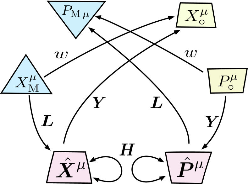
Figure 1: Schematic structure of the higher gauge symmetries: The different shapes of the objects indicate different scaling dimensions of canonical variables. The directions of arrows indicate how the variables are mixed into others (or into themselves) by gauge transformations. The row in the middle represents conserved vectors, while the top row represents the corresponding cyclic (passive) variables. Although superficially the transformations are acting symmetrically between the left and right sides of this diagram, their roles are different.

3 Bosonic action

We now have tools at our disposal to construct the action integral. For simplicity, we still concentrate to the bosonic part in this section. Our basic requirement is that the action should have symmetries, apart from the requirement of full SO(10,1) Lorentz-Poincaré invariance, under all transformations, namely, local $\tau$-reparametrizations, gauge transformations, as well as the global scale transformations and translations, which leave the canonical structure invariant. Up to total derivatives, unique possibility for the first-order (with respect to derivative) term is the Poincaré integral (62). As the simplest possible potential term satisfying these requirements, we choose using (15),

$$\frac{1}{12}\int d\tau\,e\,\langle[X^{\mu},X^{\nu},X^{\sigma}][X_{\mu},X_{\nu},X_{\sigma}]\rangle$$

$$= \frac{1}{4}\int d\tau\,e\,{\rm Tr}\Big{(}X_{{\rm{\tiny M}}}^{2}[\bm{X}^{\nu},\bm{X}^{\sigma}][\bm{X}_{\nu},\bm{X}_{\sigma}]-2[X_{{\rm{\tiny M}}}\cdot\bm{X},\bm{X}^{\nu}][X_{{\rm{\tiny M}}}\cdot\bm{X},\bm{X}_{\nu}]\Bigr{)}.$$ (64)

It is to be noted that the numerical proportional constant in front of the potential is arbitrary, since we can always absorb it by making a global rescaling $(X_{{\rm{\tiny M}}}^{\mu},P_{{\rm{\tiny M}}}^{\mu})\rightarrow(\rho X^{\mu}_{{\rm{\tiny M}}},\rho^{-1}P_{{\rm{\tiny M}}}^{\mu})$, $(B_{\circ},\bm{B})\rightarrow\rho^{-1}(B_{\circ},\bm{B})$ which keeps the the first-order term intact.

In order to have non-trivial dynamics, we need at least quadratic kinetic terms, typically as

$$-\int d\tau\,\frac{e}{2}{\rm Tr}(\bm{P}\cdot\bm{P}),$$

which however apparently violates gauge symmetry under (46). The symmetry can be recovered by the following procedure, which is analogous to a well known situation in the covariant field theory of a massive vector field. Namely, we introduce an auxiliary traceless matrix field $\bm{K}$ transforming simply as

$$\delta_{Y}\bm{K}=\bm{Y}.$$ (65)

Then, by replacing $\bm{P}^{\mu}$ as $\bm{P}^{\mu}\rightarrow\bm{P}^{\mu}-P_{\circ}^{\mu}\bm{K}$, we have an invariant quadratic kinetic term,

$$-\int d\tau\,\frac{e}{2}{\rm Tr}(\bm{P}-P_{\circ}\bm{K})^{2}=-\int d\tau\,\frac{e}{2}\Bigl{(}\frac{1}{N}P_{\circ}^{2}+{\rm Tr}(\hat{\bm{P}}-P_{\circ}\bm{K})^{2}\Bigr{)}.$$ (66)

The standard kinetic term without $\bm{K}$ is obtained by adopting $\bm{K}=0$ as the gauge condition. Since the equation of ‘motion’ (rather, another Gauss constraint) for $\bm{K}$ is

$$P_{\circ}\cdot(\hat{\bm{P}}-P_{\circ}\bm{K})=0,$$ (67)

this gauge choice is actually equivalent to the following choice of gauge condition

$$P_{\circ}\cdot\hat{\bm{P}}=0,$$ (68)

which renders the Gauss constraint (44) into a second-class constraint.

Putting together all the ingredients, the final form of bosonic action is

$$A_{{\rm boson}} =\int d\tau\Bigl{[}P_{\circ}\cdot\frac{DX_{\circ}}{D\tau}+P_{{\rm{\tiny M}}}\cdot\frac{dX_{{\rm{\tiny M}}}}{d\tau}+{\rm Tr}\Bigl{(}\hat{\bm{P}}\cdot\frac{D\hat{\bm{X}}}{D\tau}\Bigr{)}$$

$$-\frac{e}{2N}P_{\circ}^{2}-\frac{e}{2}\,{\rm Tr}(\hat{\bm{P}}-P_{\circ}\bm{K})^{2}+\frac{e}{12}\bigl{<}[X^{\mu},X^{\nu},X^{\sigma}][X_{\mu},X_{\nu},X_{\sigma}]\bigr{>}\Bigr{]}.$$ (69)

Clearly, this is the simplest possible non-trivial form of the action. The variation of the ein-bein $e$ gives the mass-shell constraint for the center-of-mass momentum

$$\qquad\qquad P_{\circ}^{2}+{\cal M}^{2}_{{\rm boson}}\simeq 0,$$ (70)

with the effective invariant mass-square ${\cal M}^{2}_{{\rm boson}}$ being given by

$${\cal M}^{2}_{{\rm boson}}=N{\rm Tr}(\hat{\bm{P}}-P_{\circ}\bm{K})^{2}-\frac{N}{6}\bigl{<}[X^{\mu},X^{\nu},X^{\sigma}][X_{\mu},X_{\nu},X_{\sigma}]\bigr{>},$$ (71)

which involves only the traceless matrices and is positive semi-definite on-shell with $\hat{\bm{P}}^{\mu}-P_{\circ}^{\mu}\bm{K}=\frac{1}{e}\frac{D\hat{\bm{X}}^{\mu}}{D\tau}$ under the Gauss constraints, since the time component of the traceless matrices are eliminated by these constraints: by the symbol $\simeq$ in (70), we indicate that the equality is valid in conjunction with the Gauss-law constraints,

$$[\bm{P}_{\mu},\bm{X}^{\mu}]=0,$$ (72)

$$\hat{\bm{P}}\cdot X_{{\rm{\tiny M}}}=0,$$ (73)

associated with the gauge fields $\bm{A}$ and $\bm{B}$, respectively, together with (43) and (44). It should be kept in mind that ultimately, after taking into account fermionic contribution to be discussed in the next section, we are interested in states for which the effective mass-square is of order one in the large $N$ limit.

In order to demonstrate that the above bosonic action has desirable properties as a covariantized version of Matrix theory, we now check some expected features.

(1) Consistency of the Gauss constraints with the equations of motion

As a first exercise, let us see briefly how the Gauss constraints (72) and (73) are consistent with the equations of motion,

$$\frac{d\hat{\bm{P}_{\mu}}}{d\tau}+ie[\bm{A},\bm{P}^{\mu}]=eP_{\circ\,\mu}\bm{Z}-\frac{e}{2N}\frac{\partial}{\partial\hat{\bm{X}}^{\mu}}{\cal M}^{2}_{{\rm boson}}.$$ (74)

The $\delta_{HL}$-gauge invariance of the potential is equivalent with the following identities.

$$X_{{\rm{\tiny M}}\,\mu}\frac{\partial}{\partial\bm{X}^{\mu}}{\cal M}^{2}_{{\rm boson}}=0,$$ (75)

$$[\bm{X}_{\mu},\frac{\partial}{\partial\bm{X}^{\mu}}{\cal M}^{2}_{{\rm boson}}]=0.$$ (76)

Then, by taking a contraction with $X_{{\rm{\tiny M}}}^{\mu}$ and using (43) with the conservation of $X_{{\rm M}}^{\mu}$, (74) leads to

$$\frac{d}{d\tau}(X_{{\rm M}}\cdot\hat{\bm{P}})+ie[\bm{A},X_{{\rm M}}\cdot\hat{\bm{P}}]=0.$$ (77)

On the other hand, by taking a commutator with $\bm{X}^{\mu}$ and using the first-order equations of motion for it

$$\hat{\bm{P}}^{\mu}-P_{\circ}^{\mu}\bm{K}=\frac{1}{e}\frac{d\hat{\bm{X}}^{\mu}}{d\tau}+i[\bm{A},\bm{X}^{\mu}]-X_{{\rm M}}^{\mu}\bm{B}$$ (78)

together with (44) and (67), we can derive

$$\frac{1}{e}\frac{d}{d\tau}\bigl{(}[\bm{X}^{\mu},\bm{P}_{\mu}]\bigr{)}=i[\bm{A},[\bm{X}^{\mu},\bm{P}_{\mu}]]+[\bm{B},X_{{\rm M}}\cdot\bm{P}],$$ (79)

ensuring the consistency of the Gauss constraints (72) and (73). The consistency of (43) and (44) with the equations of motion can also be easily checked: the conservation of $X_{{\rm M}}$ and $P_{\circ}^{\mu}$ ensures the time independence of (43), while contracting $P_{\circ\,\mu}$ with (78) gives

$$\frac{d}{d\tau}(P_{\circ}\cdot\hat{\bm{X}})+ie[\bm{A},P_{\circ}\cdot\bm{X}]-eP_{\circ}\cdot X_{{\rm M}}\hat{\bm{B}}=0.$$ (80)

One comment relevant here is that the dynamical role of the M-momentum $P_{{\rm{\tiny M}}}^{\mu}$ is to lead the conservation of $X_{{\rm{\tiny M}}}^{\mu}$, and that it does not participate in the dynamics of this system actively, since there is no kinetic term for it. Its behavior is determined by the equation of motion in terms of the other variables in a completely passive manner as

$$\frac{DP_{{\rm M}}^{\mu}}{D\tau}=-\frac{\partial}{\partial X_{{\rm{\tiny M}}\,\mu}}{\cal V},$$ (81)

where we denoted the potential term in the action by $-{\cal V}$. Note that the center-of-mass coordinate $X_{\circ}^{\mu}$ is also of passive nature, similarly, leading to the conservation of the center-of-mass momentum, and that its time derivative is expressed entirely in terms of the other variables. In other words, both these variables are “cyclic” variables using the terminology of analytical mechanics.

(2) Light-front and time-like gauge fixings

As a next check, let us demonstrate that this system reduces to the bosonic part of light-front Matrix theory after an appropriate gauge fixing together with the condition of compactification. Without losing generality, we first choose a two-dimensional (Minkowskian) plane spanned by two conserved vectors $P_{\circ}^{\mu}$ and $X_{{\rm{\tiny M}}}^{\mu}$ and introduce the light-front coordinates ($P^{\pm}_{\circ}\equiv P^{10}_{\circ}\pm P^{0}_{\circ}$ and $X_{{\rm{\tiny M}}}^{\pm}\equiv X^{10}_{{\rm{\tiny M}}}\pm X^{0}_{{\rm{\tiny M}}}$) foliating this plane. For convenience, we call this plane “M-plane”. Note that due to the space-like nature of $X_{{\rm{\tiny M}}}^{\mu}$ together with the constraint (43), both of its light-front components $X_{{\rm{\tiny M}}}^{\pm}$ are non-vanishing, while by definition two conserved vectors $P_{\circ}^{\mu}$ and $X_{{\rm{\tiny M}}}^{\mu}$ have no transverse components orthogonal to the M-plane. We can then choose the gauge using the $\delta_{L}$-gauge symmetry such that

$$\hat{\bm{X}}^{+}=0.$$ (82)

The remaining light-like component $\hat{\bm{X}}^{-}$ is in the second term of the potential term

$$\frac{1}{8}\int d\tau\,e\,{\rm Tr}([X_{{\rm{\tiny M}}}^{+}\bm{X}^{-},\bm{X}^{i}][X_{{\rm{\tiny M}}}^{+}\bm{X}^{-},\bm{X}^{i}]),$$ (83)

with $i$ running only over the SO(9) directions which are transverse to the M-plane. This is eliminated by the $\delta_{Y}$-Gauss constraint

$$0=P_{\circ}^{+}\hat{\bm{X}}^{-}+P_{\circ}^{-}\hat{\bm{X}}^{+}=P_{\circ}^{+}\hat{\bm{X}}^{-}\quad\Rightarrow\quad\hat{\bm{X}}^{-}=0,$$ (84)

under the condition $P_{\circ}^{+}\neq 0$. We stress that without this particular constraint we cannot derive the potential term coinciding with the light-front Matrix theory. As for the momentum variables, we can use the $\bm{B}$-gauge Gauss constraint

$$0=X_{{\rm{\tiny M}}}\cdot\hat{\bm{P}}=X^{-}_{{\rm{\tiny M}}}\hat{\bm{P}}^{+}+X_{{\rm{\tiny M}}}^{+}\hat{\bm{P}}^{-}\quad\Rightarrow\quad\bm{B}X_{{\rm{\tiny M}}}^{2}=0\quad\Rightarrow\quad\bm{B}=0,$$ (85)

with the assumption $X_{{\rm{\tiny M}}}^{2}>0$, using the first-order equations of motion after choosing the gauge condition $\bm{K}=0$ with respect to the $\delta_{w}$-gauge symmetry,

$$\hat{\bm{P}}^{\pm}=\frac{1}{e}\frac{d\hat{\bm{X}}^{\pm}}{d\tau}+i[\bm{A},\hat{\bm{X}}^{\pm}]-\bm{B}X_{{\rm{\tiny M}}}^{\pm}.$$ (86)

The result in the end is simply

$$\hat{\bm{P}}^{\pm}=0,$$ (87)

which also implies $\bm{Z}=0$ as a consequence of (74). Note also that the $\bm{A}$-gauge Gauss constraint takes the form

$$[\bm{X}_{i},\bm{P}_{i}]=0.$$ (88)

Now all light-like components of the traceless matrix variables are completely eliminated. The effective mass square in the light-front gauge takes the form

$${\cal M}^{2}_{{\rm bosonlf}}=N{\rm Tr}\Bigl{(}\hat{\bm{P}}_{i}\cdot\hat{\bm{P}}_{i}-\frac{1}{2}X_{{\rm{\tiny M}}}^{2}[\bm{X}_{i},\bm{X}_{j}][\bm{X}_{i},\bm{X}_{j}]\Bigr{)}.$$ (89)

From this result, it follows that the conserved Lorentz invariant $X_{{\rm{\tiny M}}}^{2}$ gives the 11 dimensional gravitational length as

$$X_{{\rm{\tiny M}}}^{2}=\frac{1}{\ell_{11}^{6}}.$$ (90)

The equations of motion for the center-of-mass variables and for $X_{{\rm{\tiny M}}}^{\mu}$ are, using $\hat{\bm{X}}^{\pm}=0$ and setting $ds=ed\tau$,

$$P_{\circ}^{\pm}=N\Bigl{(}\frac{dX_{\circ}^{\pm}}{ds}-B_{\circ}X_{{\rm{\tiny M}}}^{\pm}\Bigl{)},\quad\frac{dP^{\pm}_{\circ}}{ds}=0,\quad\frac{dX_{{\rm{\tiny M}}}^{\pm}}{ds}=0.$$ (91)

With respect to the $\delta_{w}$-gauge symmetry, we can choose a gauge $B_{\circ}=0$. Then,

$$P_{\circ}^{\pm}=N\frac{dX_{\circ}^{\pm}}{ds},$$ (92)

and we can identify the re-parametrization invariant time parameter $s$ with the center-of-mass light-front time coordinate as

$$X^{+}_{\circ}=\frac{P_{\circ}^{+}}{N}s.$$ (93)

The effective action for the remaining transverse variables is obtained by substituting the solutions of constraints resulting from the mass-shell condition

$$P_{\circ}^{-}=-\frac{{\cal M}^{2}_{{\rm lf}}}{P_{\circ}^{+}}$$ (94)

into the original action. Then, neglecting a total derivative, we obtain

$$A_{{\rm lf\,boson}} =\int ds\Bigl{[}{\rm Tr}\Bigl{(}\hat{\bm{P}}_{i}\frac{D\hat{\bm{X}_{i}}}{Ds}\Bigr{)}+\frac{1}{2}P_{\circ}^{-}\frac{dX^{+}_{\circ}}{ds}\Bigl{]}=\int ds\Bigl{[}{\rm Tr}\Bigl{(}\hat{\bm{P}}_{i}\frac{D\hat{\bm{X}_{i}}}{Ds}\Bigr{)}-\frac{1}{2N}{\cal M}_{{\rm bosonlf}}^{2}\Bigl{]}$$ (95)

$$\Rightarrow\int ds{\rm Tr}\Bigl{[}\frac{1}{2}\frac{D\hat{\bm{X}_{i}}}{Ds}\frac{D\hat{\bm{X}_{i}}}{Ds}+\frac{1}{4}X_{{\rm{\tiny M}}}^{2}[\bm{X}_{i},\bm{X}_{j}][\bm{X}_{i},\bm{X}_{j}]\Bigl{]}$$

$$=\int dx^{+}\frac{1}{2R}{\rm Tr}\Bigl{(}\frac{D\hat{\bm{X}}^{i}}{Dx^{+}}\frac{D\hat{\bm{X}_{i}}}{Dx^{+}}+\frac{R^{2}}{2\ell_{11}^{6}}[\bm{X}_{i},\bm{X}_{j}][\bm{X}_{i},\bm{X}_{j}]\Bigr{)},$$ (96)

where in the second line we shifted from our first-order form to the second-order formalism by integrating out the transverse momenta $\hat{\bm{P}}_{i}$, and in the third line, we have rescaled the time coordinate by $s=2Nx^{+}/P_{\circ}^{+}$ ($X_{\circ}^{+}=2x^{+}$) with the constant light-front momentum $P_{\circ}^{+}$ discretized with the DLCQ compactication by introducing a continuous parameter $R$ which can be changed arbitrarily by boost,

$$P_{\circ}^{+}=\frac{2N}{R}.$$ (97)

This condition expresses our premise that constituent partons all have the same basic unit $1/R$ of compactified momentum. Note also that it amounts to requiring that the relation between the light-front time $X_{\circ}^{+}$ and the invariant proper time $s$ is independent of $N$. Because of a global synchronization of the proper-time parameter as stressed in section 1, this is as it should be since the same relation between the target time and the proper time should hold for susbsystems when the system is regarded as a composite of many subsystems with smaller $N_{i}$’s such that $N=\sum_{i}N_{i}$. The gauge field $\bm{A}$ is also rescaled, $\bm{A}\rightarrow\frac{P_{\circ}^{+}}{2N}\bm{A}=\bm{A}/R$, and the covariant derivative is now without $\bm{B}$-gauge field since $X_{{\rm{\tiny M}}}^{i}=0$ as

$$\frac{D\hat{\bm{X}}^{i}}{Dx^{+}}=\frac{d\hat{\bm{X}}^{i}}{dx^{+}}+i[\bm{A},\bm{X}^{i}].$$ (98)

It is to be noted, as discussed in section 1, that if we set $R\Rightarrow R_{11}=g_{s}\ell_{s}$, this form (96) is identical with the low-energy effective action for D-particles in the weak-coupling limit $g_{s}\rightarrow 0$, giving an infinite momentum frame with fixed $N$ from a viewpoint of 11 dimensions as discussed in section 1.

Let us also briefly consider the case of a spatial compactification. We use the same frame for the two-dimensional M-plane spanned by $P_{\circ}^{\mu}$ and $X_{{\rm{\tiny M}}}^{\mu}$, but we foliate it in terms of the ordinary time coordinate $X_{\circ}^{0}$ and choose the time-like gauge

$$\hat{\bm{X}}^{0}=0,$$ (99)

which is possible since $X^{0}_{{\rm{\tiny M}}}\neq 0$ under the requirements $P_{\circ}^{10}>0,P_{\circ}^{0}>0$ due to the $\delta_{w}$-Gauss constraint (43). Then, the constraint (44) together with the $\bm{B}$-and-$\bm{Z}$-Gauss constraints leads to

$$\hat{\bm{X}}^{10}=0,$$ (100)

along with the corresponding momentum-space counterparts. Thus, as for the longitudinal component, we have the same results as the light-front case. Only difference is that the condition of compactification is, instead of (97),

$$P^{10}_{\circ}=\frac{N}{R_{11}},$$ (101)

and therefore the mass-shell constraint for the center-of-mass momentum is solved as

$$P_{\circ}^{0}=\sqrt{(P_{\circ}^{10})^{2}+N{\rm Tr}\Bigl{(}\hat{\bm{P}}_{i}\cdot\hat{\bm{P}}_{i}-\frac{1}{2}X_{{\rm{\tiny M}}}^{2}[\bm{X}_{i},\bm{X}_{j}][\bm{X}_{i},\bm{X}_{j}]\Bigr{)}},$$ (102)

which leads to the effective action

$$A_{{\rm spat\,boson}}=\int dt\Bigl{[}{\rm Tr}\Bigl{(}\hat{\bm{P}}_{i}\frac{D\hat{\bm{X}}_{i}}{Dt}\Bigr{)}-P_{\circ}^{0}\Bigr{]},$$ (103)

where we changed the parametrization by $t=X_{\circ}^{0}=\frac{P_{\circ}^{10}}{N}s=s/R_{11}$ and made a rescaling of the gauge field $\bm{A}$ correspondingly. On shifting to a first-order formalism by solving the momenta $\hat{\bm{P}}_{i}$ in terms of the coordinate variables, we arrive at a Born-Infeld-like action

$$A_{{\rm spat\,boson}}=-\int dt\,{\cal M}_{{\rm spat}}\sqrt{N}\Bigl{[}1-\frac{1}{N}{\rm Tr}\Bigl{(}\frac{D\hat{\bm{X}}_{i}}{Dt}\frac{D\hat{\bm{X}}_{i}}{Dt}\Bigr{)}\Bigr{]}^{1/2}$$ (104)

with

$${\cal M}_{{\rm spat}}\equiv\Bigl{[}\frac{N}{R_{11}^{2}}-\frac{1}{2\ell_{11}^{6}}{\rm Tr}\bigl{(}[\bm{X}_{i},\bm{X}_{j}][\bm{X}_{i},\bm{X}_{j}]\bigr{)}\Bigr{]}^{1/2},$$ (105)

which, in the limit of large $N$, can be approximated by

$$\int dt\,\frac{N}{R_{11}}\Bigl{[}-1+\frac{1}{2N}{\rm Tr}\Bigl{(}\frac{D\hat{\bm{X}}_{i}}{Dt}\frac{D\hat{\bm{X}}_{i}}{Dt}+\frac{R_{11}^{2}}{2\ell_{11}^{6}}[\bm{X}_{i},\bm{X}_{j}][\bm{X}_{i},\bm{X}_{j}]\Bigr{)}+O(\frac{1}{N^{2}})\Bigr{]},$$ (106)

as expected from the relation between the DLCQ scheme and the original BFSS proposal. Here it is assumed that both of the kinetic term ${\rm Tr}\Bigl{(}\frac{D\hat{\bm{X}}_{i}}{Dt}\frac{D\hat{\bm{X}}_{i}}{Dt}\Bigr{)}$ and the potential term ${\rm Tr}\bigl{(}[\bm{X}_{i},\bm{X}_{j}][\bm{X}_{i},\bm{X}_{j}]\bigr{)}$ are at most of order one.

After these non-covariant gauge fixings, the naive Lorentz transformation laws expressed by (63) must be modified by taking into account compensating gauge transformations. Though we do not work out formalistic details along this line, it is to be noted that such deformed transformation laws are necessarily different from those expected from the classical theory of membranes.

Remarks

(i) One of the novel characteristics in our model is that the 11 dimensional Planck length $\ell_{11}$ emerges as the expectation value (90) of an invariant $X_{{\rm{\tiny M}}}^{2}$, arising out of a completely scale-free theory. Together with a compactified unit $R_{11}$ (or $R$) of momentum, they provide two independent constants $g_{s}$ and $\ell_{s}$ of string theory embedded in 11 dimensions. This emerges once we specify a particular solution for $P_{\circ}^{\mu}$ and $X_{{\rm M}}^{\mu}$ as initial conditions through these conserved quantities. However, the meaning of the Lorentz invariant $X_{{\rm{\tiny M}}}^{2}$ is quite different from $P_{\circ}^{\mu}$. The former determines the coupling constant for the time-evolution of traceless matrix variables in a Lorentz-invariant manner, while the latter only specifies the initial values of center-of-mass momentum which is essentially decoupled from the dynamics of the traceless matrix part. It seems natural to postulate that the invariant $X_{{\rm{\tiny M}}}^{2}$ defines a super-selection rule with respect to the scale symmetry of our system. In other words, we demand that no superposition is allowed among states with different values of $X_{{\rm{\tiny M}}}^{2}$. Due to the scale symmetry, any pair of different sectors of the Hilbert space (after quantization) can be mapped into each other by an appropriate scale transformation, and then all the different super-selection sectors describe completely the same dynamics. In this sense, the scale symmetry is spontaneously broken. Such a fundamental nature of 11 dimensional gravitational length is also one of the expected general properties of M-theory.

On the other hand, states with varying components of the vector $X_{{\rm{\tiny M}}}^{\mu}$ connected by Lorentz transformations with a fixed $X_{{\rm M}}^{2}$ are not forbidden to be superposed, along with the center-of-mass momentum $P_{\circ}^{\mu}$. In fact, the $\delta_{w}$-gauge Gauss constraint (43) requires this: depending on the light-front foliation or time-like foliation, it leads to relations among these conserved quantities, respectively,

$$P_{\circ}^{-}=-\frac{P_{\circ}^{+}}{(X_{{\rm{\tiny M}}}^{+})^{2}}X_{{\rm{\tiny M}}}^{2}\qquad\mbox{or}\qquad P_{\circ}^{0}=\frac{P_{\circ}^{10}X_{{\rm{\tiny M}}}^{10}}{\sqrt{(X_{{\rm{\tiny M}}}^{10})^{2}-X_{{\rm{\tiny M}}}^{2}}}.$$ (107)

Thus, given the center-of-mass “energies”, compactification radii and gravitational length, these relations determine $X_{{\rm{\tiny M}}}^{+}$ or $X_{{\rm{\tiny M}}}^{10}$. In particular, the light-like limit $P_{\circ}^{-}\rightarrow 0$ with finite $P_{\circ}^{+}$ (or $P_{\circ}^{10}$) corresponds to a singular limit $X_{{\rm{\tiny M}}}^{+}\rightarrow\infty$ or equivalently to $X_{{\rm{\tiny M}}}^{10}\rightarrow\infty$.

(ii) The fact that the system is reducible from 11 (10 spatial and 1 time-like) matrix degrees of freedom to 9 spatial matrix degrees of freedom is of course due to the presence of the higher gauge symmetries. From the viewpoint of ordinary relativistic mechanics of many particles, this feature is also quite a peculiar phenomenon: our higher gauge symmetries imply that two space-time directions corresponding to the M-plane are locally unobservable with respect to the dynamics of M-theory partons. That is the reason why we can eliminate both of the traceless parts, $\hat{\bm{X}}^{\pm}$ and $\hat{\bm{P}}^{\pm}$ of the matrix degrees of freedom along the M-plane. If $X_{{\rm M}}^{+}\hat{\bm{X}}^{-}$ in (83) were not eliminated in the above light-front gauge fixing, we would have $-\bigl{(}X_{{\rm M}}^{+}X^{-}_{ab}(x_{a}^{i}-x_{b}^{i})\bigr{)}^{2}$ giving non-zero potential of wrong sign for purely diagonal configurations with respect to the transverse directions. The absence of this term conforms to, at least qualitatively, one remarkable aspect of general-relativistic interactions of M-theory partons. Due to the elimination of $\hat{\bm{X}}^{-}$, the static diagonal matrices (with $\hat{\bm{P}}^{i}=0$ and $[\bm{X}_{i},\bm{X}_{j}]=0$) for all directions transverse to the plane spanned by $P_{\circ}^{\mu}$ and $X_{{\rm{\tiny M}}}^{\mu}$ provide exact classical solutions describing degenerate ground states with ${\cal M}_{{\rm boson}}^{2}=0$, corresponding to the flat directions of the potential term, whose existence is also a consequence of the structure of our 3-bracket. In classical particle pictures, this corresponds to bundles of parallel (and collinear as a special degenerate limit) trajectories of 11 dimensional gravitons. On the other hand, in classical general relativity, it is well known that the parallel pencil-like trajectories of massless particles are non-interacting: equivalently, for the metric of the form

$$ds^{2}=dx^{\mu}dx_{\mu}+h_{--}(dx^{-})^{2}$$ (108)

with coordinate condition $\partial_{+}h_{--}=0$, the vacuum Einstein equations reduce to the linear Laplace equation $\partial_{i}^{2}h_{--}=0$ in the transverse space around such trajectories [18]. This makes possible the interpretation of states with higher quantized momenta $P^{+}_{\circ}$ as composite states consisting of constituent states with unit momentum $1/R$ along the compactified direction. Note that in ordinary local theories of point-like particles, a state of a single particle with multiple units of momentum and a state of many particles of the same total momentum but with various different distributions of constitutent’s momenta must be treated as different states which can be discriminated by relative positions in the coordinate representation. In contrast to this, our higher gauge symmetries render the relative positions along the $x^{-}$ directions unobservable as unphysical degrees of freedom.

(iii) As regards classical solutions with diagonal transverse degrees of matrices, there is another curious property for non-static solutions with constant non-zero velocities for finite $N$. The action (104) in the time-like gauge shows that the upper bound for the magnitude of transverse relative velocities is described by

$$N\geq{\rm Tr}\Bigl{(}\frac{D\hat{\bm{X}}_{i}}{Dt}\frac{D\hat{\bm{X}}_{i}}{Dt}\Bigr{)}$$ (109)

For classical diagonal configurations with vanishing gauge fields, the right-hand side reduces to the sum of squared velocities $\sum_{a=1}^{N}\bigl{(}d\hat{X}_{aa}^{i}/dt)^{2}$, and hence for symmetric distributions of D-particles such that $v\equiv|d\hat{X}_{aa}^{i}/dt|$ is indenpendent of $a$, this bound corresponds to the usual relativistic bound $v\leq c=1$ in terms of absolute (not relative) velocities. On the other hand, for non-symmetrical configurations, this, being a bound averaged over relative velocities of constituent partons and the off-diagonal degrees of freedom, does not forbid the appearance of super-luminal velocities for a part of constituent partons, when other partons have sub-luminal (or zero) velocities provided $N\geq 3$. This situation is owing to the absence of the mass-shell conditions set independently for each parton, and is actually expected in any covariantized extensions of the light-front super quantum mechanics, which itself has no such condition, as we have already mentioned in the Introduction. Note, however, that the role of these peculiar states would be negligible in any well defined large $N$ limits of our interest.

4 Fermionic degrees of freedom and supersymmetry

Our next task is to extend foregoing constructions to a supersymmetric theory. Since we already know a supersymmetric version reduced to the light-front gauge with the DLCQ compactification, all we need is to find a way of reformulating it in terms of appropriate languages which fit consisitently to the structure of the previous bosonic part without violating covariance in the sense of 11 dimensional Minkowski space-time and other symmetries. Corresponding to the traceless part of the bosonic matrices, we introduce Majonara spinor Hermitian traceless matrices denoted by $\bm{\Theta}$. By this, we mean that all the would-be real components of matrix elements are Majonara spinors with 32 components. The Dirac conjugate is defined by $\bar{\bm{\Theta}}_{ab}=\bm{\Theta}^{{\rm T}}_{ab}\Gamma^{0}$ where the transposition symbol T is with resect to spinor components treated as column and row vectors; but we mostly suppress the T-symbol on $\bm{\Theta}$ below, because it must be obvious by the position of Gamma matrices acting on them.

To be a supersymmetric theory, we also need the fermionic partner for the center-of-mass degrees of bosonic variables. The fermionic center-of-mass degrees of freedom, being a single 32 component Majorana spinor, are denoted by $\Theta_{\circ}$ with the subscript $\circ$ as in the bosonic case. Unlike bosonic case, the relative normalization between the traceless fermion matrices and $\Theta_{\circ}$ can be chosen arbitrarily since it is completely decoupled from the dynamics of the traceless matrices. We therefore treat the fermionic matrices $\bm{\Theta}$ always as traceless, being completely separated from the center-of-mass fermionic variables $\Theta_{\circ}$. Note that in the bosonic case, the center-of-mass motion couples with the traceless part through the Hamiltonian constraint, although their equations of motion are decoupled. Under the $\tau$-reparametrization, both $\Theta_{\circ}$ and $\bm{\Theta}$ transform as scalar.

We aim at a minimally possible extension of the light-front Matrix theory. A fundamental premise in what follows is that for fermionic variables, there is no counterpart of the bosonic M-variables, a canonical (non-matrix) pair $(X_{{\rm{\tiny M}}}^{\mu},P_{{\rm{\tiny M}}}^{\mu})$. This requires that the Gauss constraints (43) and (73) involving them must themselves be invariant under supersymmetry transformations. This will be achieved by requiring that the center-of-mass momentum $P_{\circ}^{\mu}$ is super invariant, and consequently the Gauss constraint (44) should also be super invariant. To be consistent with these demands, the fermionic variables are not subject to gauge transformations except for $\delta_{HL}\Theta=\delta_{HY}\Theta=\delta_{H}\Theta=(0,i\sum_{r}[F^{r},G^{r},\Theta])$, which is reduced simply only to the usual SU($N$) gauge transformation corresponding to the gauge field $\bm{A}$,

$$\delta_{H}\bm{\Theta}=i[\bm{H},\bm{\Theta}].$$ (110)

Consequently the usual traces of the products of fermion matrices give gauge invariants, provided they do not involve bosonic matrix variables, while the products involving both fermionic and bosonic matrices can be made invariant by combining them into 3-brackets, just as in the case of purely bosonic cases. Since the fermionic variables intrinsically obey the first-order formalism in which the generalized coordinates and momenta are mixed inextricably among spinor components and hence the fermionic generalized coordinates and momenta should have the same transformation laws, it would be very difficult to extend the structure of higher-gauge transformations for the bosonic variables to fermionic variables covariantly if we assumed non-zero fermionic M-variables. But that is not necessary as we shall argue below.

4.1 Center-of-mass part: 11 dimensional rigid supersymmetry

Let us now start from the center-of-mass degrees of freedom. Since we require that the theory has at least 11 dimensional rigid supersymmetry, it is natural to set the center-of-mass part in a standard fashion as for the case of a single point particle. Thus the fermionic action is chosen to be

$$\int d\tau P_{\circ\,\mu}\bar{\Theta}_{\circ}\Gamma^{\mu}\frac{d\Theta_{\circ}}{d\tau},$$ (111)

which is obtained by making a replacement $\frac{dX^{\mu}_{\circ}}{d\tau}\rightarrow\frac{dX^{\mu}_{\circ}}{d\tau}+\bar{\Theta}_{\circ}\Gamma^{\mu}\frac{d\Theta_{\circ}}{d\tau}$ from the center-of-mass part of the bosonic Poincaré integral. Under the usual rigid super translation

$$\delta_{\varepsilon}\Theta_{\circ}=-\varepsilon,$$ (112)

together with the requirement

$$\delta_{\varepsilon}P_{\circ}^{\mu}=0,$$ (113)

the action is invariant by assuming the transformation law for the bosonic center-of-mass coordinates as

$$\delta_{\varepsilon}X_{\circ}^{\mu}=\bar{\varepsilon}\Gamma^{\mu}\Theta_{\circ},$$ (114)

since

$$\delta_{\varepsilon}\Bigl{(}\frac{dX^{\mu}_{\circ}}{d\tau}+\bar{\Theta}_{\circ}\Gamma^{\mu}\frac{d\Theta_{\circ}}{d\tau}\Bigr{)}=0,$$ (115)

which is consistent with the first order equations of motion.

Under the assumption that all the other variables not exhibited above are inert with respect to the rigid super transformation, it is clear that the existence of these fermionic center-of-mass degrees of freedom does not spoil any of symmetry properties introduced in previous sections, provided that the remaining matrix part of the action decouples from $X_{\circ}^{\mu},\Theta_{\circ}$ and $P_{{\rm M}}^{\mu}$. This ensures that the first-order equations of motion for the canonical pairs $(X_{\circ}^{\mu},P_{\circ}^{\mu})$ and $(X_{{\rm M}}^{\mu},P_{{\rm M}}^{\mu})$ are of the following form, reflecting conservation laws and the passive nature of the associated cyclic variables,

$$\frac{dP_{\circ}^{\mu}}{d\tau}=0,$$ (116)

$$\frac{1}{e}\Bigl{(}\frac{DX_{\circ}^{\mu}}{D\tau}+\bar{\Theta}_{\circ}\Gamma^{\mu}\frac{d\Theta_{\circ}}{d\tau}\Bigr{)}=P_{\circ}^{\mu}-f^{\mu},$$ (117)

$$\frac{dX_{{\rm M}}^{\mu}}{d\tau}=0,$$ (118)

$$\frac{1}{e}\frac{DP_{{\rm M}}^{\mu}}{D\tau}=g^{\mu},$$ (119)

where the unspecified functions $f^{\mu}$ and $g^{\mu}$ are contributions from the remaining part of action and do not depend on these passive variables themselves. It should also be mentioned that the scale dimensions of the fermion center-of-mass variables are

$$\Theta_{\circ}\rightarrow\lambda^{1/2}\Theta_{\circ},\quad\varepsilon\rightarrow\lambda^{1/2}\varepsilon.$$ (120)

The equation of motion for the fermionic center-of-mass spinor is then

$$P_{\circ}\cdot\Gamma\frac{d\Theta_{\circ}}{d\tau}=0.$$ (121)

For generic case with non-vanishing effective mass square $-P_{\circ}^{2}>0$, this leads to a conservation law

$$\frac{d\Theta_{\circ}}{d\tau}=0.$$ (122)

In general, the quantum states consist of fundamental massive super-multiplets of dimension $2^{16}$.

We here briefly touch the canonical structure of the fermionic center-of-mass variables. From the above action, there is a primary second-class constraint,

$$\Pi_{\circ}+\bar{\Theta}P_{\circ}\cdot\Gamma=0,$$ (123)

satisfying a Poisson bracket relation

$$\{\Pi_{\circ\,\alpha}+(\bar{\Theta}P_{\circ}\cdot\Gamma)_{\alpha},\Pi_{\circ\,\beta}+(\bar{\Theta}P_{\circ}\cdot\Gamma)_{\beta}\}_{{\rm P}}=2(\Gamma^{0}P_{\circ}\cdot\Gamma)_{\alpha\beta},$$ (124)

where $\Pi_{\circ}$ is canonically conjugate to $\Theta_{\circ}$ and $\alpha,\beta,\ldots$ are spinor indices. Correspondingly, the Poisson bracket must be replaced by Dirac bracket, which is also required to render the canonical structure supersymmetric. We give a brief account of this topic in appendix A.

In the limit of light-like center-of-mass momentum $P_{\circ}^{2}=0$, a one-half of the primary constraints (123) becomes first class because of the existence of zero eigenvalues for the Dirac operator $P_{\circ}\cdot\Gamma$, and the fermionic equations of motion have a redundancy. In the present work, we will not elaborate on remedying this complication, by assuming generic massive case. Physically, this is allowed since the system, describing a general many-body system with massless gravitons, has continuous mass spectrum without mass gap. When we have to deal with the light-like case, we can always consider a slightly different state with a small but non-zero center-of-mass by adding soft gravitons propagating with a non-zero small momentum along directions transverse to the original states.

As is well known, the singularity at $P_{\circ}^{2}=0$ is associated with the emergence of a local symmetry, called Siegel (or “$\kappa$”-) symmetry [19],

$$\delta_{\kappa}\Theta_{\circ}=P_{\circ}\cdot\Gamma\kappa,\quad\delta_{\kappa}X_{\circ}^{\mu}=-\bar{\Theta}_{\circ}\Gamma^{\mu}\delta_{\kappa}\Theta_{\circ},$$ (125)

with arbitrary spinor function $\kappa(\tau)$. This allows us to eliminate a half of components of $\Theta_{\circ}$ by a suitable redefinition of $X_{\circ}^{\mu}$, and hence the super-multiplets are shorten to $2^{16/2}=2^{8}=256$ dimensions (or to half-BPS states). This coincides with the dimension of graviton super-multiplet in 11 dimensions which constitutes the basic physical field-degrees of freedom of 11 dimensional supergravity. It should be noted, however, that generic many-body states with time-like center-of-mass momenta composed of massless short multiplets obey “longer” massive representations. For instance, a generic two-body scattering state of gravitons with $-P_{\circ}^{2}>0$ would constitute a massive multiplet of $2^{8}\times 2^{8}=2^{16}$ dimensions. Therefore, it does not seem reasonable to demand a $\kappa$-symmetry as a general condition in our case of the center-of-mass supersymmetry, since we are dealing with $N=1$ supersymmetry in the highest 11 dimensions.

4.2 Traceless matrix part: dynamical supersymmetry

Next, we proceed to the traceless matrix part. A natural candidate for the transformation law of the bosonic matrices is

$$\delta_{\epsilon}\hat{\bm{X}}^{\mu}=\bar{\epsilon}\Gamma^{\mu}\bm{\Theta}.$$ (126)

Superficially the previous transformation (114) may be regarded as the trace part of this form, but we will shortly see critical differences. To keep the difference in mind, the spinor parameter is now denoted by a symbol $\epsilon$ which is distinct from that ($\varepsilon$) for the center-of-mass degrees of freedom, since they are in principle independent of each other and can be treated separately. This is natural, since the traceless matrices describe the internal dynamics of relative degrees of freedom. Following common usage, we call the rigid supersymmetry of the center-of-mass part “kinematical” which is essentially a superspace translation as a partner of rigid space-time translation, and that of the traceless part “dynamical”, mixing between the bosonic and fermionic traceless matrices without any inhomogeneous shift-type contributions. The dynamical supersymmetry of our system will be related to rigid translations with respect to the invariant time parameter $s$ ($ds=ed\tau$). Once these two independent supersymmetries are established, however, we can combine them depending on different situations. For instance, we can partially identify $\epsilon$ and $\varepsilon$ up to some proportional factor and projection (or twisting) conditions with respect to spinor indices. That would occur through an identification of the invariant proper-time parameter with an external time coordinate as a gauge choice for re-parametrization invariance, as in the case of the usual formulation of the light-front Matrix theory.

(1) Projection conditions

In discussing the transformation law for $\bm{\Theta}$, we have to take into account the existence of the Gauss constraint (43) which characterizes the M-plane. We treat this constraint as a strong constraint in studying dynamical supersymmetry. This is allowed, as long as Lorentz covariance is not lost. We then have to assume the equations of motion for the center-of-mass part and for the M-variables strongly, so that we can use the conservation laws of $P_{\circ}^{\mu}$ and $X_{{\rm{\tiny M}}}^{\mu}$, both of which are assumed to be inert $\delta_{\epsilon}P^{\mu}_{\circ}=0=\delta_{\epsilon}X^{\mu}_{{\rm M}}$ against dynamical as well as kinematical super transformations. We do not expect any difficulty with this restriction at least practically: for example, we can use the representation where both of these vectors are diagonalized for quantization. Thus it should be kept in mind that the supersymmetry transformation laws derived below have validity only “on shell” with respect to these variables. With respect to the traceless matrix part, on the other hand, they will be valid without using the equations of motion.

Now we have to examine the compatibility of the other Gauss constraints (44) and (73) with dynamical supersymmetry. Our assumptions, with the dynamical super transformation (126), requires that $\delta_{\epsilon}(P_{\circ}\cdot\hat{\bm{X}})=0$, namely,

$$\bar{\epsilon}P_{\circ}\cdot\Gamma\bm{\Theta}=0.$$ (127)

It is also necessary to demand $\delta_{\epsilon}(X_{{\rm M}}\cdot\hat{\bm{P}})=0$ for the momentum as

$$X_{{\rm M}}\cdot\delta_{\epsilon}\hat{\bm{P}}=0.$$ (128)

We first concentrate on the former. In any natural decomposition between generalized coordinates and momenta for the spinor components of $\bm{\Theta}$, this is a second-class constraint. This suggests that the traceless spinor matrix and parameter $\epsilon$ should obey certain projection condition strongly, rather than as a Gauss constraint associated with gauge symmetry, such that (127) is obeyed. By the existence of two conserved vectors $P_{\circ}^{\mu}$ and $X_{{\rm{\tiny M}}}^{\mu}$ which are orthogonal to each other due to the strong constraint (43), we have a candidate for Lorentz-invariant (real) projector:

$$P_{\pm}\equiv\frac{1}{2}(1\pm\Gamma_{\circ}\Gamma_{{\rm{\tiny M}}}).$$ (129)

Here we have introduced

$$\Gamma_{{\rm{\tiny M}}}\equiv\frac{X_{{\rm{\tiny M}}}\cdot\Gamma}{\sqrt{X_{{\rm{\tiny M}}}^{2}}},\quad\Gamma_{\circ}\equiv\frac{P_{\circ}\cdot\Gamma}{\sqrt{-P_{\circ}^{2}}},$$ (130)

by assuming generic cases with time-like center-of-mass momentum $-P_{\circ}^{2}>0$ as before. Due to the orthogonality constraint (43), these Lorentz-invariant Dirac matrices satisfy

$$\Gamma_{{\rm{\tiny M}}}\Gamma_{\circ}+\Gamma_{\circ}\Gamma_{{\rm{\tiny M}}}=0,\quad\Gamma_{{\rm{\tiny M}}}^{2}=1,\quad\Gamma_{\circ}^{2}=-1,\quad(\Gamma_{\circ}\Gamma_{{\rm{\tiny M}}})^{2}=1,$$ (131)

and consequently

$$\Gamma_{{\rm{\tiny M}}}(\Gamma_{\circ}\Gamma_{{\rm{\tiny M}}}) =-(\Gamma_{\circ}\Gamma_{{\rm{\tiny M}}})\Gamma_{{\rm{\tiny M}}},\quad\Gamma_{\circ}(\Gamma_{\circ}\Gamma_{{\rm{\tiny M}}})=-(\Gamma_{\circ}\Gamma_{{\rm{\tiny M}}})\Gamma_{\circ},$$ (132)

$$P_{+}\Gamma_{{\rm{\tiny M}}}=\Gamma_{{\rm{\tiny M}}}P_{-},\,\,P_{+}\Gamma_{\circ}=\Gamma_{\circ}P_{-},$$ (133)

$$P_{\pm}^{2}=P_{\pm},\,P_{\pm}P_{\mp}=0.$$ (134)

Note that

$$P_{\pm}\Gamma_{i}=\Gamma_{i}P_{\pm}$$ (135)

for the SO(9) directions $i$, transverse to the M-plane.

We then introduce the projection condition by $\Gamma_{\circ}\Gamma_{{\rm{\tiny M}}}\bm{\Theta}=-\bm{\Theta}$, namely,

$$P_{-}\bm{\Theta}=\bm{\Theta},\,\,P_{+}\bm{\Theta}=0,\quad\mbox{(or \,\, equivalently \,\, $\bar{\bm{\Theta}}P_{+}=\bar{\Theta},\,\,\bar{\bm{\Theta}}P_{-}=0$)}$$ (136)

together with the opposite projection on $\epsilon$,

$$P_{+}\epsilon=\epsilon,\,\,P_{-}\epsilon=0,\quad\mbox{(or \,\, equivalently \,\, $\bar{\epsilon}P_{-}=\bar{\epsilon},\,\,\bar{\epsilon}P_{+}=0$)}.$$ (137)

Then as desired

$$\bar{\epsilon}P_{\circ}\cdot\Gamma\bm{\Theta}=\bar{\epsilon}P_{-}(P_{\circ}\cdot\Gamma)P_{-}\bm{\Theta}=\bar{\epsilon}(P_{\circ}\cdot\Gamma)P_{+}P_{-}\bm{\Theta}=0,$$ (138)

and simultaneously we also have,

$$\bar{\epsilon}X_{{\rm{\tiny M}}}\cdot\Gamma\bm{\Theta}=\bar{\epsilon}P_{-}(X_{{\rm{\tiny M}}}\cdot\Gamma)P_{-}\bm{\Theta}=\bar{\epsilon}X_{{\rm{\tiny M}}}\cdot\Gamma P_{+}P_{-}\bm{\Theta}=0,$$ (139)

while

$$\bar{\epsilon}\Gamma_{i}\bm{\Theta}=\bar{\epsilon}P_{-}\Gamma_{i}P_{-}\bm{\Theta}=\bar{\epsilon}\Gamma_{i}P_{-}\bm{\Theta}=\bar{\epsilon}P_{-}\Gamma_{i}\bm{\Theta}$$ (140)

can be non-vanishing for all $i$’s, transverse to both $P_{\circ}$ and $X_{{\rm{\tiny M}}}$. The dynamical supersymmetry is thus effective essentially in the directions which are transverse to the M-plane, in conformity with our requirement. This automatically ensures the remaining requirement (128), as we will confirm later.

It is to be noted that the condition (136) is equivalent to

$$(\Gamma_{\circ}-\Gamma_{{\rm{\tiny M}}})\bm{\Theta}=0,$$ (141)

which can be regarded as a Lorentz-covariant version of a familiar light-front gauge condition $\Gamma^{+}\bm{\Theta}=0$. In fact, using the light-front frame defined in the previous section, we can rewrite (141) using (107) as ($\Gamma^{\pm}=\Gamma^{10}\pm\Gamma^{0}$)

$$0 =\frac{1}{2\sqrt{-P_{\circ}^{2}}}\Bigl{(}P_{\circ}^{+}\Gamma^{-}+P_{\circ}^{-}\Gamma^{+}-\frac{\sqrt{-P_{\circ}^{+}P_{\circ}^{-}}}{\sqrt{X_{{\rm{\tiny M}}}^{2}}}(X_{{\rm{\tiny M}}}^{+}\Gamma^{-}+X_{{\rm{\tiny M}}}^{-}\Gamma^{+})\Bigr{)}\bm{\Theta}$$

$$=\frac{1}{2\sqrt{-P_{\circ}^{2}}}\Bigl{(}P_{\circ}^{+}\Gamma^{-}+P_{\circ}^{-}\Gamma^{+}-\frac{P_{\circ}^{+}}{X_{{\rm{\tiny M}}}^{+}}(X_{{\rm{\tiny M}}}^{+}\Gamma^{-}+\frac{X_{{\rm{\tiny M}}}^{2}}{X_{{\rm{\tiny M}}}^{+}}\Gamma^{+})\Bigr{)}\bm{\Theta}=-\sqrt{-\frac{P_{\circ}^{-}}{P_{\circ}^{+}}}\Gamma^{+}\bm{\Theta}.$$ (142)

In the classical theory of a single supermembrane, the possibility of a similar projection owes to the existence of the $\kappa$-symmetry. In our system, by contrast, the existence of the gauge-invariant Gauss constraints in the bosonic sector, involving dynamical variables without fermionic partners, requires us, on our premise of a minimal extension, necessarily to introduce projection condition for fermionic variables in a Lorentz-covariant and gauge-invariant manner. Thus our strategy can be different: we need not bother about possible imposition of a generalized $\kappa$-like symmetry for traceless matrix variables. The dynamical supersymmetry requires that the physical degrees of freedom of traceless matrices match between bosonic and fermionic variables. On the bosonic side, the number of physical degrees of freedom after imposing all contraints is 8, counting the pairs of canonical variables, if we take into account all of the Gauss constraints including the $\bm{A}$-gauge symmetry. The number of physical degrees of freedom for the fermionic traceless matrices must therefore be 16, and this was made possible by our covariant projection condition (136) as a partner of the bosonic constraints represented by the set of Gauss constraints, thanks to the existence of the M-variables.

(2) Fermion action and dynamical supersymmetry transformations

We are now ready to present the fermionic part of the action and supersymmetry transformations. The total fermionic contribution to be added to the bosonic action (69) is

$$A_{{\rm fermion}}=\int d\tau\,\Bigl{[}\bar{\Theta}_{\circ}P_{\circ}\cdot\Gamma\frac{d\Theta_{\circ}}{d\tau}+\frac{1}{2}{\rm Tr}\Bigl{(}\bar{\bm{\Theta}}\Gamma_{\circ}\frac{D\bm{\Theta}}{D\tau}\Bigr{)}-e\frac{i}{4}\bigl{<}\bar{\Theta},\Gamma_{\mu\nu}[X^{\mu},X^{\nu},\Theta]\bigr{>}\Bigr{]}.$$ (143)

In the matrix form, the 3-bracket in the fermionic potential term is equal to

$$\bigl{<}\bar{\Theta},\Gamma_{\mu\nu}[X^{\mu},X^{\nu},\Theta]\bigr{>} =2\sqrt{X_{{\rm M}}^{2}}{\rm Tr}\bigl{(}\bar{\bm{\Theta}}\Gamma_{\circ}\Gamma_{i}[\bm{X}_{i},\bm{\Theta}]\bigr{)}=2\sqrt{X_{{\rm M}}^{2}}{\rm Tr}\bigl{(}\bar{\bm{\Theta}}\Gamma_{\circ}\Gamma_{\mu}[\bm{X}^{\mu},\bm{\Theta}]\bigr{)},$$ (144)

due to the projection condition and the fact that no M-variables are associated with fermionic matrices. A consequence of this is that, due to the fermion projection condition, (144) depends on the coordinate matrices only of directions transverse to the M-plane.

It is to be noted here that the traceless fermion matrices have zero scaling dimensions, with the dimension of $\epsilon$ being 1 correspondingly, in contrast to the case of center-of-mass fermion variables $\Theta_{\circ}$ and $\varepsilon$ whose scale dimensions are both 1/2. This convention is convenient here to simplify some of the expressions, and no inconsistency arises as noticed before, since there is no coupling between $\Theta_{\circ}$ and $\bm{\Theta}$, and the kinematical supersymmetry transformation of the latter can be discussed independently of the former dynamical supersymmetry.

The dynamical supersymmetry transformations for matrix variables are, with the projection conditions (136), (137) and the Gauss constraint (43) for the $\delta_{w}$-gauge symmetry,

$$\delta_{\epsilon}\hat{\bm{X}}^{\mu}=\bar{\epsilon}\Gamma^{\mu}\bm{\Theta},$$ (145)

$$\delta_{\epsilon}\hat{\bm{P}}_{\mu}=i\sqrt{X_{{\rm{\tiny M}}}^{2}}\,\bigl{[}\bar{\bm{\Theta}}\Gamma_{\mu\nu}\epsilon,\tilde{\bm{X}}^{\nu}],\quad\delta_{\epsilon}\bm{K}=0,$$ (146)

$$\delta_{\epsilon}\bm{\Theta}=P_{-}\bigl{(}\Gamma_{\circ}\Gamma_{\mu}\hat{\bm{P}}^{\mu}\epsilon-\frac{i}{2}\sqrt{X_{{\rm{\tiny M}}}^{2}}\,\Gamma_{\circ}\Gamma_{\mu\nu}\epsilon[\tilde{\bm{X}}^{\mu},\tilde{\bm{X}}^{\nu}]\bigr{)},$$ (147)

$$\delta_{\epsilon}\bm{A}=\sqrt{X_{{\rm{\tiny M}}}^{2}}\,\bar{\bm{\Theta}}\epsilon,$$ (148)

$$\delta_{\epsilon}\bm{B}=i\bigl{(}X_{{\rm{\tiny M}}}^{2}\bigr{)}^{-1}[\delta_{\epsilon}\bm{A},X_{{\rm{\tiny M}}}\cdot\bm{X}],$$ (149)

$$\delta_{\epsilon}\bm{Z}=i(P_{\circ}^{2})^{-1}[\delta_{\epsilon}\bm{A},P_{\circ}\cdot\bm{P}]+\frac{X_{{\rm M}}^{2}}{2P_{\circ}^{2}}([\delta_{\epsilon}\bm{X}^{\mu},[P_{\circ}\cdot\bm{X},\bm{X}_{\mu}]]+[\bm{X}^{\mu},[P_{\circ}\cdot\bm{X},\delta_{\epsilon}\bm{X}_{\mu}]])$$ (150)

with

$$\tilde{\bm{X}}^{\mu}=\bm{X}^{\mu}-\frac{1}{X_{{\rm{\tiny M}}}^{2}}X_{{\rm{\tiny M}}}^{\mu}(\bm{X}\cdot X_{{\rm{\tiny M}}})-\frac{1}{P_{\circ}^{2}}P_{\circ}^{\mu}(\bm{X}\cdot P_{\circ}).$$ (151)

It is easy to check that due to our projection condition, (128) is satisfied as promised before. Remember again that, as we have emphasized, the equations of motion for the center-of-mass variables and the M-variables, especially conservation laws of $P_{\circ}^{\mu}$ and $X_{{\rm M}}^{\mu}$ which are completely inert against supersymmetry transformations as well as gauge transformaionts, are assumed here. On the other hand, the behavior of their conjugates, namely the passive variables, are fixed by the first order equations of motion. It is also to be noted that these transformation laws are independent of the ein-bein $e$. This implies that the part of the action involving $\tau$-derivatives and the remaining part (essentially Hamiltonian ${\cal H}$) including contributions with gauge fields, which does not involve the $\tau$-derivatives being proportional to the ein-bein $e$ are separately invariant under the supersymmetry transformations. This is one of the merits of the first-order formalism. A derivation of these results will be found in appendix B.

In order to express the properties of these transformation laws from the viewpoint of canonical formalism, we need Dirac bracket. Here for simplicity, we take account only the fermionic second-class constraint for traceless fermionic variables. With $\bm{\Pi}$ being the canonical conjugate to $\bm{\Theta}$, the primary second-class constraint for the traceless fermion matrices is

$$\bm{\Pi}+\frac{1}{2}\bar{\bm{\Theta}}\Gamma_{\circ}=0,\quad(\bm{\Pi}P_{-}=\bm{\Pi})$$ (152)

satisfying the Poisson bracket algebra expressed in a component form

$$\{\Pi_{\alpha}^{A}+\frac{1}{2}(\bar{\Theta}^{A}\Gamma_{\circ})_{\alpha},\Pi_{\beta}^{B}+\frac{1}{2}(\bar{\Theta}^{A}\Gamma_{\circ})_{\beta}\}_{{\rm P}}=(\Gamma^{0}\Gamma_{\circ}P_{-})_{\alpha\beta}\delta^{AB},$$ (153)

where we have denoted the spinor indices by $\alpha,\beta,\ldots,$. The indices $A,B,\ldots$ refer to the components with respect to the traceless spinor matrices using an hermitian orthogonal basis $\bm{\Theta}=\sum_{A}\Theta^{A}\bm{T}^{A}$ satisfying ${\rm Tr}(\bm{T}^{B}\bm{T}^{B})=\delta^{AB}$ of SU($N$) algebra. The non-trivial Dirac brackets for traceless matrices are then

$$\{\Theta^{A}_{\alpha},\bar{\Theta}^{B}_{\beta}\}_{{\rm D}}=-(P_{-}\Gamma_{\circ})_{\alpha\beta}\delta^{AB},\quad$$ (154)

$$\{\hat{X}^{A}_{\mu},\hat{P}^{B}_{\nu}\}_{{\rm D}}=\eta_{\mu\nu}\delta^{AB}.$$ (155)

The imposition of our projection condition with respect to spinor indices does not cause difficulty here, since the symplectic structure can be consistently preserved within the projected space of spinors as

$$\Gamma_{\circ}\Gamma^{0}P_{-}^{{\rm T}}=P_{-}\Gamma_{\circ}\Gamma^{0}.$$ (156)

Then we can derive

$$\{\bar{\epsilon}{\cal Q},\hat{\bm{X}}^{\mu}\}_{{\rm D}} =-\bar{\epsilon}\Gamma^{\mu}\bm{\Theta},$$ (157)

$$\{\bar{\epsilon}{\cal Q},\hat{\bm{P}}_{\mu}\}_{{\rm D}} =-i\sqrt{X_{{\rm M}}^{2}}[\bar{\epsilon}\Gamma_{\mu\nu}\bm{\Theta},\tilde{\bm{X}}^{\nu}]=i\sqrt{X_{{\rm M}}^{2}}[\bar{\bm{\Theta}}\Gamma_{\mu\nu}\epsilon,\tilde{\bm{X}}^{\nu}],$$ (158)

$$\{\bar{\epsilon}{\cal Q},\bm{\Theta}\}_{{\rm D}} =-P_{-}\bigl{(}\Gamma_{\circ}\Gamma_{\mu}\hat{\bm{P}}^{\mu}\epsilon-\frac{i}{2}\sqrt{X_{{\rm{\tiny M}}}^{2}}\,\Gamma_{\circ}\Gamma_{\mu\nu}\epsilon[\tilde{\bm{X}}^{\mu},\tilde{\bm{X}}^{\nu}]\bigr{)},$$ (159)

where the supercharge is

$${\cal Q}=P_{-}{\rm Tr}(\tilde{\hat{\bm{P}}}_{\mu}\Gamma^{\mu}\bm{\Theta}-\frac{i}{2}\sqrt{X_{{\rm M}}^{2}}[\tilde{\bm{X}}^{\mu},\tilde{\bm{X}}^{\nu}]\Gamma_{\mu\nu}\bm{\Theta})$$ (160)

with

$$\tilde{\hat{\bm{P}}}^{\mu}=\hat{\bm{P}}^{\mu}-\frac{1}{X_{{\rm{\tiny M}}}^{2}}X_{{\rm{\tiny M}}}^{\mu}(\hat{\bm{P}}\cdot X_{{\rm{\tiny M}}})-\frac{1}{P_{\circ}^{2}}P_{\circ}^{\mu}(\hat{\bm{P}}\cdot P_{\circ}).$$ (161)

The supercharge satisfies

$$\{\bar{\epsilon}_{1}{\cal Q},\bar{\epsilon}_{2}{\cal Q}\}_{{\rm D}}= -2(\bar{\epsilon_{1}}\Gamma_{\circ}\epsilon_{2}){\rm Tr}\Bigl{(}\frac{1}{2}\tilde{\hat{\bm{P}}}^{2}-\frac{1}{4}X_{{\rm M}}^{2}[\tilde{\bm{X}}^{\mu},\tilde{\bm{X}}^{\nu}][\tilde{\bm{X}}_{\mu},\tilde{\bm{X}}_{\nu}]+\frac{i}{2}\sqrt{X_{{\rm M}}^{2}}(\bar{\bm{\Theta}}\Gamma_{\circ}\Gamma_{\mu}[\bm{X}^{\mu},\bm{\Theta}])\Bigr{)}$$

$$+2(\bar{\epsilon}_{1}\Gamma_{\circ}\Gamma_{\mu}\epsilon_{2})\sqrt{X_{{\rm M}}^{2}}{\rm Tr}\bigl{(}i\tilde{\bm{X}}^{\mu}[\tilde{\bm{X}}^{\nu},\tilde{\bm{P}}_{\nu}]-\frac{1}{2}i\tilde{\bm{X}}^{\mu}[\bm{\Theta},\Gamma^{0}\Gamma_{\circ}\bm{\Theta}]_{+}\bigr{)},$$ (162)

which is the covariantized version of the supersymmetry algebra (with finite $N$) in the usual light-front formulation. Note that the second line of (162) represents a field-dependent $\bm{A}$-gauge transformation, reflecting the fact that the dynamical supersymmetry transformation intrinsically involves an $\bm{A}$-gauge transformation. Thus, up to a field-dependent gauge transformation, the commutator $[\delta_{\epsilon_{1}},\delta_{\epsilon_{2}}]$ induces an infinitesimal translation with respect to the invariant time parameter $s$,

$$s\rightarrow s-2\bar{\epsilon}_{1}\Gamma_{\circ}\epsilon_{2}.$$ (163)

The full action $A=A_{{\rm boson}}+A_{{\rm fermion}}$ now shows that the Gauss constraints corresponding to the $\delta_{HL}$-gauge symmetry are

$$\bm{G}_{A}\equiv i[\bm{X}^{\mu},\bm{P}_{\mu}]-\frac{i}{2}[\bm{\Theta},\Gamma^{0}\Gamma_{\circ}\bm{\Theta}]_{+}=0,$$ (164)

$$\bm{G}_{B}\equiv X_{{\rm{\tiny M}}}\cdot\hat{\bm{P}}=0,$$ (165)

and the final result for the effective mass square is, in the $\bm{K}=0$ gauge,

$${\cal M}^{2} =N{\rm Tr}(\hat{\bm{P}}\cdot\hat{\bm{P}})-\frac{N}{6}\bigl{<}[X^{\mu},X^{\nu},X^{\sigma}],[X_{\mu},X_{\nu},X_{\sigma}]+i\frac{N}{2}\bigl{<}\bar{\Theta},\Gamma_{\mu\nu}[X^{\mu},X^{\nu},\Theta]\bigr{>}$$ (166)

$$=N{\rm Tr}\Bigl{[}\hat{\bm{P}}\cdot\hat{\bm{P}}-\frac{1}{2}\bigl{(}X_{{\rm{\tiny M}}}^{2}[\bm{X}^{\nu},\bm{X}^{\sigma}][\bm{X}_{\nu},\bm{X}_{\sigma}]-2[X_{{\rm{\tiny M}}}\cdot\bm{X},\bm{X}^{\nu}][X_{{\rm{\tiny M}}}\cdot\bm{X},\bm{X}_{\nu}]\bigr{)}$$

$$\qquad\qquad+i\bar{\bm{\Theta}}\Gamma_{\mu\nu}X_{{\rm{\tiny M}}}^{\mu}[\bm{X}^{\nu},\bm{\Theta}]\Bigr{]}.$$ (167)

The first line of (162) is proportional to ${\cal M}^{2}$ under the $\delta_{Y}$-Gauss constraint and the $\bm{K}$-equation of motion in the $\bm{K}=0$ gauge, respectively,

$$\bm{G}_{Z}\equiv P_{\circ}\cdot\hat{\bm{X}}=0,\quad P_{\circ}\cdot\hat{\bm{P}}=0,$$ (168)

in addition to the other Gauss constraints. As stressed already in the treatment of the bosonic part, the mass-shell condition must be understood in conjunction with these Gauss constraints. The Gauss constraints together with the $\bm{K}$ equations of motion are themselves invariant under the dynamical supersymmetry,

$$\delta_{\epsilon}\bm{G}_{A}=0,\quad\delta_{\epsilon}\bm{G}_{B}=0,\quad\delta_{\epsilon}\bm{G}_{Z}=0,\quad\delta_{\epsilon}(P_{\circ}\cdot\hat{\bm{P}})=0.$$ (169)

On the other hand, ${\cal M}^{2}$ itself is not super invariant, but the following combination which involves gauge fields and corresponds to the total Hamiltonian ${\cal H}$ of our system is invariant:

$$\delta_{\epsilon}\Bigl{(}\frac{1}{e}{\cal H}\Bigr{)}=\delta_{\epsilon}\Bigl{(}{\rm Tr}(\bm{A}\bm{G}_{A}-\hat{\bm{B}}\bm{G}_{B}+\bm{Z}\bm{G}_{Z})-\frac{1}{2N}{\cal M}^{2}\Bigr{)}=0,$$ (170)

since $\delta_{\epsilon}P_{\circ}^{\mu}=0$, as we have already stressed before. Thus, the supersymmetry of the effective mass square is satisfied only after imposing the Gauss constraints ensuring the consistency of our formalism. The same can be said concerning the positivity of the effective mass square ${\cal M}^{2}$, since the closure of the supersymmetry algebra (162) is also ensured in conjunction with those Gauss constraints.

Finally, we derive the full effective action in the light-front gauge using the light-front coordinates on the M-plane introduced in section 3. We have already seen that the projection condition reduces to

$$\Gamma^{+}\bm{\Theta}=0,$$ (171)

resulting

$$\frac{1}{2}{\rm Tr}\Bigl{(}\bar{\bm{\Theta}}\Gamma_{\circ}\frac{D\bm{\Theta}}{D\tau}\Bigr{)}=\frac{1}{4}\sqrt{-\frac{P^{+}_{\circ}}{P_{\circ}^{-}}}{\rm Tr}\Bigl{(}\bm{\Theta}\frac{D\bm{\Theta}}{D\tau}\Bigr{)},$$ (172)

$$-ie\frac{1}{4}\langle\bar{\Theta},\Gamma_{\mu\nu}[X^{\mu},X^{\nu},\Theta]\rangle=-ie\frac{1}{4}\sqrt{-\frac{P^{+}_{\circ}}{P_{\circ}^{-}}}\sqrt{X_{{\rm M}}^{2}}{\rm Tr}(\bm{\Theta}\Gamma_{i}[\bm{X}_{i},\bm{\Theta}]).$$ (173)

Then, by rescaling

$$\bm{\Theta}\rightarrow\sqrt{2}\Bigl{(}-\frac{P^{+}_{\circ}}{P_{\circ}^{-}}\Bigr{)}^{-1/4}\bm{\Theta},$$ (174)

the Hamiltonian constraint is

$$P_{\circ}^{2}+{\cal M}_{{\rm lf}}^{2}\simeq 0$$ (175)

$${\cal M}_{{\rm lf}}^{2}\equiv N{\rm Tr}\bigl{(}\hat{\bm{P}}^{i}\hat{\bm{P}}^{i}-\frac{1}{2}X_{\rm M}^{2}[\bm{X}_{i},\bm{X}_{j}][\bm{X}_{i},\bm{X}_{j}]+i\sqrt{X_{{\rm M}}^{2}}\bm{\Theta}\Gamma_{i}[\bm{X}_{i},\bm{\Theta}]\bigr{)}.$$ (176)

Repeating the same procedure as in the purely bosonic case in section 3, we find the full effective action for traceless matrix variables,

$$A_{{\rm lf}}=\int ds\,\Bigl{[}{\rm Tr}\Bigl{(}\hat{\bm{P}}_{i}\frac{D\hat{\bm{X}}_{i}}{Ds}+\frac{1}{2}\bm{\Theta}\frac{D\bm{\Theta}}{Ds}\Bigr{)}-\frac{1}{2N}{\cal M}_{{\rm lf}}^{2}\Bigr{]},$$ (177)

which is the first-order form of the light-front action. We note that in this gauge, the light-like limit $P_{\circ}^{-}=0$ which has been excluded by our assumption can be included as a limiting case.

The case of spatial foliation is derived similarly, resulting as

$$A_{{\rm spat}}=\int ds\Bigl{[}{\rm Tr}\Bigl{(}\hat{\bm{P}}_{i}\frac{D\hat{\bm{X}}_{i}}{Ds}+\frac{1}{2}\bm{\Theta}\frac{D\bm{\Theta}}{Ds}\Bigr{)}-P_{\circ}^{0}\Bigr{]}$$ (178)

with the same condition (171) and

$$P_{\circ}^{0}=\sqrt{(P_{\circ}^{10})^{2}+{\cal M}_{{\rm lf}}^{2}}.$$ (179)

The second-order form of this effective action is given as in the bosonic case by solving for the bosonic momenta, resulting with fermion potential term in addition to the purely bosonic potential term in (105).

5 Concluding remarks

We have proposed a consistent re-formulation of Matrix theory with 11 dimensional Lorentz covariance, as an intermediate step toward ultimate formulation of M-theory. We have not, needless to say, proved the uniqueness of our construction. Possibilities to deform or extend our formulation by modifying or relaxing some of the symmetry requirements or by adding higher order terms for the potential and kinetic terms are not excluded. In connection with this, we stress again that our standpoint toward covariantized Matrix theory on the basis of the DLCQ interpretation for finite $N$ is not based on the naive analogies with the structure of supermembrane action, which were mentioned in section 1 as a heuristic motivation for discretized Nambu bracket. For example, from the classical dynamics of supermembranes, there is no immediate analog for the M-variables, being responsible for the scale invariance and covariant projection conditions as well as the crucial higher gauge symmetries in our model.

To conclude, we briefly mention some important issues unsolved or untouched in the present work.

(1) We have not examined whether our covariant reformulation of Matrix theory is useful for discussing various possible bound states of M-theory partons, especially in the limit of infinite $N$. It remains to see whether 11 dimensional coordinate matrices together with the M-variables can provide any new insight for representing various currents and conserved charges if we treat all components of the matrices in a manifestly covariant fashion. In particular, one of the important problem is how the transverse M5-branes could be realized in the present context. Possible reformulations of various duality relations among those physical objects of M-theory also remain to be investigated.

(2) The problem of covariant formulation of currents is closely related to the problem of background dependence. Our formulation is consistent on the completely flat Minkowski background. In view of an interesting observation [22] that the single transverse M5-brane corresponds to the trivial classical vacuum of the so-called pp-wave matrix theory, it may be useful to study the possibility of extending the present covariant formulation to a deformed covariantized matrix model corresponding to a pp-wave background of supergravity.

(3) In general, however, it is not at all obvious how to deform the theory to curved backgrounds, since the theory is intrinsically non-local and satisfies novel gauge symmetries. Unlike the light-front formulation, the analogy with super membranes does not work either. For these reasons, it is not straightforward to define energy-momentum tensor and other currents in our framework. Most probably, the higher gauge transformations themselves are deformed or extended further in the presence of non-trivial backgrounds. The problem is also related to the fundamental issue of background independence of Matrix theory, which is expected to be resolved only when the theory is treated fully quantum mechanically, because the interactions among the actual gravitational degrees of freedom can only emerge as loop effects (see [6] for a review on this subject).

(4) In the present paper, we have restricted ourselves essentially to classical theory. Since we have already given the whole structure in the setting of first-order canonical formalism, it would be relatively straightforward, at least formally, to formulate fully covariant and BRST invariant quantizations of our theory both in path-integral and operator methods. If we adopt the gauge conditions involving $\tau$-derivatives of the gauge fields, we can treat them as unphysical propagating fields together with the vector matrix fields and ghost fields. That would be useful, for example, in applying our formalism to study scattering amplitudes and correlation functions, in addition to the problems related to the above issues, although we have to be very careful about the validity of perturbative methods.

(5) A problem of different nature is whether our methods can be extended to a covariantization of matrix string theory [23], in the sense of SO(9,1) Lorentz symmetry in 10 dimensions with small $g_{s}$. The matrix string theory can be regarded as a different but equally possible matrix regularization [24] of classical membrane theory, when the membranes are wrapped around the M-theory circle. It should in principle be possible to extend our covariantized Matrix theory by suitably reformulating the procedure of compactification with windings. A difficult task in this direction is to find a way of reformulating Virasoro conditions such that they correspond to the Gauss constraints of some higher gauge symmetries associated with matrix variables, in analogy with our higher gauge symmetries. It might provide us a new theory of covariant second-quantized strings, differing from the standard approach of string field theories.

(6) Another important issue concerns anti D-particles. As our discussion of gauge fixing in section 3 clearly shows, the present theory only allows D-particles as observable degrees of freedom. This is also consistent with the presence of (dynamical) supersymmetry which is realized with a precise matching of traceless matrix degrees of freedom between bosonic and fermionic variables at each mass level. If we treat a system in which D-branes and anti-D-branes coexist from the viewpoint of 10-dimensional open-string theory, supersymmetry must be necessarily spontaneously broken [26], and precise matching of degrees of freedom does not hold at each mass level, corresponding to a nonlinear realization of supersymmetry. It is an interesting question whether and how covariant matrix theory with both D-particles and anti-D-particles is possible. To answer this question satisfactorily requires us to treat the size of matrices as a genuine dynamical variable, in order to describe creation and annihilation of brane-anti-brane pairs as dynamical processes. That would also improve consistent but somewhat ad hoc nature of relating the (light-like) momentum and the size of the matrices in the present formulation of Matrix theories, by providing some deeper understanding on such a relationship. In particular, the higher gauge symmetry must be extended to include SU($N$)$\times$SU($M$) with varying $N$ and $M$ such that only the difference $N-M$ is strictly conserved. In other words, the theory must be formulated ultimately in a Fock space with respect to the sizes of matrices in which we can go back and forth among different sizes of matrices. This is a great challenge, perhaps forcing us to invent a new theoretical framework. For a tentative attempt related to this problem, see ref. [28].

Appendix A Dirac brackets for the center-of-mass part

We here briefly discuss two versions of Dirac bracket for the center-of-mass variables, taking account of the second-class constraint (123) for fermionic center-of-mass variables, depending upon whether (a) we treat the bosonic orthogonality Gauss constraint (43) as a weak constraint imposed after computing brackets, or (b) as a strong constraint taking into account (43) by appropriately fixing the $\delta_{w}$-gauge symmetry.

(a) The Dirac brackets for bosonic variables are

$$\{X^{\mu}_{\circ},P^{\nu}_{\circ}\}_{{\rm D_{a}}} =\eta^{\mu\nu},\quad\{P^{\mu}_{\circ},P^{\nu}_{\circ}\}_{{\rm D_{a}}}=0$$ (180)

$$\{X^{\mu}_{\circ},X^{\nu}_{\circ}\}_{{\rm D_{a}}} =\frac{1}{2}\bar{\Theta}\Gamma^{\mu}(P_{\circ}\cdot\Gamma)^{-1}\Gamma^{\nu}\Theta.$$ (181)

Note that in the last equation antisymmetry with respect to exchange $\mu\leftrightarrow\nu$ is ensured by $(\Gamma^{0}\Gamma^{\mu}\Gamma^{\sigma}\Gamma^{\nu})^{{\rm T}}=\Gamma^{0}\Gamma^{\nu}\Gamma^{\sigma}\Gamma^{\mu}$. The cases involving fermionic variables are

$$\{\Theta_{\alpha},X^{\mu}_{\circ}\}_{{\rm D_{a}}} =\frac{1}{2}\bigl{(}(P_{\circ}\cdot\Gamma)^{-1}\Gamma^{\mu}\Theta_{\circ}\bigr{)}_{\alpha},\quad\{\Theta_{\alpha},P_{\circ}^{\mu}\}_{{\rm D_{a}}}=0,$$ (182)

$$\{\Theta_{\alpha},\bar{\Theta}_{\beta}\}_{{\rm D_{a}}} =\frac{1}{2}(P_{\circ}\cdot\Gamma)^{-1}_{\alpha\beta}.$$ (183)

Those results are non-singular provided $-P_{\circ}^{2}>0$. Note that the center-of-mass coordinates $X_{\circ}^{\mu}$ are not independent of the spinor coordinates, as required by the consistency with the supersymmetry transformation laws (114).

(b) As usual constrained Hamiltonian formalism teaches us, we have to impose an appropriate gauge condition, in treating the Gauss constraint (43) strongly associated with the $\delta_{w}$-gauge symmetry. Since this gauge symmetry allows us to shift $X_{\circ}^{\mu}$ along the direction of $X_{{\rm M}}^{\mu}$ arbitrarily, we can choose the following Lorentz-invariant gauge fixing condition,

$$X_{\circ}\cdot X_{{\rm M}}=0.$$ (184)

Although we do not claim that this is the most convenient gauge choice, let us use this as a simple example of canonical treatment. Together with (43), the M-variable is now manifestly orthogonal to the canonical pair of time-like vectors $(X_{\circ}^{\mu},P_{\circ}^{\mu})$. Then we have

$$\{X_{\circ}\cdot X_{{\rm M}},P_{\circ}\cdot X_{{\rm M}}\}_{{\rm P}}=X_{{\rm M}}^{2}$$ (185)

and, hence, modify the bosonic Dirac brackets of case (a) as

$$\{X_{\circ}^{\mu},P_{\circ}^{\nu}\}_{{\rm D_{b}}}=\eta^{\mu\nu}-\frac{1}{(X_{{\rm M}})^{2}}X^{\mu}_{{\rm M}}X^{\nu}_{{\rm M}}$$ (186)

with $\{P_{\circ}^{\mu},P_{\circ}^{\nu}\}_{{\rm D_{a}}}$ being intact. Then we find

$$\{X_{\circ}^{\mu},P_{{\rm M}}^{\nu}\}_{{\rm D_{b}}}=-\frac{1}{X_{{\rm M}}^{2}}X_{{\rm M}}^{\mu}X_{\circ}^{\nu},\quad\{P_{\circ}^{\mu},P_{{\rm M}}^{\nu}\}_{{\rm D_{b}}}=-\frac{1}{X_{{\rm M}}^{2}}X_{{\rm M}}^{\mu}P_{\circ}^{\nu},$$ (187)

$$\{X_{\circ}^{\mu},X_{{\rm M}}^{\nu}\}_{{\rm D_{b}}}=0,\quad\{P_{\circ}^{\mu},X_{{\rm M}}^{\nu}\}_{{\rm D}_{b}}=0,$$ (188)

$$\{P_{{\rm M}}^{\mu},P_{{\rm M}}^{\nu}\}_{{\rm D_{b}}}=\frac{1}{X_{{\rm M}}^{2}}(P_{\circ}^{\mu}X_{\circ}^{\nu}-X_{\circ}^{\mu}P_{\circ}^{\nu}),$$ (189)

$$\{X_{{\rm M}}^{\mu},P_{{\rm M}}^{\nu}\}_{{\rm D_{b}}}=\eta^{\mu\nu},\quad\{X_{{\rm M}}^{\mu},X_{{\rm M}}^{\nu}\}_{{\rm D_{b}}}=0.$$ (190)

As for the Dirac brackets involving fermionic variables including (181), it is sufficient to make a replacement $\Gamma^{\mu}\rightarrow\tilde{\Gamma}^{\mu}$ with

$$\tilde{\Gamma}^{\mu}=\Gamma^{\mu}-\frac{1}{X_{{\rm M}}^{2}}X^{\mu}_{{\rm M}}(X_{{\rm M}}\cdot\Gamma),$$ (191)

satisfying

$$X_{{\rm M}}\cdot\tilde{\Gamma}=0.$$ (192)

The supercharge associated with (114) is

$$Q_{\circ}=2P_{\circ}\cdot\Gamma\Theta_{\circ}.$$ (193)

Using the first version (a) of the Dirac brackets, we have

$$\{Q_{\circ},X_{\circ}^{\mu}\}_{{\rm D_{a}}}=-\Gamma^{\mu}\Theta_{\circ},\quad\{Q_{\circ},P_{\circ}^{\mu}\}_{{\rm D_{a}}}=0,$$ (194)

$$\{\bar{Q}_{\circ\,\alpha},\Theta_{\circ\,\beta}\}_{{\rm D_{a}}}=\delta_{\alpha\beta},$$ (195)

$$\{Q_{\alpha},\bar{Q}_{\beta}\}_{{\rm D_{a}}}=2(P_{\circ}\cdot\Gamma)_{\alpha\beta},$$ (196)

which are consistent with the transformation laws. If we use the second version (b) of the Dirac bracket, $\Gamma^{\mu}$ is replaced by $\tilde{\Gamma}^{\mu}$. This and similar modification of bosonic brackets exhibited in (186) are due to the fact that the gauge-fixing condition (184) is not invariant against the kinematical supersymmetry transformation as well as bosonic translation symmetry, and hence we have to perform compensating $\delta_{w}$- gauge transformations with field-dependent parameters. For example, the compensating gauge parameter associated with the supersymmetry transformation is $w=-X_{{\rm M}}\cdot\bar{\varepsilon}\Gamma\Theta/X_{{\rm M}}^{2}$ corresponding to the second term in the right-hand side of (191). Finally, using (192), it is easy to check that the M-variables are inert under the super transformations.

Appendix B Derivation of dynamical supersymmetry transformations

(1) Transformation laws

Since our formulation is completely covariant under 11 dimensional Lorentz transformations, we are free to use an arbitrary Lorentz frame to study supersymmetry. A convenient frame for this purpose is such that only non-zero component of $P_{\circ}^{\mu}$ is the time component $P_{\circ}^{0}$, assuming a time-like $P_{\circ}^{\mu}$, and that of $X_{{\rm{\tiny M}}}^{\mu}$ is $X_{{\rm{\tiny M}}}^{10}$. By making a boost along the 10-th spatial direction in terms of the usual light-front foliation this is alway possible: this frame is characterized by $P_{\circ}^{+}=-P_{\circ}^{-}$ and hence $X_{{\rm{\tiny M}}}^{+}=X_{{\rm{\tiny M}}}^{-}$ due to (107). In this frame the projection condition for fermionic variables become the ordinary light-like condition,

$$(\Gamma_{0}-\Gamma_{10})\bm{\Theta}=0,\quad(\Gamma_{0}+\Gamma_{10})\epsilon=0.$$ (197)

Now, by re-definining the gauge field $\bm{B}$ as

$$\bm{B}\rightarrow\bm{B}^{\prime}=\bm{B}-\frac{1}{X_{{\rm{\tiny M}}}^{10}}\Bigl{(}\frac{1}{e}\frac{d\hat{\bm{X}}^{10}}{d\tau}+i[\bm{A},\hat{\bm{X}}^{10}]-\frac{1}{2}\hat{\bm{P}}^{10}\Bigr{)},$$ (198)

we can eliminate the 10-th components of matrix variables from the Poincaré integral and the quadratic kinetic term, in terms of $\bm{B}^{\prime}$. Similarly, we can eliminate the 0-th component of the coordinate matrix $\bm{X}^{0}$ from the potential term, by redefining the gauge field $\bm{Z}$

$$\bm{Z}\rightarrow\bm{Z}^{\prime}=\bm{Z}+\frac{1}{P_{\circ}^{0}}\Bigl{(}\frac{1}{e}\frac{d\hat{\bm{P}}^{0}}{d\tau}+i[\bm{A},\hat{\bm{P}}^{0}]+\frac{1}{2}X_{{\rm M}}^{2}[\bm{X}_{i},[\bm{X}^{0},\bm{X}_{i}]]\Bigr{)}$$ (199)

with $i$ running over only SO(9) directions transverse to the M-plane. Furthermore, from the definition of the 3-bracket, in this special frame, the potential term does not involve $\bm{X}^{10}$. Thus the remaining terms of the bosonic part of action are now given by

$$A_{{\rm boson}}^{\prime}=\int d\tau\,{\rm Tr} \Bigl{[}-e\hat{\bm{P}}^{10}\bm{B}^{\prime}X_{{\rm{\tiny M}}}^{10}-e\hat{\bm{X}}^{0}P_{\circ}^{0}\bm{Z}^{\prime}+\frac{e}{2}(\hat{\bm{P}}^{0}-P_{\circ}^{0}\bm{K})^{2}$$

$$+\hat{\bm{P}}_{i}\cdot\Bigl{(}\frac{d\hat{\bm{X}}_{i}}{d\tau}+ie[\bm{A},\bm{X}_{i}]\Bigr{)}-\frac{e}{2}(\hat{\bm{P}}_{i})^{2}+\frac{e}{4}X_{{\rm{\tiny M}}}^{2}[\bm{X}_{i},\bm{X}_{j}]^{2}\Bigr{]}.$$ (200)

It should be kept in mind that we dropped the part involving the center-of-mass variables and the term $P_{{\rm{\tiny M}}}\cdot\frac{dX_{{\rm{\tiny M}}}}{d\tau}$ for the M-variables, since under the conservation laws of $P_{\circ}^{\mu}$ and $X_{{\rm M}}^{\mu}$ these part of the action behaves as a total derivative. As emphasized in the text, we treat this reduced action together with the equations of motion for these variables, with the Gauss constraint $P_{\circ}\cdot X_{{\rm M}}=0$ being strongly imposed. Apart from the terms in the first line, the reduced action shown in the second line is formally the same as the bosonic part of the action for the ordinary supersymmetric quantum mechanics expressed in the first-order formalism. Note however that the 11 dimensional covariance is not at all lost in this process: using covariant language, non-covariant looking expressions should be understood, together with (43) and (44), as

$$\hat{\bm{X}}^{10}=\frac{X_{{\rm{\tiny M}}}\cdot\hat{\bm{X}}}{\sqrt{X_{{\rm{\tiny M}}}^{2}}},\quad\hat{\bm{P}}^{10}=\frac{X_{{\rm{\tiny M}}}\cdot\hat{\bm{P}}}{\sqrt{X_{{\rm{\tiny M}}}^{2}}},\quad\hat{\bm{P}}^{0}=\frac{P_{\circ}\cdot\hat{\bm{P}}}{\sqrt{-P_{\circ}^{2}}},\quad P_{\circ}^{0}=\sqrt{-P_{\circ}^{2}},\quad X_{{\rm M}}^{10}=\sqrt{X_{{\rm M}}^{2}}$$ (201)

and the index $i$ labels nine independent traceless coordinate matrices in an arbitrary (ortho-normal) basis satisfying covariant orthogonality conditions,

$$P_{\circ}\cdot\hat{\bm{X}}=0,\,\,P_{\circ}\cdot\hat{\bm{P}}=0,\quad X_{{\rm{\tiny M}}}\cdot\hat{\bm{X}}=0,\,\,X_{{\rm{\tiny M}}}\cdot\hat{\bm{P}}=0.$$

We now study the fermionic part of the action on the basis of the requirement of supersymmetry, with understanding that all the fermion variables below are projected as discussed in section 4. Since we are using somewhat unfamiliar first-order formalism, we start from scratch. First, the kinetic term is chosen to be

$$\frac{1}{2}{\rm Tr}\Bigl{(}\bar{\bm{\Theta}}\Gamma_{\circ}\frac{D\bm{\Theta}}{D\tau}\Bigr{)}=-\frac{1}{2}{\rm Tr}\Bigl{(}\frac{D\bar{\bm{\Theta}}}{D\tau}\Gamma_{\circ}\bm{\Theta}\Bigr{)}$$ (202)

Comparing with the center-of-mass case, this amounts to a change of the normalization of traceless part by $\bm{\Theta}\rightarrow(-P_{\circ}^{2})^{-1/4}\bm{\Theta}$ and $\epsilon\rightarrow(-P_{\circ}^{2})^{1/4}\epsilon$. Note that this changes the scaling dimensions of $\bm{\Theta}$ and $\epsilon$ to zero and $1$, respectively. The change due to the transformation

$$\delta_{\epsilon}\hat{\bm{X}}_{i}=\bar{\epsilon}\Gamma_{i}\bm{\Theta}=-\bar{\bm{\Theta}}\Gamma_{i}\epsilon$$ (203)

in the Poincaré integral is then cancelled by that of the fermionic kinetic term with

$$\delta_{\epsilon}^{(1)}\bm{\Theta}=\Gamma_{\circ}\Gamma_{i}\hat{\bm{P}}_{i}\epsilon,\quad\delta_{\epsilon}^{(1)}\bar{\bm{\Theta}}=\hat{\bm{P}}_{i}\bar{\epsilon}\Gamma_{i}\Gamma_{\circ},\quad\delta_{\epsilon}^{(1)}\hat{\bm{P}}_{i}=0.$$ (204)

We note that together with

$$\delta_{\epsilon}\hat{\bm{X}}^{0}=0,\quad\delta_{\epsilon}\hat{\bm{X}}^{10}=0,\quad\delta_{\epsilon}^{(1)}\bm{P}^{10}=0,\quad\delta_{\epsilon}^{(1)}\bm{P}^{0}=0,$$ (205)

these transformations can be brought into covariant form, due to the projection (197), as discussed in the text, namely

$$\delta_{\epsilon}\bm{X}^{\mu}=\bar{\epsilon}\Gamma^{\mu}\bm{\Theta}=-\bar{\bm{\Theta}}\Gamma^{\mu}\epsilon.$$ (206)

Similarly, the transformation (204) is covariantized by expressing it as

$$\delta^{(1)}_{\epsilon}\bm{\Theta}=P_{-}\Gamma_{\circ}\Gamma_{\mu}\hat{\bm{P}}^{\mu}\epsilon,\quad\delta^{(1)}_{\epsilon}\bar{\bm{\Theta}}=\hat{\bm{P}}^{\mu}\bar{\epsilon}\Gamma_{\mu}\Gamma_{\circ}P_{+},\quad\delta_{\epsilon}^{(1)}\hat{\bm{P}}^{\mu}=0.$$ (207)

Then, in order to cancel the effect due to (203) on the potential term, we add a corresponding fermionic potential term

$$i\frac{\sqrt{X_{{\rm M}}^{2}}}{2}e{\rm Tr}\bigl{(}\bar{\bm{\Theta}}\Gamma^{0}\Gamma_{i}[\bm{X}_{i},\bm{\Theta}]\bigr{)} =-i\frac{e\sqrt{X_{{\rm M}}^{2}}}{2}{\rm Tr}\bigl{(}\bar{\bm{\Theta}}\Gamma_{\circ}\Gamma_{i}[\bm{X}_{i},\bm{\Theta}]\bigr{)}=-i\frac{e\sqrt{X_{{\rm M}}^{2}}}{2}{\rm Tr}\bigl{(}\bar{\bm{\Theta}}\Gamma_{{\rm{\tiny M}}}\Gamma_{i}[\bm{X}_{i},\bm{\Theta}]\bigr{)}$$

$$=-i\frac{e\sqrt{X_{{\rm M}}^{2}}}{2}\frac{1}{\sqrt{X_{{\rm{\tiny M}}}^{2}}}X^{10}_{{\rm{\tiny M}}}{\rm Tr}\bigl{(}\bar{\bm{\Theta}}\Gamma_{10}\Gamma_{i}[\bm{X}_{i},\bm{\Theta}]\bigr{)}$$

$$=-\frac{i}{4}e\bigr{<}\bar{\Theta},\Gamma_{\mu\nu}[X^{\mu},X^{\nu},\Theta]\bigr{>}.$$ (208)

Note that due to the fermion projection condition and the structure of the 3-bracket, neither the time nor 10-th spatial components of the bosonic traceless matrix contribute in the covariantized expression given in the last line. Under the fermion transformation (207), we have

$$-\delta^{(1)}_{\epsilon}\,\Bigl{(}i\frac{e\sqrt{X_{{\rm M}}^{2}}}{2}{\rm Tr}\bigl{(}\bar{\bm{\Theta}}\Gamma_{\circ}\Gamma_{i}[\bm{X}_{i},\bm{\Theta}]\bigr{)}\Bigr{)} =-ie\sqrt{X_{{\rm M}}^{2}}{\rm Tr}\bigl{(}\bar{\bm{\Theta}}\Gamma_{i}\Gamma_{j}\epsilon[\bm{X}_{i},\bm{P}_{j}]\bigr{)}$$

$$=-ie\sqrt{X_{{\rm M}}^{2}}{\rm Tr}\bigl{(}\bar{\bm{\Theta}}\epsilon [\bm{X}_{i},\bm{P}_{i}]\bigr{)}-ie\sqrt{X_{{\rm M}}^{2}}{\rm Tr}\bigl{(}\bar{\bm{\Theta}}\Gamma_{ij}\epsilon[\bm{X}_{i},\bm{P}_{j}]\bigr{)}.$$ (209)

The first term is canceled by transforming the gauge field $\bm{A}$ in the bosonic term of the Poincaré integral as

$$\delta_{\epsilon}^{(2)}\bm{A}=\sqrt{X_{{\rm M}}^{2}}\bar{\bm{\Theta}}\epsilon,$$ (210)

which is, being a Lorentz scalar, already of covariant form, while the second term is done by the bosonic (quadratic) kinetic term if the bosonic momenta transform as

$$\delta^{(2)}_{\epsilon}\hat{\bm{P}}_{j}=-i\sqrt{X_{{\rm M}}^{2}}[\bar{\bm{\Theta}}\Gamma_{ij}\epsilon,\bm{X}_{i}].$$ (211)

This result, being supplemented by

$$\delta^{(2)}_{\epsilon}\hat{\bm{P}}^{0}=0,\quad\delta^{(2)}_{\epsilon}\hat{\bm{P}}^{10}=0,\quad\delta^{(2)}_{\epsilon}\bm{K}=0,$$ (212)

can be covariantized, due to the fermion projection and the strong constraint $P_{\circ}\cdot X_{{\rm{\tiny M}}}=0$, as

$$\delta^{(2)}_{\epsilon}\hat{\bm{P}}_{\nu}=-i\sqrt{X_{{\rm M}}^{2}}[\bar{\bm{\Theta}}\Gamma_{\mu\nu}\epsilon,\tilde{\bm{X}}^{\mu}]=i\sqrt{X_{{\rm M}}^{2}}[\bar{\epsilon}\Gamma_{\mu\nu}\bm{\Theta},\tilde{\bm{X}}^{\mu}]$$ (213)

satisfying

$$P_{\circ}\cdot\delta^{(2)}_{\epsilon}\hat{\bm{P}}=0,\quad X_{{\rm M}}\cdot\delta^{(2)}_{\epsilon}\hat{\bm{P}}=0.$$ (214)

We have here defined

$$\tilde{\bm{X}}^{\mu}=\bm{X}^{\mu}-\frac{1}{X_{{\rm{\tiny M}}}^{2}}X_{{\rm{\tiny M}}}^{\mu}(\bm{X}\cdot X_{{\rm{\tiny M}}})-\frac{1}{P_{\circ}^{2}}P_{\circ}^{\mu}(\bm{X}\cdot P_{\circ}),$$ (215)

which is orthogonal to the M-plane.

Now, this forces us to study the effect of the new contribution (211) on the Poincaré integral:

$$\int d\tau\,{\rm Tr}\Bigl{(}\delta^{(2)}_{\epsilon}\hat{\bm{P}}_{j}\frac{D\hat{\bm{X}}_{j}}{D\tau}\Bigr{)} =-i\int d\tau\,\sqrt{X_{{\rm M}}^{2}}{\rm Tr}\Bigl{(}\bar{\bm{\Theta}}\Gamma_{ij}\epsilon\Bigl{[}\bm{X}_{i},\frac{D\bm{X}_{j}}{D\tau}\Bigr{]}\Bigr{)}$$

$$=i\frac{1}{2}\int d\tau\,\sqrt{X_{{\rm M}}^{2}}{\rm Tr}\Bigl{(}\frac{D\bar{\bm{\Theta}}}{D\tau}\Gamma_{ij}\epsilon[\bm{X}_{i},\bm{X}_{j}]\Bigr{)}.$$ (216)

This result cancels against the contribution of fermion kinetic term by correcting the transformation of fermion matrices,

$$\delta^{(2)}_{\epsilon}\bm{\Theta}=-i\frac{\sqrt{X_{{\rm M}}^{2}}}{2}\Gamma_{\circ}\Gamma_{ij}\epsilon[\bm{X}_{i},\bm{X}_{j}]=-i\frac{\sqrt{X_{{\rm M}}^{2}}}{2}P_{-}\Gamma_{\circ}\Gamma^{\mu\nu}\epsilon[\tilde{\bm{X}}_{\mu},\tilde{\bm{X}}_{\nu}],$$ (217)

$$\delta^{(2)}_{\epsilon}\bar{\bm{\Theta}}=-i\frac{\sqrt{X_{{\rm M}}^{2}}}{2}[\tilde{\bm{X}}_{\mu},\tilde{\bm{X}}_{\nu}]\bar{\epsilon}\Gamma^{\mu\nu}\Gamma_{\circ}P_{+}.$$ (218)

Thus we have a further new contribution from the variation of the fermionic potential term

$$-\delta^{(2)}_{\epsilon}\Bigl{(}i\frac{\sqrt{X_{{\rm M}}^{2}}}{2}e{\rm Tr}\bigl{(}\bar{\bm{\Theta}}\Gamma_{\circ}\Gamma_{i}[\bm{X}_{i},\bm{\Theta}]\bigr{)}\Bigr{)} =-\frac{X_{{\rm M}}^{2}}{2}e{\rm Tr}\bigl{(}\bar{\bm{\Theta}}\Gamma_{\circ}\Gamma_{i}[\bm{X}_{i},\Gamma_{\circ}\Gamma_{jk}\epsilon[\bm{X}_{j},\bm{X}_{k}]]\bigr{)}$$

$$=eX_{{\rm M}}^{2}{\rm Tr}\bigl{(}[\bm{X}_{i},\bm{X}_{j}][\bm{X}_{i},\bar{\bm{\Theta}}\Gamma_{j}\epsilon]\bigr{)}$$ (219)

which is canceled by the contribution from the bosonic potential term, with

$$\delta_{\epsilon}\Bigl{(}e\frac{X_{{\rm{\tiny M}}}^{2}}{4}{\rm Tr}\bigl{(}[\bm{X}_{i},\bm{X}_{j}]^{2}\bigr{)}\Bigr{)}=-eX_{{\rm{\tiny M}}}^{2}{\rm Tr}\bigl{(}[\bm{X}_{i},\bm{X}_{j}][\bm{X}_{i},\bar{\bm{\Theta}}\Gamma_{j}\epsilon]\bigr{)}.$$ (220)

It is to be noted that in deriving (219) use was made of the Jacobi identity, which amounts to the Fundamental Identity (7) in terms of the original 3-bracket notation for the potential terms.

There remain the contributions of 3rd-order with respect to the fermion matrices, one of which is the fermionic potential term substituted by $\delta_{\epsilon}\hat{\bm{X}}_{i}$ and another comes from the fermion kinetic term substituted by (210). The cancellation of the sum of these two terms is ensured by a well-known identity for the 11 dimensional Dirac matrices,

$${\rm Tr}\bigl{(}\bm{\Theta}_{a}\{\bm{\Theta}_{b},\bm{\Theta}_{c}\}\bigr{)}\epsilon_{d}(\Gamma^{\mu})_{(ac}(\Gamma^{0}\Gamma_{\mu})_{bd)}=0$$ (221)

where the spinor indices are totally symmetrized. Taking into account the projection conditions and the symmetry properties of the 11 dimensional Dirac matrices in the Majorana representation, this identity can be reduced to

$$\frac{1}{2}{\rm Tr}\bigl{(}\bm{\Theta}_{a}\{\bm{\Theta}_{b},\bm{\Theta}_{c}\}\bigr{)}\epsilon_{d}(\Gamma^{i})_{ac}(\Gamma^{0}\Gamma_{i})_{bd}+\frac{1}{2}{\rm Tr}\bigl{(}\bm{\Theta}_{a}\{\bm{\Theta}_{b},\bm{\Theta}_{c}\}\bigr{)}\epsilon_{d}(\Gamma^{0})_{ad}\delta_{bc}=0,$$ (222)

in which the first and the second term on the left-hand side correspond, respectively, to the former and latter contributions of 3rd order.

Now we have to go back to the redefinitions, (198) and (199). Since our derivation was made under the presumption $\delta_{\epsilon}\bm{B}^{\prime}=0$ and $\delta_{\epsilon}\bm{Z}^{\prime}=0$, the transformations of the gauge fields $\bm{B}$ and $\bm{Z}$ are determined as

$$\delta_{\epsilon}\bm{B}=i(X_{{\rm{\tiny M}}}^{2})^{-1}[\delta_{\epsilon}\bm{A},X_{{\rm{\tiny M}}}\cdot\bm{X}],$$ (223)

$$\delta_{\epsilon}\bm{Z}=i(P_{\circ}^{2})^{-1}[\delta_{\epsilon}\bm{A},P_{\circ}\cdot\bm{P}]+\frac{X_{{\rm M}}^{2}}{2P_{\circ}^{2}}([\delta_{\epsilon}\bm{X}^{\mu},[P_{\circ}\cdot\bm{X},\bm{X}_{\mu}]]+[\bm{X}^{\mu},[P_{\circ}\cdot\bm{X},\delta_{\epsilon}\bm{X}_{\mu}]]).$$ (224)

We have thus established that the reduced action $A^{\prime}_{{\rm boson}}+A^{\prime}_{{\rm fermi}}$ is invariant under the following covariant dynamical supersymmetry transformations.

$$\delta_{\epsilon}\hat{\bm{X}}^{\mu}=\bar{\epsilon}\Gamma^{\mu}\bm{\Theta}=-\bar{\bm{\Theta}}\Gamma^{\mu}\epsilon,$$ (225)

$$\delta_{\epsilon}\hat{\bm{P}}_{\mu}=\delta_{\epsilon}^{(2)}\hat{\bm{P}}_{\mu},$$ (226)

$$\delta_{\epsilon}\bm{\Theta}=\delta_{\epsilon}^{(1)}\bm{\Theta}+\delta_{\epsilon}^{(2)}\bm{\Theta},\quad\delta_{\epsilon}\bm{A}=\delta_{\epsilon}^{(2)}\bm{A},$$ (227)

adjoined with (223), (224) and

$$\delta_{\epsilon}\bm{K}=0,\quad\delta_{\epsilon}P_{\circ}^{\mu}=0,\quad\delta_{\epsilon}X_{{\rm M}}^{\mu}=0.$$ (228)

It is to be noted, as one of the merits of our first-order formalism, that the supersymmetry is actually valid for the derivative part and the remaining part proportional to the ein-bein $e$ separately, corresponding to the fact that the transformation laws themselves do not involve $e$ explicitly.

The super transformation corresponds to the supercharge

$${\cal Q}=P_{-}{\rm Tr}(\tilde{\hat{\bm{P}}}_{\mu}\Gamma^{\mu}\bm{\Theta}-\frac{i}{2}\sqrt{X_{{\rm M}}^{2}}[\tilde{\bm{X}}^{\mu},\tilde{\bm{X}}^{\nu}]\Gamma_{\mu\nu}\bm{\Theta})$$ (229)

with

$$\tilde{\hat{\bm{P}}}^{\mu}=\hat{\bm{P}}^{\mu}-\frac{1}{X_{{\rm{\tiny M}}}^{2}}X_{{\rm{\tiny M}}}^{\mu}(\hat{\bm{P}}\cdot X_{{\rm{\tiny M}}})-\frac{1}{P_{\circ}^{2}}P_{\circ}^{\mu}(\hat{\bm{P}}\cdot P_{\circ}).$$ (230)

(2) Super transformations of passive variables

As we have stressed, the super transformation laws derived above are valid under the conservation laws of $P_{\circ}^{\mu}$ and $X_{{\rm M}}^{\mu}$ with the Gauss constraint (43) being imposed strongly. The cyclic variabels $X_{\circ}^{\mu}$ and $P_{{\rm M}}^{\mu}$ corresponding to them are passively determined by integrating their first-order equations of motion. The following general argument shows that transformation laws for them can also be expressed locally in terms of the variation of supercharges with respect to their conjugate variables, on-shell after using the equations of motion and the Gauss (and associated gauge fixing) constraints for other non-cyclic variables including matrix variables. The equations of motion for cyclic variables $O$ in general take the form

$$\frac{dO}{d\tau}=-\frac{\partial{\cal H}}{\partial\tilde{O}}\equiv\{O,{\cal H}\}_{{\rm D}}$$ (231)

with $(O,\tilde{O})$ being a canonical pair of cyclic variables up to a sign, and ${\cal H}$ is the Hamiltonian, the part of the Lagrangian which is proportional to the ein-bein $e$ and, by the definition of the cyclic variables, does not involve $O$. For example, for $O=X_{\circ}^{\mu}$, $\tilde{O}=P_{\circ}^{\mu}$ and for $O=P_{{\rm M}}^{\mu}$, $\tilde{O}=-X_{{\rm M}}^{\mu}$. Though we used notations with ordinary derivatives for the purpose of making the concepts clear, it should be kept in mind that the derivatives with respect to canonical variables here and in what follows are to be defined through appropriate Dirac bracket as indicated by the equality $\equiv$. Under the Gauss constraints which are themselves invariant under supersymmetry transformations, the supersymmetry of the action is equivalent to

$$\{\bar{\epsilon}{\cal Q},{\cal H}\}_{{\rm D}}=0.$$ (232)

This leads to

$$\{\bar{\epsilon}\frac{\partial{\cal Q}}{\partial\tilde{O}},{\cal H}\}_{{\rm D}}+\{\bar{\epsilon}{\cal Q},\frac{\partial{\cal H}}{\partial\tilde{O}}\}_{{\rm D}}=0.$$ (233)

Since ${\cal H}$ is completely independent of $O$, the super transformation of (231) directly gives the time derivative of the super transformation of passive variable as

$$\frac{d\delta_{\epsilon}O}{d\tau}=\{\bar{\epsilon}{\cal Q},\frac{\partial{\cal H}}{\partial\tilde{O}}\}_{{\rm D}}=-\{\bar{\epsilon}\frac{\partial{\cal Q}}{\partial\tilde{O}},{\cal H}\}_{{\rm D}}$$ (234)

which equals $-\frac{d}{d\tau}\Bigl{(}\bar{\epsilon}\frac{\partial{\cal Q}}{\partial\tilde{O}}\Bigr{)}$ by the equations of motion. Then we can set

$$\delta_{\epsilon}O=-\bar{\epsilon}\frac{\partial{\cal Q}}{\partial\tilde{O}}\equiv\bar{\epsilon}\{O,\cal{Q}\}_{{\rm D}}.$$ (235)

For the validity of this argument, we have to define the Dirac bracket appropriately by taking into account the gauge-fixing conditions in order to treat the Gauss constraints strongly, as already alluded to above. In the present paper, we do not elaborate further along this line. Concerning this and other aspects of supersymmetry, there might be better and technically more elegant formulations.

(3) The equations of motion for matrix variables

As an example of checking the dynamical super transformation laws, let us confirm consistency with the equations of motion in a simplest case: the first order equation of motion for bosonic variables, including the Gauss constraint of the $\delta_{Y}$-gauge symmetry,

$$\hat{\bm{P}}^{\mu}-P_{\circ}^{\mu}\bm{K}=\frac{1}{e}\frac{d\hat{\bm{X}}^{\mu}}{d\tau}+i[\bm{A},\bm{X}^{\mu}]-\bm{B}X_{{\rm{\tiny M}}}^{\mu},$$ (236)

$$P_{\circ}\cdot(\hat{\bm{P}}-P_{\circ}\bm{K})=0,$$ (237)

$$P_{\circ}\cdot\hat{\bm{X}}=0,$$ (238)

we find that the transformation of the right-hand side of (236) is

$$-\frac{1}{e}\frac{D\bar{\bm{\Theta}}}{D\tau}\Gamma^{\mu}\epsilon+i\sqrt{X_{{\rm{\tiny M}}}^{2}}\,\bigl{(}[\bar{\bm{\Theta}},\bm{X}^{\mu}]-i(X_{{\rm M}}^{2})^{-1}[\bar{\bm{\Theta}},X_{{\rm{\tiny M}}}\cdot\bm{X}]X_{{\rm{\tiny M}}}^{\mu}\bigr{)}\epsilon.$$ (239)

Using the following equality, being valid under (238), for the second term

$$-ie[\bar{\bm{\Theta}}\Gamma_{\circ}\Gamma^{\nu},\bm{X}_{\nu}-\frac{1}{X_{{\rm{\tiny M}}}^{2}}X_{{\rm{\tiny M}}\,\nu}(X_{{\rm{\tiny M}}}\cdot\bm{X})]\Gamma_{\circ}\Gamma^{\mu}\epsilon$$

$$=-ie[\bar{\bm{\Theta}}\epsilon,\bm{X}^{\mu}-(X_{{\rm{\tiny M}}}^{2})^{-1}X_{{\rm{\tiny M}}}^{\mu}(X_{{\rm{\tiny M}}}\cdot\bm{X})]-ie[\bar{\bm{\Theta}}\Gamma^{\nu\mu}\epsilon,\bm{X}_{\nu}-(X_{{\rm{\tiny M}}}^{2})^{-1}X_{{\rm{\tiny M}}\,\nu}(X_{{\rm{\tiny M}}}\cdot\bm{X})],$$

$$=-ie[\bar{\bm{\Theta}}\epsilon,\bm{X}^{\mu}-(X_{{\rm{\tiny M}}}^{2})^{-1}X_{{\rm{\tiny M}}}^{\mu}(X_{{\rm{\tiny M}}}\cdot\bm{X})]-ie[\bar{\bm{\Theta}}\Gamma^{\nu\mu}\epsilon,\tilde{\bm{X}}_{\nu}]$$ (240)

and the fermionic equation of motion

$$\frac{D\bar{\bm{\Theta}}}{D\tau}\Gamma_{\circ}+ie\sqrt{X_{{\rm M}}^{2}}[\bar{\bm{\Theta}}\Gamma_{\circ}\Gamma_{\mu},\bm{X}^{\mu}-(X_{{\rm{\tiny M}}}^{2})^{-1}X_{{\rm{\tiny M}}}^{\mu}(X_{{\rm{\tiny M}}}\cdot\bm{X})]P_{-}=0,$$ (241)

we find that the right-hand side of (239) is equal to $\delta_{\epsilon}\hat{\bm{P}}^{\mu}$.

Up to this point, it was not necessary to use the equation of motion for the bosonic mometum matrices,

$$\frac{D\hat{\bm{P}}_{\mu}}{D\tau}=e\bigl{(} X_{{\rm{\tiny M}}}^{2}[\bm{X}^{\nu},[\bm{X}_{\mu},\bm{X}_{\nu}]]-X_{{\rm{\tiny M}}\,\mu}[\bm{X}^{\nu},[X_{{\rm{\tiny M}}}\cdot\bm{X},\bm{X}_{\nu}]]-[X_{{\rm{\tiny M}}}\cdot\bm{X},[\bm{X}_{\mu},X_{{\rm{\tiny M}}}\cdot\bm{X}]]\bigr{)}$$

$$+\frac{ie}{2}X_{{\rm{\tiny M}}}^{\nu}[\bar{\bm{\Theta}},\Gamma_{\nu\mu}\bm{\Theta}]_{+}$$ (242)

where the symbol $[\quad,\quad]_{+}$ means anti-commutator with respect to matrices. Although this case is somewhat more cumbersome than above, we can check similarly that the super-transformations of both sides matches on using the fermion equations of motion. The simplest way of doing this is to use the special frame introduced in (1).

References

-
[1]
T. Banks, W. Fischler, S. H. Shenker and L. Susskind, M-theory as a matrix model: a conjecture,
Phys. Rev. D 55, 5112 (1997)
hep-th/9610043. -
[2]
E. Witten, Bound states of strings and p-branes,
Nucl. Phys. B460(1996) 335
hep-th/9510135. - [3] B. de Wit, J. Hoppe and H. Nicolai, On the quantum mechanics of supermembranes, Nucl. Phys. B305 (1988) 545.
-
[4]
L. Susskind,
Another conjecture about M(atrix) theory,
hep-th/9704080. -
[5]
N. Seiberg, Why is the matrix model correct?,
Phys. Rev. Lett. 79(1997)3577
hep-th/97100009; A. Sen, D0 branes on and matrix theory, Adv. Theor. Math. Phys. 2(1998) 51hep-th/9709220. -
[6]
W. Taylor,
M(atrix) theory: Matrix quantum mechanics as a
fundamental theory,
Rev. Mod. Phys. 73(2001) 419
hep-th/0101126. -
[7]
M. Hanada, J. Nishimura, Y. Sekino and
T. Yoneya, Monte Carlo study of matrix theory correlation
functions, Phys. Rev. Lett. 104(2010)151604
arXiv:0911.1623[hep-th], and Direct test of the gauge-gravity correspondence for Matrix theory correlation functions, JHEP1112(2011)020arXiv:1108.5135. -
[8]
Y. Sekino and T. Yoneya, Generalized AdS/CFT correspondence for matrix theory in the large limit,
Nucl. Phys. B 570, 174 (2000)
hep-th/990029. -
[9]
H. Awata, M. Li, D. Minic and T. Yoneya,
On the quantization of Nambu brackets,
JHEP02(2001) 013
hep-th/9906248. - [10] Y. Nambu, Generalized Hamiltonian dynamics, Phys. Rev. D7(1973)2405.
-
[11]
A. Schild, Classical null strings, Phys. Rev. D16 (1977)1722;
See also T. Yoneya, Schild action and space-time uncertainty
principle in string theory, Prog. Theor. Phys. 97(1997)949
hep-th/9703078, and references therein. -
[12]
M. Sato, Three-algebra BFSS matrix theory, Int. J. Mod.
Phys. A28(2013) 1350155
arXiv:1304.4430[hep-th]. In a different context, a Nambu-type bracket was also used earlier in M. M. Sheikh-Jabbari, Tiny graviton matrix theory: DLCQ of IIB plane-wave string theory, a conjecture, JHEP 0409(2004) 017hep-th/0406214. -
[13]
K. Fujikawa and K. Okuyama, On a Lorentz covariant matrix regularization of membrane theories, Phys. Lett. B411(1997) 261
hep-th/9706027; L. Smolin, Covariant quantization of membrane dynamics, Phys. Rev. D57 (1998) 6216hep-th/9710191; H. Awata and D. Minic, Comments on the problem of a covariant formulation of matrix theory, JHEP 9804(1998) 006hep-th/9711034. -
[14]
I. A. Bandos,
Action for the eleven dimensional multiple M-wave system,
JHEP 1301 (2013) 074
arXiv:1207.0728 [hep-th]and earlier works cited therein. - [15] P. A. M. Dirac, V. A. Fock and B. Podolsky, On quantum electrodynamics, Phys. Zeit. Sov. B2 (1932)468; See also S. Tomonaga, On a relativistically invariant formulation of the quantum theory of wave fields, Prog. Theor. Phys. 1(1946) 27.
-
[16]
J. Gomis, G. Milanesi, J. G. Russo,
Bagger-Lambert theory of general Lie algebras,
JHEP0806(2008)075
arXiv:0805.1012[hep-th]; S. Benvenuti, D. Rodriguez-Gomez, E. Tonni and H. Verlinde, N=8 superconformal gauge theories and M2 branes, JHEP0901,arXiv:0805.1087[hep-th]; P.-M. Ho, Y. Imamura, Y. Matsuo, M2 to D2 revisited, JHEP 0807(2008) 003.arXiv:0805.1202[hep-th]. -
[17]
A. Jevicki and T. Yoneya, Space-time uncertainty
principle and conformal symmetry in D-particle dynamics,
Nucl. Phys. B535(1998)335
hep-th/9805069. - [18] See e.g. P. C. Aichenburg and R. Sexl, On the gravitational field of a massless particle, Gen. Rel. Grav. 2(1971) 303.
- [19] W. Siegel, Hidden local supersymmetry in the supersymmetric particle action, Phys. Lett. B128(1983) 397.
- [20] J. M. Evans, Massive superparticles with Siegel symmetry and their covariant canonical quantization, Nucl. Phys. B331(1990) 711.
-
[21]
T. Banks, N. Seiberg and S. Shenker,
Branes from Matrices, Nucl. Phys. B490(1997)91
hep-th/9612157. -
[22]
J. Maldacena, M. M. Shekh-Jabbari and
M. Van Raamsdonk, Transverse fivebranes in matrix theory,
JHEP 0301 (2003) 038
hep-th/0211139. -
[23]
R. Dijkgraaf, E. P. Verlinde and H. L .Verlinde,
Matrix string theory,
Nucl. Phys. B500 (1997) 43
hep-th/9703030. -
[24]
Y. Sekino and T. Yoneya,
From supermembrane to matrix string,
Nucl. Phys. B619 (2001) 22
hep-th/0108176. -
[25]
Y. Okawa and T. Yoneya, Multi-body interactions of
D-particles in supergravity and matrix theory, Nucl. Phys. B538
(1999) 67
hep-th/9806108, and Equations of motion and Galilei invariance in D particle dynamics, Nucl. Phys. B541 (1999) 163hep-th/9808188. -
[26]
T. Yoneya, Spontaneously broken space-time
supersymmetry in open string theory without GSO projection,
Nucl. Phys. B576 (2000) 219
hep-th/9912255; T. Hara and T. Yoneya, Nonlinear supersymmetry with the GSO projection and unstable D9-brane, ibid. B602 (2001) 499hep-th/0010173. -
[27]
A. Sen, Supersymmetric world volume action for
nonBPS D-branes, JHEP 9910 (1999) 027
hep-th/9909062. -
[28]
T. Yoneya, Field theory of Yang-Mills quantum mechanics for D-particles, Prog. Theor. Phys. 118(2007) 135
arXiv:0705.1960. See also an earlier related work, T. Yoneya, Exteded fermion representation of multi-charge 1/2-BPS operators in AdS/CFT – towards field theory of D-branes –, JHEP0512(2005) 028hep-th/0510114.