Selection of direction of the ordered moments in Na₂IrO₃ and $\alpha-$RuCl₃

Abstract

The magnetic orders in Na₂IrO₃ and $\alpha-$RuCl₃, honeycomb systems with strong spin-orbit coupling and correlations, have been recently described by models with the dominant Kitaev interactions. In this work we discuss how the orientation of the magnetic order parameter is selected in this class of models. We show that while the order-by-disorder mechanism in the models with solely Kitaev anisotropies always select cubic axes as easy axes for magnetic ordering, the additional effect of other small bond-dependent anisotropies, such as, e.g., $\Gamma$-terms, lead to a deviation of the order parameter from the cubic directions. We show that both the zigzag ground state and the face-diagonal orientation of the magnetic moments in Na₂IrO₃ can be obtained within the $J_{1}-K_{1}-J_{2}-K_{2}-J_{3}$ model in the presence of perturbatively small $\Gamma$-terms. We also show that the zigzag phase found in the nearest neighbor Kitaev-Heisenberg model, relevant for $\alpha-$RuCl₃, has some stability against the $\Gamma$-term.

I Introduction

The long-standing quest for a solid state realization of the Kitaev honeycomb modelkitaev06 has triggered much of the experimental and theoretical interest in 4d and 5d compounds with two- and three-dimensional tri-coordinated lattices, in which the interplay of the strong spin-orbit coupling (SOC) and electronic correlations leads to the dominance of the strongly anisotropic Kitaev-like interactions.jackeli09 A lot of experimental effort has been focused on iridium oxides belonging to the A₂IrO₃ familysingh10 ; singh12 ; liu11 ; ye12 ; choi12 ; gretarsson13 ; chun15 ; modic14 ; biffin14-1 ; biffin14-2 ; tomo15 and, more recently, to $\alpha-$RuCl₃.polini96 ; plumb14 ; sears15 ; majumber15 ; johnson15 ; banerjee15 ; cao16

The Kitaev honeycomb model belongs to the class of the compass models. It is intrinsically frustrated due to the bond-depended nature of the interactions. In the quantum case, this frustration leads to the appearance of the non-trivial quantum spin liquid (QSL) phase with fractionalized excitations, dubbed Kitaev QSL.kitaev06 Kitaev QSL is not a unique example of non-trivial ground states of the compass models, kha05 ; nussinov15 however, it is probably the only one which allows an exact analytic solution.

In honeycomb iridates and ruthenates, the magnetic degree of freedom described by an effective magnetic moment $J_{\rm eff}=1/2$, arises in the presence of strong SOC from electrons occupying $t_{2g}$-manifold of states of Ir⁴⁺ and Ru³⁺ ions. In A₂IrO₃ compounds, edge-shared IrO₆ octahedra provide 90^∘ paths for the dominant nearest neighbor Kitaev coupling between iridium magnetic moments. A similar situation takes place in the isostructural layered honeycomb material $\alpha-$RuCl₃ and three-dimensional harmonic honeycomb iridates, $\beta-$Li₂IrO₃ and $\gamma-$Li₂IrO₃.modic14 ; biffin14-1 ; biffin14-2 ; tomo15 It is believed that the sign of the Kitaev interaction may be either antiferro- (AF) or ferromagnetic (FM) depending on the compound.jackeli10 ; jackeli13 ; katukuri14 ; sizyuk14 ; rachel14 ; ioannis15 ; kee15 Isotropic Heisenberg couplings are also present in these compounds due to the octachedra edge sharing geometry and direct overlap of $5d-$ or $4d-$orbitals which, due to their extended nature, often reach beyond nearest neighbors. Further anisotropies, such as the isotropic off-diagonal $\Gamma$ interactions, can also be present, mainly as a result of crystal field distortions. sizyuk14 ; rau14 ; chaloupka15 The competition between all these couplings leads to a rich variety of experimentally observed magnetic structures.liu11 ; ye12 ; choi12 ; gretarsson13 ; chun15 ; modic14 ; biffin14-1 ; biffin14-2 ; tomo15

Here we discuss in detail the models and the mechanisms which lead to the stabilization of magnetic ordering in two compounds: Na₂IrO₃ and $\alpha-$RuCl₃. Several experiments have shown that the low-temperature phase of Na₂IrO₃ has collinear zigzag long-range magnetic order.singh10 ; singh12 ; liu11 ; ye12 ; choi12 ; gretarsson13 ; chun15 In addition, recent diffuse magnetic x-ray scattering data have determined the spin orientation in this zigzag state and showed that it is along the 44.3^∘ direction with respect to the $a$ axis, which corresponds to approximately half way in between the cubic $x$ and $y$ axes.chun15 Both of these findings are in disagreement with the original Kitaev-Heisenberg model,jackeli10 ; jackeli13 which predicts the zigzag phase only for the antiferromagnetic nearest neighbor Kitaev interaction with the magnetic moments along the cubic axes, while the Kitaev interaction in Na₂IrO₃ is ferromagnetic.katukuri14 This shows that one needs to extend the nearest neighbor model by including some additional interactions in order to explain these experimental observations.

$\alpha-$RuCl₃ also shows collinear antiferromagnetic zigzag ground state.sears15 ; johnson15 ; banerjee15 ; cao16 Recent X-ray and neutron scattering diffraction databanerjee15 ; cao16 indicate that the best fit to the collinear structure is obtained for the antiferromagnetic nearest neighbor Kitaev interaction and when the spin direction points 35^∘ out of the $ab$-plane, i.e. along one of the cubic directions. This suggests that the microscopic origin of the zigzag ground state in $\alpha-$RuCl₃ might be quite different from the one in Na₂IrO₃, and that it can be described by the nearest neighbor Kitaev-Heisenberg model.jackeli13

In both cases, the available experimental data provides an important check of the validity of any model proposed to describe the magnetic properties of Na₂IrO₃ and $\alpha-$RuCl₃, as it should correctly predict not only the type of the magnetic order but also its orientation in space.

In this work we consider two models, the nearest neighbor Kitaev-Heisenberg modeljackeli09 ; jackeli10 ; jackeli13 and its more complicated counterpart, dubbed $J_{1}-K_{1}-J_{2}-K_{2}-J_{3}$ model,sizyuk14 and study how the preferred directions of the mean field order parameter are selected in these models. The formal procedure which we will be using here is based on the derivation of the fluctuational part of the free energy by integrating out the leading thermal fluctuations, and by determining which orientations of the order parameter correspond to the free energy minimum. This approach is based on the Hubbard-Stratonovich transformation and was outlined in Refs.sizyuk15 ; peter15 to which we refer the reader for technical details. In both models, the thermal fluctuations select the cubic axes as the preferred directions for spins, which describes the experimental situation in $\alpha-$RuCl₃ but not in Na₂IrO₃.

We have also checked that in both models the quantum fluctuations (taken into account either using the quantum version of Hubbard-Stratonovich approach or within the semiclassical spin-wave approach) lift the accidental degeneracy of the classical solution and also select the cubic axes as the preferred directions for spins. We did not present these calculations here as they bring no new results compared with more simple analysis of thermal fluctuations.

The important point which we stress in our paper is that the selection of correct ”diagonal” direction of the spins observed in Na₂IrO₃ might happen already on the mean-field level by inclusion of small off-diagonal positive interaction $\Gamma$ as soon as it is larger than the energy gain of order $1/S$ due to the quantum fluctuations.

This paper is organized as follows. In Sec. II we study the order by disorder mechanism of the selection of the direction of the order parameter in the nearest neighbor Kitaev-Heisenberg model on the honeycomb lattice. In Sec. III we extend our consideration to the $J_{1}-K_{1}-J_{2}-K_{2}-J_{3}$ model. In Sec. IV, we discuss the role of the off-diagonal $\Gamma$-term and study the selection of the direction of the magnetic order in Na₂IrO₃ and in $\alpha-$RuCl₃. We summarize our conclusions in Sec. V. Appendix A discusses in detail the degeneracy of the classical manifold of the Kitaev-Heisenberg model. Appendices B and C contain some technical details.

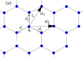
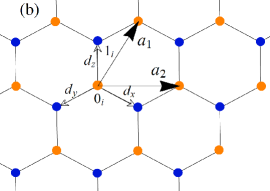
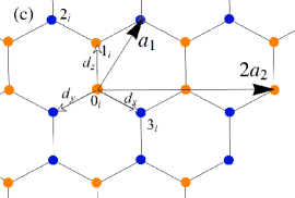
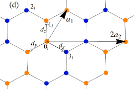
Figure 1: Four possible magnetic configurations: (a) FM ordering; (b) AF Néel order; (c) AF stripy order; (d) AF zigzag order. Red and blue circles correspond to up and down spins. Here $\bm{a}_{1}\!=\!(\!\frac{\sqrt{3}}{2}\hat{x}+\frac{3}{2}\hat{y}\!)$ and $\bm{a}_{2}\!=\!\sqrt{3}\hat{x}$ are two primitive translations. The bond vectors are $\bm{d}_{x}\!=\!(\!\frac{\sqrt{3}}{2}\hat{x}-\frac{1}{2}\hat{y}\!)$, $\bm{d}_{y}\!=\!(\!-\frac{\sqrt{3}}{2}\hat{x}-\frac{1}{2}\hat{y}\!)$ and $\bm{d}_{z}\!=\!\hat{y}$.

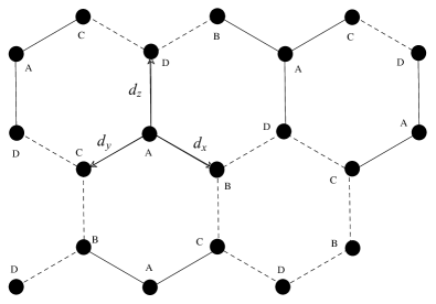
Figure 2: A, B, C and D designate the four sublattices of the Klein transformation. Solid and dashed bonds shows the change of the sign of the $\Gamma$ interaction in the four-sublattice transformation: $\Gamma$ picks up a negative sign on the solid bonds but keeps the sign from unrotated reference frame on the dashed bonds.

II Order by disorder in the extended nearest neighbor Kitaev-Heisenberg model

The Kitaev-Heisenberg model on the honeycomb lattice reads jackeli13

$$H = \sum_{\langle ij\rangle_{\alpha}}\sum_{\gamma}J^{\alpha\gamma}S_{0,i}^{\gamma}S_{1,j}^{\gamma},$$ (1)

where $J^{\alpha\gamma}=J+K\delta_{\alpha,\gamma}$ is the interaction between $\gamma$-component of the pseudospin $S^{\gamma}_{\nu,j}=1/2$, on sublattices $\nu=0,1$. Hereafter, we call these pseudospins simply spins. $J$ and $K$ correspond to the Heisenberg and Kitaev interactions, which in the extended model can be both AF and FM. $\gamma=x,y,z$ denote the spin components in the global reference frame.

The classical phase diagram of the model (1) contains four magnetic phases:jackeli13 ; price13 the ferromagnetic phase (Fig. 1 (a)), the Néel antiferromagnet (Fig. 1(b)), the stripy antiferromagnet (Fig. 1 (c)) and the zigzag antiferromagnet (Fig. 1 (d)). The latter two magnetic states have a four sublattice structure.

All these phases have macroscopic classical degeneracy. While the classical degeneracy of the simple FM state and of the AF Néel state comes straightforwardly from the infinite number of degenerate collinear states, the macroscopic degeneracy of the AF stripy and zigzag phases is more complex, and the degenerate ground state manifold consists of six collinear states and a set of non-collinear multi-$Q$ states. In Appendix A we discuss this question in detail and show that using the four-sublattice Klein transformation for the stripy and the zigzag AF states,jackeli10 ; kimchi14 ; chaloupka15 the nature of the classical degeneracy of all four magnetically ordered states can be understood in a similar way. Importantly, in all cases, the classical degeneracy is accidental and is removed by the order by disorder mechanism which selects a set of collinear states, each with a particular direction of the order parameter.

Following Chaloupka et al,jackeli10 we introduce four auxiliary sublattices A, B, C and D (see Fig.2), fix the direction of the spins on the sublattice A and rotate the spins on the subllatices B, C, and D such that the component of spin corresponding to the bond direction ($x$ for B, $y$ for C and $z$ for D) stays the same but two other spin components change sign. This results in the transformed Hamiltonian with the same form as (1) but with transformed couplings.

Here we consider the Kitaev-Heisenberg model in the full parameter space. For the parameters of the model for which either stripy or zigzag are the ground states, we perform four-sublattice transformation and treat the model (1) in the rotated basis, in which the stripy order maps to the FM and the zigzag order maps to the simple two-sublattice AFM Néel state.

Next, using a Hubbard-Stratonovich transformation of the partition function,sizyuk15 ; peter15 we discuss how the preferred directions of the order parameter in all these phases are selected by thermal below the ordering temperature.

The partition function of the system of classical spins is given by the integral over the Boltzmann weights of the configurations

$$Z=\int\int\left[d\mathbf{S}_{0,i}][d\mathbf{S}_{1,j}\right]\delta(\mathbf{S}_{0,i}^{2}-1)\delta(\mathbf{S}_{1,j}^{2}-1)$$

$$\exp\left[-\beta\sum_{\langle ij\rangle_{\alpha}}\sum_{\gamma}J^{\alpha\gamma}S_{0,i}^{\gamma}S_{1,j}^{\gamma}\right],$$ (2)

where $\mathbf{S}_{0,j}$ and $\mathbf{S}_{1,j}$ are classical spins on sublattices $0$ and $1$, and $\beta=1/(k_{B}T)$ is the inverse temperature. Similarly in the case of a quantum system the partition function is a trace of the Boltzman weights over the spin operators, $Z=Tr\left[\exp\left(-\beta\sum_{\langle ij\rangle_{\alpha}}\sum_{\gamma}J^{\alpha\gamma}S_{0,i}^{\gamma}S_{1,j}^{\gamma}\right)\right]$.

It is more convenient to perform the Hubbard-Stratonovich transformation by representing the Hamiltonian matrix in the basis of the eigenfunctions of the exchange matrix, which can be easily obtained in the momentum space. To this end, we first introduce a six-component vector ${\bm{S}}_{\bm{q}}=(S_{0,{\bm{q}}}^{x},S_{0,{\bm{q}}}^{y},S_{0,{\bm{q}}}^{z},S_{1,{\bm{q}}}^{x},S_{1,{\bm{q}}}^{y},S_{1,{\bm{q}}}^{z})$, with the components given by the Fourier transforms of the $x,y,z$ components of the spins on $0-$ and $1-$sublattices, correspondingly. This allows us to write the Hamiltonian matrix in the momentum space as

$$H=\sum_{\bm{q}}{\bm{S}}_{\bm{q}}^{\dagger}\cdot{\hat{J}}_{\bm{q}}\cdot{\bm{S}}_{\bm{q}},$$ (3)

where the $6\times 6$ exchange matrix ${\hat{J}}_{\bm{q}}$ is defined as

$${\hat{J}}_{\bm{q}}=\left(\begin{array}[]{cccccc}0&0&0&J_{\bm{q}}^{x}&0&0\\ 0&0&0&0&J_{\bm{q}}^{y}&0\\ 0&0&0&0&0&J_{\bm{q}}^{z}\\ \left(J_{\bm{q}}^{x}\right)^{\ast}&0&0&0&0&0\\ 0&\left(J_{\bm{q}}^{y}\right)^{\ast}&0&0&0&0\\ 0&0&\left(J_{\bm{q}}^{z}\right)^{\ast}&0&0&0\end{array}\right),$$ (10)

with matrix elements given by

$$J_{\bm{q}}^{\gamma}=\sum_{\alpha=x,y,z}\left[J+K\delta_{\alpha,\gamma}\right]e^{\imath{\bm{q}}\cdot({\bm{d}}_{\alpha}-{\bm{d}}_{z})}=J_{{\bm{q}}}+K_{\bm{q}}^{\gamma}.$$ (11)

Here we drop the overall phase factor $e^{\imath{\bm{q}}\cdot{\bm{d}}_{z}}=e^{\imath{\bm{q}}\cdot(0,1)}=e^{\imath q_{y}}$ and denote $J_{{\bm{q}}}=J(1+e^{-\imath{\bm{q}}\cdot{\bm{a}}_{1}}+e^{-\imath{\bm{q}}\cdot{\bm{a}}_{2}})$, $K_{\bm{q}}^{\gamma}=Ke^{\imath{\bm{q}}\cdot({\bm{d}}_{\gamma}-{\bm{d}}_{z})}$, where $\bm{a}_{1}\!=\!(\!\frac{\sqrt{3}}{2}\hat{x}+\frac{3}{2}\hat{y}\!)$ and $\bm{a}_{2}\!=\!\sqrt{3}\vec{x}$ are the lattice vectors. The matrix ${\hat{J}}_{\bm{q}}$ is then diagonalized by a unitary transformation, ${\hat{\kappa}}_{\bm{q}}=U^{-1}_{\bm{q}}{\hat{J}}_{\bm{q}}U_{\bm{q}}$, leading to the following form of the Hamiltonian

$$H=\sum_{\bm{q},\nu}\kappa_{{\bm{q}},\nu}{\tilde{S}}^{*}_{{\bm{q}},\nu}{\tilde{S}}_{{\bm{q}},\nu},$$ (12)

where the normal amplitudes of spin-like variables are defined as

$${\tilde{S}}^{\nu}_{\bm{q}}=U_{{\bm{q}},\nu\eta}S^{\eta}_{\bm{q}}.$$ (13)

Note that, depending on the form of the interaction matrix, this transformation in general will mix the spin operators on different sites of the unit cell as well as different components of the spin. However, in the case of the Kitaev-Heisenberg model, while the two sublattices of the honeycomb lattice are mixed, the $x$, $y$, and $z$ components stay separate. The partition function (II) then looks like:

$$Z=\int\int\left[d\mathbf{S}_{0,j}][d\mathbf{S}_{1,j+{\bm{d}}_{z}}\right]\delta(\mathbf{S}_{0,j}^{2}-1)\delta(\mathbf{S}_{1,j+{\bm{d}}_{z}}^{2}-1)$$

$$\exp\left[-\beta\sum_{\bm{q},\nu}\kappa_{{\bm{q}},\nu}{\tilde{S}}^{*}_{{\bm{q}},\nu}{\tilde{S}}_{{\bm{q}},\nu}\right].$$ (14)

Following the steps outlined in Refs.sizyuk15 ; peter15 , we can separate the mean-field and the fluctuational contributions to the partition function, $Z=Z_{\rm MF}Z_{\rm fluct}$. In the Gaussian approximation, the fluctuation part of the partition function,

$$Z_{\mathrm{fluct}}=\int[d\varphi]\exp\left[-\beta{\mathcal{S}}_{\mathrm{fluct}}\right],$$ (15)

where ${\mathcal{S}}_{\mathrm{fluct}}=\sum_{\mathbf{q};\nu,\nu^{\prime}}A_{\mathbf{q,}\nu\nu^{\prime}}\delta\varphi_{\mathbf{q},\nu}^{\mathrm{\ast}}\delta\varphi_{\mathbf{q},\nu^{\prime}}^{\mathrm{}}$ can be obtained by integration over the fluctuation amplitudes $\delta\varphi_{\mathbf{q},\nu}$. The explicit expression for the matrix elements of the fluctuation matrix ${\hat{A}}_{\mathbf{q}}$ computed for an orientation of the mean-field order parameter along arbitrary direction $(\sin\theta\cos\phi,\sin\theta\sin\phi,\cos\theta)$ are given in Appendix B.

Now, the fluctuation contribution to the free energy can be written as

$${\mathcal{F}}_{\rm fluct}=-\frac{1}{\beta}\ln Z_{\rm fluct}=\frac{1}{2\beta}\sum_{\mathbf{q}}\ln\left|\det\{A_{\mathbf{q},\nu\nu^{\prime}}\}\right|.$$ (16)

While the mean-field part of the free energy has the full rotational symmetry, its fluctuational part, ${\mathcal{F}}_{\rm fluct}$, is sensitive to the direction of the mean-field order parameter. Thus, by finding the minima of the fluctuational part of the free energy, we can pin the spontaneous magnetization along some preferred direction of the lattice.

Fig.3 (a) shows the angular dependence of fluctuational free energy ${\mathcal{F}}_{\rm fluct}(\theta,\phi)$ computed for representative parameters $J=-2.9$ meV and $K=8.1$ meV, at which the ground state order is the AF zigzag. The magnitude of ${\mathcal{F}}_{\rm fluct}(\theta,\phi)$ is presented as a color-coded plot on the unit sphere, where the minima and maxima of the free energy are shown by the deep blue and red colors, correspondingly. We see that the minima of ${\mathcal{F}}_{\rm fluct}(\theta,\phi)$ are achieved when the magnetization is directed along one of the cubic axes.

This finding shows that the contribution of the fluctuations to the free energy removes the degeneracy of the ground state found on the mean field level. The states which are selected by the thermal fluctuations are the collinear states with the order parameter pointing along one of the cubic axes, thus confirming previous results of the Monte Carlo simulationsprice12 ; price13 ; sela14 and spin wave analysis by Chaloupka et al.jackeli10

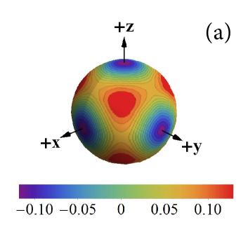
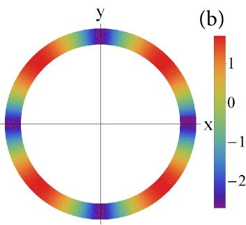
Figure 3: Fluctuational corrections to the free energy in (a) nearest neighbor Kitaev-Heisenberg model computed with $J=-2.9$ meV and $K=8.1$ meV and (b) $J_{1}-K_{1}-J_{2}-K_{2}-J_{3}$ model computed with $J_{1}=5$ meV, $K_{1}=-17$ meV, $J_{2}=-4$ meV, $K_{2}=8$ meV, and $J_{3}=1$ meV.

We discuss the relevance of our findings for the nearest neighbor Kitaev-Heisenberg model for $\alpha-$RuCl₃ in Sec. IV. However in the next section, we will first consider the selection of the direction of the order parameter in the extensions of the Kitaev-Heisenberg model relevant for Na₂IrO₃.

III Order by disorder in $J_{1}-K_{1}-J_{2}-K_{2}-J_{3}$ model

Despite extensive efforts, no consensus concerning the minimal model for Na₂IrO₃ has been reached yet. The most natural extension of the Kitaev-Heisenberg model with ferromagnetic Kitaev interaction which captures the zigzag magnetic order can be obtained by inclusion of farther neighbor couplings. In Na₂IrO₃, these couplings might not be negligible due to the extended nature of the $5d$-orbitals of the Ir ions. In the early works suggesting this possible extension,kimchi11 ; choi12 second and third neighbor couplings were taken into account phenomenologically and only the isotropic part of these interactions was included. The importance of additional nearest neighbor $C_{3}$-symmetric anisotropic terms ($\Gamma$-terms)rau14 ; chaloupka15 or of the spatial anisotropy of the nearest neighbor Kitaev interactions,yamaji14 were also discussed in the literature as a possible source for the stabilization of the zigzag phase.

Here we consider the $J_{1}-K_{1}-J_{2}-K_{2}-J_{3}$ model,sizyuk14 which still has the same symmetry as the original Kitaev-Heisenberg model but contains Kitaev interactions between both nearest and second nearest neighbors. The model reads

$$\mathcal{H}=J_{1}\sum_{\langle i,j\rangle_{\gamma}}{\bf S}_{i}{\bf S}_{j}+K_{1}\sum_{\langle i,j\rangle_{\gamma}}S_{j}^{\gamma}S_{j}^{\gamma}+$$ (17)

$$J_{2}\sum_{\langle\langle i,j\rangle\rangle_{\tilde{\gamma}}}{\bf S}_{i}{\bf S}_{j}+K_{2}\sum_{\langle\langle i,j\rangle\rangle_{\tilde{\gamma}}}S_{i}^{\tilde{\gamma}}S_{j}^{\tilde{\gamma}}+J_{3}\sum_{\langle\langle\langle i,j\rangle\rangle\rangle}{\bf S}_{i}{\bf S}_{j},$$

where $J_{1}>0$, $K_{1}<0$, $J_{2}<0$, $K_{2}>0$, and $J_{3}>0$; $\langle\,\rangle$, $\langle\langle\,\rangle\rangle$ and $\langle\langle\langle\,\rangle\rangle\rangle$ denote nearest neighbor, second nearest neighbor and third nearest neighbor, respectively. $\gamma=x,y,z$ and $\tilde{\gamma}={\tilde{x}},{\tilde{y}},{\tilde{z}}$ denote the three types of nearest neighbor and second nearest neighbor bonds of the honeycomb lattice, respectively. It is important to note that the second neighbor Kitaev interactions do not change the space group symmetries of the original Kitaev-Heisenberg model.

For realistic sets of the parameters describing Na₂IrO₃, the second neighbor Kitaev interaction, $K_{2}$, computed from the microscopic approach based on the ab-initio calculation by Foevtsova et al,katerina13 ; note appeared to be the largest interaction after the nearest neighbor Kitaev interaction, $K_{1}$, and turn out to be antiferromagnetic. The mechanism behind the large magnitude of $K_{2}$ in Na₂IrO₃ is physically very clear: It originates from the large diffusive Na ions that reside in the middle of the exchange pathways, and the constructive interference of a large number of pathways. Moreover, the $K_{1}$-$K_{2}$ model, that only includes Kitaev interactions,ioannis15 already stabilizes the zigzag phase for the proper signs of $K_{1}$ and $K_{2}$. However, as we have discussed in Ref.ioannis15 , the $K_{1}$-$K_{2}$ model is still not sufficient to comply with all available experimental data.

The classical degeneracy of the zigzag state obtained within the $J_{1}-K_{1}-J_{2}-K_{2}-J_{3}$ model with FM $K_{1}$ is different from the one of the zigzag state realized in the extended Kitaev-Heisenberg model with AFM $K_{1}$ interaction. To see what difference the sign of $K_{1}$ makes, let us consider the zigzag pattern in Fig.1 (d). With AFM $K_{1}$, the pattern, that minimizes the classical energy in the zigzag state with ferromagnegnetic $y$ and $z$ bonds, has the spins pointing along the $x-$axis to take advantage of the Kitaev interaction on the AFM $x$-bonds. On the other hand the same pattern with FM $K_{1}$ takes advantage of the Kitaev interaction on the FM $y-$ and $z-$ bonds by putting spins in the $yz-$plane. Thus the degenerate ground state manifold for a given zigzag pattern with FM $K_{1}$ is one of $xy-$, $yz-$, or $zx-$ planes. Furthermore, when the Klein duality 4-sublattice transformationjackeli10 is applied to the $J_{1}-K_{1}-J_{2}-K_{2}-J_{3}$ zigzags, these states do not turn into Néel AFM state, and instead turn into non-collinear states, that are more difficult to work with than the original zigzag states. Working with the zigzag states directly increases the magnetic unit cell to 4 sites, labeled in Fig 1(d).

The Hamiltonian matrix in the momentum space can be again written in the form of Eq. (3), however this time due to the larger unit cell the exchange matrix ${\hat{J}}_{\bm{q}}$ is $12\times 12$, instead of $6\times 6$. Its matrix elements are given in Appendix C. The fluctuations matrix $A_{\mathbf{q,}\nu\nu^{\prime}}$ is calculated as before according to equation (24), with the constraint matrix $C_{{\bm{q}},\mu,\mu^{\prime}}$ of equation (32) now containing 4 identical blocks instead of 2. The fluctuation matrix again contains the information on the direction of the spins and transmits this information to the free energy corrections that we plot in Fig. 3(b). Since the spins are confined to a plane for a given zigzag state we have only the angle of the direction of spins in that plane. The color of the band at a given angle then gives the size of the fluctuational correction to the free energy, with violet being lowest and red highest energy states. We see that again the Kitaev anisotropies prefer to align the magnetization along the cubic axes. Note, however, that unlike the extended KH model, where there were 6 equivalent states, here there are 4 directions for each of the three zigzag patterns, giving a total of 12 states.

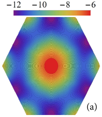
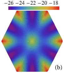
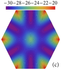
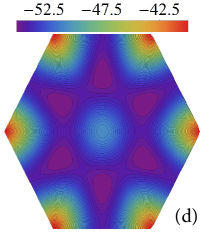
Figure 4: The lowest eigenvalue of the $J_{1}-K_{1}-J_{2}-K_{2}-J_{3}-\Gamma_{1}$ model obtained with the Luttinger-Tisza method is shown on the first Brillouin zone. We use $J_{1}=3$ meV, $K_{1}=-17$ meV, $J_{2}=-3$ meV, $K_{2}=6$ meV, $J_{3}=1$ meV, and (a) $\Gamma_{1}=1$ meV, (b) $\Gamma_{1}=20$ meV, (c) $\Gamma_{1}=25$ meV, and (d) $\Gamma_{1}=50$ meV.

IV The role of off-diagonal symmetric $\Gamma$-term.

IV.1 Directions of the ordered moments in Na₂IrO₃.

The discussion above has clearly shown, that neither the original Kitaev model nor the extended $J_{1}-K_{1}-J_{2}-K_{2}-J_{3}$ model can correctly explain the experimental data in Na₂IrO₃. Since the easy axes directions are determined solely by the anisotropy terms, only the inclusion of other types of the anisotropies can improve the situation. Here we consider the off-diagonal symmetric $\Gamma$-terms. The role of these terms in the nearest-neighbor Kitaev model has been studied in Refs.rau14 ; chaloupka15 . These studies have shown that the small $\Gamma$-terms do not immediately destabilize the zigzag phase, but lead to a deviation of the magnetic moments from the cubic axes.

The origin of $\Gamma$-terms can be easily seen from the most general form of the bilinear exchange coupling matrix, which on the bond $(i,j)$ has the form given by

$$\Xi_{i,j}=\left(\begin{array}[]{ccc}J^{xx}&J^{xy}&J^{xz}\\ J^{yx}&J^{yy}&J^{yz}\\ J^{zx}&J^{zy}&J^{zz}\\ \end{array}\right).$$ (21)

While the Kitaev term comes from the anisotropy of the diagonal matrix elements of $\Xi_{i,j}$, e.g. $K_{1}=J_{1}^{zz}-J_{1}^{xx}$, the symmetric and antisymmetric combinations of off-diagonal elements represent other types of possible bond-anisotropies. In the absence of the trigonal distortion, the inversion symmetry prohibits the existence of antisymmetric interactions but some of the symmetric combinations are allowed, i.e. on a given $\gamma$-bond, the interaction between the other two spin components, $\Gamma^{\gamma}(S_{i}^{\alpha}S_{j}^{\beta}+S_{i}^{\beta}S_{j}^{\alpha})$, where $\Gamma^{\gamma}=\frac{1}{2}(J_{1}^{\alpha\beta}+J_{1}^{\beta\alpha})$, is non-zero. Our previous resultssizyuk14 suggest that in Na₂IrO₃ the magnitude of the strength of $\Gamma$ on the nearest neighbor bonds is about 2-3 meV and vanishes for the second neighbors.

Here we consider the $J_{1}-K_{1}-J_{2}-K_{2}-J_{3}-\Gamma$ model with the previous choice of Heisenberg and Kitaev interactions and treat $\Gamma$ as a free parameter. A straightforward classical minimization in momentum space using Luttinger-Tisza approachLuttinger46 ; Litvin74 ; kaplan07 shows that up to very large values of $\Gamma\sim 20$ meV the minima of the classical energy are located at the $M$ points corresponding to the zigzag states. This is clearly seen in Fig. 4(a) where we plot the lowest eigenvalues obtained for $\Gamma=1$ meV. At larger values of $\Gamma$, the minima shift along the lines connecting $M$ points and the center of the Brillouin zone (see Fig. 4 (b) for $\Gamma=20$ meV), indicating the transition to incommensurate order. The incommensurability of the Luttinger-Tisza solution increases further with larger values of $\Gamma$, which is shown in Figs. 4 (c) and (d). The exact value of $\Gamma$ at which the transition occurs is difficult to determine due to the transition being so smooth, Note, however, that the transition occurs at values of $\Gamma$ far beyond those predicted from our microscopic calculations at ambient pressure.sizyuk14

After we have demonstrated that adding small $\Gamma$ interactions to the $J_{1}-K_{1}-J_{2}-K_{2}-J_{3}$ model does not destabilize the zigzag order, let us now show that in the presence of $\Gamma$ the mean-field degeneracy is already lifted and the preferred directions of the order parameter are selected. This is clearly seen in Fig. 5 (a) and (b), where the mean field energy of the zigzag order is computed for $\Gamma=1$ meV and $\Gamma=-1$ meV, respectively. By inspection, we can see that non-zero $\Gamma$ selects the face diagonals as easy axes for magnetic ordering, and the sign of $\Gamma$ determines which of the two face diagonals are preferred. For concreteness, let us consider the zigzag with AFM $z-$bonds. As we discussed above the case for $\Gamma=0$, the easy $xy$-plane is selected at the mean-field level of the $J_{1}-K_{1}-J_{2}-K_{2}-J_{3}$ model. Then, the inclusion of positive $\Gamma$ interaction on $x$ and $y$ bonds gives zero contribution to the energy since on these bonds it involves the spin component perpendicular to the easy plane, but it gives maximal lowering of the energy on the $z$-bonds if the spins point along $[110]$ and $[{\bar{1}}{\bar{1}}0]$, $[{\bar{1}}10]$ and $[{\bar{1}}10]$ directions correspondingly for positive and negative values of $\Gamma$. The estimate for the smallest $\Gamma$, at which the selection of face diagonals takes place, can be done by comparing the mean-field energy gain due to $\Gamma$ with the energy gain due to fluctuations at $\Gamma=0$, which at $T=0$ is equal to the zero point energy and is a function of $K_{1}$ and $K_{2}$. At finite temperature, the contribution to the energy from the Gaussian fluctuations at each $T$ can be computed by our method, and this energy will give the lower bound for the magnitude of $\Gamma$ needed to change the orientation of magnetic order from the cubic to the face diagonal.

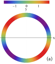
Figure 5: Mean field energy of the zigzag orders in $J_{1}-K_{1}-J_{2}-K_{2}-J_{3}$ model with the contribution of (a) $\Gamma=1$ meV and (b) $\Gamma=-1$ meV.

IV.2 Directions of the ordered moments in $\alpha-$RuCl₃.

The microscopic calculations for $\alpha-$RuCl₃ emphasized the importance of the off-diagonal nearest neighbor $\Gamma$ interactions.kee15 The effect of adding $\Gamma$ interaction to the nearest neighbor Kitaev-Heisenberg model is easiest to understand in the rotated reference frame of the four-sublattice Klein transformation.chaloupka15 ; kimchi14 The Kitaev and Heisenberg interactions do not change their form and only change the value of the coupling constants under this transformation. On the other hand, $\Gamma$-interaction picks up a bond dependent sign as shown in Fig. 2. In fact, $\Gamma$ changes the sign on half of the bonds, i.e. there are just as many negative bonds as there are positive bonds for each Kitaev type of bonds. Since the Klein transformed version of the zigzag state is the AFM Néel state, all the bonds are AFM and involve the same pair of spins. Thus the contribution of the $\Gamma$ interaction to the mean-field energy cancels out, and the set of states remains degenerate. This means that as long as we remain in the small window where $\Gamma$ does not destabilize the zigzag order found by Rau et al.,rau14 we can perform our order-by-disorder approach to see what state is chosen.

Figs.6 (a)-(c) show the fluctuation free energy computed for the $J-K-\Gamma$ model for $J_{1}=-2.9$ meV and $K_{1}=8.1$ meV, suggested by Banerjee et al.,banerjee15 and $\Gamma=0.7$ meV, 0.8 meV and 0.9 meV, respectively. In Fig. 6 (a), $\Gamma=0.7$ meV, the minima of the fluctuational free energy are still along cubic directions. For larger $\Gamma$-interaction, the system prefers the states with at least two nonzero spin components and, therefore, the transition towards [111] preferred directions of the order parameter takes place. This is shown in Fig. 6 (b) and (c), in which the fluctuational energy is plotted for $\Gamma=0.8$ meV and 0.9 meV. While in Fig. 6 (b) only very shallow minima are seen along [111] directions, in Fig. 6 (c) both the pronounced minima along the cubic body diagonals and maxima along the cubic axes are very clearly seen. Remember that the computation is done in the rotated reference frame. Therefore, only the states with the orientation of the order parameter along the cubic axes will give the collinear states in the unrotated reference frame. The states with order parameter pointing along [111] directions in the rotated reference frame correspond to non-collinear states in the unrotated reference frame. Since recent experiments by Cao et al.cao16 have established that spins point along a cubic axis, by calculating the fluctuational corrections as a function of $\Gamma$, we can find an upper bound on its value, such that the Kitaev fluctuations dominate and keep the cubic axes as the preferred directions. From our calculations it follows that for $J_{1}=-2.9$ meV and $K_{1}=8.1$ meV the upper bound for $\Gamma$ is about 0.8 meV. Finally, for this set of parameters the transition to the 120^∘- AFM order occurs around $\Gamma=1.6$ meV. Note that this estimate is far smaller than the $\Gamma$ values resulting from ab initio calculations.kee15 .

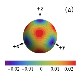
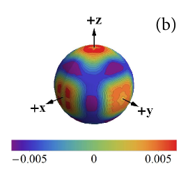
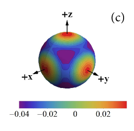
Figure 6: (Color online) Fluctuational corrections to the free energy in the nearest neighbor Kitaev Heisenberg model with $\Gamma$ interaction. We used the following parameters: $J=-2.9$ meV, $K=8.1$ meV and (a) $\Gamma=0.7$ meV, (b) $\Gamma=0.8$ meV, and (c) $\Gamma=0.9$ meV. The minima of the free energy are shown by deep blue color and the maxima by intense red color.

V Concluding remarks

In this paper we explored how the direction of the magnetic moments in the zigzag ground state order is chosen in Na₂IrO₃ and $\alpha-$RuCl₃. In both compounds, the Kitaev interaction plays an important role. For the case of FM nearest neighbor Kitaev interaction, like in Na₂IrO₃, farther neighbor interactions are essential for stabilizing the zigzag ground state. For the AFM nearest neighbor Kitaev interaction, which was widely suggested to be the dominant interaction in $\alpha-$RuCl₃,sears15 ; johnson15 ; banerjee15 ; cao16 ; kee15 the zigzag order can be stabilized already within the nearest neighbor model.

We proposed that the $J_{1}-K_{1}-J_{2}-K_{2}-J_{3}-\Gamma$ model can explain all the experimental finding in Na₂IrO₃. In this model the selection of the experimentally observed face diagonal direction of the order parameter happens already on the mean-field level due to the small bond-dependent anisotropic term $\Gamma$.

In $\alpha-$RuCl₃, if the the nearest neighbor Kitaev interaction is AFM, the original Kitaev-Heisenberg modeljackeli13 is sufficient to explain both the collinear zigzag ground state and the cubic directions of the order parameter. We studied the effect of the $\Gamma$-term and showed that while on the mean-field level it doesn’t affect the ground state degeneracy, it favors non-collinear 3-Q states, instead of the experimentally observed zigzag state with spins along cubic axes, once the Gaussian fluctuations are included. Thus, it appears to be an upper bound for $\Gamma$-term, which can be estimated for a given set of nearest neighbor parameters.

After the completion of our paper, we became aware of an independent study by Winter et al. roser16 of the magnetic interactions in the Kitaev materials Na₂IrO₃ and $\alpha-$RuCl₃. In this work, the authors treated all interactions up to third neighbours on equal footing by combining exact diagonalization and ab-initio techniques. One of the main findings of this work is that the third neighbor Heisenberg interaction is important in all Kitaev materials.

Let us briefly compare the results of Ref. roser16 with our findings. The conclusions of the authors of Ref. roser16 about the ordering in Na₂IrO₃ are in agreement with our findings, despite the fact that their estimates for $K_{2}$ suggest significantly smaller values than the ones that we obtained by including only the dominant superexchange processes between the second neighbors. The agreement holds because the second neighbor Kitaev interaction $K_{2}$ and the third neighbor interaction $J_{3}$ favor the same type of AFM zigzag ground state.

For $\alpha-$RuCl₃, the authors of Ref.roser16 suggest (i) that there may be possible variations of in-plane interactions due to lattice distortions, and (ii) that the nearest neighbor Kitaev interaction may be FM and the third neighbor coupling $J_{3}$ may be large and AFM. The FM sign of the nearest neighbor Kitaev interaction was also suggested by Yadav et al in Ref.hozoi16 . If this is indeed the case, the physics of $\alpha-$RuCl₃ is similar to that of Na₂IrO₃. This, however, still needs to be verified by a detailed comparison with the experimental data.

Acknowledgements. We acknowledge insightful discussions with C. Batista, G. Jackeli, M.Garst, G. Khaliullin and I. Rousochatzakis. N.P. and Y.S. acknowledge the support from NSF Grant DMR-1511768. N.P. acknowledges the hospitality of KITP and partial support by the National Science Foundation under Grant No. NSF PHY11-25915.

Appendix A The classical degeneracy of the extended Kitaev-Heisenberg model

In this Appendix we provide detailed discussion of the classical degeneracy of the extended Kitaev-Heisenberg model at parameters for which either the stripy or the zigzag AF phases are realized as the ground state and the manifold of classically degenerate states is rather complex.

To be specific, let us first consider the stripy phase. It contains six inequivalent collinear stripy states with FM bonds along either Kitaev $x-$, $y-$ or $z-$bonds. It also contains infinite number of non-collinear (coplanar and non-coplanar) states. The spin order in the $x-$, $y-$ or $z-$ stripy states can be described either with a help of four magnetic sublattices or by a simple spiral characterized by a single-$Q$ wave vector: ${\mathbf{Q}}_{x}=(\pi/\sqrt{3},\pi)$, ${\mathbf{Q}}_{y}=(\pi/\sqrt{3},-\pi)$ and ${\mathbf{Q}}_{z}=(-2\pi/\sqrt{3},0)$. One of the stripy states with FM $z$-bonds is shown in Fig.1 (c). In each of these stripy states the spins are aligned along one of the cubic directions which is locked to the spatial orientation of a stripy pattern by the Kitaev interaction, i.e. the direction of the order parameter is defined by the wave vector ${\mathbf{Q}}={\mathbf{Q}}_{x},{\mathbf{Q}}_{y}$ or ${\mathbf{Q}}_{z}$ determining the breaking of the translation symmetry.

The structure of the manifold of the non-collinear states, which looks rather complex in the original model, can be easily understood with the help of the four-sublattice transformation (see Fig.2) based on the Klein duality.jackeli10 ; chaloupka15 ; kimchi14 In the new rotated basis, the stripy phase is mapped to the FM order with a unique ordering vector ${\mathbf{Q}}=0$. Classically, all states with arbitrary direction of the FM order have the same energy. FM states with order parameter along the cubic axes give the six stripy phases in the unrotated spin basis discussed above. Arbitrary directions of the FM order parameter lead to a set of non-coplanar states in which each component of spin, $S_{x}$, $S_{y}$, and $S_{z}$, transforms with its own ${\mathbf{Q}}_{x}$, ${\mathbf{Q}}_{y}$ and ${\mathbf{Q}}_{z}$ wavevector, which coincide with the ${\mathbf{Q}}$ vectors describing the spatial orientation of the stripes in the respective collinear states.

Using these three ordering vectors, we can write the non-coplanar phase of the unrotated spins as

$${\mathbf{S}}_{i,0}=(s_{\theta}c_{\phi}\,e^{\imath{\mathbf{Q}}_{x}\cdot{\bm{R}}_{i}},s_{\theta}s_{\phi}\,e^{\imath{\mathbf{Q}}_{y}\cdot{\bm{R}}_{i}},c_{\theta}\,e^{\imath{\mathbf{Q}}_{z}\cdot{\bm{R}}_{i}}),$$ (22)

where $\theta$ and $\phi$ are the polar and azimuthal angles of the FM order parameter. ${\mathbf{S}}_{i,0}$ denote the spins on the sublattice $0$ and the spins on the sublattice $1$ are obtained from ${\mathbf{S}}_{i,0}$ by a constant phase shift coming from the spin rotation on that bond as prescribed by the four sublattice transformation. As in Fig.1 (c), the sublattices 0 and 1 are connected by the $z$ bond, the order of the spins on the subllatice 1 is given by

$${\mathbf{S}}_{i,1}=(S_{i,0}^{x}\,e^{\imath\pi},\,S_{i,0}^{y}\,e^{\imath\pi},S_{i,0}^{z})$$ (23)

In the zigzag phase, the structure of the classical states manifold is very similar to the stripy phase. The four-sublattice transformation maps the zigzag phase onto the Néel AF phase. The generic state is again described by the three-${\mathbf{Q}}$ spiral state. The only difference is that the spins on sublattice 1 have an overall phase factor of $\pi$, ${\mathbf{S}}_{i,1}=(S_{i,0}^{x},\,S_{i,0}^{y},\,S_{i,0}^{z}e^{\imath\pi})$.

Appendix B The matrix elements $A_{\mathbf{q,}\nu\nu^{\prime}}$ computed for the KH model.

The matrix elements $A_{\mathbf{q,}\nu\nu^{\prime}}$ can be written as

$$A_{\mathbf{q,}\nu\nu^{\prime}}=\frac{\delta_{\nu,\nu^{\prime}}}{\kappa_{{\bm{q}},\nu}}+s(\kappa_{{\bm{q}},\nu})s(\kappa_{{\bm{q}},\nu^{\prime}})U^{-1}_{{\bm{q}},\nu,\mu}C_{{\bm{q}},\mu,\mu^{\prime}}U_{{\bm{q}},\nu,\mu},$$ (24)

where a repeated index implies a summation over. The first term in (24) is the contribution from the interaction term and the second term is from the constraint term.sizyuk15 ; peter15 For convenience, the constraint matrix ${\hat{C}}_{{\bm{q}}}$ can be first written in the original basis, in which the interaction term is not diagonal, and then transformed to the eigenbasis of the Hamiltonian with a help of the unitary transformation $U_{\bm{q}}$. In the original basis the constraint matrix ${\hat{C}}_{{\bm{q}}}$ consists of two blocks, one for each sublattice. The A-sublattice block has elements $C_{{\bm{q}},\mu,\mu^{\prime}}$ with $\mu,\mu^{\prime}=1,2,3$ and the B-sublattice block has the elements with $\mu,\mu^{\prime}=4,5,6$. The two blocks are identical, so ${\hat{C}}_{{\bm{q}}}$ takes the following form:

$${\hat{C}}_{\bm{q}}=\left(\begin{array}[]{cccccc}C_{{\bm{q}},11}&C_{{\bm{q}},12}&C_{{\bm{q}},13}&0&0&0\\ C_{{\bm{q}},21}&C_{{\bm{q}},22}&C_{{\bm{q}},23}&0&0&0\\ C_{{\bm{q}},31}&C_{{\bm{q}},32}&C_{{\bm{q}},33}&0&0&0\\ 0&0&0&C_{{\bm{q}},11}&C_{{\bm{q}},12}&C_{{\bm{q}},13}\\ 0&0&0&C_{{\bm{q}},21}&C_{{\bm{q}},22}&C_{{\bm{q}},23}\\ 0&0&0&C_{{\bm{q}},31}&C_{{\bm{q}},32}&C_{{\bm{q}},33}\end{array}\right)$$ (31)

with matrix elements given by

$$\begin{array}[c]{l}C_{{\bm{q}},11}=-\frac{2}{3}\bigl{[}\beta_{c}(1-s_{\theta}^{2}c_{\phi}^{2})+3\beta rs_{\theta}^{2}c_{\phi}^{2}\bigr{]},\\ C_{{\bm{q}},22}=-\frac{2}{3}\bigl{[}\beta_{c}(1-s_{\theta}^{2}s_{\phi}^{2})+3\beta rs_{\theta}^{2}s_{\phi}^{2}\bigr{]},\\ C_{{\bm{q}},33}=-\frac{2}{3}\bigl{[}\beta_{c}s^{2}_{\theta}+3\beta rc^{2}_{\theta}\bigr{]},\\ C_{{\bm{q}},12}=C_{{\bm{q}},21}=-\frac{2}{3}(3\beta r-\beta_{c})s^{2}_{\theta}c_{\phi}s_{\phi},\\ C_{{\bm{q}},13}=C_{{\bm{q}},31}=-\frac{2}{3}(3\beta r-\beta_{c})s_{\theta}s_{\theta}c_{\phi},\\ C_{{\bm{q}},23}=C_{{\bm{q}},32}=-\frac{2}{3}(3\beta r-\beta_{c})s_{\theta}s_{\phi}c_{\phi},\end{array}$$ (32)

where, to shorten notations, we denote $\sin\theta(\phi)\equiv s_{\theta(\phi)}$ and $\cos\theta(\phi)\equiv c_{\theta(\phi)}$.

Appendix C Coupling $J_{\mu,\nu}({\bm{q}})$ of the $J_{1}-K_{1}-J_{2}-K_{2}-J_{3}$ model.

For shortness we define $q_{1}={\bf q}\cdot{\bf a}_{1}$, $q_{2}={\bf q}\cdot{\bf a}_{2}$, and $q_{z}={\bf q}\cdot{\bf d}_{z}$. The diagonal matrix elements for $\mu=1,4,7$ and 10 are equal to $J_{\mu,\mu}({\bm{q}})=(J_{2}+K_{2})\cos q_{1}$, all other diagonal elements are equal to $J_{\mu,\mu}({\bm{q}})=J_{2}\cos q_{1}$. The non-zero off-diagonal elements $J_{\mu,\nu}({\bm{q}})$ for $\nu>\mu$ are

$$J_{1,4}({\bm{q}})=\frac{1}{2}J_{1}(e^{\imath q_{z}}+e^{\imath(-q_{1}+q_{z})})$$

$$J_{2,5}({\bm{q}})=\frac{1}{2}\left(J_{1}(e^{\imath q_{z}}+(J_{1}+K_{1})e^{\imath(-q_{1}+q_{z})})\right)$$

$$J_{3,6}({\bm{q}})=\frac{1}{2}\left((J_{1}+K_{1})(e^{\imath q_{z}}+J_{1}e^{\imath(-q_{1}+q_{z})})\right)$$

$$J_{1,7}({\bm{q}})=J_{2}(\cos(q_{1}-q_{2})+\cos q_{2})$$

$$J_{2,8}({\bm{q}})=(J_{2}+K_{2})\cos(q_{1}-q_{2})+J_{2}\cos q_{2}$$

$$J_{3,9}({\bm{q}})=J_{2}\cos(q_{1}-q_{2})+(J_{2}+K_{2})\cos q_{2}$$

$$J_{1,10}({\bm{q}})=\frac{1}{2}\Big{(}(J_{1}+K_{1})e^{\imath(q_{2}-q_{1}+q_{z})}+\,$$

$$\left.\,\,\,\,\,\,\,\,\,\,\,\,\,J_{3}(e^{\imath(q_{2}+q_{z})}+e^{\imath(q_{2}-2q_{1}+q_{z})}+e^{\imath(-q_{2}+q_{z})})\right)$$

$$J_{2,11}({\bm{q}})=\frac{1}{2}\Big{(}J_{1}e^{\imath(q_{2}-q_{1}+q_{z})}+$$

$$\left.\,\,\,\,\,\,\,\,\,\,\,\,\,J_{3}(e^{\imath(q_{2}+q_{z})}+e^{\imath(q_{2}-2q_{1}+q_{z})}+e^{\imath(-q_{2}+q_{z})})\right)$$

$$J_{3,12}({\bm{q}})=\frac{1}{2}\Big{(}J_{1}e^{\imath(q_{2}-q_{1}+q_{z})}+$$

$$\left.\,\,\,\,\,\,\,\,\,\,\,\,\,J_{3}(e^{\imath(q_{2}+q_{z})}+e^{\imath(q_{2}-2q_{1}+q_{z})}+e^{\imath(-q_{2}+q_{z})})\right)$$

$$J_{4,7}({\bm{q}})=\frac{1}{2}\left((J_{1}+K_{1})e^{\imath(q_{1}-q_{2}-q_{z})}+\right.$$

$$\left.\,\,\,\,\,\,\,\,\,\,\,\,\,J_{3}(e^{\imath(2q_{1}-q_{2}-q_{z})}+e^{\imath(-q_{2}-q_{z})}+e^{\imath(q_{2}-q_{z})})\right)$$

$$J_{5,8}({\bm{q}})=\frac{1}{2}\left(J_{1}e^{\imath(q_{1}-q_{2}-q_{z})}+\right.$$

$$\left.\,\,\,\,\,\,\,\,\,\,\,\,\,J_{3}(e^{\imath(2q_{1}-q_{2}-q_{z})}+e^{\imath(-q_{2}-q_{z})}+e^{\imath(q_{2}-q_{z})})\right)$$

$$J_{6,9}({\bm{q}})=\frac{1}{2}\left(J_{1}e^{\imath(q_{1}-q_{2}-q_{z})}+\right.$$

$$\left.\,\,\,\,\,\,\,\,\,\,\,\,\,J_{3}(e^{\imath(2q_{1}-q_{2}-q_{z})}+e^{\imath(-q_{2}-q_{z})}+e^{\imath(q_{2}-q_{z})})\right)$$

$$J_{4,10}({\bm{q}})=J_{2}\Big{(}\cos q_{2}+\cos(q_{2}-q_{1})\Big{)}$$

$$J_{5,11}({\bm{q}})=J_{2}\cos q_{2}+(J_{2}+K_{2})\cos(q_{2}-q_{1})$$

$$J_{6,12}({\bm{q}})=(J_{2}+K_{2})\cos q_{2}+J_{2}\cos(q_{2}-q_{1})$$

$$J_{7,10}({\bm{q}})=\frac{1}{2}J_{1}(e^{\imath q_{z}}+e^{\imath(-q_{1}+q_{z})})$$

$$J_{8,11}({\bm{q}})=\frac{1}{2}\Big{(}J_{1}e^{\imath q_{z}}+(J_{1}+K_{1})e^{\imath(-q_{1}+q_{z})}\Big{)}$$

$$J_{9,12}({\bm{q}})=\frac{1}{2}\Big{(}(J_{1}+K_{1})e^{\imath q_{z}}+J_{1}e^{\imath(-q_{1}+q_{z})}\Big{)}$$

References

- (1) A. Kitaev, Ann. Phys. 321, 2 (2006).
- (2) G. Khaliullin, Prog. Theor. Phys. Suppl. 160, 155 (2005).
- (3) G. Jackeli and G. Khaliullin, Phys. Rev. Lett. 102, 017205 (2009).
- (4) Z. Nussinov, J. van den Brink, Rev. Mod. Phys. 87 1 (2015).
- (5) Y. Singh and P. Gegenwart, Phys. Rev. B 82, 064412 (2010).
- (6) Y. Singh, S. Manni, J. Reuther, T. Berlijn, R. Thomale, W. Ku, S. Trebst, and P. Gegenwart, Phys. Rev. Lett. 108, 127203 (2012).
- (7) X. Liu, T. Berlijn, W.-G. Yin, W. Ku, A. Tsvelik, Young-June Kim, H. Gretarsson, Y. Singh, P. Gegenwart, and J. P. Hill, Phys. Rev. B 83, 220403 (2011).
- (8) F. Ye, S. Chi, H. Cao, B. C. Chakoumakos, J. A. Fernandez-Baca, R. Custelcean, T. F. Qi, O. B. Korneta, and G. Cao, Phys. Rev. B 85, 180403 (2012).
- (9) S. K. Choi, R. Coldea, A. N. Kolmogorov, T. Lancaster, I. I. Mazin, S. J. Blundell, P. G. Radaelli, Yogesh Singh, P. Gegenwart, K. R. Choi, S.-W. Cheong, P. J. Baker, C. Stock, and J. Taylor, Phys. Rev. Lett. 108, 127204 (2012).
- (10) H. Gretarsson, J. P. Clancy, Yogesh Singh, P. Gegenwart, J. P. Hill, Jungho Kim, M. H. Upton, A. H. Said, D. Casa, T. Gog, and Young-June Kim, Phys. Rev. B 87, 220407(R)
- (11) S. H. Chun, J.-W. Kim, J. Kim, H. Zheng, C. C. Stoumpos, C. D. Malliakas, J. F. Mitchell, Kavita Mehlawat, Yogesh Singh, Y. Choi, T. Gog, A. Al-Zein, M. Moretti Sala, M. Krisch, J. Chaloupka, G. Jackeli, G. Khaliullin, B. J. Kim, Nature Physics 11, 462 (2015).
- (12) K. Modic, T. E. Smidt, I. Kimchi, N. P. Breznay, A. Biffin, S. Choi, R. D. Johnson, R. Coldea, P. Watkins-Curry, G. T. McCandess, et al., Nature communications 5, 4203 (2014).
- (13) A. Biffin, R. D. Johnson, S. Choi, F. Freund, S. Manni, A. Bombardi, P. Manuel, P. Gegenwart, and R. Coldea, Phys. Rev. B 90, 205116 (2014).
- (14) A. Biffin, R.D. Johnson, I. Kimchi, R. Morris, A. Bombardi, J.G. Analytis, A. Vishwanath, and R. Coldea, Phys. Rev. Lett. 113, 197201 (2014).
- (15) T. Takayama, A. Kato, R. Dinnebier, J. Nuss, H. Kono, L.S.I. Veiga, G. Fabbris, D. Haskel, and H. Takagi, Phys. Rev. Lett. 114, 077202 (2015).
- (16) I. Pollini, Phys. Rev. B 53, 12769 (1996).
- (17) K. W. Plumb, J. P. Clancy, L. J. Sandilands, V. V. Shankar, Y. F. Hu, K. S. Burch, H.-Y. Kee, and Y.-J. Kim, Phys. Rev. B 90, 041112 (2014).
- (18) J. A. Sears, M. Songvilay, K. W. Plumb, J. P. Clancy, Y. Qiu, Y. Zhao, D. Parshall, and Young-June Kim, Phys. Rev. B 91, 144420 (2015).
- (19) M. Majumder, M. Schmidt, H. Rosner, A. A. Tsirlin, H. Yasuoka, and M. Baenitz, Phys. Rev. B 91, 180401 (2015).
- (20) R. D. Johnson, S. C. Williams, A. A. Haghighirad, J. Singleton, V. Zapf, P. Manuel, I. I. Mazin, Y. Li, H. O. Jeschke, R. Valenti, and R. Coldea Phys. Rev. B 92, 235119 (2015).
- (21) A. Banerjee, C. Bridges, J.-Q. Yan, A. A. Aczel, L. Li, M. B. Stone, G. E. Granroth, M. D. Lumsden, Y. Yiu, J. Knolle et al., Nature Materials 15, 733-740, (2016).
- (22) H.B. Cao, A. Banerjee, J.-Q. Yan, C.A. Bridges, M.D. Lumsden, D.G. Mandrus, D.A. Tennant, B.C. Chakoumakos, S.E. Nagler, arXiv:1602.08112.
- (23) J. Chaloupka, G. Jackeli, and G. Khaliullin, Phys. Rev. Lett. 105, 027204 (2010).
- (24) J. Chaloupka, G. Jackeli, G. Khaliullin, Phys. Rev. Lett. 110, 097204 (2013).
- (25) V. M. Katukuri, S. Nishimoto, V. Yushankhai, A. Stoyanova, H. Kandpal, S. Choi, R. Coldea, I. Rousochatzakis, L. Hozoi, J. van den Brink, New J. Phys. 16, 013056 (2014).
- (26) Y. Sizyuk, C. Price, P. Wölfle, and N. B. Perkins, Phys. Rev. B 90, 155126 (2014).
- (27) J. Reuther, R. Thomale and S. Rachel, Phys. Rev. B 90, 100405( R) (2014).
- (28) I. Rousochatzakis, J. Reuther, R. Thomale, S. Rachel, and N. B. Perkins, Phys. Rev. X 5 , 5 041035 (2015).
- (29) Heung-Sik Kim, Vijay Shankar V., Andrei Catuneanu, and Hae-Young Kee, Phys. Rev. B 91, 241110 (R) (2015).
- (30) J.G. Rau, E. Kin-Ho Lee, H.-Y. Kee, Phys. Rev. Lett. 112, 077204 (2014).
- (31) J. Chaloupka and G. Khaliullin, Phys. Rev. B 92, 024413 (2015).
- (32) Y. Sizyuk, N. B. Perkins and P. Wölfle, Phys. Rev. B 92, 155131 (2015).
- (33) P. Wölfle, N. B. Perkins and Y. Sizyuk, arXiv:1601.05057.
- (34) C. C. Price and N. B. Perkins, Phys. Rev. B 88, 024410 (2013).
- (35) C. C. Price and N. B. Perkins, Phys. Rev. Lett. 109, 187201 (2012).
- (36) E. Sela, H.-C. Jiang, M. H. Gerlach, and S. Trebst, Phys. Rev. B 90, 035113 (2014).
- (37) I. Kimchi and Y.Z. You, Phys. Rev. B 84, 180407(R) (2011).
- (38) Y. Yamaji, Y. Nomura, M. Kurita, R. Arita, and M. Imada, Phys. Rev. Lett. 113, 107201 (2014).
- (39) K. Foyevtsova, H. O. Jeschke, I. I. Mazin, D. I. Khomskii, and R. Valenti Phys. Rev. B 88, 035107 (2013).
- (40) In Ref. sizyuk14 we obtained large interaction by considering only dominant super-exchange processes between second neighbors. The authors of recent studyroser16 claim that the second neighbor Kitaev interaction might be suppressed due to the interference of the various second and third order hopping processes, which we did not include in our derivation. However, as it is discussed in the text, the combined effect of and interactions leads to the same physics.
- (41) S. M. Winter, Y. Li, H. O. Jeschke, R. Valenti, Phys. Rev. B 93, 214431 (2016).
- (42) R. Yadav, N. A. Bogdanov, V. M. Katukuri, S. Nishimoto, J. v. d. Brink, L. Hozoi, arXiv:1604.04755v1.
- (43) J. M. Luttinger and L. Tisza, Phys. Rev. 70, 954 (1946).
- (44) D. B. Litvin, Physica 77 , 205 (1974).
- (45) T. A. Kaplan and N. Menyuk, Philos. Mag. 87, 3711 (2007).
- (46) I. Kimchi and A. Vishwanath, Phys. Rev. B 89, 014414 (2014).