Shear and depth-averaged Stokes drift under a Phillips-type spectrum

Abstract

The transport and shear under a Phillips-type spectrum are presented. A combined profile for monochromatic swell and a Phillips-type wind sea spectrum which can be used to investigate the shear under crossing seas is then presented.

1 Introduction

The Stokes drift profile under a Phillips-type (Phillips, 1958) spectrum was explored by Breivik et al. (2014) and later in more detail by Breivik et al. (2016). The profile was shown to give a good approximation to the profile under an arbitrary spectrum. Here I explore some of the features of the profile under such a spectrum. In Sec 2 I derive an expression for the depth-averaged profile. This is needed to compute the depth- averaged Stokes drift for an arbitrary portion of the water column, which in turn is required in order to estimate the Stokes drift experienced by an object immersed in the water column. This has practical implications for the computation of the trajectories of drifting objects (Breivik and Allen, 2008; Breivik et al., 2011, 2012b, 2012a, 2013) as well as for the fate of oil in the ocean (McWilliams and Sullivan, 2000). In Sec 3 I present the general shear of the Phillips-type spectrum. This is required for the computation of the Langmuir-production term in the turbulent kinetic energy equation (McWilliams et al., 1997). In Sec 4 I derive a combined profile for a monochromatic swell component and a wide-band wind sea spectrum where I assume the Phillips profile. This is of interest for investigations of the impact of crossing swell and wind sea on Langmuir turbulence (Roekel et al., 2012; McWilliams et al., 2014; Li et al., 2015).

2 The Stokes drift transport and depth-averaged Stokes drift under the Phillips spectrum

For a directional wave spectrum $E(\omega,\theta)$ the Stokes drift velocity in deep water is given by

$$\mathbf{v}_{\mathrm{s}}(z)=\frac{2}{g}\int_{0}^{2\pi}\!\int_{0}^{\infty}\omega^{3}\hat{\mathbf{k}}\mathrm{e}^{2kz}E(\omega,\theta)\,\mathrm{d}\omega\mathrm{d}\theta,$$ (1)

where $\theta$ is the direction in which the wave component is travelling, $\omega$ is the circular frequency and $\hat{\mathbf{k}}$ is the unit vector in the direction of wave propagation. This can be derived from the expression for a wavenumber spectrum in arbitrary depth first presented by Kenyon (1969) by using the deep-water dispersion relation $\omega^{2}=gk$. For simplicity we will now investigate the Stokes drift profile under the one-dimensional frequency spectrum

$$F(\omega)\equiv\int_{0}^{2\pi}E(\omega,\theta)\mathrm{d}\theta,$$

for which the Stokes drift speed is written

$$v_{\mathrm{s}}(z)=\frac{2}{g}\int_{0}^{\infty}\omega^{3}F(\omega)\mathrm{e}^{2kz}\,\mathrm{d}\omega.$$ (2)

From Eq (2) it is clear that at the surface the Stokes drift is proportional to the third spectral moment [where the $n$-th spectral moment of the circular frequency is defined as $m_{n}=\int_{0}^{\infty}\omega^{n}F(\omega)\,\mathrm{d}\omega$],

$$v_{0}=2m_{3}/g.$$ (3)

The Phillips spectrum (Phillips, 1958)

$$F_{\mathrm{Phil}}=\left\{\begin{array}[]{lr}\alpha g^{2}\omega^{-5},&\omega>\omega_{\mathrm{p}}\\ 0,&\omega\leq\omega_{\mathrm{p}}\end{array}\right.,$$ (4)

yields a reasonable estimate of the part of the spectrum which contributes most to the Stokes drift velocity near the surface, i.e., the high-frequency waves. Here $\omega_{\mathrm{p}}$ is the peak frequency. We assume Phillips’ parameter $\alpha=0.0083$. The Stokes drift velocity profile under (4) is

$$v_{\mathrm{Phil}}(z)=2\alpha g\int_{\omega_{\mathrm{p}}}^{\infty}\omega^{-2}\mathrm{e}^{2\omega^{2}z/g}\,\mathrm{d}\omega.$$ (5)

An analytical solution exists for (5), see Breivik et al. (2014), Eq (11), which after using the deep-water dispersion relation can be written as

$$v_{\mathrm{Phil}}(z)=\frac{2\alpha g}{\omega_{\mathrm{p}}}\left[\mathrm{e}^{-2k_{\mathrm{p}}|z|}-\sqrt{2\pi k_{\mathrm{p}}|z|}\,\mathrm{erfc}\left(\sqrt{2k_{\mathrm{p}}|z|}\right)\right].$$ (6)

Here $\mathrm{erfc}$ is the complementary error function and $k_{\mathrm{p}}=\omega_{\mathrm{p}}^{2}/g$ is the peak wavenumber. From (6) we see that for the Phillips spectrum (5) the surface Stokes drift velocity is $2\alpha g/\omega_{\mathrm{p}}$.

Let us assume, like Breivik et al. (2016) do (hereafter BBJ), that the Phillips spectrum profile (6) is a reasonable approximation for Stokes drift velocity profiles under a general spectrum,

$$v_{s}(z)=v_{0}\left[\mathrm{e}^{-2\overline{k}|z|}-\beta\sqrt{2\pi\overline{k}|z|}\,\mathrm{erfc}\left(\sqrt{2\overline{k}|z|}\right)\right],$$ (7)

The total Stokes transport $V=\int_{-\infty}^{0}v\,\mathrm{d}z$ under Eq (7) can be found [see Appendix A of BBJ] to be

$$V=\frac{v_{0}}{2\overline{k}}(1-2\beta/3).$$ (8)

We can now determine the inverse depth scale $\overline{k}$, given an estimate of the transport $V$ and the surface Stokes drift velocity $v_{0}$. Both, as Breivik et al. (2014) argued, are normally available from wave models.

Note that we still need to estimate $\beta$, but BBJ found $\beta=1$ to be a very good approximation. Note also that estimating the Stokes transport from a one-dimensional Stokes drift profile will overestimate it since the directional spreading of waves tends to cancel out some of the contributions. This effect is ignored by assuming all waves to be propagating in the same direction. The Stokes transport should typically be reduced by about 17% (Ardhuin et al., 2009; Breivik et al., 2014). The spreading factor proposed by Webb and Fox-Kemper (2015) could be used to further correct the profile.

It is useful to know the average Stokes drift over a part of the water column, for example to compute the average Stokes drift experienced by a submerged object. By again assuming the Phillips profile it is possible to provide a closed-form expression for the integral of Eq (7), i.e., the Stokes drift transport between the vertical level $z_{0}$ and the surface,

$$V(z_{0})=\frac{v_{0}}{2\overline{k}}\left\{1-\mathrm{e}^{-2\overline{k}|z_{0}|}-\frac{2\beta}{3}\left[1+\sqrt{\pi}(2\overline{k}|z_{0}|)^{3/2}\,\mathrm{erfc}\,\left(\sqrt{2\overline{k}|z_{0}|}\right)-(1+2\overline{k}|z_{0}|)\mathrm{e}^{-2\overline{k}|z_{0}|}\right]\right\}.$$ (9)

See the appendix for a full derivation. Obviously, in order to find the average Stokes drift between a lower level $z_{0}$ and an upper level $z_{1}$ all that is needed is to use Eq (9) twice to find

$$\overline{v}_{\mathrm{s}}=\frac{V(z_{0})-V(z_{1})}{z_{1}-z_{0}}.$$ (10)

Fig 1 shows the transport under the Phillips spectrum (10 s peak period) integrated to depth $z_{0}$. The analytical solution (9) is found to be identical to the numerical integration within numerical accuracy. Eq (9) represents the transport between level $z_{0}$ and the surface.

3 The shear under the Phillips spectrum

The shear under Eq (7) is straightforward to find,

$$\frac{\partial v_{\mathrm{s}}}{\partial z}=v_{0}\left[2(1-\beta)\overline{k}\mathrm{e}^{-2\overline{k}|z|}+\beta\sqrt{\frac{\pi\overline{k}}{2|z|}}\,\mathrm{erfc}\left(\sqrt{2\overline{k}|z|}\right)\right],$$ (11)

which simplifies to

$$\frac{\partial v_{\mathrm{s}}}{\partial z}=v_{0}\sqrt{\frac{\pi\overline{k}}{2|z|}}\,\mathrm{erfc}\left(\sqrt{2\overline{k}|z|}\right)$$ (12)

when $\beta=1$.

4 A combined Stokes profile for swell and wind sea

Let us decompose the Stokes drift velocity in a swell component and a wind sea component,

$$\mathbf{v}_{\mathrm{s}}=\mathbf{v}_{\mathrm{sw}}+\mathbf{v}_{\mathrm{ws}}.$$ (13)

Let us assume that the swell is well represented by the monochromatic profile such that

$$\mathbf{v}_{\mathrm{sw}}=v_{\mathrm{sw,0}}\mathrm{e}^{2k_{\mathrm{sw}}z}\hat{\mathbf{k}}_{\mathrm{sw}}.$$ (14)

Here $\hat{\mathbf{k}}_{\mathrm{sw}}$ is a unit vector in the swell propagation direction $\theta_{\mathrm{sw}}$. The wavenumber is found from the linear deep-water dispersion relation to be $k_{\mathrm{sw}}=4\pi^{2}f^{2}_{\mathrm{sw}}/g$. The surface swell Stokes drift speed is

$$v_{\mathrm{sw,0}}=2k_{\mathrm{sw}}V_{\mathrm{sw}}.$$ (15)

The swell Stokes transport can be found from the swell height and frequency (Breivik et al., 2014),

$$V_{\mathrm{sw}}=2\pi m^{\mathrm{sw}}_{1}=\frac{2\pi}{16}f^{\mathrm{sw}}_{m01}H_{\mathrm{sw}}^{2},$$ (16)

from which the swell wavenumber can be computed,

$$k_{\mathrm{sw}}=v_{\mathrm{sw,0}}/2V_{\mathrm{sw}}.$$ (17)

Assume that Eq (7) is a good approximation for the wind sea part of the Stokes profile, and let the surface Stokes drift from the wind sea part of the spectrum be defined as

$$v_{\mathrm{ws,0}}=|\mathbf{v}_{\mathrm{s,0}}-\mathbf{v}_{\mathrm{sw,0}}|.$$ (18)

The wind sea transport $V_{\mathrm{ws}}$ is determined similarly as the swell transport (16),

$$V_{\mathrm{ws}}=2\pi m^{\mathrm{ws}}_{1}=\frac{2\pi}{16}f^{\mathrm{ws}}_{m01}H_{\mathrm{ws}}^{2},$$ (19)

Finally, the inverse depth scale (or Phillips peak wavenumber) of the wind sea profile is found from Eq (8),

$$k_{\mathrm{ws}}=\frac{v_{\mathrm{ws,0}}}{2V_{\mathrm{ws}}}(1-2\beta/3).$$ (20)

To ensure that the surface Stokes drift vector is preserved, the direction of the wind sea profile should be determined from Eq (13), $\hat{\mathbf{k}}_{\mathrm{ws}}=(\mathbf{v}_{\mathrm{s,0}}-\mathbf{v}_{\mathrm{ws,0}})/v_{\mathrm{ws,0}}$. Note that the transport under the combined profile will be smaller or equal to the transport under the one-dimensional profile resulting from the total sea state parameters since the swell and wind sea components will tend to cancel each other out unless they are in perfect alignment (see the discussion by Breivik et al. 2014) .

This simple procedure allows us to estimate a combined profile with a directional veering due to the presence of swell. The parameters can all be estimated from standard output from atmosphere-wave reanalyses such as ERA-Interim (Dee et al., 2011) or regional wave hindcasts like NORA10 (Reistad et al., 2011; Semedo et al., 2015).

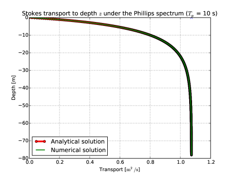
Figure 1: The Stokes transport between the surface and level $z$ under a Phillips spectrum (peak period 10 s). The analytical solution (9) is compared to a numerical integral and found to be identical to the numerical integration within numerical accuracy.

Appendix A The transport under a Phillips-type spectrum

The Stokes transport under Eq (7) can be written [following Eq (9)]

$$V(y_{0})=\frac{v_{0}}{2\overline{k}}\int_{y_{0}}^{0}\!\mathrm{e}^{-y}\,\mathrm{d}y-\beta\sqrt{\pi}\underbrace{\int_{y_{0}}^{0}\sqrt{y}\,\mathrm{erfc}\left(\sqrt{y}\right)}_{I_{1}}\,\mathrm{d}y.$$ (21)

Here we have introduced the variable substitution $y=-2\overline{k}z$. The integral $I_{1}$ can be solved by first substituting $u=\sqrt{y}$,

$$I_{1}=2\int_{0}^{u_{0}}u^{2}\,\mathrm{erfc}\,u\,\mathrm{d}u.$$ (22)

Integrate by parts to get

$$I_{1}=\frac{2}{3}u_{0}^{3}\,\mathrm{erfc}\,u_{0}+\frac{4}{3\sqrt{\pi}}\underbrace{\int_{0}^{u_{0}}u^{3}\mathrm{e}^{-u^{2}}\,\mathrm{d}u}_{I_{2}}.$$ (23)

The integral $I_{2}$ can be found analytically [see Eq (3.321.6) of Gradshteyn and Ryzhik 2007],

$$I_{2}=1-(1+u_{1}^{2})\mathrm{e}^{-u_{1}^{2}}.$$ (24)

Eq (21) can now be solved,

$$V(y_{0})=\frac{v_{0}}{2\overline{k}}\left\{1-\mathrm{e}^{-y_{0}}-\frac{2\beta}{3}\left[1+\sqrt{\pi}y_{0}^{3/2}\,\mathrm{erfc}\,\sqrt{y_{0}}-(1+y_{0})\mathrm{e}^{-y_{0}}\right]\right\}.$$ (25)

References

- Ardhuin et al. (2009) Ardhuin, F., Marié, L., Rascle, N., Forget, P., Roland, A., 2009. Observation and estimation of Lagrangian, Stokes and Eulerian currents induced by wind and waves at the sea surface. J Phys Oceanogr 39, 2820–2838. doi:10.1175/2009JPO4169.1.
- Breivik et al. (2013) Breivik, Ø., Allen, A., Maisondieu, C., Olagnon, M., 2013. Advances in Search and Rescue at Sea. Ocean Dyn 63, 83–88, arXiv:1211.0805. doi:10/jtx.
- Breivik et al. (2012a) Breivik, Ø., Allen, A., Maisondieu, C., Roth, J.C., Forest, B., 2012a. The Leeway of Shipping Containers at Different Immersion Levels. Ocean Dyn 62, 741–752, arXiv:1201.0603. doi:10.1007/s10236-012-0522-z. sAR special issue.
- Breivik and Allen (2008) Breivik, Ø., Allen, A.A., 2008. An operational search and rescue model for the Norwegian Sea and the North Sea. J Marine Syst 69, 99–113, arXiv:1111.1102. doi:10.1016/j.jmarsys.2007.02.010.
- Breivik et al. (2011) Breivik, Ø., Allen, A.A., Maisondieu, C., Roth, J.C., 2011. Wind-induced drift of objects at sea: The leeway field method. Appl Ocean Res 33, 100–109, arXiv:1111.0750. doi:10.1016/j.apor.2011.01.005.
- Breivik et al. (2012b) Breivik, Ø., Bekkvik, T.C., Ommundsen, A., Wettre, C., 2012b. BAKTRAK: Backtracking drifting objects using an iterative algorithm with a forward trajectory model. Ocean Dyn 62, 239–252, arXiv:1111.0756. doi:10.1007/s10236-011-0496-2.
- Breivik et al. (2016) Breivik, Ø., Bidlot, J.R., Janssen, P.A., 2016. A Stokes drift approximation based on the Phillips spectrum. Ocean Model 100, 49–56, arXiv:1601.08092. doi:10.1016/j.ocemod.2016.01.005.
- Breivik et al. (2014) Breivik, Ø., Janssen, P., Bidlot, J., 2014. Approximate Stokes Drift Profiles in Deep Water. J Phys Oceanogr 44, 2433–2445, arXiv:1406.5039. doi:10.1175/JPO-D-14-0020.1.
- Dee et al. (2011) Dee, D., Uppala, S., Simmons, A., Berrisford, P., Poli, P., Kobayashi, S., Andrae, U., Balmaseda, M., Balsamo, G., Bauer, P., P, B., Beljaars, A., van de Berg, L., Bidlot, J., Bormann, N., et al., 2011. The ERA-Interim reanalysis: Configuration and performance of the data assimilation system. Q J R Meteorol Soc 137, 553–597. doi:10.1002/qj.828.
- Gradshteyn and Ryzhik (2007) Gradshteyn, I., Ryzhik, I., 2007. Table of Integrals, Series, and Products, 7th edition. Edited by A. Jeffrey and D. Zwillinger, Academic Press, London.
- Kenyon (1969) Kenyon, K.E., 1969. Stokes Drift for Random Gravity Waves. J Geophys Res 74, 6991–6994. doi:10.1029/JC074i028p06991.
- Li et al. (2015) Li, Q., Webb, A., Fox-Kemper, B., Craig, A., Danabasoglu, G., Large, W.G., Vertenstein, M., 2015. Langmuir mixing effects on global climate: WAVEWATCH III in CESM. Ocean Model doi:10.1016/j.ocemod.2015.07.020.
- McWilliams et al. (1997) McWilliams, J., Sullivan, P., Moeng, C.H., 1997. Langmuir turbulence in the ocean. J Fluid Mech 334, 1–30. doi:10.1017/S0022112096004375.
- McWilliams et al. (2014) McWilliams, J.C., Huckle, E., Liang, J., Sullivan, P., 2014. Langmuir turbulence in swell. J Phys Oceanogr 44, 870–890. doi:10.1175/JPO-D-13-0122.1.
- McWilliams and Sullivan (2000) McWilliams, J.C., Sullivan, P.P., 2000. Vertical mixing by Langmuir circulations. Spill Science and Technology Bulletin 6, 225–237. doi:10.1016/S1353-2561(01)00041-X.
- Phillips (1958) Phillips, O.M., 1958. The equilibrium range in the spectrum of wind-generated waves. J Fluid Mech 4, 426–434. doi:10.1017/S0022112058000550.
- Reistad et al. (2011) Reistad, M., Breivik, Ø., Haakenstad, H., Aarnes, O.J., Furevik, B.R., Bidlot, J.R., 2011. A high-resolution hindcast of wind and waves for the North Sea, the Norwegian Sea, and the Barents Sea. J Geophys Res Oceans 116, 18 pp, C05019, arXiv:1111.0770. doi:10/fmnr2m.
- Roekel et al. (2012) Roekel, V., P., L., Fox-Kemper, B., Sullivan, P.P., Hamlington, P.E., Haney, S.R., 2012. The form and orientation of Langmuir cells for misaligned winds and waves. J Geophys Res Oceans 117, 22, C05001. doi:doi:10.1029/2011JC007516.
- Semedo et al. (2015) Semedo, A., Vettor, R., Breivik, Ø., Sterl, A., Reistad, M., Soares, C.G., Lima, D.C.A., 2015. The Wind Sea and Swell Waves Climate in the Nordic Seas. Ocean Dyn 65, 223–240. doi:10.1007/s10236-014-0788-4. 13th wave special issue.
- Webb and Fox-Kemper (2015) Webb, A., Fox-Kemper, B., 2015. Impacts of wave spreading and multidirectional waves on estimating Stokes drift. Ocean Model 96, 49–64. doi:10.1016/j.ocemod.2014.12.007.