Gaussian Process Morphable Models

Abstract

Models of shape variations have become a central component for the automated analysis of images. Statistical shape models (SSMs) represent a class of shapes as a normal distribution of point variations, whose parameters are estimated from example shapes. Principal component analysis (PCA) is applied to obtain a low-dimensional representation of the shape variation in terms of the leading principal components. In this paper, we propose a generalization of SSMs, which we refer to as Gaussian Process Morphable Models (GPMMs). We model the shape variations with a Gaussian process, which we represent using the leading components of its Karhunen-Loève expansion. To compute the expansion, we make use of an approximation scheme based on the Nyström method. The resulting model can be seen as a continuous analogon of a standard SSM. However, while for SSMs the shape variation is restricted to the linear span of the example data, with GPMMs we can define the shape variation using any Gaussian process. For example, we can build shape models that correspond to classical spline models, and thus do not require any example data. Furthermore, Gaussian processes make it possible to combine different models. For example, an SSM can be extended with a spline model, to obtain a model that incorporates learned shape characteristics, but is flexible enough to explain shapes that cannot be represented by the SSM.

We introduce a simple algorithm for fitting a GPMM to a surface or image. This results in a non-rigid registration approach, whose regularization properties are defined by a GPMM. We show how we can obtain different registration schemes, including methods for multi-scale, spatially-varying or hybrid registration, by constructing an appropriate GPMM. As our approach strictly separates modelling from the fitting process, this is all achieved without changes to the fitting algorithm.

We show the applicability and versatility of GPMMs on a clinical use case, where the goal is the model-based segmentation of 3D forearm images. In a first experiment we show how we can build GPMMs that are specially tailored to the task of forearm registration. We demonstrate how GPMMs can be used to advance standard Active Shape Models based segmentation. Finally, we show the application of GPMMs for the problem of 3D image to image registration. To complement the paper, we have made all our methods available as open source.

1 Introduction

The automatic interpretation and analysis of objects in an image is the core of computer vision and medical image analysis. A popular approach is analysis by synthesis [1], which asserts that in order to explain an image, we need to be able to synthesize its content. This is achieved by fitting a probabilistic model to an image, such that one-to-one correspondence between the model and the image is achieved. The image can then be explained using the model information. The better the model represents the structure of the objects to be analyzed, the easier it becomes to fit the model. For this reason statistical shape models have become very popular. The most important examples of statistical shape models are the Active Shape Model [2] and the Morphable model [3], which learn the shape variation from given training examples, and represent the shape variation using the leading principal components. In the following, we refer to this type of model as PCA-based statistical shape models, or in short SSMs. These models are linear, parametric models and hence are mathematically convenient and easy to incorporate in image-analysis algorithms. Since they can represent only shapes that are in the linear span of the given training examples, they lead to algorithms that are robust towards artifacts and noise. The downside of this specificity is that to learn a model that can express all possible target shapes, a lot of training data is needed.

The main contribution of this work is that we introduce a generalization of SSMs, which we refer to as Gaussian Process Morphable Models (GPMM). We model a shape as a deformation $u$ from a reference shape $\Gamma_{R}\subset\mathbb{R}^{3}$, i.e. a shape $s$ can be represented as

$$s=\{x+u(x)|x\in\Gamma_{R}\}$$

for some deformation $u:\Omega\to\mathbb{R}^{3}$, with $\Omega\supseteq\Gamma_{R}$. We model the deformation as a Gaussian process $u\sim GP(\mu,k)$ where $\mu:\Omega\to\mathbb{R}^{3}$ is a mean deformation and $k:\Omega\times\Omega\to\mathbb{R}^{3\times 3}$ a covariance function or kernel. The core idea behind our approach is that we obtain a parametric, low-dimensional model by representing the Gaussian process using the $r$ leading basis function $\phi_{i}:\Omega\to\mathbb{R}^{3}$ of its Karhunen-Loève expansion:

$$u=\mu+\sum_{i=1}^{r}\alpha_{i}\sqrt{\lambda_{i}}\phi_{i},\;\alpha_{i}\in\mathcal{N}(0,1)$$ (1)

(here, $\lambda_{i}$ is the variance associated with each basis function $\phi_{i}$). As we usually assume strong smoothness of the deformation when modelling shapes, it is often possible to achieve good approximations using only a few leading eigenvalues, which makes the representation practical. The main difficulty of this approach is to efficiently compute the leading eigenfunction/eigenvalue pairs. To this end, we propose to use a Nyström approximation, and make use of a recently introduced computational approach, which is able to use a large number of input points for computing the approximation [4]. We study the approximation properties of the numerical method and provide a detailed discussion of how the approximation quality is influenced by different chooses of covariance functions. Furthermore, we discuss how to chose the parameters of our method in order to reach a given approximation quality.

The biggest advantage of GPMMs compared to SSMs is that we have much more freedom in defining the covariance function. As a second main contribution we will show in Section 3 how expressive prior models for registration can be derived, by leveraging the modeling power of Gaussian processes. By estimating the covariances from example data our method becomes a continuous version of an SSM. When we have no or only little training data available, arbitrary kernel functions can be used to define the covariances. In particular we can define models of smooth deformations using spline models or radial basis functions, which are frequently used in registration approaches. We show how a simple registration approach, whose regularization properties are defined in terms of a GPMM, allows us to use these models for actual surface and image registration. Besides these simple models, GPMMs also make it possible to combine different covariance functions (or kernels) to mimic more sophisticated registration schemes. We show how to construct priors that have multi-scale properties, are spatially-varying or incorporate landmark constraints. We will also show how to combine models learned from training data with analytically defined covariance functions, in order to increase the flexibility of SSMs in cases where not sufficient training data is available. Although in contrast to SSMs, GPMMs model deformations defined on a continuous domain, we can always discretize it to obtain a model that is mathematically equivalent to an SSM. This makes it possible to leverage the modelling flexibility of GPMMs also in classical shape modelling algorithms, such as for example the Active Shape Model fitting [2] algorithm or the coherent point drift method [5].

We have implemented our method for modeling with Gaussian processes as part of the open source software statismo [6] and scalismo [7]. We perform registration experiments on a real world data-set of forearm images with associated ground-truth segmentations. In a first experiment we show how GPMMs can be specially tailored to the task of forearm registration, and perform surface-to-surface registration experiments with different models. In the second experiment we show how Active Shape Model fitting can be improved by using GPMMs as a shape prior. In the last experiment, we present an application of GPMMs for 3D image-to-image registration and compare the result to the popular B-spline registration method implemented in Elastix [49].

1.1 Related work

Our work can be seen as the unification of two different concepts: On one hand we extend SSMs, such that they become more expressive, on the other hand we model prior distributions for surface and image registration. There are works from both the shape modelling and the registration community, which are conceptually similar or have the same goals as we pursuit with our approach. Most notably, the work of Wang and Staib [8], which aims for extending the flexibility of shape models, and the work by Grenander et al. [9], who use Gaussian processes as priors for registration are very close in spirit to our model. The idea of Wang and Staib is to extend the flexibility of a SSM by combining a learned covariance matrix used in a statistical shape model with covariance matrices that represent other, synthetic deformations. This corresponds exactly to our idea for combining covariance functions in the GP setting. However, their method requires that the full covariance matrix can be represented, which is only feasible for very coarsely discretized shapes. In contrast, our method yields a continuous representation, and allows for an arbitrarily fine discretization once the prior is evaluated in the final registration procedure. On the registration side, the use of Gaussian processes for image registration has been extensively studied in the 90s by Grenander et al. (see the overview article [9] and references therein). Similar to our approach, they propose to use a basis function representation to span the model space. However, in all these works the basis functions have to be known analytically [10], or the initial model needs to be of finite rank [11]. In our method we use of the Nyström approximation to numerically approximate the leading eigenfunctions, which makes it possible to approximate any Gaussian process and thus to allow us to use arbitrary combinations of kernels in our models. We believe that this modelling flexibility is what makes this approach so powerful.

There are many other works that propose to model the admissible deformations for non-rigid registration by means of a kernel (i.e. as a Reproducing Kernel Hilbert Space (RKHS)). Especially for landmark based registration, spline based models and radial basis functions have been widely used [12]. The algorithm for solving a standard spline-based landmark registration problem corresponds to the MAP solution in Gaussian process regression [13]. Using Gaussian process regression directly for image registration has been proposed by Zhu et al [14]. A similar framework for surface registration, where kernels are used for specifying the admissible deformation was proposed by Steinke et al. [15]. While they do not provide a probabilistic interpretation of the problem, their approach results in the same final registration formulation as our approach. The use of Reproducing Kernel Hilbert Spaces for modeling admissible deformation also plays an important role for diffeomorphic image registration (see e.g. [16], Chapter 9). In this context, it has also been proposed to combine basic kernels for multi-scale [17, 18] and spatially-varying models [19] for registration. However, the work focuses more on the mathematical and algorithmic aspects of enforcing diffeomorphic mappings, rather than modelling aspect.

Besides the work of Wang and Staib [8] there have been many other works for extending the flexibility of SSMs. This is typically achieved by adding artificial training data [20] or by segmenting the model either spatially [21, 3] or in the frequency domain [22, 23]. The use of Gaussian processes to model the covariance structure is much more general and subsumes all these methods. Another set of work gives shape model based algorithms more flexibility for explaining a target solution [24, 25, 26]. Compared to our model, these approaches have the disadvantage that the model is not generative anymore and does not admit a clear probabilistic interpretation.

This paper is a summary and extension of our previous conference publications [27, 28, 29]. It extends our previous work in several ways: 1) It provides an improved presentation of the basic method and in particular its numeric implementation. 2) It provides an analysis of the approximation properties of this scheme. 3) It proposes new combination of kernels to combine statistical shape models and analytically defined kernels. 4) It features a more detailed validation including surface and image registration, as well as Active Shape Model fitting.

2 Gaussian Process Morphable Models

Before describing GPMMs, we summarize the main concepts of PCA-based statistical shape models, on which we will build up our work.

2.1 PCA-based statistical Shape models

PCA-based statistical shape models assume that the space of all possible shape deformation can be learned from a set of typical example shapes $\{\Gamma_{1},\ldots,\Gamma_{n}\}$. Each shape $\Gamma_{i}$ is represented as a discrete set of landmark points, i.e.

$$\Gamma_{i}=\{x_{k}^{i}\,|\,x_{k}\in\mathbb{R}^{3},k=1,\ldots,N\},$$

where $N$ denotes the number of landmark points. In early approaches, the points typically denoted anatomical landmarks, and $N$ was consequently small (in the tens). Most modern approaches use a dense set of points to represent the shapes. In this case, the number of points is typically in the thousands. The crucial assumption is that the points are in correspondence among the examples. This means that the $k$-th landmark point $x_{k}^{i}$ and $x_{k}^{j}$ of two shapes $\Gamma_{i}$ and $\Gamma_{j}$ represent the same anatomical point of the shape. These corresponding points are either defined manually, or automatically determined using a registration algorithm. To build the model a shape $\Gamma_{i}$ is represented as a vector $s_{i}\in\mathbb{R}^{3N}$, where the $x,y,z-$ components of each point are stacked onto each other:

$$\vec{s_{i}}=(x_{1x}^{i},x_{1y}^{i},x_{1z}^{i},\ldots,x_{Nx}^{i},x_{Ny}^{i},x_{Nz}^{i}).$$

This vectorial representation makes it possible to apply the standard multivariate statistics to model a probability distribution over shapes. The usual assumption is that the shape variations can be modelled using a normal distribution

$$s\sim\mathcal{N}(\mu,\Sigma)$$

where the mean $\mu$ and covariance matrix $\Sigma$ are estimated from the example data:

$$\mu =\overline{s}:=\frac{1}{n}\sum_{i=1}^{n}\vec{s}_{i}$$ (2)

$$\Sigma =S:=\frac{1}{n-1}\sum_{i=1}^{n}(\vec{s}_{i}-\overline{s})(\vec{s}_{i}-\overline{s})^{T}.$$ (3)

As the number of points $N$ is usually large, the covariance matrix $\Sigma$ cannot be represented explicitly. Fortunately, as it is determined completely by the $n$ example data-sets, it has at most rank $n$ and can therefore be represented using $n$ basis vectors. This is achieved by performing a Principal Component Analysis (PCA) [30]. In its probabilistic interpretation, PCA leads to a model of the form

$$s=\overline{s}+\sum_{i=1}^{n}\alpha_{i}\sqrt{d_{i}}\vec{u}_{i}$$ (4)

where $(u_{i},d_{i}),\,i=1,\ldots,n$, are the eigenvectors and eigenvalues of the covariance matrix $S$. Assuming that $\alpha_{i}\sim\mathcal{N}(0,1)$ in (4), it is easy to check that $s\sim\mathcal{N}(\overline{s},S)$. Thus, we have a efficient, parametric representation of the distribution.

2.2 Gaussian Process Morphable Models

The literature of PCA based statistical shape models usually emphasizes the shapes that are modelled. Equation 4 however, gives rise to different interpretation: A statistical shape model is a model of deformations $\vec{\phi}=\sum_{i=1}^{n}\alpha_{i}\sqrt{d_{i}}\vec{u}_{i}\sim\mathcal{N}(0,S)$ which are added to a mean shape $\overline{s}$. The probability distribution is on the deformations. This is the interpretation we use when we generalize these models to define Gaussian Process Morphable Models. We define a probabilistic model directly on the deformations. To stress that we are modelling deformations (i.e. vector fields defined on the reference domain $\Gamma_{R}$), and to become independent of the discretization, we model the deformations as a Gaussian process.

Let $\Gamma_{R}\subset\mathbb{R}^{3}$ be a reference shape and denote by $\Omega\subset\mathbb{R}^{3}$ a domain, such that $\Gamma_{R}\subseteq\Omega$. We define a Gaussian process $u\in\mathcal{GP}(\mu,k)$ with mean function $\mu:\Omega\to\mathbb{R}^{3}$ and covariance function $k:\Omega\times\Omega\to\mathbb{R}^{3\times 3}$. Note that any deformation $\hat{u}$ sampled from $\mathcal{GP}(\mu,k)$, gives rise to a new shape by warping the reference shape $\Gamma_{R}$:

$$\Gamma=\{x+\hat{u}(x)\,|\,x\in\Gamma_{R}\}.$$

Similar to the PCA representation of a statistical shape model used in (Equation 4), a Gaussian process $\mathcal{GP}(\mu,k)$ can be represented in terms of an orthogonal set of basis functions $\{\phi_{i}\}_{i=1}^{\infty}$

$$u(x)\sim\mu(x)+\sum_{i=1}^{\infty}\alpha_{i}\sqrt{\lambda}_{i}\phi_{i}(x),\,\alpha_{i}\in\mathcal{N}(0,1),$$ (5)

where $(\lambda_{i},\phi_{i})$ are the eigenvalue/eigenfunction pairs of the integral operator

$$\mathcal{T}_{k}f(\cdot):=\int_{\Omega}k(x,\cdot)f(x)\,d\rho(x),$$

where $\rho(x)$ denotes a measure. The representation (5) is known as the Karhunen-Loève expansion of the Gaussian process [31]. Since the random coefficients $\alpha_{i}$ are uncorrelated, the variance of $u$ is given by the sum of the variances of the individual components. Consequently, the eigenvalue $\lambda_{i}$ corresponds to the variance explained by the $i$-th component. This suggests that if the $\lambda_{i}$ decay sufficiently quickly, we can use the low-rank approximation

$$\tilde{u}(x)\sim\mu(x)+\sum_{i=1}^{r}\alpha_{i}\sqrt{\lambda}_{i}\phi_{i}(x)$$ (6)

to represent the process. The expected error of this approximation is given by the tail sum

$$\sum_{i=r+1}^{\infty}\lambda_{i}.$$

The resulting model is a finite dimensional, parametric model, similar to a standard statistical model. Note, however, that there is no restriction that the covariance function $k$ needs to be the sample covariance matrix. Any valid positive definite covariance function can be used. As we will show in Section 3 this makes it possible to define powerful prior models, even when there is little or no example data available.

2.3 Computing the eigenfunctions

The low-rank approximation (6) can only be performed if we are able to compute the eigenfunction/eigenvalue pairs $(\phi_{i},\lambda_{i})_{i=1}^{r}$. Although for some kernel functions analytic solutions are available (see e.g. [10, 9]) for most interesting models we need to resort to numeric approximations. A classical method, which has recently received renewed attention from the machine learning community, is the Nyström method [13]. The goal of the Nyström method is to obtain a numerical estimate for the eigenfunctions/eigenvalues of the integral operator

$$\mathcal{T}_{k}f(\cdot):=\int_{\Omega}k(x,\cdot)f(x)d\rho(x).$$ (7)

The pairs $(\phi_{i},\lambda_{i})$, satisfying the equation

$$\lambda_{i}\phi_{i}(x^{\prime})=\int_{\Omega}k(x,x^{\prime})\phi_{i}(x)\,d\rho(x),\;\forall x^{\prime}\in\Omega$$ (8)

are sought. The Nyström method is intended to approximate the integral in (8). This can, for example, be achieved by letting $d\rho(x)=p(x)\,dx$ where $p(x)$ is a density function defined on the domain $\Omega$, and to randomly sample points $X=\{x_{1},\ldots,x_{n}\},x_{l}$ according to $p$. The samples $(x_{l})_{l=1,\ldots,N}$ for $x^{\prime}$ in (8) lead to the matrix eigenvalue problem

$$Ku_{i}=\lambda_{i}^{mat}u_{i},$$ (9)

where $K_{il}=k(x_{i},x_{l})$ is the kernel matrix, $u_{i}$ denotes the $i-$th eigenvector and $\lambda_{i}^{mat}$ the corresponding eigenvalue. Note, that since the kernel is matrix valued ($k:\Omega\times\Omega\to\mathbb{R}^{d\times d}$), the matrices $K$ and $k_{X}$ are block matrices: $K\in\mathbb{R}^{nd\times nd}$ and $k_{X}\in\mathbb{R}^{nd\times d}$. The eigenvalue $\lambda_{i}^{mat}$ approximates $\lambda_{i}$, while the eigenfunction $\phi_{i}$ in turn is approximated with

$$\tilde{\phi}_{i}(x)=\frac{\sqrt{n}}{\lambda_{i}^{mat}}k_{X}(x)u_{i}\approx\phi_{i}(x),$$ (10)

where $k_{X}(x)=(k(x_{1},x),\ldots,k(x_{n},x))$.

Clearly, the quality of this approximation improves with the number of points $n$, which are sampled (see Appendix A for a detailed discussion). As $n$ becomes larger (i.e. exceeds a few thousand points), deriving the eigenvalue problem (9) might still be computationally infeasible. Following Li et al. [4], we therefore apply a random SVD [32] for efficiently approximating the first eigenvalues/eigenvectors without having to compute the eigenvalues of the full $N\times N$ matrix. Theoretical bounds of the method [32], as well as its application for the Nyström approximation [4] show that it leads to accurate approximation for kernels with a fast decaying spectrum. For our application, the error induced by the random SVD is negligible compared to the approximation error caused by the low-rank approximation and the Nyström method.

2.4 Accuracy of the low-rank approximation

It is clear that our method depends crucially on the quality of the low-rank approximations. Ideally, we would like to see the low-rank model as a convenient reparametrization of the original process, which would not affect the shape variations that are spanned by our model. Unfortunately, and not surprisingly, this is not always the case. There are two sources of error: 1) There is no good representation of the Gaussian process in terms of the leading basis-functions 2) Even if there is, it might still happen that the numerical computation of the eigenvalues using the Nyström method leads to approximation errors. In order not to digress from the main theme of the paper, we have put a detailed discussion of these issues into the appendix (cf. Appendix A), and summarize here only the main results.

Intuitively, the ability to represent a model using only a few leading basis functions is dependent on how much the individual points of the models correlate. This becomes clear when we consider the two extreme cases: 1) All points are perfectly linearly correlated and 2) every point can move independently. We can simulate these extreme using a Gaussian kernel $k(x,x^{\prime})=\exp(-\frac{\lVert x-x^{\prime}\rVert^{2}}{\sigma^{2}})$, where we choose $\sigma^{2}\to\infty$ to simulate the first case. In this case all points are perfectly correlated and the process can be represented using a single basis function. The second extreme case is attained if we let $\sigma^{2}$ approach $0$ (i.e. the kernel becomes the $\delta$-function $\delta_{xx^{\prime}}$). In this case, any point can move independently, and to faithfully represent the process, we need one basis function per point. From these considerations we can see that the larger the assumed smoothness of the process (and hence the correlation between the points), the fewer basis functions are needed to approximate the process. It is also intuitively clear that the Nyström approximation yields much better results in the first case. As there are strong correlations between the points, the knowledge of the true eigenfunction value at the Nyström points $x_{1},\ldots,x_{n}$ will also determine the value of the basis function at the correlated points. This is no longer the case where we don’t have correlations. In this case, knowing the value at the points $x_{1},\ldots,x_{n}$ will not give us any information about the value of the basis function at other points of the domain.

3 Modeling with kernels

The formalism of Gaussian processes provides us with a rich language to model shape variations. In this section we explore some of these modelling possibilities, with a focus on models that we find most useful in our work on model-based image analysis and in particular surface and image registration. Many more possibilities for modelling with Gaussian processes have been explored in the machine learning community (see e.g. Duvenaud, Chapter 2 [33]).

To visualize the shape variations represented by a model, we define a GPMM on the face surface (see Figure 1) and show the effect that randomly sampled deformation from this model have on this face surface. Using the face for visualizing shape variations has the advantage that we can judge how anatomically valid a given shape deformation is.

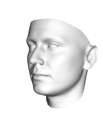
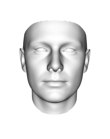
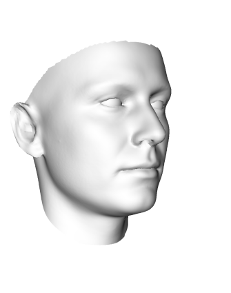
Figure 1: The 3D face surface used to illustrate the effect of different models.

3.1 Models of smooth deformations

A simple Gaussian process model is a zero mean Gaussian process that enforces smooth deformations. The assumption of a zero mean is typically made in registration tasks. It implies that the reference surface is a representative shape for the class of shapes which are modelled, that is the shape is close to a (hypothetical) mean shape. A particularly simple kernel that enforces smoothness is the Gaussian kernel defined by

$$k_{g}(x,y)=\exp(-\lVert x-y\rVert^{2}/\sigma^{2}),$$

where $\sigma^{2}$ defines the range over which deformations are correlated. Hence the larger the values of $\sigma$, the more smoothly varying the resulting deformations fields will be. In order to use this scalar-valued kernel for registration, we define the matrix valued kernel

$$k(x,y)=s\cdot I_{3\times 3}k_{g}(x,y),$$

where the identity matrix $I_{3\times 3}$ signifies that the $x,y,z$ component of the modelled vector field are independent. The parameter $s\in\mathbb{R}$ determines the variance (i.e. scale) of a deformation vector. Figure 2 shows random samples from the model for two different values of $\sigma$.

Besides Gaussian kernels, there are many different kernels that are known to lead to smooth functions. For registration purposes, spline models, Elastic-Body Splines [35] B-Splines [36] or Thin Plate Splines [37] are maybe the most commonly used. Another useful class of kernels that enforce smoothness is given by the Matérn class of kernels (see e.g. [13], Chapter 4), which allows us to explicitly specify the degree of differentiabiliy of the model.

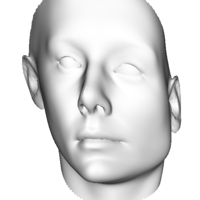
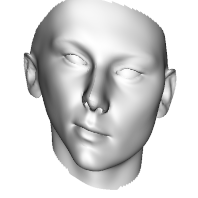
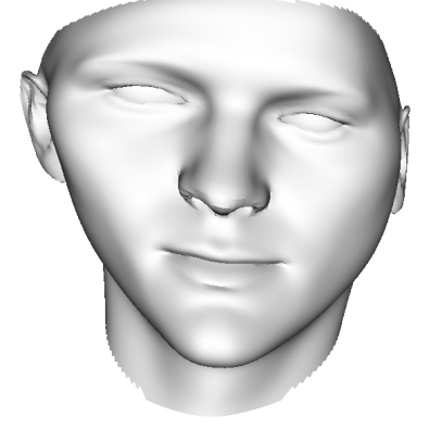
(a) $s=100,\sigma=100$ mm

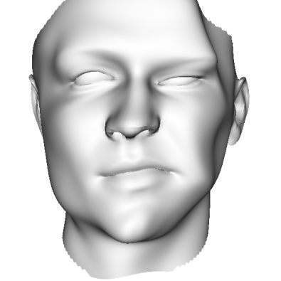
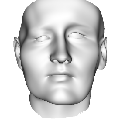
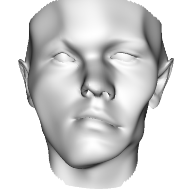
(b) $s=10,\sigma=30$ mm

Figure 2: Samples using a Gaussian kernel with scale factor $s$ and bandwidth $\sigma$. Choose $\sigma$ large leads to smooth, global deformations of the face, while choosing it small yields more local deformations.

3.2 Statistical shape models

The smoothness kernels are generic, in the sense that they do not incorporate prior knowledge about a shape. This is reflected in Figure 2, where the sampled faces do not look like valid anatomical face shapes. An ideal prior for the registration of faces would only allow valid face shapes. This is the motivation behind SSMs [2, 3]. The characteristic deformations are learned from a set of typical examples surfaces $\Gamma_{1},\ldots,\Gamma_{n}$. More precisely, by establishing correspondence, between a reference $\Gamma_{R}$ and each of the training surfaces, we obtain a set of deformation fields $\{u_{1},\ldots,u_{n}\},u_{i}:\Omega\to\mathbb{R}^{d}$, where $u_{i}(x)$ denotes a deformation field that maps a point on the reference $x\in\Gamma_{R}$ to its corresponding point $u_{i}(x)$ on the $i-$th training surface. A Gaussian process $\mathcal{GP}(\mu_{SM},k_{SM})$ that models these characteristic deformations is obtained by estimating the empirical mean

$$\mu_{SM}(x)=\frac{1}{n}\sum_{i=1}^{n}u_{i}(x)$$

and covariance function

$$k_{SM}(x,y)=\frac{1}{n-1}\sum_{i=1}^{n}(u_{i}(x)-\mu_{SM}(x))(u_{i}(y)-\mu_{SM}(y))^{T}.$$ (11)

We refer to the kernel $k_{SM}$ as the sample covariance kernel or empirical kernel. Samples from such a model are depicted in Figure 3, where the variation was estimated from 200 face surfaces from the Basel Face Model [34]. In contrast to the smoothness priors, all the sampled face surfaces represent anatomically plausible faces. The model that we obtain using this sample covariance kernel is a continuous analogon to a PCA based shape model.

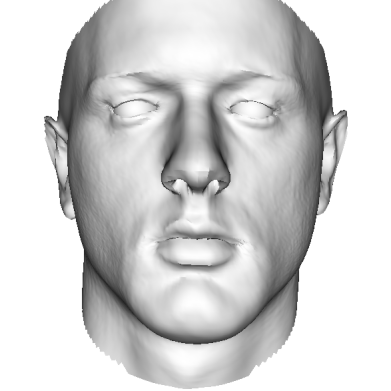
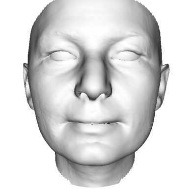
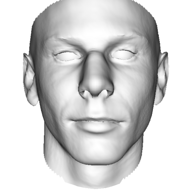
Figure 3: Samples using a sample covariance kernel, which is learned from 200 training faces. All the random samples look like valid faces.

3.3 Combining kernels

The kernels that we have discussed so far already provide a large variety of different choices for modeling prior assumptions. But the real power of these models comes to bear if the “simple“ kernels are combined to define new kernels, making use of a relative rich algebra that kernels admit. In the following, we present basic combinations of kernels to give the reader a taste of what can be achieved. For a more thorough discussion of how positive definite kernels can be combined, we refer the reader to Shawe-Taylor et al. [38] (Chapter 3, Proposition 3.22).

3.3.1 Multiscale models

If $k_{1},\ldots,k_{n}:\Omega\times\Omega\to\mathbb{R}^{d\times d}$ are positive definite kernels, then the linear combination

$$k_{S}(x,x^{\prime})=\sum_{i=1}^{l}\alpha_{i}k_{i}(x,x^{\prime}),\;\alpha_{i}\in\mathbb{R}$$

is positive definite as well. This provides a simple means of modeling deformations on multiple scale levels by summing kernels that model smooth deformations with kernels for more local, detailed deformation. A particularly simple implementation of such a strategy is to sum up Gaussian kernels, with decreasing scale and bandwidth:

$$k_{MS}(x,x^{\prime})=\sum_{i=1}^{l}\frac{s}{i}I_{3\times 3}\exp(-\frac{\lVert x-x^{\prime}\rVert^{2}}{(\sigma/i)^{2}})$$

where $s$ determines the base scale and $\sigma$ the smoothness and $l$ the number of levels. As shown in Figure 4, this simple approach already leads to a multiscale structure that models both large scale deformations as well as local details. This idea could be extended to obtain wavelet-like multi-resolution strategies, by choosing the kernels to be refinable (which is, for example true for the B-spline kernel). A more detailed discussion of such kernels is given in [39, 40].

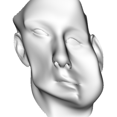
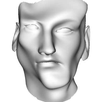
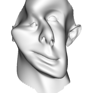
Figure 4: Samples using a kernel defined on multiple scales. The random sample show large deformations which change the overall face shape, as well as local, detailed shape variations.

3.3.2 Reducing the bias in statistical shape models

Another use case that makes use of the possibility to add two kernels is to explicitly model the bias of a statistical shape model. Due to the limited availability of training examples, statistical shape models are often not able to represent the full shape space accurately and thus introduce a bias towards the training shapes into model-based methods [26]. One possibility to avoid this problem is to provide an explicit bias model. Denote by $k_{SM}:\Omega\times\Omega\to\mathbb{R}^{d\times d}$ the sample covariance kernel and let $k_{g}:\Omega\times\Omega\to\mathbb{R}$ be a Gaussian kernel with bandwidth parameter $\sigma$. A simple model to reduce the bias would be to use a Gaussian kernel with a large bandwidth, i.e. we define

$$k_{b}(x,x^{\prime})=k_{SM}(x,x^{\prime})+sI_{3\times 3}k_{g}(x,x^{\prime}),$$

where the parameter $s$ defines the scale of the average error. This parameter could, for example, be estimated using crossvalidation. This simple model assumes that the error is spatially correlated, i.e. if a model cannot explain the structure at a certain point, its neighboring points are likely to also show the same error. An example of how this strategy can reduce the bias in statistical shape models is given in our previous publication [29].

3.3.3 Localizing models

Another possibility to obtain more flexible models is to make models more local. Recalling that the kernel function $k(x,x^{\prime})$ models the correlation between point $x$ and $x^{\prime}$, we see that setting the correlation $k(x,x^{\prime})$ to $0$ for $x\neq x^{\prime}$ decouples the points and hence increases the flexibility of a model. Such an effect can be achieved by a multiplication of two kernel functions, which again results in a positive definite kernel. A simple example of a local model is obtained by multiplying a kernel with a Gaussian kernel. For example, by defining

$$k_{l}(x,x^{\prime})=k_{SM}(x,x^{\prime})\odot I_{3\times 3}k_{g}(x,x^{\prime})$$

(where $\odot$ defines element wise multiplication), we obtain a localized version of a statistical shape model. Samples from such a model are shown in Figure 5. We observe that the samples locally look like valid faces, but globally, the kernel still allows for more flexible variations, which could not be described by the model, and which may not constitute an anatomically valid face.

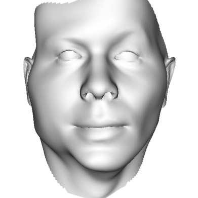
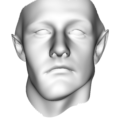
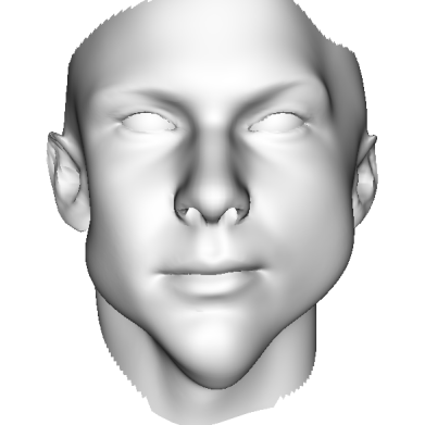
Figure 5: Random samples form a localized statistical shape model. Whereas locally the variations look anatomically valid, there are no global correlations anymore, which makes the model more flexible.

3.3.4 Spatially varying models

Taking these ideas one step further, we can also combine the two approaches and sum up several localized models to obtain a non-stationary kernel. The use of such kernels in the context of registration has recently been proposed by Schmah et al. [19], who showed how it can be used in a method for spatially-varying registration.

Let $\Omega=(\Omega_{1},\ldots,\Omega_{n})$ be a partition of the domain $\Omega$ into several regions $\Omega_{i}$ and associate to each region a kernel $k^{i}$ with the desired characteristics. We define a weight functions $w_{i}:\Omega\to[0,1]$, such that $\sum_{i}w_{i}(x)=1$. The weight function $w_{i}$ is chosen such that $w_{i}(x)=1$ for the region $\Omega_{i}$. For any real valued function $f$ the kernel $k(x,x^{\prime})=f(x)f(x^{\prime})$ is positive definite, and we can define a “localization“ kernel

$$k_{l}^{i}(x,x^{\prime})=w_{i}(x)w_{i}(x^{\prime}).$$

The final spatially-varying model $\mathcal{GP}(0,k_{sv})$ using this kernel is defined by

$$k_{sv}(x,x^{\prime})=\sum_{i}k_{l}^{i}(x,x^{\prime})k^{i}(x,x^{\prime}).$$

Figure 6 shows samples from a model where the upper part of the face is modelled using a statistical model, while the lower part (below the nose) undergoes arbitrary smooth deformations.

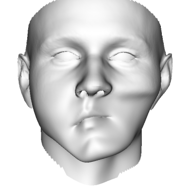
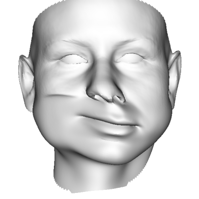
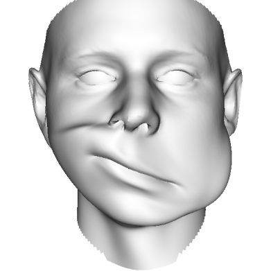
Figure 6: Random samples form a spatially-varying model. The variation in the upper part of the face is model using a sample covariance kernel while the lower part uses a Gaussian kernel.

3.4 Posterior models

Modeling by combining different kernels amounts to specifying our prior assumptions by modeling how points correlate. In many applications we have not only information about the correlations, but know for certain points exactly how they should be mapped. Assume for instance, that a user has clicked a number of landmark points on a reference shape ${L_{R}}=\{l_{R}^{1},\ldots,l_{R}^{n})\}$ together with the matching points on a target surface ${L_{T}}=\{l_{T}^{1},\ldots,l_{T}^{n})\}$. These landmarks provide us with known deformation at the matching points, i.e.

$${L}=\{(l_{R}^{1},l_{T}^{1}-l_{R}^{1}),\ldots,(l_{R}^{n},l_{T}^{n}-l_{R}^{n})\}=:\{(l_{R}^{1},\hat{u}^{1}),\ldots,(l_{R}^{n},\hat{u}^{n})\}.$$

Assuming further that the deformations $\hat{u}^{i}$ are subject to Gaussian noise $\epsilon\sim I_{3\times 3}\sigma$, we can use Gaussian process regression to compute from a given Gaussian process $GP(\mu,k)$ a new Gaussian process, known as the posterior process or posterior model, $\mathcal{GP}(\mu_{p},k_{p})$ (cf. [13], Chapter 2). Its mean $\mu_{p}$ and covariance $k_{p}$ are known in closed form and given by

$$\mu_{p}(x) =\mu(x)+K_{X}(x)^{T}(K_{XX}+\sigma^{2}\mathcal{I})^{-1}\hat{U}$$ (12)

$$k_{p}(x,x^{\prime}) =k(x,x^{\prime})-K_{X}(x)^{T}(K_{XX}+\sigma^{2}\mathcal{I})^{-1}K_{X}(x^{\prime}).$$ (13)

Here, we defined $K_{X}(x)=(k(x,x_{i}))_{i=1}^{n}\in\mathbb{R}^{3n\times 3}$, $K_{XX}=\left(k(x_{i},x_{j})\right)_{i,j=1}^{n}\in\mathbb{R}^{3n\times 3n}$ and $\hat{U}=(\hat{u}^{1}-\mu(x),\ldots,\hat{u}^{n}-\mu(x))^{T}\in\mathbb{R}^{3n}$. Note that $K_{X}$ and $K_{XX}$ consist of sub-matrices of size $3\times 3$. The posterior is again a Gaussian process, and hence is itself a (data-dependent) GPMM, which we can use anywhere we would use a standard GPMM. Figure 7 shows random samples from such prior, where the points shown in red are fixed by setting $(\hat{u}^{i}=(0,0,0)^{T}),i=1,\ldots,n)$.

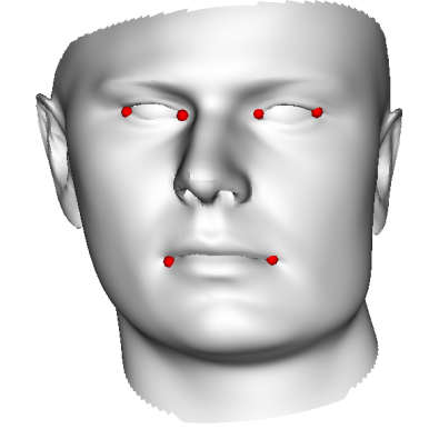
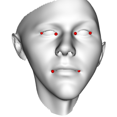
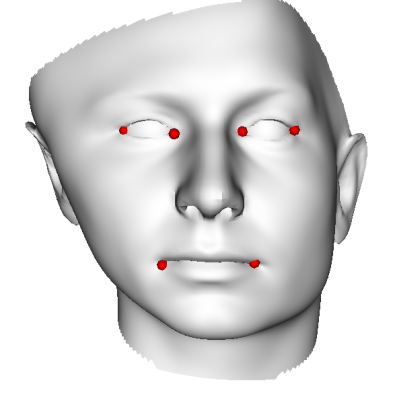
(a) $s=10,\sigma=30mm$

Figure 7: Random samples from a posterior model, which has been obtained by taking the Gaussian process model shown in Figure 2a, and applying Gaussian process regression to keep the points shown in red fixed.

4 Registration using Gaussian Process Morphable Models

In this section we show how we can use GPMMs as prior models for surface and image registration. The idea is that we define a model for the variability of a given object $O_{R}\subset\mathbb{R}^{d}$ and fit this model to a target image or surface $O_{T}\subset\mathbb{R}^{d}$. Our main assumption is that we can identify for each point $x_{R}\in O_{R}$, a corresponding point $x_{T}\in O_{T}$ of the target object $O_{T}$. More formally, it is assumed that there exists a deformation $u:\Omega\to\mathbb{R}^{d}$, such that

$$O_{T}=\{x+u(x)|x\in O_{R}\}.$$

The goal of the registration problem is to recover the deformation field $u$, that relate the two objects.

To this end, we formulate the problem as a MAP estimate:

$$\operatornamewithlimits{arg\,max}_{u}p(u)p(O_{T}|O_{R},u),$$ (14)

where $p(u)\sim\mathcal{GP}(\mu,k)$ is a Gaussian process prior over the admissible deformation fields and $p(O_{T}|O_{R},u)=\frac{1}{Z}\exp(\eta^{-1}\mathcal{D}[O_{R},O_{T},u])$, $\mathcal{D}$ is a metric that measures the similarity of the objects $O_{T},O_{R}$. Here $\eta\in\mathbb{R}$ is a weighting parameter and $Z$ a normalization constant. In order to find the MAP solution, we reformulate the registration problem as an energy minimization problem. It is well known (see e.g. [41] for details) that the solution to the MAP problem (14) is attainable by minimizing in the RKHS $\mathcal{F}_{k}$ defined by $k$ :

$$\operatornamewithlimits{arg\,min}_{u\in\mathcal{F}_{k}}\mathcal{D}[O_{R},O_{T},u]+\eta\lVert u\rVert_{k}^{2},$$ (15)

where $\lVert\cdot\rVert_{k}$ denotes the RKHS norm. Using the low-rank approximation (Equation (6)) we can restate the problem in the parametric form

$$\operatornamewithlimits{arg\,min}_{\alpha_{1},\ldots,\alpha_{r}}\mathcal{D}[O_{R},O_{T},\mu+\sum_{i=1}^{r}\alpha_{i}\sqrt{\lambda}_{i}\phi_{i}]+\eta\sum_{i=1}^{r}\alpha_{i}^{2}$$ (16)

The final registration (16) is highly appealing. All the assumptions are represented by the eigenfunctions $\phi_{i},i=1\ldots,r$, which in turn are determined by the Gaussian process model. Thus, we have split the registration problem into three separate problems:

1. Modelling: Specify a model for the deformations by defining a Gaussian process model for the deformations $u\sim\mathcal{GP}(\mu,k)$

2. Approximation: Approximate the model by replacing in parametric form $\tilde{u}=\mu+\sum_{i=1}^{r}\alpha_{i}\sqrt{\lambda_{i}}\phi_{i}\sim\mathcal{GP}(\mu,\tilde{k})$, in terms of its eigendecomposition.

3. Fitting: Fit the model to the data by minimizing the optimization problem (16).

The separation of the modelling and the fitting step is most important, as it allows us to treat the conceptual work of modelling our prior assumptions independently from the search of a good algorithm to actually perform the registration. Indeed, in this paper we will use the same, simple fitting approach for both surface and image fitting, which we detail in the following.

4.1 Model fitting for surface and image registration

To turn the conceptual problem (16) into a practical one, we need to specify the representations of the reference and target object $O_{R},O_{T}$ and define a distance measure $\mathcal{D}$ between them.

We start with the case where the object $O_{R},O_{T}$ correspond to surfaces $\Gamma_{R},\Gamma_{T}\subset\mathbb{R}^{3}$. A simple measure $\mathcal{D}$ is the mean squared distance from the reference to the closest target point, i.e.

$$D[\Gamma_{R},\Gamma_{T},u]=\int_{\Gamma_{R}}(CP_{\Gamma_{T}}(x+u(x)))^{2}\,dx,$$

where $\text{CP}_{\Gamma_{T}}$ is the distance function defined by

$$\text{CP}_{\Gamma_{T}}(x)=\lVert x-\operatornamewithlimits{arg\,min}_{x^{\prime}\in\Gamma_{T}}\lVert x-x^{\prime}\rVert\rVert.$$

Hence, the registration problem (16) for surface registration (with $u=\sum_{i=1}^{r}\alpha_{i}\sqrt{\lambda}_{i}\phi_{i}$) becomes

$$\alpha^{*}=\operatornamewithlimits{arg\,min}_{\alpha}\int_{\Gamma_{r}}\text{CP}_{\Gamma_{T}}(x+\sum_{i=1}^{r}\alpha_{i}\sqrt{\lambda}_{i}\phi_{i}(x))\,dx+\eta\sum_{i=1}^{r}\alpha_{i}^{2}.$$ (17)

Note that for surface registration, we are only interested in deformations defined on $\Gamma_{R}$. It is therefore sufficient to compute the Nyström approximtion using only points sampled from the reference $\Gamma_{R}$.

The second important case is image registration. Let $I_{R},I_{T}:\Omega\to\mathbb{R}$ be two images defined on the image domain $\Omega$. In this case, we usually choose $\mathcal{D}$ such that it integrates some function of the image intensities over the two images (see e.g. [42] for an overview of different similarity measures). In the simplest case, we can use the squared distance of the intensities. The image registration problem becomes:

$$\alpha^{*}=\operatornamewithlimits{arg\,min}_{\alpha}\int_{\Omega}[I_{R}(x)-I_{T}(x+\sum_{i=1}^{r}\alpha_{i}\sqrt{\lambda}_{i}\phi_{i}(x))]^{2}\,dx+\eta\sum_{i=1}^{r}\alpha_{i}^{2}.$$ (18)

Note that to be well defined, the Gaussian process needs to be defined on the full image domain $\Omega$. Therefore, we sample points from the full image domain $\Omega$ to compute the Nyström approximation. As evaluating the eigenfunction $\phi$ can be computationally expensive (Cf. Equation 10) we propose to use a stochastic gradient descent method to perform the actual optimization [43].

Besides these straight-forward algorithms for surface and image registration, we can also directly make use of any algorithm that is designed to work with PCA-based shape models. This is possible because our model (6) is of the same form as a PCA-model, with the only difference that we have continuously defined basis function. We can recover a standard model by discretizing the basis functions for a given set of points. A popular example of such an algorithm is Active Shape Model fitting [2]. We will see an application of it in Section 5.

4.2 Hybrid registration

Independently of whether we do surface or image registration, we can easily obtain a hybrid registration scheme by including landmarks directly into the model. Recall from Section 3.4 that using Gaussian process regression, we can obtain for any GPMM a corresponding posterior model that is guaranteed to match a set of deformations between landmark points. When we use such a model for registration, this leads to a hybrid registration schemes that combines landmark and shape or intensity information. Compared to previously proposed method for hybrid registration [44, 45, 46], this model incorporates the landmark constraint directly as into the prior, and thus does not require any change in the actual algorithm.

5 Results

In this section we illustrate the use of GPMMs for the application of model-based segmentation of forearm bones from CT images. We start by showing how to build an application specific prior model of the ulna bone using analytically defined kernels. We use this model to perform surface registration in order to establish correspondence between a set of ulna-surfaces, and thus to be able to build a statistical shape model. In a second experiment we use this model to perform Active Shape Model fitting and show how increasing the model’s flexibility using a GPMM improves the results. Finally, we also show an application of GPMMs for image registration.

5.1 Experimental setup

Our data consists of 36 segmented images of the right forearm bones (ulna and radius). For 27 of these bones we have the original CT image. Using the 36 given segmentations, we extracted the ulna surface using the marching cubes algorithm [47]. We chose an arbitrary data-set as a reference and defined on each ulna surface 4 landmark points (two on the proximal, two on the distal part of the ulna), which we used to rigidly aligned the original images, the segmentation as well as the extracted surfaces to the reference image [48]. Figure 8 shows a typical CT image, and the forearm bones.

(a) CT Image Slice

(b) Surface

Figure 8: A slice through a CT image of the forearm (left) and the extracted bone surface from a ground-truth segmentation.

We integrated GPMMs in the open source shape modelling software libraries scalismo [7] and statismo [6]. We used scalismo for model-building, surface registration and Active shape model fitting. For performing the image registration experiments, we used statismo, together with the Elastix toolbox for non-rigid image registration [49].

5.2 Building prior models

The first step in any application of GPMMs is building a suitable model. In the first two examples, we concentrate on the ulna. We know from prior experience that the deformations are smooth. We capture this by building our models using a Gaussian kernel

$$k_{g}^{(s,\sigma)}(x,x^{\prime})=s\mathcal{I}_{3\times 3}\exp(-\lVert x-x^{\prime}\rVert^{2}/\sigma^{2}),$$

where $s$ determines the scale of the deformations and $\sigma$ the smoothness. The simplest model we build is an isotropic Gaussian model defined using only a single kernel $k_{g}^{(100,100)}(x,x^{\prime})$. The next, more complex model is an (isotropic) multi-scale model that models deformations on different scale levels:

$$k_{ms}(x,x^{\prime})=\sum_{i=1}^{3}k_{g}^{(100/i,100/i)}(x,x^{\prime})$$

In the third model, we include the prior knowledge that for the long bones, the dominant shape variation corresponds to the length of the bone. We capture this in our model by defining the anisotropic covariance function

$$k_{ams}(x,x^{\prime})=RSk_{g}^{(150,100)}(x,x^{\prime})S^{T}R^{T}+k_{g}^{(50,50)}(x,x^{\prime})+k_{g}^{(30,30)}(x,x^{\prime}),$$

where $R\in\mathbb{R}^{3\times 3}$ is the matrix of the main principal axis of the reference and $S=\operatorname{diag}(1,0.1,0.1)\in\mathbb{R}^{3\times 3}$ is a scaling matrix. Multiplying with the matrix $SR$ has the effect that the scale of the deformations in the direction of the main principal axis (i.e. the length axis) is amplified 10 times compared to the deformations in the other space directions. We compute for each model the low-rank approximation, where we choose the number of basis functions such that 99 % of the total variance of the model is approximated. Figure 9 shows the first mode of variation of the three models. We observe that for the anisotropic model, the main variation is almost a pure scale variation in the length axis, while in the other models it goes along with a bending of the bone.

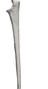
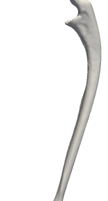
(a) Gauss

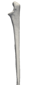
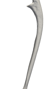
(b) Multiscale (isotropic)

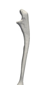
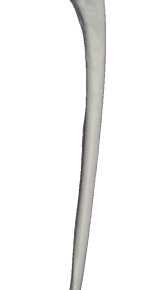
(c) Multiscale (anisotropic)

Figure 9: The effect of varying the first two modes of variation for each model.

Following Styner et al. we evaluate these three models using the standard criteria generalization, specificity and compactness [50]. Generalization refers to the model’s ability to accurately represent all valid instances of the modelled class. We will discuss it in the next subsection. Specificity refers to the model’s ability to only represent valid instances of the modelled bone. It is evaluated by randomly sampling instances of the model and then determining their distance to the closest example of a set of anatomically normal training examples. Compactness, is the accumulated variance for a fixed number of components. This reflects the fact that if two models have the same generalization ability, we would prefer the one with less variance. Table 1 summarizes the specificity and compactness for these models. We evaluated both measures once consider only the first component, and once with the full model. We see the anisotropic model is more specific and more compact than the other models, which means that it should lead to more robust results in practical applications.

Model	Specificity		Compactness
	1st PC	Full model	1st PC	Full model
Gauss	2.6	5.8	50.6	299.1
Isotropic Multiscale	2.3	6.1	51.1	317.0
Anisotropic Multiscale	1.9	2.9	51.1	137.1

Table 1: The specificity and compactness values computed for each of the three models. The lower the specificity and compactness the better.

5.3 Surface registration

To evaluate the generalization ability, we need to determine how well the model can represent valid target shapes, by fitting the model to typical shape surfaces. To fit the model, we use the surface registration algorithm presented in Section 4.1. Figure 10 shows a boxplot with the generalization results. We also see that the multiscale and the anisotropic model lead to similar results, but both outperform model where only a simple Gaussian kernel was used. Since the anisotropic model can fit the models with the same accuracy than the multiscale model, despite being much more compact, means that it is clearly better targeted to the given application. We we will see in the last experiment, this is a big advantage in more complicated registration tasks, such as image to image registration.

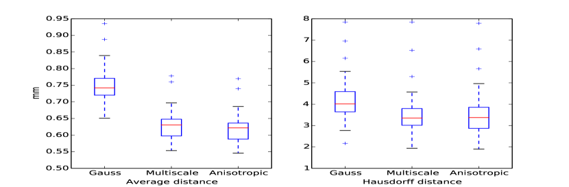
Figure 10: Generalization ability measured by fitting the different models to all ulna surfaces.

5.4 Generalized Active Shape Model fitting

The well known Active Shape Modelling approach [2] can be interpreted as a special case of Gaussian process registration as introduced in Section 4, where the model is a classical SSM (i.e. the sample mean and covariance kernel (11) are used) and an iterative algorithm is used to fit the model to the image. Active Shape Model fitting is a very successful technique for model-based segmentation. Its main drawback is that the solution is restricted to lie in the span of the underlying statistical shape model, which might not be flexible enough to accurately represent the shape. In our case, where we have only 36 datasets of the ulna available, we expect this to be a major problem.

To build an Active Shape Model, we use the fitting results obtained in the previous section together with the original CT images as training data. Besides a standard ASM, we use the techniques for enlarging the flexibility of shape models discussed in Section 3, to build also an extended model with additive smooth deformations (cf. Section 3.3.2), and a “localized“ model (cf. Section 3.3.3). In the first case, we use a Gaussian kernel $k_{g}^{(3,100)}$ to model the unexplained part. Also for localization we choose a Gaussian kernel $k_{g}^{(1,100)}$, but this time with scale 1, in order no to change the variance of the original model. In both cases, we approximate the first 100 eigenfunctions. Figure 11 shows the corresponding fitting result from a leave-one-out experiment. We see that both the extended and the localized model improve the results compared to the standard Active Shape Model. We can also observe that by adding flexibility, the model becomes less robust and the number of outliers (i.e. bad fitting results) increases.

Figure 11: Accuracy of the Active Shape Model fitting algorithm for three different models.

We can remedy that effect by incorporating landmark constraints on the proximal and distal ends, by computing a posterior model (see Section 3.4). This has the effect of fixing the proximal and distal ends and prevents the model from moving away too far from the correct solution. Figure 12 shows that this has the desired effect and the combination of including landmarks and increasing the model flexibility leads to clearly improved results.

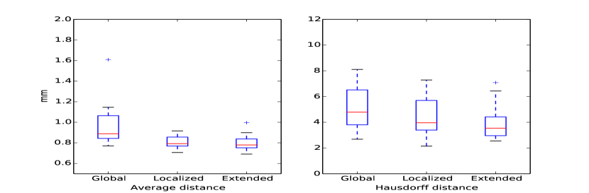
Figure 12: Accuracy of the Active Shape Model fitting algorithm for three different models, when 4 landmarks at the proximal and distal ends were used to make the models more robust.

5.5 Image to image registration

In a last experiment we show that our model can also be used to perform 3D image to image registration, using the full forearm CT images. We choose one image as a reference and build a GPMM on the full image domain. In the application of GPMMs to image registration, we have to be careful about the image borders, as the basis functions are global, and hence values at the boundary might strongly influence values in the interior. We therefore mask the images, and optimize only on the bounding box of the bones. We use a simple mean squares metric and a stochastic gradient descent algorithm to optimize the registration functional (see Equation (18)). To evaluate the method, we warp the ground-truth segmentation of the forearm bones with the resulting deformation field and determine the distance between the corresponding surfaces. Figure 13 shows the results for the same three models as used in the first experiment. In this example, where the optimization task is much more difficult, we see that the anisotropic model, which is much more targeted to the application, has clear advantages.

Figure 13: Accuracy of image to image registration results performed with different models, compared on a ground-truth segmentation of the bones.

We also compared our method to a standard B-Spline registration method [51], which is the standard registration method used in Elastix. First, we use a B-spline that is only defined on a single scale level. As expected, since B-Splines are not application-specific, the result are less robust and the accuracy is worse on average (see Figure 13). In its standard setting, Elastix uses a multi-resolution approach, where it refines the B-Spline grid, in every resolution level. This corresponds roughly to our multiscale approach, but with the important difference that new scale levels are added for each resolution level. This strategy makes the approach much more stable and, thanks to the convenient numerical properties of B-Splines, allows for arbitrarily fine deformations. As shown in Figure 14 in this multi-resolution setting, the B-Spline registration yields more accurate results on average than our method, but, as expected, is less robust.

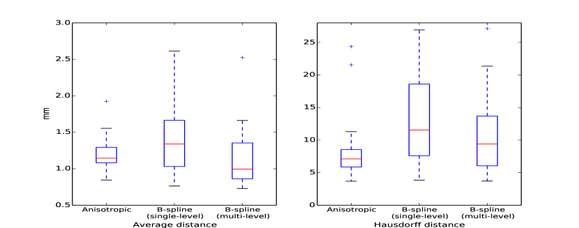
Figure 14: Accuracy of image to image registration results performed with our best model, compared to a single-level and multi-level B-spline registration method implemented in Elastix.

It is interesting to compare the two strategies in more detail. While our model has 500 parameters, the final result of the B-Spline registration has 37926 parameters. Thanks to the convenient numerical properties of B-Splines, more could be added if to increase the model’s flexibility even further. This explains why the B-Spline approach can yield more accurate solutions than GPMMs. With GPMMs, the number of parameters is limited by the number of eigenfunctions we can accurately approximate (see Appendix A for a more detailed discussion). If the image domain is large compared to the scale of the features we need to match, this quickly becomes a limitation. To achieve a similar accuracy as the B-Spline approach, one possibility would be to perform a hierarchical decomposition of the domain and to define more flexible models for each of the smaller subdomains.

6 Conclusion

We have presented Gaussian Process Morphable Models, a generalization of PCA-based statistical shape models. GPMMs extends standard SSMs in two ways: First GPMMs are defined by a Gaussian process, which makes them inherently continuous and do not force an early discretization. More importantly, rather than only estimating the covariances from example datasets, GPMMs can be specified using arbitrary positive definite kernels. This makes it possible to build complex shape priors, even in the case where we do not have many example dataset to learn a statistical shape model. Similar to an SSM, a GPMM is a low-dimensional, parametric model. It can be brought into the exact same mathematical form as an SSM by discretizing the domain on which the model is defined. Hence our generalized shape models can be used in any algorithm that uses a standard shape model. To make our method easily accessible, we have made the full implementation available as part of the open source framework statismo [6] and scalismo [7].

Our experiments have confirmed that GPMMs are ideally suited for modeling prior shape knowlege in registration problems. As all prior assumptions about shape deformations are encoded as part of the GPMM, our approach achieve a clear separation between the modelling and optimization. This separation makes it possible to use the same numerical methods with many different priors. Furthermore, as a GPMM is generative, we can assess the validity of our prior assumptions by sampling from the model. We have shown how the same registration method can be adapted to a wide variety of different applications by simply changing the prior model. Indeed, Gaussian processes give us a very rich modelling language to define this prior, leading to registration methods that can combine learned with generic shape deformations or are spatially varying. From a practitioners point of view, the straight-forward integration of landmarks may also be a valuable contribution, since it enables to develop efficient interactive registration schemes.

The most important assumption behind our models is that the shape variations can be well approximated using only a moderate number of leading basis functions. As shape deformations between objects of the same class are usually smooth and hence the deformations between neighboring points highly correlated, this assumption is usually satisfied. Furthermore for most anatomical shapes, fine detailed deformations only occur in parts of the shape. GPMMs give us the modelling power to model these fine deformations only where they are needed. Our method reaches its limitations, when very fine deformations need to be modelled over a large domain, as it is sometimes required in image registration. In this case the approximation scheme becomes inefficient and the approximations inaccurate. An interesting extension for future work would be to devise a hierarchical, multi-resolution approach, which would partition the domain in order and perform separate approximation on smaller sub-domain. In this way, the modelling power of GPMMs could be exploited to model good priors for image registration, while still offering all the flexibility of classical image registration approaches.

We hope with this work to bridge the gap between the so far distinct world of classical shape modelling, where all the modelled shape variations are a linear combination of the training shapes, and the word of registration, where usually oversimplistic smoothness priors are used. We believe that it is the middle ground between these two extremes, where shape modelling can do most for helping to devise robust and practical applications.

Appendix A Accuracy of the low-rank approximation

The success of our method strongly depends on how well the truncated KL-Expansion

$$\tilde{u}(x)\sim\mu(x)+\sum_{i=1}^{r}\alpha_{i}\sqrt{\lambda}_{i}\phi_{i}(x),\,\alpha_{i}\in\mathcal{N}(0,1),$$ (19)

approximates the full Gaussian process $u\sim GP(\mu,k)$ (cf. Section 2.2). The final approximation error depends on one hand on the error we make by approximating the Gaussian process using the $r$ leading eigenfunctions only, and on the other hand also on how accurately we can compute these eigenfunctions using the Nyström method.

A.1 An analytic example

Before studying these approximations, we illustrate the trade-offs that we face on the example of the Gaussian kernel

$$k(x,y)=\exp(-\lVert x-y\rVert^{2}/\sigma^{2}),$$

for which the eigenfunctions are known. The example is given in Zhu et al. [52], and the discussion is loosely based on a similar investigation by Williams et al. [53]. The eigenvalues $\lambda_{i}$ and eigenfunctions $\phi_{i}$ for $i=1,\ldots,r$ of the integral operator $\mathcal{T}_{k}$ associated to $k$ (cf. Equation (7)), with respect to the distribution $\rho(x)\sim N(0,s^{2})$ are given by,

$$\lambda_{i} =\sqrt{\frac{\pi}{A}}B^{i}$$ (20)

$$\phi_{i}(x) =\exp(-(c-a)x^{2})H_{i}(\sqrt{2c}x)$$ (21)

where $H_{i}$ is the $i-$th order Hermite polynomial, and

$$a^{-1}=4\sigma^{2},\;b^{-1}=s^{2},\;c=\sqrt{a^{2}+2ab},\;$$ (22)

$$A=a+b+c,\;B=b/A.$$ (23)

Figure 15 shows a plot of the first few eigenfunctions. We observe that the eigenfunctions are global, even though the kernels are highly localized. We also observe that the larger the bandwidth $\sigma$ of the Gaussian kernel, the lower the frequency of the leading eigenfunctions. Furthermore, the spectrum decreases more rapidly. Hence, the larger we chose $\sigma$ (i.e. the more smooth the sample functions are) the fewer basis functions we need to accurately represent the full Gaussian process.

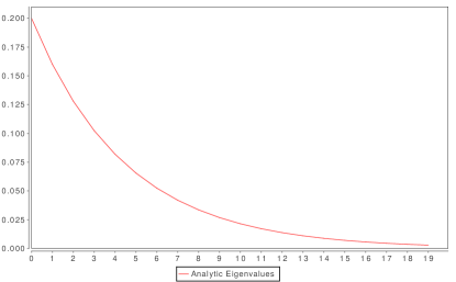
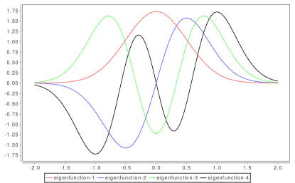
(a)

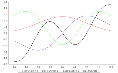
(b)

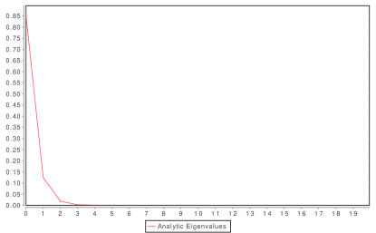
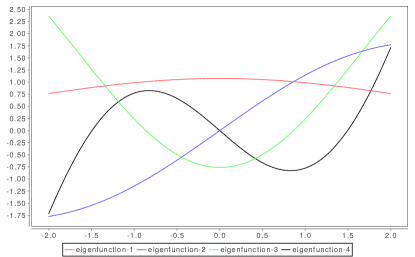
(c)

Figure 15: The first eigenfunctions and the eigenvalues spectrum for $\sigma=0.1$, $\sigma=1.0$ and $\sigma=10.0$.

A similar effect can be observed if we change the support of the domain over which the kernel is defined. In our example, we can simulate an increasing support by changing the variance $s^{2}$ of the probability measure $\rho(x)$. As Figure 16 confirms, the larger we choose $s^{2}$, the faster the eigenvalues decay. We see that it is the ratio between the support of the domain and the smoothness, which determines how many basis functions we need to achieve a good approximation.

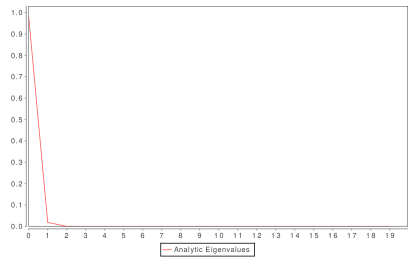
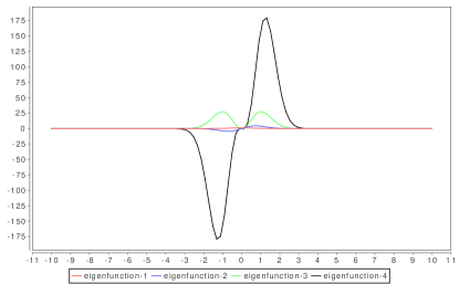
(a)

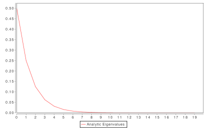
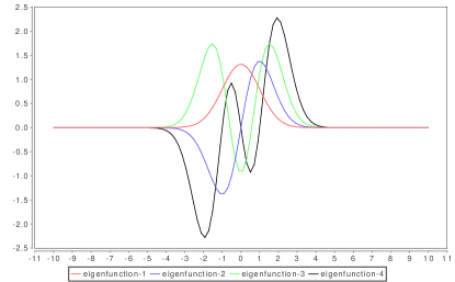
(b)

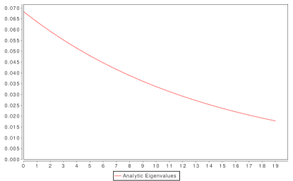
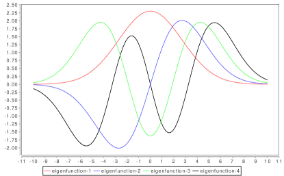
(c)

Figure 16: The first eigenfunctions and the eigenvalues spectrum for different sizes of the support $s^{2}=0.1$, $s^{2}=1.0$ and $s^{2}=10.0$.

While we have only shown it for the Gaussian kernel, it is intuitively clear that similar observations hold for any kernel that enforces smoothness. This can be seen by noting that the more smoothness is enforced by the kernel, the more will the points of the domain vary together. Hence, it is possible to capture more of the variance using only a few basis function.

A.2 Approximation accuracy of the eigenfunction computations

In virtually all practical applications, it is not possible to obtain an analytic expression of the eigenfunctions. Fortunately, it is often possible to obtain good approximations by means of numerical procedures, such as the Nyström approximation that we presented in Section 2.3. Bounds for the quality of this approximation error have recently been given by Rosasco et al. [54]. We repeat here the two main results, which give us an insight on on the main influence factors for the approximation quality, as a function of the number of nystrom points $n$.

Theorem 1 (Rosasco et al. [54])

Let $\mathcal{T}_{k}$ denote the integral operation associated to $k$ and $K$ be the kernel matrix defined by $k_{ij}=k(x_{i},x_{j})$. Further, let $\kappa=\sup_{x\in\Omega}k(x,x)$. There exist an extended enumeration $(\lambda_{i})_{i\geq 1}$ of discrete eigenvalues for $\mathcal{T}_{k}$ and an extended enumeration $(\hat{\lambda}_{i})_{i\geq 1}$ of discrete eigenvalues of $K$ such that

$$\sum_{i\geq 1}(\lambda_{i}-\hat{\lambda}_{i})^{2}\leq\frac{8\kappa^{2}\tau}{n}$$

with confidence greater than $1-2\exp{\tau}$. In particular

$$\sup_{i\geq 1}\lvert\lambda_{i}-\hat{\lambda}_{i}\rvert\leq\frac{2\sqrt{2}\kappa\sqrt{\tau}}{\sqrt{n}}.$$

Theorem 2 (Rosasco et al. [54])

Given an integer $N$, let $m$ be the sum of the multiplicities of the first $N$ distinct eigenvalues of $\mathcal{T}_{K}$, so that

$$\lambda_{1}\geq\lambda_{2}\geq\ldots,\geq\lambda_{m}\geq\lambda_{m+1},$$

and $P_{N}$ be the orthogonal projection from $L^{2}(\Omega,\rho)$ onto the span of the corresponding eigenfunctions. Let $r$ be the rank of $K$, and $\hat{u}_{1},\ldots,\hat{u}_{k}$ the eigenvectors corresponding to the nonzero eigenvalues of $K$ in a decreasing order. Denote by $\hat{v}^{1},\ldots,\hat{v}^{k}\subset L^{2}(\Omega,\rho)$ the corresponding Nyström extension. Given $\tau>0$ if the number $n$ of examples satisfies

$$n>\frac{128\kappa^{2}\tau}{(\lambda_{m}-\lambda_{m+1})^{2}}$$

then

$$\sum_{j=1}^{m}\lVert(I-P_{N})\hat{v_{j}}\rVert_{\rho}^{2}+\sum_{j=m+1}^{r}\lVert P_{N}\hat{v}_{j}\rVert_{\rho}^{2}\leq\frac{32\kappa^{2}\tau}{(\lambda_{m}-\lambda_{m+1})^{2}n},$$

with probability greater than $1-2\exp{-\tau}$.

While these bounds are too loose to use them in practical applications, they have a number of important implications. First, we note that these theorems hold for an arbitrary distribution. Hence, independently of whether we sample the points for the Nyström approximation from the surface, or in a volume, we know that convergence is always guaranteed if the number of points $n$ is sufficiently large. Second, the bound on the eigenvalues (1) does not depend on the smoothness induced by the kernel, nor does it depend on the support of the domain. Hence, for a given $n$ we have a guaranteed accuracy independent of the smoothness induced by the kernel. Third, the main factor that influences the projection error (Theorem 2) is how fast the eigenvalues $\lambda_{m}-\lambda_{m+1}$ decay. As more smooth functions imply faster decay, this implies that we need fewer points for the approximation when the kernel induces more smoothness.

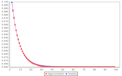
(a) Spectrum $(n=200)$

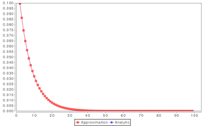
(b) Spectrum $(n=1000)$

(c) $\phi_{1}:n=200$

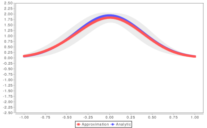
(d) $\phi_{1}:n=1000$

(e) $\phi_{10}:n=200$

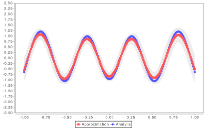
(f) $\phi_{10}:n=1000$

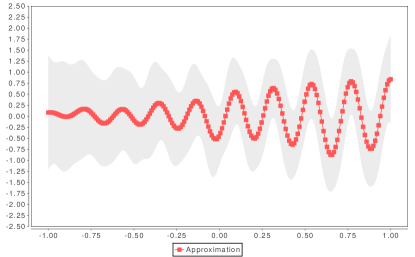
(g) $\phi_{40}:n=200$

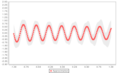
(h) $\phi_{40}:n=1000$

Figure 17: Estimation of the eigenvalues and eigenfunctions. The plots show the average and standard-deviation estimated from 100 runs, with parameters $\sigma=1$ and $\sigma=0.2$. The blue line shows the analytic solution. (The analytic solution for $\phi_{40}$ is not available, as the numeric computation of the $40-$th hermite polynomial is not feasible.)

Figure 17 shows approximations of the eigenvalues and eigenfunctions for the case where $\sigma=1$ and $\sigma=0.2$. We see that the eigenvalues are extremely well approximated, even for $n=200$. As the bound for the eigenfunctions predicts, the eigenfunctions are approximated reasonably well as long as the spectrum decays quickly. Where the decay is slow (i.e. for eigenfunction $\phi_{40}$ the approximation with $n=200$ is not good enough anymore and more points need to be chosen to obtain a reasonable approximation. In this case, $n=1000$ leads to a satisfactory approximation. We also see in this example that the bounds are much too pessimistic. For $n=200$, Theorem 1 asserts that with probability $0.99$, the largest difference between the true and the approximated eigenvalues $\sup_{j}(\lambda_{j}-\hat{\lambda}_{j})$ for $n=200$ is $0.48$ and for $n=1000$ is $0.2$, where in reality the values are at least an order of magnitude better.

A.3 Choosing the approximation parameters

The above considerations allow us to come up with an approach of choosing the parameters for the approximation. We suggest the following procedure:

1. Define a Gaussian process model $\mathcal{GP}(\mu,k)$, which represents the prior knowledge

2. Determine the total variance that should be covered by the approximation

3. Compute from the eigenvalues the number of eigenfunctions $r$ that are needed to retain a certain fraction of the variance, such that the desired fraction of variance $p$ from the total variance $var(k)$ is retained, i.e.

   $$r=\operatornamewithlimits{arg\,min}_{m}\frac{\sum_{j=1}^{m}\hat{\lambda}_{j}}{var(k)}>p.$$

4. Choose the number of points that we need for the Nyström approximation, such that the $i-$th eigenfunction, for which $\lambda_{i}-\lambda_{i+1}$ is minimal, leads to a stable approximation.

The total variance $var(k)$ in step 3 can be estimated by noting that

$$var(k)=\sum_{i=1}^{\infty}\lambda_{i}=\int_{\Omega}k(x,x)\,dp(x),$$

and use numerical integration to estimate the value of the integral. For stationary kernels, this last step can even be avoided, by noting that $k(x,x)$ is constant and hence the total sum is simply $k(x,x)$ for some $x\in\Omega$. For estimating the leading eigenvalues, we use the Nyström approximation, for which we know that it can accurately estimate the eigenvalues. Choosing the number of points for the Nyström approximation (step 4) is more difficult. The bound given in Theorem 2 is not tight enough to be of practical use. To determine whether we have chosen sufficiently many points for the Nyström approximation, we propose the following experiment: We define the full Gaussian process $\mathcal{GP}(\mu,k)$ and draw random samples for a discrete number of points $x_{1},\ldots,x_{N}\subset\Omega$, toobtain the sample values $\hat{u}(x_{1}),\ldots,\hat{u}(x_{N})$. This can be done by sampling from the multivariate normal distribution, $\mathcal{N}(\mu,K)$, where K is the Kernel matrix $K_{ij}=k(x_{i},x_{j}),\;i,j=1\ldots,N$. The overall error of the low rank approximation can be assessed by determining how well we can approximate the samples with the low-rank Gaussian process $\mathcal{GP}(\mu,\tilde{k})$. This can be efficiently done by performing a Gaussian process regression with training data $\{(x_{1},\hat{u}(x_{1}),\ldots,(x_{N},\hat{u}(x_{N})\}$ (see e.g. [13], Chapter 2 for details). Figure 18 shows this approach for a 1D example. We have tested an approximation that covers $99\%$ of the variance for different kernels. The error was estimated using $1000$ points of the domain. We see that for $\sigma=0.005$, for which the sample is very wiggly (Figure 18a), the approximation error is slightly larger than the $1\%$, and hence we would need to increase the number of points used for the Nyström approximation. For all other kernels, the error is very close or even below the desired $1\%$ approximation error. That the value is sometimes smaller than $1\%$ is because the eigenvalues are discrete, and hence we might actually cover more than $99\%$ by choosing the $r$ first eigenfunctions.

(a) $\sigma=0.005$

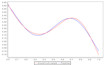
(b) $\sigma=0.5$

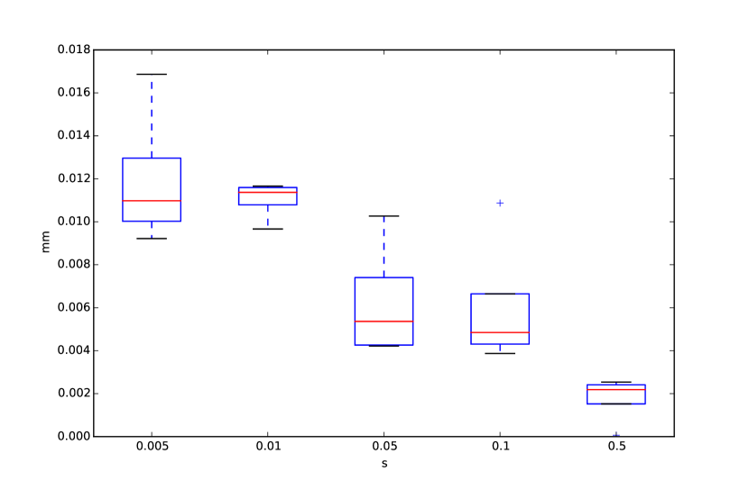
(c)

Figure 18: LABEL:sub@fig:sample-gpwiggly, LABEL:sub@fig:sample-gpsmooth: Random samples from the Gaussian process with kernel $k(x,x^{\prime})=\exp({-\lVert x-x^{\prime}/\sigma^{2}\rVert})$, for $\sigma=0.005$ and $\sigma=0.5$. LABEL:sub@fig:overall-error-estimate The projection error of random samples when using a low-rank approximation that covers $99\%$ of the variance. We see that despite the various numerical approximations, the desired approximation error of $0.01$ is attained even for functions that enforce very little smoothness.

References

- [1] U. Grenander and M. I. Miller, Pattern theory: from representation to inference. Oxford university press Oxford, 2007, vol. 1.
- [2] T. F. Cootes, C. J. Taylor, D. H. Cooper, J. Graham, and others, “Active shape models-their training and application,” Computer Vision and Image Understanding, vol. 61, no. 1, 1995.
- [3] V. Blanz and T. Vetter, “A morphable model for the synthesis of 3d faces,” in SIGGRAPH ’99: Proceedings of the 26th annual conference on Computer graphics and interactive techniques. ACM Press, 1999, pp. 187–194.
- [4] M. Li and J. T.-Y. Kwok, “Making large-scale nystrom approximation possible,” 2010.
- [5] A. Myronenko and X. Song, “Point set registration: Coherent point drift,” Pattern Analysis and Machine Intelligence, IEEE Transactions on, vol. 32, no. 12, pp. 2262–2275, 2010.
- [6] M. Lüthi, R. Blanc, T. Albrecht, T. Gass, O. Goksel, P. Büchler, M. Kistler, H. Bousleiman, M. Reyes, P. C. Cattin, and others, “Statismo-a framework for PCA based statistical models.” Insight Journal, 2012.
- [7] “Scalismo - scalable image analysis and shape modelling,” http://github.com/unibas-gravis/scalismo.
- [8] Y. Wang and L. H. Staib, “Boundary finding with prior shape and smoothness models,” IEEE Transactions on Pattern Analysis and Machine Intelligence, vol. 22, no. 7, 2000.
- [9] U. Grenander and M. I. Miller, “Computational anatomy: An emerging discipline,” Quarterly of applied mathematics, vol. 56, no. 4, pp. 617–694, 1998.
- [10] Y. Amit, U. Grenander, and M. Piccioni, “Structural image restoration through deformable templates,” Journal of the American Statistical Association, vol. 86, no. 414, pp. 376–387, 1991.
- [11] S. C. Joshi, A. Banerjee, G. E. Christensen, J. G. Csernansky, J. W. Haller, M. I. Miller, and L. Wang, “Gaussian random fields on sub-manifolds for characterizing brain surfaces,” in Information Processing in Medical Imaging. Springer, 1997, pp. 381–386.
- [12] M. Holden, “A review of geometric transformations for nonrigid body registration,” IEEE TRANSACTIONS ON MEDICAL IMAGING, vol. 27, no. 1, p. 111, 2008.
- [13] C. E. Rasmussen and C. K. Williams, Gaussian processes for machine learning. Springer, 2006.
- [14] J. Zhu, S. C. Hoi, and M. R. Lyu, “Nonrigid shape recovery by gaussian process regression,” in Computer Vision and Pattern Recognition, 2009. CVPR 2009. IEEE Conference on. IEEE, 2009, pp. 1319–1326.
- [15] B. Schölkopf, F. Steinke, and V. Blanz, “Object correspondence as a machine learning problem,” in ICML ’05: Proceedings of the 22nd international conference on Machine learning. New York, NY, USA: ACM Press, 2005, pp. 776–783.
- [16] L. Younes, Shapes and diffeomorphisms. Springer, 2010, vol. 171.
- [17] M. Bruveris, L. Risser, and F.-X. Vialard, “Mixture of kernels and iterated semidirect product of diffeomorphisms groups,” Multiscale Modeling & Simulation, vol. 10, no. 4, pp. 1344–1368, 2012.
- [18] S. Sommer, F. Lauze, M. Nielsen, and X. Pennec, “Sparse multi-scale diffeomorphic registration: the kernel bundle framework,” Journal of mathematical imaging and vision, vol. 46, no. 3, pp. 292–308, 2013.
- [19] T. Schmah, L. Risser, and F.-X. Vialard, “Left-invariant metrics for diffeomorphic image registration with spatially-varying regularisation,” in Medical Image Computing and Computer-Assisted Intervention–MICCAI 2013. Springer, 2013, pp. 203–210.
- [20] T. F. Cootes and C. J. Taylor, “Combining point distribution models with shape models based on finite element analysis,” Image and Vision Computing, vol. 13, no. 5, 1995.
- [21] Z. Zhao, S. R. Aylward, and E. K. Teoh, “A novel 3d partitioned active shape model for segmentation of brain mr images,” in Medical Image Computing and Computer-Assisted Intervention–MICCAI 2005. Springer, 2005, pp. 221–228.
- [22] C. Davatzikos, X. Tao, and D. Shen, “Hierarchical active shape models, using the wavelet transform,” Medical Imaging, IEEE Transactions on, vol. 22, no. 3, pp. 414–423, 2003.
- [23] D. Nain, S. Haker, A. Bobick, and A. Tannenbaum, “Multiscale 3-d shape representation and segmentation using spherical wavelets,” Medical Imaging, IEEE Transactions on, vol. 26, no. 4, pp. 598–618, 2007.
- [24] T. Albrecht, M. Lüthi, and T. Vetter, “A statistical deformation prior for non-rigid image and shape registration,” in Computer Vision and Pattern Recognition, 2008. CVPR 2008. IEEE Conference on. IEEE, 2008, pp. 1–8.
- [25] D. Kainmueller, H. Lamecker, M. O. Heller, B. Weber, H.-C. Hege, and S. Zachow, “Omnidirectional displacements for deformable surfaces,” Medical image analysis, vol. 17, no. 4, pp. 429–441, 2013.
- [26] Y. Le, U. Kurkure, and I. Kakadiaris, “PDM-ENLOR: Learning ensemble of local PDM-based regressions,” in 2013 IEEE Conference on Computer Vision and Pattern Recognition (CVPR), Jun. 2013, pp. 1878–1885.
- [27] M. Lüthi, C. Jud, and T. Vetter, “Using landmarks as a deformation prior for hybrid image registration,” Pattern Recognition, pp. 196–205, 2011.
- [28] T. Gerig, K. Shahim, M. Reyes, T. Vetter, and M. Lüthi, “Spatially varying registration using gaussian processes,” in Medical Image Computing and Computer-Assisted Intervention–MICCAI 2014. Springer, 2014, pp. 413–420.
- [29] M. Lüthi, C. Jud, and T. Vetter, “A unified approach to shape model fitting and non-rigid registration,” in Machine Learning in Medical Imaging. Springer, 2013, pp. 66–73.
- [30] I. Jolliffe, Principal component analysis. Wiley Online Library, 2002.
- [31] A. Berlinet and C. Thomas-Agnan, Reproducing kernel Hilbert spaces in probability and statistics. Springer, 2004, vol. 3.
- [32] N. Halko, P.-G. Martinsson, and J. A. Tropp, “Finding structure with randomness: Probabilistic algorithms for constructing approximate matrix decompositions,” SIAM review, vol. 53, no. 2, pp. 217–288, 2011. [Online]. Available: http://epubs.siam.org/doi/abs/10.1137/090771806
- [33] D. Duvenaud, “Automatic model construction with gaussian processes,” Ph.D. dissertation, University of Cambridge, 2014.
- [34] P. Paysan, R. Knothe, B. Amberg, S. Romdhani, and T. Vetter, “A 3d face model for pose and illumination invariant face recognition,” in Advanced Video and Signal Based Surveillance, 2009. AVSS’09. Sixth IEEE International Conference On. IEEE, 2009, pp. 296–301.
- [35] M. H. Davis, A. Khotanzad, D. P. Flamig, and S. E. Harms, “Elastic body splines: a physics based approach to coordinate transformation in medical image matching,” in Computer-Based Medical Systems, 1995., Proceedings of the Eighth IEEE Symposium on. IEEE, 1995, pp. 81–88.
- [36] J. Kybic and M. Unser, “Fast parametric elastic image registration,” Image Processing, IEEE Transactions on, vol. 12, no. 11, pp. 1427–1442, 2003.
- [37] K. Rohr, H. S. Stiehl, R. Sprengel, T. M. Buzug, J. Weese, and M. Kuhn, “Landmark-based elastic registration using approximating thin-plate splines,” Medical Imaging, IEEE Transactions on, vol. 20, no. 6, pp. 526–534, 2001.
- [38] J. Shawe-Taylor and N. Cristianini, Kernel methods for pattern analysis. Cambridge university press, 2004.
- [39] R. Opfer, “Multiscale kernels,” Advances in Computational Mathematics, vol. 25, no. 4, pp. 357–380, 2006.
- [40] Y. Xu and H. Zhang, “Refinement of reproducing kernels,” The Journal of Machine Learning Research, vol. 10, pp. 107–140, 2009.
- [41] G. Wahba, Spline models for observational data. Society for Industrial Mathematics, 1990.
- [42] A. Sotiras, C. Davatzikos, and N. Paragios, “Deformable medical image registration: A survey,” Medical Imaging, IEEE Transactions on, vol. 32, no. 7, pp. 1153–1190, 2013.
- [43] S. Klein, M. Staring, and J. P. Pluim, “Evaluation of optimization methods for nonrigid medical image registration using mutual information and b-splines,” Image Processing, IEEE Transactions on, vol. 16, no. 12, pp. 2879–2890, 2007.
- [44] H. J. Johnson and G. E. Christensen, “Consistent landmark and intensity-based image registration,” Medical Imaging, IEEE Transactions on, vol. 21, no. 5, pp. 450–461, 2002.
- [45] B. Fischer and J. Modersitzki, “Combination of automatic non-rigid and landmark based registration: the best of both worlds,” Medical imaging, pp. 1037–1048, 2003.
- [46] A. Biesdorf, S. W\örz, H. J. Kaiser, C. Stippich, and K. Rohr, “Hybrid spline-based multimodal registration using local measures for joint entropy and mutual information,” Medical Image Computing and Computer-Assisted Intervention–MICCAI 2009, pp. 607–615, 2009.
- [47] W. E. Lorensen and H. E. Cline, “Marching cubes: A high resolution 3d surface construction algorithm,” in ACM siggraph computer graphics, vol. 21, no. 4. ACM, 1987, pp. 163–169.
- [48] S. Umeyama, “Least-squares estimation of transformation parameters between two point patterns,” IEEE Transactions on Pattern Analysis & Machine Intelligence, no. 4, pp. 376–380, 1991.
- [49] S. Klein, M. Staring, K. Murphy, M. Viergever, J. Pluim et al., “Elastix: a toolbox for intensity-based medical image registration,” IEEE transactions on medical imaging, vol. 29, no. 1, pp. 196–205, 2010.
- [50] M. A. Styner, K. T. Rajamani, L.-P. Nolte, G. Zsemlye, G. Székely, C. J. Taylor, and R. H. Davies, “Evaluation of 3d correspondence methods for model building,” in Information processing in medical imaging. Springer, 2003, pp. 63–75.
- [51] D. Rueckert, A. F. Frangi, and J. A. Schnabel, “Automatic construction of 3d statistical deformation models using non-rigid registration,” in MICCAI ’01: Medical Image Computing and Computer-Assisted Intervention, 2001, pp. 77–84.
- [52] H. Zhu, C. K. Williams, R. Rohwer, and M. Morciniec, “Gaussian regression and optimal finite dimensional linear models,” Neural Networks and Machine Learning, 1998.
- [53] C. Williams and M. Seeger, “The effect of the input density distribution on kernel-based classifiers,” in Proceedings of the 17th International Conference on Machine Learning, 2000, pp. 1159–1166.
- [54] L. Rosasco, M. Belkin, and E. D. Vito, “On learning with integral operators,” The Journal of Machine Learning Research, vol. 11, pp. 905–934, 2010. [Online]. Available: http://dl.acm.org/citation.cfm?id=1756036