Numerical Modeling of the Early Light Curves of Type IIP Supernovae

Abstract

The early rise of Type IIP supernovae (SN IIP) provides important information for constraining the properties of their progenitors. This can in turn be compared to pre-explosion imaging constraints and stellar models to develop a more complete picture of how massive stars evolve and end their lives. Using the SuperNova Explosion Code (SNEC), we model the first $40$ days of SNe IIP to better understand what constraints can be derived from their early light curves. We use two sets of red supergiant progenitor models with zero-age main sequence masses in the range between $9\,M_{\odot}$ and $20\,M_{\odot}$. We find that the early properties of the light curve depend most sensitively on the radius of the progenitor, and thus provide a relation between the $g$-band rise time and the radius at the time of explosion. This relation will be useful for deriving constraints on progenitors from future observations, especially in cases where detailed modeling of the entire rise is not practical. When comparing to observed rise times, the radii we find are a factor of a few larger than previous semi-analytic derivations and generally in better agreement with what is found with current stellar evolution calculations.

1. Introduction

One of the outstanding problems in astrophysics is connecting the variety of core-collapse supernovae (SNe) we observe with the massive progenitors that give rise to them. Ideally, we would use pre-explosion imaging to directly identify these progenitors (e.g., Van Dyk et al., 2012; Smartt et al., 2009; Li et al., 2006). Unfortunately, in most cases such information is not available because the progenitor is too dim or deep pre-explosion imaging is not available at the needed location. For this reason, features of the early light curves can be especially helpful in constraining progenitor properties (Piro & Nakar, 2013). Emission dominated by shock cooling should reflect the radius of the exploding star (Nakar & Sari 2010, hereafter NS10). Furthermore, the presence of extended material (Nakar & Piro, 2014; Piro, 2015) and the interaction with a companion (Kasen, 2010) can create additional features that teach us about how massive stars end their lives.

This early phase has been explored in a number of theoretical works semi-analytically (e.g., NS10; Piro et al. 2010; Rabinak & Waxman 2011). These studies generally took the approach of assuming an idealized (i.e., polytropic) density profile for the star to make connections between early light curve properties and the properties of the star in a general way. The question though is whether in nature such idealized profiles actually occur at relevant depths within the star. On the other hand, numerical models represent a powerful complementary approach to analytic studies of SN light curves, including the early phases (see Eastman et al., 1994; Young, 2004; Kasen & Woosley, 2009; Bersten et al., 2011; Dessart et al., 2013). For example, Bersten et al. (2012) constrained the radius of the progenitor star for SN 2011dh based on the numerical modeling of its early light curve. In this case, many of these calculations are tailored for specific events. This makes it difficult to generalize these results more broadly, which would be especially useful as current and future transient surveys (e.g., iPTF/ZTF, ASAS-SN, BlackGEM, Pan-STARRS, LSST) find larger samples of SNe.

Motivated by these issues, we undertake a numerical exploration of how rise times of SNe IIP vary with the parameters of their progenitors. We utilize two sets of nonrotating solar-metallicity progenitor models from the stellar evolution codes MESA (Paxton et al., 2011, 2013, 2015) and KEPLER (Weaver et al., 1978; Woosley & Heger, 2007; Sukhbold & Woosley, 2014; Woosley & Heger, 2015), and explode these models and generate light curves using the SuperNova Explosion Code (SNEC; Morozova et al. 2015). We describe important differences between realistic stellar models and more idealized treatments, and how these impact observable features of the early light curves. In addition, based on the results of our numerical models, we derive a relation for the rise time $t_{\rm rise}$ of SN IIP light curves in $g$-band as a function of the radius $R$ of the progenitor. This relation may be useful in the future analyses of observed early rises, especially when comparing large samples of events.

The paper is organized as follows. In Section 2, we describe the progenitor models used in this study and the numerical setup of our simulations. In Section 3, we discuss two important aspects of our calculations related to the stellar models and radiative diffusion. This highlights differences with more idealized treatments. In Section 4, we present our full set of explosion models and summarize how the properties of the light curve rise relate to the radius and ejecta mass. In Section 5, we summarize our main results and discuss future work.

2. Numerical setup

This work is primarily focused on SNe IIP, and thus we only consider red supergiant (RSG) progenitor models since these are the observationally-confirmed SN IIP progenitors (see e.g., Smartt et al., 2009; Fraser et al., 2012; Maund et al., 2013). We consider two sets of nonrotating solar-metallicity pre-collapse RSG models. The first set of models comes from the stellar evolution code KEPLER (Woosley & Heger, 2007, 2015; Sukhbold & Woosley, 2014; Sukhbold et al., 2016) and has zero-age main sequence (ZAMS) masses in the range between $9\,M_{\odot}$ and $20\,M_{\odot}$ in steps of $0.5\,M_{\odot}$. We refer the reader to Sukhbold et al. (2016) for a detailed description of these models. The second set of the models we generate using the stellar evolution code MESA (Paxton et al., 2011, 2013, 2015), revision 7624. These models have ZAMS masses in the range between $11\,M_{\odot}$ and $20\,M_{\odot}$ in steps of $0.5\,M_{\odot}$. Our calculation use the same parameter set described in Morozova et al. (2015). We summarize for completeness the parameters that influence more directly the radius determination. We use the 21-isotope nuclear reaction network approx21.net, and use the Ledoux criterion for convection, following Sukhbold & Woosley (2014) for the choice of the free parameters. This corresponds to a mixing length parameter $\alpha_{\mathrm{mlt}}=2.0$, exponentially decreasing overshooting (both for the core and the convective shells) with $f_{\mathrm{ov}}=0.025$ and $f_{0}=0.05$ (see Paxton et al., 2011), and semiconvection efficiency $\alpha_{\mathrm{sc}}=0.1$. Wind mass loss is included as in Morozova et al. (2015), using the “Dutch” mass loss algorithm without any modifying efficiency factor. We set mesh_delta_coeff = mesh_delta_coeff_for_highT = 1.0 for the spatial resolution, and varcontrol_target = $10^{-4}$ for the temporal resolution. We note that experiments with MESA show that the pre-collapse RSG radius depends sensitively on wind efficiency (Renzo et al., in preparation), overshooting, and mixing-length parameters. Generally speaking, the higher the wind efficiency, the more mass is removed and the smaller the radius. The larger $f_{\mathrm{ov}}$, the more massive and luminuous the He core and the larger the radius. The larger $\alpha_{\mathrm{mlt}}$, the more efficient the energy transport through the envelope and the smaller the radius (cf. also Dessart et al. 2013). Ultimately, 3D radiation-hydrodynamic models will be needed to robustly predict RSG radii, e.g., Chiavassa et al. (2009).

Figure 1 summarizes the main features of the considered progenitor models, the radii and masses at the onset of core collapse. The KEPLER models show a strong correlation between radius and mass. We emphasize that whether or not one set of models is more “correct” (in the sense that it is a closer representation of what actually occurs in nature) is irrelevant to our work. The reason is that we are looking for general trends that are satisfied by the explosion of any stellar model (as we will summarize in Section 4). The fact that so much diversity is seen in Figure 1 is actually a strength and not a weakness for our study.

All the stellar models are exploded with SNEC, which is described in detail in Morozova et al. (2015). We excise the inner $1.4\,M_{\odot}$ of the models, assuming that this part collapses and forms a neutron star. Later in the paper, the ejecta mass, $M_{\rm ej}$, is defined as the total stellar mass at core collapse minus $1.4\,M_{\odot}$. We do not model the fallback of material onto the remnant. For the current study, we use a thermal bomb mechanism for the explosion with a duration of $0.001\,{\rm s}$ and a spread of $0.02\,M_{\odot}$ (the choice of bomb duration is discussed in Section 4). We define the final energy, $E_{\rm fin}$, as the final (asymptotic) explosion energy of the model. Note that $E_{\mathrm{fin}}$ is not equal to the energy of the thermal bomb that we use to initiate explosion. The latter is equal to the difference between $E_{\rm fin}$ and the total (mostly gravitational) energy of the progenitor before explosion. We point out that the absolute value of the initial gravitational energy of our models can be of the same order or even larger than $E_{\rm fin}$. “Boxcar” smoothing of the compositional profiles is performed as in Morozova et al. (2015) and the same values for the opacity floor are used. We do not include radioactive ${}^{56}{\rm Ni}$ in our models, since it does not impact these early phases. The numerical gridding of each model is identical to that used in Morozova et al. (2015) and consists of $1000$ cells in mass coordinate. However, for a special case described in Section 3, we use a grid consisting of $2000$ cells, with increasing resolution toward the surface and the center of the models. All light curves are generated for the first $40$ days after explosion.

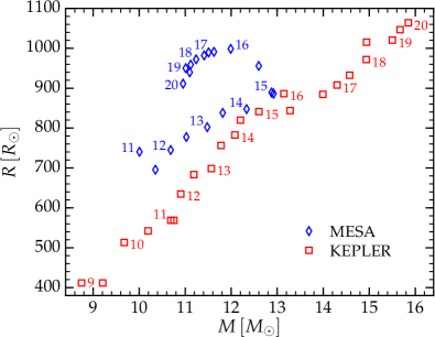
Figure 1.— Radii of the progenitor models versus total masses at the onset of core collapse for both KEPLER and MESA sets. The numbers give the ZAMS masses of the models in units of $M_{\odot}$. In-between models are not labeled to avoid clutter.

3. Key factors determining early light curves

Before presenting our full set of explosion calculations, it is helpful to discuss some of the key aspects of the stellar models and the properties of the radiative diffusion that determine the rising light curves we find. The two main factors we focus on are the shallow density profile of RSGs and the time-dependent position of the so-called luminosity shell. The location of the luminosity shell is the depth from which photons diffuse to reach the photosphere at a given time after shock breakout. These two issues are very connected, since the density profile determines how the shock accelerates and will eventually set the depth of the luminosity shell as shock cooling sets in.

3.1. Density profiles of RSGs

RSGs have convective envelopes, which means that nominally their density $\rho$ obeys the power-law $\rho\propto(R-r)^{n}$, where $r$ is the distance from the center of the star, $R$ is the radius of the star, and $n=1.5$. For this reason, previous analytic studies paid special attention to density profiles with $n=1.5$ (see Matzner & McKee, 1999; Rabinak & Waxman, 2011, NS10). To test this assumption, we plot in Figure 2 $\log_{10}\rho$ as a function of $\log_{10}(R-r)$ for a representative subset of the models described in Section 2. The rest of the models have a similar structure and they are not plotted for clarity. Black dashed lines show fits of the power-laws $\rho\propto(R-r)^{n}$ to different regions of each profile. The indices $n_{1}$ and $n_{2}$ give the power-law exponents obtained for the outer and inner parts of the profile, respectively. The innermost and outermost boundary of the fits for each model are chosen in such a way, that the inner power-law exponent is $1.5$ for all models since the bulk of the envelope is clearly convective.

From the comparison shown in Figure 2, there are multiple key points to take away. First, indeed at sufficiently large depths within the envelope the density profile obeys an $n=1.5$ polytrope. Second, in both MESA and KEPLER models, the outer density profile is different from $n=1.5$ and in general shallower (although at sufficiently short distances to the surface the KEPLER models are steeper, these regions do not impact the light curves we study). This region can cover a few hundred solar radii. Whether or not the shallow profile region has an important impact on the rise depends on the depth where photons are diffusing from during the shock cooling phase. We address this next.

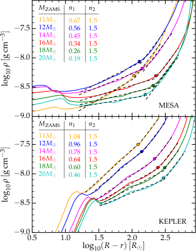
Figure 2.— Example density profiles for some of the considered pre-collapse RSG models. Black dashed lines show the $\rho\propto(R-r)^{n}$ ($R$ is the stellar radius and $r$ is the distance of the location from the center of the star) fits to different regions of the profiles. The variables $n_{1}$ and $n_{2}$ are the power-law exponents of the outer and inner parts of the profiles, respectively. Colored circles separate the two regions with different power-law exponents.

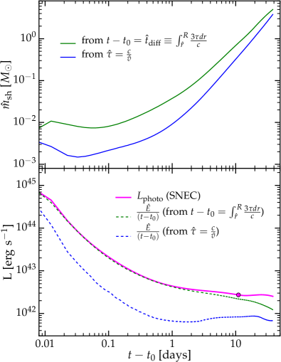
Figure 3.— Top panel: $\hat{m}_{\rm sh}$, the difference between the total mass of the model and the mass coordinate of the luminosity shell, as a function of time since shock breakout ($t_{0}$) for a MESA progenitor model with $M_{\rm ZAMS}=14\,M_{\odot}$ and $E_{\rm fin}=10^{51}\,{\rm erg}$. $\hat{m}_{\mathrm{sh}}$ is computed either via the detailed diffusion time estimate in Equation (1) or via the simpler estimate in Equation (3), using $\hat{\tau}=c/\hat{v}$. Bottom panel: Bolometric luminosities of the same model, computed in three different ways, as described in Section 3.2. The colored circle indicates the time when the luminosity shell found via $\hat{t}_{\rm diff}=t-t_{0}$ enters the convective ($n=1.5$) region of the envelope. Note that the SNEC run used to create this figure was carried out with 2000 cells in mass coordinate.

3.2. Position of the luminosity shell

The shock-cooling phase (from a few to $\sim 20$ days) and the plateau phase (from $\sim 20$ to $\sim 100$ days) of SNe IIP light curves are powered by the energy of the post-explosion shock wave. This energy diffuses out of the expanding envelope and at each moment of time we see the photons coming from the luminosity shell. The position of the luminosity shell at time $t$ is defined by the condition $\hat{t}_{\rm diff}=t-t_{0}$, where $t_{0}$ is the time of shock breakout, $t_{\rm diff}=t_{\rm diff}(r,t)$ is the diffusion time at each time at each depth, and the hat indicates the value of this quantity taken specifically at the luminosity shell. Once the position of the luminosity shell is found, the observed bolometric luminosity can be estimated as $\hat{E}/(t-t_{0})$, where $\hat{E}$ is the internal energy of the luminosity shell.

Given the relatively shallow outer-envelope density profiles we find in realistic stellar models, we explore where the luminosity depth is at each time. In integral form, the diffusion time at the luminosity shell is

$$\hat{t}_{\rm diff}=\int_{\hat{r}}^{R}\frac{3\tau dr}{c}\ ,$$ (1)

where

$$\tau(r)=\int_{r}^{R}\kappa\rho dr\ .$$ (2)

The top panel of Figure 3 shows the position (in mass coordinate) of the luminosity shell found in our calculations for the MESA model with $M_{\rm ZAMS}=14\,M_{\odot}$ and final energy $E_{\rm fin}=10^{51}\,{\rm erg}$. The radius of this model is $R=848\,R_{\odot}$ and the ejecta mass is $M_{\rm ej}=10.93\,M_{\odot}$. The plotted quantity $\hat{m}_{\rm sh}$ is the difference between the total mass of the model and the mass coordinate of the luminosity shell as a function of time. The green curve finds $\hat{m}_{\rm sh}$ using our integral definition for $\hat{t}_{\rm diff}$ given in Equation (1). From this, one can see where photons are diffusing from at a given time. The blue curve finds $\hat{m}_{\rm sh}$ using the condition $\hat{\tau}=c/\hat{v}$ for defining the luminosity shell, where $v$ is the velocity of matter. This alternative relation (in comparison with the integral we use in Equation 1) arises from simplifying the integral definition for the diffusion time by taking

$$t_{\rm diff}\approx\frac{\hat{\tau}\hat{d}}{c}\ ,$$ (3)

where $\hat{d}$ is the width of the luminosity shell, and then setting $\hat{d}=\hat{v}(t-t_{0})$. This simpler description is often used in analytic and semi-analytic works (NS10; Piro 2012, and references therein). In general, the integrated diffusion depth is larger at any given time. This is because the relatively shallow density profile of realistic models makes the full integral crucial for deriving the optical depth. In contrast, if the density profile was steeper, only the conditions at the luminosity depth would really be important and the integral would not be as important.

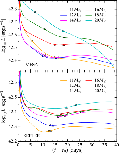
Figure 4.— Bolometric light curves of the MESA (top panel) and KEPLER (bottom panel) models from Figure 2 for a final explosion energy of $E_{\rm fin}=10^{51}\,{\rm erg}$. Colored circles indicate times when the luminosity shell (found via $\hat{t}_{\rm diff}=t-t_{0}$ and Equation 1) enters the convective region of each envelope. Colored triangles roughly indicate when recombination begins (i.e. when effective temperature of the radiation drops down to $7500\,{\rm K}$).

The bottom panel of Figure 3 compares different ways for calculating the bolometric luminosity of the same model. The magenta solid curve shows the bolometric luminosity at the photosphere ($\tau=2/3$), as returned by SNEC. Blue and green dashed curves show the light curves computed as $\hat{E}/(t-t_{0})$ using the two different discussed conditions for determining the location of the luminosity shell. To compute $\hat{E}$ we use the SNEC output for the internal energy at each grid point and find the total amount of this energy between the luminosity shell and the photosphere. Figure 3 shows that the bolometric luminosity at the photosphere agrees well with the luminosity calculated as $\hat{E}/(t-t_{0})$ until $\sim 10-20$ days after shock breakout, provided the condition $\hat{t}_{\rm diff}=t-t_{0}$ using Equation 1 is employed to find the location of the luminosity shell. At the same time, the luminosity $\hat{E}/(t-t_{0})$ calculated from the condition $\hat{\tau}=c/\hat{v}$ considerably underestimates the photospheric luminosity and has a different slope. This difference is because at larger luminosity depth (see the top panel of Figure 3) there is more energy available and thus the shock cooling is more luminous when the depth is calculated correctly.

We have already seen that at early times the light curves are determined by a polytrope with $n\neq 1.5$, but what about at later times when $n=1.5$? Whether or not this is ever satisfied in the shock cooling phase depends on when recombination starts being important. Figure 4 shows the light curves of the models from Figure 2 for final energy $E_{\rm fin}=10^{51}\,{\rm erg}$. Colored circles indicate the time $t_{\rm conv}$ when the luminosity shell of each model computed as $\hat{t}_{\rm diff}=t-t_{0}$ enters the convective part of the model’s envelope. Colored triangles indicate times when the effective temperature of the radiation goes down to $7500\,{\rm K}$, which we take as a rough criterion for the onset of recombination. From Figure 4 it is clear that for most models the time it takes for the luminosity shell to reach the convective part of the envelope is comparable to the time when recombination sets in. We therefore conclude that there is rarely much time during which the emission from shock cooling would be consistent with coming from stellar structure described by an $n=1.5$ polytrope (although a few of the MESA models are exceptions in that the $n=1.5$ part of their envelope controls their cooling emission for $\sim 5-10$ days).

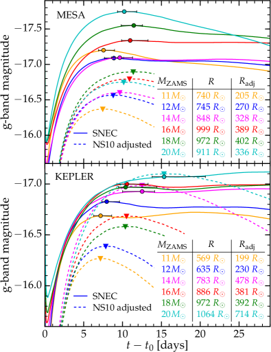
Figure 5.— The light curves in $g$-band for the MESA (top panel) and KEPLER (bottom panel) models from Figure 2 for $E_{\rm fin}=10^{51}\,{\rm erg}$. Solid lines show the output of SNEC, and colored circles indicate their local maxima. Dashed lines are obtained from Equations (29) and (31) of NS10 by varying the radius in order to reproduce the rise times of the numerical light curves while keeping the mass and the final energy fixed. Colored triangles indicate the maxima of the analytic light curves, and $R_{\rm adj}$ gives the radius obtained in this way (cf. González-Gaitán et al. 2015). The error bars show the time intervals during which the magnitude differs from the maximum by less than $0.01\,{\rm mag}$.

4. The rise times of SNe IIP

During the last several decades, numerical modeling of SN IIP bolometric light curves was focused on reproducing their gross properties, such as the length and the luminosity of the plateau (see Popov, 1993; Kasen & Woosley, 2009; Bersten et al., 2011). However, as was shown in the analytical works of NS10 and Goldfriend et al. (2014), the slopes of the light curves during the shock-cooling and plateau phases encode important information on the structure of the density profiles of the progenitor stars. Increasing abundance and quality of observational data has made it possible to conduct systematic studies of the early slopes for large sets of SN IIP light curves (Anderson et al., 2014; González-Gaitán et al., 2015). Modeling the slopes of the observed light curves and deducing the characteristics of the progenitor stars based on these slopes will be a very important task for future research.

In the current work, we instead focus on simply modeling the rise times of SNe IIP. Being more robust and easier to measure than the power law exponent of the bolometric light curve, the rise time can still give us important information on the progenitor characteristics. Our work is also motivated by a number of recent works considering large sets of early SN IIP light curves and focusing on their rise times (e.g., González-Gaitán et al., 2015; Rubin et al., 2016; Gall et al., 2015).

Figure 5 shows $g$-band light curves for a respresentative set of models from Figure 2, for a final energy $E_{\rm fin}=10^{51}\,{\rm erg}$. In our calculations, the SN emits as a blackbody at all times. Although the Rayleigh-Jeans part of the spectrum should not be strongly affected by this assumption during the shock cooling phase (Tominaga et al., 2011), this will be more directly addressed in future work (Shussman et al., 2016b, in preparation). The light curves generated by SNEC are plotted with solid lines. The colored circles indicate the local maxima of the light curves. Here we define the rise time, $t_{\rm rise}$, as the time between shock breakout and the local maximum of the color light curve in a given band. The error bars show the intervals of time during which the magnitude differs from the maximum by less than $0.01\,{\rm mag}$. Later in this paper (Figures 6 and 7), we take this criterion as a definition of the uncertainty with which the rise time can be measured. We choose $g$-band for the current study because in $u$-band the light curves are more sensitive to non-thermal effects like iron-group line blanketing (see Figure 8 of Kasen & Woosley, 2009), which are not properly taken into account in SNEC. Furthermore, $g$-band is a good match to many current and future optical surveys. In $r$-band, the light curves become very flat, which makes it difficult to robustly identify the maximum.

We note that in some of our calculations we find that the rise time depends on the duration of the thermal bomb. To investigate this dependence, we modeled the light curves of the KEPLER models for bomb durations of $0.1\,{\rm s}$, $10^{-2}\,{\rm s}$, $10^{-3}\,{\rm s}$, and $5\times 10^{-4}\,{\rm s}$. The vast majority of models show rise times independent of the bomb duration. The largest variations in $t_{\rm rise}$ ($\sim 4\,{\rm days}$) are seen for models with ZAMS masses in the range between $\sim 13\,M_{\odot}$ and $\sim 16\,M_{\odot}$ and at $E_{\rm fin}=2\times 10^{51}\,{\rm erg}$. These models have fully converged rise times only at $t_{\mathrm{bomb}}\leq 10^{-3}\,\mathrm{s}$. We believe that the observed dependence is due to the way the outer core structure in these models reacts to abrupt vs. to more gradual energy input. In first-principles core-collapse supernova simulations (e.g., Bruenn et al. 2016), the initial energy input by the expanding shock is abrupt, but most of the explosion energy builds up only gradually over $\sim$$1\,\mathrm{s}$. Since our thermal bomb approach does not allow us to fully realistically model the energy injection, we chose a thermal bomb duration of $10^{-3}\,\mathrm{s}$, which gives converged rise times for all our models.

For comparison with SNEC results, the dashed lines in Figure 5 show the light curves obtained from Equations (29) and (31) of NS10 for RSGs. For the values of mass and energy in these equations we use the ejecta mass $M_{\rm ej}$ and the final energy $E_{\rm fin}$ of each model. We choose the radius in these equations, $R_{\rm adj}$, in such a way that the maximum of the analytical light curve coincides in time with the maximum of the corresponding numerical SNEC light curve (the colored triangles indicate the maxima of the analytical light curves). By doing so we mimic the way in which the progenitor radii were derived from the rise times in González-Gaitán et al. (2015). One can see that the values of $R_{\rm adj}$ are on average a factor of $\sim 1.5-2.5$ smaller than the actual radii of the RSG models. Taking this factor into account would bring the results of González-Gaitán et al. (2015) in much better agreement with the observed radii of RSGs (see Levesque et al., 2005, 2006) and with the radii of the RSG models shown in Figure 1.

As an aside, we note that from Figure 5 it may seem that the numerical and analytical light curves have different breakout times (note the offset of the light curves at early times). This is explained by the fact that during the planar phase of post-explosion expansion (first $1-2$ days), the $g$-band flux of the NS10 model goes down and starts to rise once the spherical phase of the expansion begins (this is also seen in the right hand panel of Figure 1 of González-Gaitán et al., 2015).

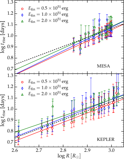
Figure 6.— The g-band rise time $t_{\rm rise}$ as a function of the progenitor radius $R$ for MESA (top panel) and KEPLER (bottom panel) models using three different values for the final explosion energy. Error bars denote the time over which the $g$-band absolute magnitude lies within $0.01\,{\rm mag}$ of the maximum (see Figure 5). Solid colored lines are linear fits to the same colored points in each panel. The black dashed line is the common fit for all models given by Equation (4).

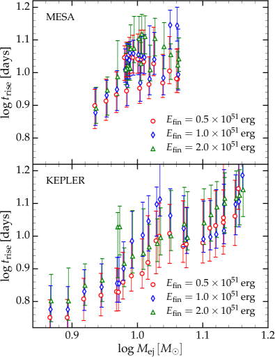
Figure 7.— The g-band rise time $t_{\rm rise}$ as a function of the ejecta mass $M_{\rm ej}$ for MESA (top panel) and KEPLER (bottom panel) models at the three considered values of the final explosion energy.

We next run a full collection of explosions using all stellar models and final energies of $0.5\times 10^{51}\,{\rm erg}$, $10^{51}\,{\rm erg}$, and $2\times 10^{51}\,{\rm erg}$. The main results of this set of calculations are summarized in Figures 6 and 7, where we plot g-band $t_{\rm rise}$ for all considered models as a function of $R$ and $M_{\rm ej}$, respectively. Figure 6 demonstrates that there is a strong correlation between the rise time and the radius of the progenitor. Furthermore, both the MESA and KEPLER models show similar dependences on $R$. On average, larger final energies have longer rise times, but this dependence is less strong. On the other hand, when we compare the rise time to the ejecta mass in Figure 7, the results are more mixed. The KEPLER models (bottom panel) show some correlation, but the spread is much larger than in the radius comparison. In addition, some of this dependence clearly comes from the strong correlation between mass and radius in the KEPLER models (Figure 1). The MESA models (top panel) show even less correlation with different masses sometimes having the same rise time.

In principle, one should be able to derive the dependence of the rise time on the radius and ejecta mass of the model in the form $\log t_{\rm rise}=a_{1}\log M_{\rm ej}+a_{2}\log R+a_{3}$ with constant coefficients $a_{1}$, $a_{2}$ and $a_{3}$. Unfortunately, correlations between radius and mass as shown in Figure 1 make it difficult to isolate these dependencies. As a consequence, the values of $t_{\rm rise}$ for our models form nearly a line in the three-dimensional space $(\log M_{\rm ej},\log R,\log t_{\rm rise})$, and we find that it is not conclusive to fit a surface of the form $\log t_{\rm rise}=a_{1}\log M_{\rm ej}+a_{2}\log R+a_{3}$. In the future, this dependence could possibly be inferred by fitting a much larger range of models with different masses and radii.

On the other hand, comparing the MESA models in the top panels of Figures 6 and 7 reveals that there is a much clearer mapping between radius and rise time than between ejecta mass and rise time. This is especially apparent in the mass dependence of the rise time in the MESA models (top panel of Figure 7), which shows that the same ejecta masses can have different rise times when the radius is different. This was generally expected from previous analytic work (NS10, Piro & Nakar 2013), but it is helpful how clearly it is seen here. Furthermore, Figure 6 shows that both the MESA and KEPLER models have similar relationships (both slope and normalization) between radius and rise time. Motivated by this, we find a linear fit for $\log t_{\rm rise}$ as a function of $\log R$. Colored lines in Figure 6 show the fits taken separately for each set of models and each value of the final energy. The black dashed line is the common fit in g-band for all models and all final (explosion) energies, which has the following numerical coefficients,

$$\log R\,[R_{\odot}]=1.225\log t_{\rm rise}\,[{\rm day}]+1.692\ .$$ (4)

From Figure 6 one can see that the slope of the radius dependence is fairly insensitive to the model type (KEPLER or MESA) and final energy. Equation (4) can be used as a tool to infer the radii of SN IIP progenitors from current and future transient surveys. This will be especially useful for analyzing large collections of events where it is impractical to do individual modeling.

An analogous relation to Equation (4) between the rise time in the optical part of the spectrum and the progenitor characteristics was obtained in Gall et al. (2015). From the analytical model of Arnett (1980, 1982), they found that the optical rise time scales as $t_{\rm opt-rise}\propto R^{1/2}T_{\rm peak}^{-2}$, while for the Rabinak & Waxman (2011) model, $t_{\rm opt-rise}\propto R^{0.55}T_{\rm peak}^{-2.2}E_{51}^{0.06}M_{\rm ej}^{-0.12}$, where $T_{\rm peak}$ is the effective temperature at the peak and $E_{51}$ is the final explosion energy in units of $10^{51}\,{\rm erg}$. In comparison, we find a somewhat stronger relation of $t_{\rm rise}\propto R^{0.816}$, although we do not include the temperature dependence. In the future, by running a large set of models with more diversity in their ejecta-mass–radius relations, we will be able to better study how $t_{\rm rise}$ depends on other factors besides radius.

Assuming that the rise times we find are representative of what is found in nature, we can also ask what should be expected for the rise times in a larger sample of events. Since the distribution of massive stars is understood in terms of an initial mass function (and not a radius function), we have to assume a mass-radius relation to explore this. In this case we use the KEPLER models and a final energy $E_{\rm fin}=10^{51}\,{\rm erg}$. Using Monte Carlo techniques, we generate a large sample of massive stars with ZAMS masses in the range between $8\,M_{\odot}$ and $20\,M_{\odot}$ (motivated by the masses approximately inferred by pre-explosion imaging of SNe IIP, Smartt et al. 2009) with a Salpeter initial mass function of

$$\frac{dN}{dM_{\rm ZAMS}}\propto M_{\rm ZAMS}^{-2.35}\ ,$$ (5)

and calculate their rise times. The median value of the derived set of rise times is $7.27$ days, which is similar to the observed median value of $7.5\pm 0.3$ days found by González-Gaitán et al. (2015). This implies a median radius of $559\,R_{\odot}$ for SNe IIP progenitors. This value is interesting for comparison to observational samples of massive stars (e.g., Levesque et al., 2005, 2006).

5. Conclusions and discussion

Using SNEC (Morozova et al., 2015), we have exploded a set of massive star models from both the KEPLER and MESA stellar evolution codes to study how the rise of the SN light curve depends on progenitor and explosion characteristics. We find that the strongest correlation is between the g-band rise time and the radius at the time of explosion, and provide a formula that relates these two properties in Equation (4). This can be used in future analyses of SNe IIP observations.

To better understand what properties of the progenitor are controlling the early light curve, we examined the envelopes of red supergiants obtained with both stellar evolution codes. We find that their convective envelopes do not extend all the way to the surface. In fact, all the considered models have regions close to their surface where the power-law exponent $n$ is smaller than $1.5$ and its value varies between different ZAMS masses. These regions are important for the early light curve, since the luminosity shell passes through them during the first $10-25$ days after shock breakout. Due to the shallow density profiles in these regions, the simple estimate $\hat{\tau}=c/\hat{v}$ for the optical depth at the luminosity shell is inadequate. This explains the differences we find with previous semi-analytic treatments of the early light curve.

The results obtained in this paper add to a long standing discussion about the progenitor radii of SNe IIP. Based on the results of their numerical models, Dessart et al. (2013) showed that the color properties of SNe IIP may be explained by small progenitor models ($\sim 500\,R_{\odot}$), while larger progenitors would produce light curves that remain too blue for too long. González-Gaitán et al. (2015) came to a similar conclusion based on a comparison of the observed rise times to analytical models of the shock-cooling phase. The radii they obtain are a factor of $\sim 2$ smaller than the observed radii of RSGs (see Levesque et al., 2005, 2006), and have the median value $\sim 350\,R_{\odot}$. Progenitor radii $\lesssim 500\,R_{\odot}$ are also suggested by the results of Shussman et al. (2016a) and Garnavich et al. (2016). At the same time, the works of Valenti et al. (2014) and Bose et al. (2015) for two SNe IIP deduce large radii (up to $\sim 800\,R_{\odot}$) for their progenitor stars. Rubin et al. (2016) find that the progenitor radii are weakly constrained by comparison to analytical shock-cooling models (at least based on $R$-band photometry alone). In this paper, we have shown that deriving the progenitor radius in the way done in González-Gaitán et al. (2015) may considerably underestimate it. On the other hand, exploding the MESA and KEPLER stellar evolution models without reducing their radii, we find a reasonable agreement with the median value of the observed $g$-band rise times from González-Gaitán et al. (2015).

One of the main strengths of our technique is that it does not require that the stellar models we use exactly replicate the progenitors that exist in nature. Instead, having a more diverse sample of models with different mass-radius relations gives us an increasingly better handle on how the early rise depends on the progenitor properties. Therefore, for future work it will be useful to explode an even larger set of stellar models. This would help better test the relation we find between rise time and radius, but also help us to better understand how sensitive the rise time is to the ejecta mass. In addition, one could explore whether $T_{\rm peak}$, the temperature at peak, is useful for tightening this relation, as has been found in previous semi-analytic work (see Gall et al., 2015). In this way, a fairly easy additional observable, namely the colors at peak, could be used to make these radius measurements more robust. This will be useful as a tool for future transient surveys, as well as for comparison with pre-explosion imaging of SNe and studies of massive stars that hope to connect these progenitors to the SNe they will eventually make.

References

- Anderson et al. (2014) Anderson, J. P., González-Gaitán, S., Hamuy, M., et al. 2014, ApJ, 786, 67
- Arnett (1980) Arnett, W. D. 1980, ApJ, 237, 541
- Arnett (1982) —. 1982, ApJ, 253, 785
- Bersten et al. (2011) Bersten, M. C., Benvenuto, O., & Hamuy, M. 2011, ApJ, 729, 61
- Bersten et al. (2012) Bersten, M. C., Benvenuto, O. G., Nomoto, K., et al. 2012, ApJ, 757, 31
- Bose et al. (2015) Bose, S., Valenti, S., Misra, K., et al. 2015, MNRAS, 450, 2373
- Bruenn et al. (2016) Bruenn, S. W., Lentz, E. J., Hix, W. R., et al. 2016, ApJ, 818, 123
- Chiavassa et al. (2009) Chiavassa, A., Plez, B., Josselin, E., & Freytag, B. 2009, A&A, 506, 1351
- Dessart et al. (2013) Dessart, L., Hillier, D. J., Waldman, R., & Livne, E. 2013, MNRAS, 433, 1745
- Eastman et al. (1994) Eastman, R. G., Woosley, S. E., Weaver, T. A., & Pinto, P. A. 1994, ApJ, 430, 300
- Fraser et al. (2012) Fraser, M., Maund, J. R., Smartt, S. J., et al. 2012, ApJ, 759, L13
- Gall et al. (2015) Gall, E. E. E., Polshaw, J., Kotak, R., et al. 2015, A&A, 582, A3
- Garnavich et al. (2016) Garnavich, P. M., Tucker, B. E., Rest, A., et al. 2016, ApJ, 820, 23
- Goldfriend et al. (2014) Goldfriend, T., Nakar, E., & Sari, R. 2014, submitted to ApJ; arXiv:1404.6313
- González-Gaitán et al. (2015) González-Gaitán, S., Tominaga, N., Molina, J., et al. 2015, MNRAS, 451, 2212
- Kasen (2010) Kasen, D. 2010, ApJ, 708, 1025
- Kasen & Woosley (2009) Kasen, D., & Woosley, S. E. 2009, ApJ, 703, 2205
- Levesque et al. (2005) Levesque, E. M., Massey, P., Olsen, K. A. G., et al. 2005, ApJ, 628, 973
- Levesque et al. (2006) —. 2006, ApJ, 645, 1102
- Li et al. (2006) Li, W., Van Dyk, S. D., Filippenko, A. V., et al. 2006, ApJ, 641, 1060
- Matzner & McKee (1999) Matzner, C. D., & McKee, C. F. 1999, ApJ, 510, 379
- Maund et al. (2013) Maund, J. R., Fraser, M., Smartt, S. J., et al. 2013, MNRAS, 431, L102
- Morozova et al. (2015) Morozova, V., Piro, A. L., Renzo, M., et al. 2015, ApJ, 814, 63
- Nakar & Piro (2014) Nakar, E., & Piro, A. L. 2014, ApJ, 788, 193
- Nakar & Sari (2010) Nakar, E., & Sari, R. 2010, ApJ, 725, 904
- Paxton et al. (2011) Paxton, B., Bildsten, L., Dotter, A., et al. 2011, ApJS, 192, 3
- Paxton et al. (2013) Paxton, B., Cantiello, M., Arras, P., et al. 2013, ApJS, 208, 4
- Paxton et al. (2015) Paxton, B., Marchant, P., Schwab, J., et al. 2015, ApJS, 220, 15
- Piro (2012) Piro, A. L. 2012, ApJ, 759, 83
- Piro (2015) —. 2015, ApJ, 808, L51
- Piro et al. (2010) Piro, A. L., Chang, P., & Weinberg, N. N. 2010, ApJ, 708, 598
- Piro & Nakar (2013) Piro, A. L., & Nakar, E. 2013, ApJ, 769, 67
- Popov (1993) Popov, D. V. 1993, ApJ, 414, 712
- Rabinak & Waxman (2011) Rabinak, I., & Waxman, E. 2011, ApJ, 728, 63
- Rubin et al. (2016) Rubin, A., Gal-Yam, A., De Cia, A., et al. 2016, ApJ, 820, 33
- Shussman et al. (2016a) Shussman, T., Nakar, E., Waldman, R., & Katz, B. 2016a, submitted to ApJ; arXiv:1602.02774
- Shussman et al. (2016b) Shussman, T., Waldman, R., & Nakar, E. 2016b, in preparation
- Smartt et al. (2009) Smartt, S. J., Eldridge, J. J., Crockett, R. M., & Maund, J. R. 2009, MNRAS, 395, 1409
- Sukhbold et al. (2016) Sukhbold, T., Ertl, T., Woosley, S. E., Brown, J. M., & Janka, H.-T. 2016, accepted for publication in ApJ; arXiv:1510.04643
- Sukhbold & Woosley (2014) Sukhbold, T., & Woosley, S. E. 2014, ApJ, 783, 10
- Tominaga et al. (2011) Tominaga, N., Morokuma, T., Blinnikov, S. I., et al. 2011, ApJS, 193, 20
- Valenti et al. (2014) Valenti, S., Sand, D., Pastorello, A., et al. 2014, MNRAS, 438, L101
- Van Dyk et al. (2012) Van Dyk, S. D., Cenko, S. B., Poznanski, D., et al. 2012, ApJ, 756, 131
- Weaver et al. (1978) Weaver, T. A., Zimmerman, G. B., & Woosley, S. E. 1978, ApJ, 225, 1021
- Woosley & Heger (2007) Woosley, S. E., & Heger, A. 2007, Phys. Rep., 442, 269
- Woosley & Heger (2015) —. 2015, ApJ, 810, 34
- Young (2004) Young, T. R. 2004, ApJ, 617, 1233