Construction and enumeration of circuits capable of guiding a miniature vehicle

Abstract.

In contrast to traditional toy tracks, a patented system allows the creation of a large number of tracks with a minimal number of pieces, and whose loops always close properly. These circuits strongly resemble traditional self-avoiding polygons (whose explicit enumeration has not yet been resolved for an arbitrary number of squares) yet there are numerous differences, notably the fact that the geometric constraints are different than those of self-avoiding polygons. We present the methodology allowing the construction and enumeration of all of the possible tracks containing a given number of pieces. For small numbers of pieces, several variants are proposed which allow the consideration or not of the fact that the obtained circuits are identical up to a given isometry. For greater numbers of pieces, only an estimation will be offered. In the latter case, a randomly construction of circuits is also given. We will give some routes for generalizations for similar problems.

1. Introduction

Children’s tracks have existed for a long time, and allow the transportation of small wooden trains, as well as cars or model trains. One may refer, for example, to the trademarks Brio ®, Scalextric ® or Jouef ®. Today there are tracks formed of a very large number of different pieces, i.e. larger than ten. This large number of pieces is interesting, as it allows the production of different circuits from the same set of pieces. On the other hand, due to this large number of different pieces, there are also numerous situations where it is not possible to simply connect the two extremities so as to close the circuit. In certain cases this is simply not possible. To overcome this inconvenience, one solution consists of including additional guide pieces, allowing the connection of the track’s extremities which were previously unable to connect. This therefore leads to an increase in the number of different pieces, and creates new situations where it is not possible to connect the two extremities of the track. Often, the circuits offered demonstrate some play, to a greater or lesser extent, which allows the creation of large circuits. This play, of a geometric origin, is taken into account in the pieces constituting these circuits. For example, the (mortise and tenon) connecting parts of Brio ® track pieces allow them to move very slightly with respect to each other (the “Vario system”; see http://www.woodenrailway.info/track/trackmath.html). Model train tracks can be slightly deformed in order to close the circuit. The accumulation of this play indeed allows the closure of the constructed circuit, however the play often renders it difficult to close the circuit and, if it does close, it is also possible that the resulting discontinuity derails the miniature vehicles which use these circuits. There also exist, on the opposite scale, circuits formed of very few different pieces. The number of closed circuits achievable with a given set of pieces is then very low. For example, there often exists only a single combination of the pieces of this set allowing the circuit to close.

The patented system aims to overcome these drawbacks by offering a circuit or a set of guiding pieces which

• allows the realization of a large number of closed circuits from the same set of pieces,

• uses a minimum of different guide pieces,

• guarantees that it is always possible to simply close the circuit.

The play between the pieces of this system will be strictly zero, in contrast with traditional systems, allowing a perfect fit of circuit loops. The manufacturing will nonetheless provide a very small play, allowing the pieces to be connected to each other by mortise and tenon joints. Typically, this system concerns the domain of train tracks for children, though it may equally concern that of circuits for small cars and the like.

The construction of the pieces of the circuits, which has led to a patent [, Bas13], is not the subject of this article, though it is briefly recalled in section 2. We note however that, from a pedagogical and didactic point of view, the construction of these circuits has been the subject of various presentations to different audiences, from the general public, to high school students, to a informal seminar for final-year undergraduates to doctoral students (see [Bas15a, Bas15]). These circuits employ various notions of geometry, spanning the curricula of middle and high school up to undergraduate studies (Pythagoras’ theorem, tangents, circles, parabolas, Bézier curves, radii of curvature, tessellation and enumerative combinatorics), which may be brought up in a distinguished way, and adapted to the relevant public. A collaboration is planned with Nicolas Pelay from the Plaisir Maths association (http://www.plaisir-maths.fr/), and we will try together to promote the game on it’s pedagogical and didactic aspect.

The initial motivation of the work presented here was a question asked by a manufacturer: << Is it possible to tally all of the circuits which can be realized from a given number of pieces? >> The objective of this article is to attempt to respond to this question. We will present in Section 3 the methodology allowing the construction and enumeration of all of the possible circuits containing a given number of pieces. For greater numbers of pieces, only an estimation will be offered (Section 4). In the latter case, a randomly construction of circuits is also given (Section 5). We will give some routes for generalizations in Section 6.

One may refer to the dedicated web page in French :

http://utbmjb.chez-alice.fr/recherche/brevet_rail/detail_brevet_rails.html

All of the algorithms presented in this article have been implemented computationally and have allowed the determination of the different circuits presented, as well as their to-scale depiction. Four executables (distributed for Windows only) and a documentation in French allowing the installation of graphical libraries, the creation of circuits in a manual or random manner, and the drawing of the circuits are available on the internet at the URLs:

http://utbmjb.chez-alice.fr/recherche/brevet_rail/MCRInstaller.exe

http://utbmjb.chez-alice.fr/recherche/brevet_rail/creecircuit.exe

http://utbmjb.chez-alice.fr/recherche/brevet_rail/creecircuitaleat.exe

http://utbmjb.chez-alice.fr/recherche/brevet_rail/dessinecircuit.exe

http://utbmjb.chez-alice.fr/recherche/brevet_rail/mode_emploi_rail_demo.pdf

A catalogue has been created in a totally automatic manner (apart from the few manually determined circuits), grouping together the different methods presented here, and is available at the following URL:

http://utbmjb.chez-alice.fr/recherche/brevet_rail/catalogue.pdf

One can also look up all of the first $1102$ feasible circuits (the total number of pieces used varies from $4$ to $11$ and the maximal number of each kind of piece is $4$) at

http://utbmjb.chez-alice.fr/recherche/brevet_rail/catalogue_exhaustif_11rails.pdf

2. Principles of the patented system

2.1. Construction of the basic curves

The principle of this system is to define a path $\Gamma$ in $\mathbb{R}^{2}$, and of class ${\mathcal{C}}^{1}$, which ensures continuity between two successive pieces of the circuit, as well as their good fit. Let $N$ be any non-zero natural number. Two fundamental ideas are used:

• We consider a set of squares ${\mathcal{C}}_{i}$, $1\leq i\leq N$ each belonging to a square tiling of the plane. The side of each square is defined by

  $$L_{0}=1.$$ (1)

  We will then assume, without loss of generality, that the coordinates of the centers of the squares ${\mathcal{C}}_{i}$ are integers. Each square contains a part of the path $\Gamma$, and the intersection of a square ${\mathcal{C}}_{i}$ with $\Gamma$ is denoted $\Gamma_{i}$.

• For each of the squares ${\mathcal{C}}_{i}$, the curve $\Gamma_{i}$ must satisfy the following constraints:

  • it is contained within the square ${\mathcal{C}}_{i}$,

  • it begins on one vertex of the square, or in the middle of one side of the square, at a point $A_{i}$, and ends on another vertex of the square, or in the middle of another side, at a point $B_{i}$,

  • it is tangent at $A_{i}$ and at $B_{i}$ to the straight lines connecting respectively the center of the square to the points $A_{i}$ and $B_{i}$.

Thus, the path $\Gamma$ will be defined as the union of the curves ${(\Gamma_{i})}_{1\leq i\leq N}$. For $1\leq i\leq N-1$, each of the squares ${\mathcal{C}}_{i}$ must have a unique vertex or side in common with the neighboring square ${\mathcal{C}}_{i+1}$. If $i=N$, then the same rule applies for the squares ${\mathcal{C}}_{1}$ and ${\mathcal{C}}_{N}$. One may hence define the path $\Gamma$, from the centers ${(c_{i})}_{1\leq i\leq N}$ of the squares ${\mathcal{C}}_{i}$ with integer coordinates. This problem is therefore very similar to the research into self-avoiding walks, described in [Sla11, MS93], in the planar case, and also in the particular case where the origin and the end are identical, i.e. the case of the self-avoiding polygons, described in [Sla11, Jen03, JG99, Gut12a, Gut12, CJ12]. Five essential differences distinguish the game’s circuits from self-avoiding polygons. On the one hand, in [Sla11, Jen03, JG99, Gut12a, Gut12, CJ12], while the squares must necessarily be distinct, the Easyloop system allows two non-successive squares to be confounded; we will return to this point in Section 3.4. On the other hand, in [Sla11, Jen03], two successive squares may only have one side in common, in contrast with the Easyloop system. Furthermore, some additional constraints due to the number of available pieces are to be considered in the Easyloop system.It will only be necessary to keep circuits which are different up to an isometry. See section 3.3. Finally, the number of pieces used in self-avoiding polygons is necessarily even; in the case of an odd number of pieces, no polygon exists, which is not the case for the circuits.

Remark 2.1.

In [Jen04a], a generalization of self-avoiding walks is mentioned. These evolve in a tiling of the plane formed of isosceles right triangles (see Figure 1 of this reference), each corresponding to half of a square. Our circuits are closer to this type of self-avoiding walk since, here, the possibility that two neighboring squares have a common vertex is taken into account. In the same reference, the Kagomé lattice is also mentioned, corresponding to an octagonal tile and a square tile (see Figure 1 of the reference). There again, more degrees of freedom are offered, but the proposed geometry is not exactly those of our circuits.

It now remains to define the geometry of each of the curves $\Gamma_{i}$. Let us fix $i\in\{1,...,N\}$. We call ${\mathcal{H}}_{i}$, the set of eight points formed by the four middles and the four vertices of the square ${\mathcal{C}}_{i}$. To have a high number of circuits, we seek all of the possible curves corresponding to all of the possible choices of pairs of distinct points $A_{i}$ and $B_{i}$ in ${\mathcal{H}}_{i}$, which represents, a priori, $C^{2}_{8}=28$ cases. However, the square possesses a group of isometries $\mathcal{S}$ leaving it invariant, of cardinal 8, which reduces the number of possible curves to 6. We define 6 types of curve in the following way:

• a first type, grouping together only the curves for which the points $A_{i}$ and $B_{i}$ are the middles of two opposite sides of the square,

• a second type, grouping together only the curves for which the points $A_{i}$ and $B_{i}$ are the middles of two adjacent sides of the square,

• a third type, grouping together only the curves for which the points $A_{i}$ and $B_{i}$ are two diagonally opposite vertices of the square,

• a fourth type, grouping together only the curves for which the points $A_{i}$ and $B_{i}$ are two immediately consecutive vertices of the square,

• a fifth type, grouping together only the curves for which the points $A_{i}$ and $B_{i}$ are the middle of one side and a vertex of the opposite side of the square,

• a sixth type, grouping together only the curves for which the points $A_{i}$ and $B_{i}$ are the middle of one side and a vertex of the same side of the square.

Such constraints still do not totally define the curves, but we now seek them in the set of line segments or circular arcs, as in the world of the toy. In Figure 1, the six types of curves are presented. The first and third types contain only line segments of respective lengths $1$ and $\sqrt{2}$ (Figures 1(a) and 1(c)). The second and fourth types contain only quarter-circles, with respective radii $1/2$ and $\sqrt{2}/2$ (Figures 1(b) and 1(d)). Finally, for the last two types, no circular arcs exist. We therefore seek a solution, for example, in the form of a parabola defined by two points $A_{i}$ and $B_{i}$ and the two associated tangents. On may either determine the unique parabola thus defined, or equivalently, determine the unique Bézier curve of order two, which is then defined by the following control points: the point $A_{i}$, the center of the square $c_{i}$ and the point $B_{i}$ (Figures 1(e) and 1(f)). One may refer to [FHK02, HM13, Per, LH97, Bas15].

(a) Form 1

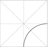
(b) Form 2

(c) Form 3

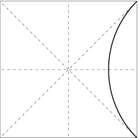
(d) Form 4

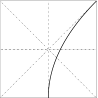
(e) Form 5

(f) Form 5’

Figure 1. The six basic forms.

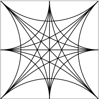
(a) with 5 basic pieces

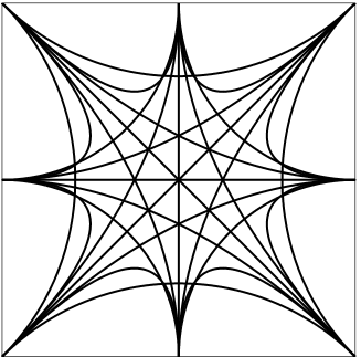
(b) with 6 basic pieces

Figure 2. The set of possible paths.

Acting on the 6 curves in Figure 1 with the group of 8 isometries $\mathcal{S}$, one indeed obtains the 28 possible curves of Figure 2(b). The sixth type in Figure 1(f) will be eliminated in the following, since the corresponding piece has a radius of curvature which is too small for the miniature vehicles to be able to ride there (see section 2.2), which reduces the number of possible paths to 20 (see Figure 2(a)). In this case, the rule << every curve linking any two distinct points in ${\mathcal{H}}_{i}$ >> is to be replaced by << every curve linking any two distinct non-neighboring points in ${\mathcal{H}}_{i}$ >>, which, as we will see in the following, nevertheless offers a large number of circuits.

The curve $\Gamma$ is of class ${\mathcal{C}}^{1}$; indeed, each of the curves $\Gamma_{i}$ is of class ${\mathcal{C}}^{\infty}$. Furthermore, the union of all of these curves will be of class ${\mathcal{C}}^{1}$. By construction, indeed, at the connecting points, which can only be vertices or middles of the sides of squares, the curves are continuous (since they pass by the same start and end points) and have a continuous derivative, since the tangents coincide.

The curves $\Gamma$ obtained are of class ${\mathcal{C}}^{1}$, but not of class ${\mathcal{C}}^{2}$, due to the discontinuity of the radius of curvature, in contrast with real rail and road networks. We note however that this discontinuity is also present in the existing traditional systems, constituted of straight-line and circular pieces of different radii of curvature. On a mechanical level, this generates, for the miniature vehicle which takes the circuit, a discontinuity of the normal acceleration (at constant velocity) and of the steering angle of the wheels. These constraints, significant for real vehicles, directly affect the comfort of the passenger and the wear induced on the mechanical parts, but are not taken into account in the domain of games. Indeed, the masses and the velocities of the vehicles are very low, and therefore the shocks due to the discontinuity of the normal acceleration are negligible. Moreover, the notion of the comfort of the passenger has no meaning here. Finally, the wheels of the vehicles may be subjected to a discontinuity of the steering angle since they exhibit a slight play with respect to the chassis.

2.2. Construction of the pieces

Once the path $\Gamma$ has been constructed, it remains to define the different types of tracks constituting the circuit. Each of the types of track will be defined from one of the five types of curves defined above.

• These curves constitute the midline of each of the types of piece.

• The wheel passages are defined as two curves at a constant distance from this middle curve, i.e: each point from one of these two curves is found on a straight line perpendicular to the tangent of the midline at constant distance from the middle curve. The edges of the tracks are defined in the same way.

• The cross section of the piece is defined in a conventional way.

• Note that in [], we specified that the half-width $e/2$ of the rail must be less than the radius of curvature of the midline in order to avoid that, at the considered point, the curve constructed at equal distance from the midline does not feature a stationary point with a change in the direction of the unit tangent vector. For the parabola in Figure 1(e), the minimal radius is $R_{\min}=1$, while for the parabola in Figure 1(f), the minimal radius is $R_{\min}=\frac{\sqrt{5}}{25}$. Thus, if we consider the curves in Figures1(a) to 1(e), the minimal radius of curvature is then

  $$R_{\min}=\frac{1}{2},$$

  whereas if we consider the curves in Figures 1(a) to 1(f), the minimal radius of curvature is then

  $$R_{\min}=\frac{\sqrt{5}}{25}.$$

  In the first case, the width $e$ of the rail is therefore strictly less than $e_{0}$, given by

  $$e_{0}=1,$$ (2)

  while in the second case, $e_{0}$ is given by

  $$e_{0}=\frac{2\,\sqrt{5}}{25}\approx 0.17889.$$ (3)

  The choice of a standard cross-section, compatible with Brio®-type vehicles, corresponds to

  $$e=0.18349.$$ (4)

  Thus, for the curves in Figures 1(a) to 1(e), this choice of width allows us to have no stationary points. On the other hand, for the curves in Figures 1(a) to 1(f), this choice of width presents a stationary point, as exhibited by pieces 7 and 8 in Figure 3.

• Finally, the connectors are mortise and tenon joints, designed such that each track possesses one mortise and one tenon.

Piece-types 1 to 4 are symmetric: they possess a symmetry plane perpendicular to the middle curve, and since the cross section is itself symmetric, it is therefore sufficient to construct a single type of piece for each of these four types. On the other hand, the type 5 piece isn’t symmetric, and the two extremities therefore do not play the same role. In order to realize the circuit, it was therefore necessary to construct two different pieces where the male and female connectors are inverted.

The extremities of the pieces may be either middles of side or vertices, and it was necessary to mark on the rails the extremities corresponding to vertices, which was done using a yellow dot. This dot also appears on all of the track designs which will be presented in this document. The child which plays at assembling the pieces will therefore have this single rule to obey: << only put pieces together if the two extremities of two contiguous pieces have the same nature (simultaneous absence or presence of dots) >>. This rule is the only one to be obeyed in order to be able to make circuits which loop properly!

Finally some prototypes were manufactured. The theoretical squares shown with side of length given by (1) have all been multiplied by a reference length given by

$$L=21.8\,\text{cm},$$ (5)

which is equal to the side of the basic square constituting the real tiling.

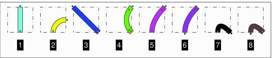
Figure 3. The numbering of the parts.

The pieces are henceforth numbered as indicated in Figure 3.

Recall that pieces 7 and 8  present in theory in the circuit, were not produced in practice, since they are too curved. The calculations presented in the following can certainly take into account these two types of piece, but for simplicity we will henceforth assume that only the first six types of piece are used. However, the programs and algorithms described can also provide for the presence of these two pieces.

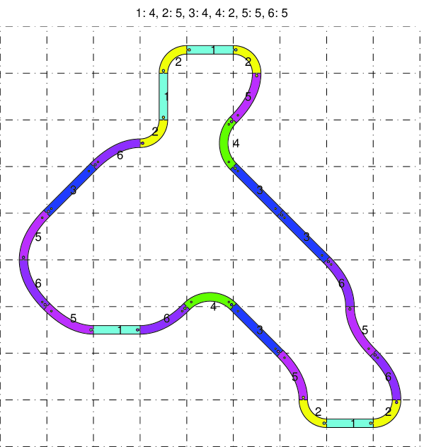
Figure 4. An example track design.

We give an actually manufactured circuit as an example in Figure 4.

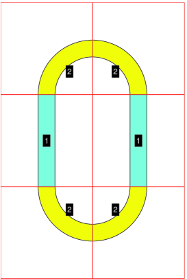
(a) Circuit map representation

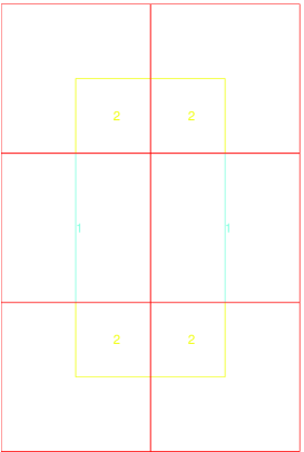
(b) Self-avoiding polygon

Figure 5. An example circuit.

In Figure 5, we have represented a track design, seen as a game map (Figure 5(a)) or as a self-avoiding polygon (Figure 5(b)), obtained by by joining the centers $c_{i}$. In this case, the circuit is a self-avoiding polygon in the classical sense of the term.

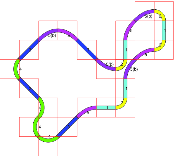
(a) Circuit map representation

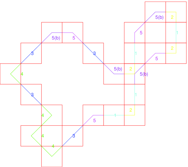
(b) Self-avoiding polygon

Figure 6. An example circuit.

In Figure 6, we have represented a track design seen as a game map (Figure 6(a)) or as a self-avoiding polygon (Figure 6(b)). The latter figure highlights the essential differences which exist between our self-avoiding polygons and those in the literature; ours allow successive squares to have a vertex in common, and two different squares may be occupied by two different trajectory parts.

3. Construction and enumeration of the circuits

3.1. Posing the problem

Recall the question which is of interest to the manufacturer: << Is it possible to tally all of the circuits which can be realized from a given number of pieces? >> For $1\leq j\leq 6$, we denote by $N_{j}\in\mathbb{N}\cup\{+\infty\}$ the number of pieces 1 to 6 available, and by $N$ the total number of pieces used, and we seek all of the circuits which close containing exactly $N$ pieces in all, and such that, for each type of piece, the number of pieces used in less than $N_{j}$. We necessarily have

$$N\leq\sum_{j=1}^{6}N_{j}.$$ (6)

The case $N_{j}=+\infty$ corresponds to the case where the type of pieces concerned is not a priori limited. However, the number of pieces of this type is necessarily less than $N$.

A circuit is totally determined by the $N$ centers ${(c_{i})}_{1\leq i\leq N}$ of the squares. These centers being given, it is therefore possible to determine, by taking the middles of two successive centers, the coordinates of the points $A_{i}$ and $B_{i}$ for each square, which correspond to the start and end of the curve $\Gamma_{i}$ in square ${\mathcal{C}}_{i}$. Consideration of the mortises and tenons orients the circuit, and it is necessary to consider this orientation for pieces 5 and 6. Let us choose an orientation of the mortises and tenons (which amounts to orienting the circuit) in the following way: if the circuit is traversed in increasing order of the square indices, $1,2,\ldots,$ then in each square, the first extremity of the piece corresponds to the female connector and the second corresponds to the male one. We denote by $p_{i}\in\{1,...,6\}$, the type of piece concerned in square ${\mathcal{C}}_{i}$. We will write respectively $A_{i}$ and $B_{i}$ (elements of ${\mathcal{H}}_{i}$), for the start of the curve $\Gamma_{i}$, corresponding to the female connector, and the end of the curve $\Gamma_{i}$, corresponding to the male connector. The number $p_{i}$ therefore depends only on the points $A_{i}$ and $B_{i}$. For example, if these two points are two successive vertices, the piece is of type 4.

Another way to see this is to notice that each piece is totally determined by the relative position of the square containing the previous piece and the one containing the following piece, as well as the nature of the points $A_{i}$ and $B_{i}$ (that is, being a vertex or middle). To this end, for $i\in\{2,...,N-1\}$, we consider the angle

$$\alpha_{i}=\widehat{\left(\overrightarrow{c_{i-1}c_{i}},\overrightarrow{c_{i}c_{i+1}}\right)}\in[0,2\pi[.$$ (7)

Figure 7. Each piece is defined by the two squares delimiting it and the square to which it belongs.

See Figure 7. If we let

$$\forall i\in\{2,...,N-1\},\quad\alpha_{i}=\frac{k_{i}\pi}{4},$$ (8)

then the sole possible values of $k_{i}$ describe the set $\{0,1,2,6,7\}.$

$A_{i}$	$B_{i}$	$k_{i}$	type of piece
middle	middle	$0$	1
middle	middle	$2$ or $6$	2
vertex	vertex	$0$	3
vertex	vertex	$2$ or $6$	4
middle	vertex	$1$ or $7$	5
vertex	middle	$1$ or $7$	6

Table 1. Piece numbers $p_{i}$ as a function of $A_{i}$, $B_{i}$ and $k_{i}$

The relations between these elements are given in Table 1. In Figure 7, the example shows the case of a piece corresponding to $k_{i}=1$, that is, of type 6.

Remark 3.1.

In the case where $k_{i}\not=0$, the value of $k_{i}$ allows the determination of the turning direction of the piece in question (right or left). For $k_{i}=1$ or $k_{i}=2$, the piece turns towards the left, and for $k_{i}=6$ or $k_{i}=7$, it turns towards the right. One may therefore also associate a sign to the numbers of the curved pieces. Only the absolute value is important for counting of the different types of piece, but we will see later that it may be necessary to keep this sign in order to orient the direction in which this piece turns.

3.2. Description of all circuits

Firstly, we describe the search for all circuits with $N$ pieces for which the center of the first piece is arbitrarily equal to the origin, and center of the last is given by $(x,y)\in\mathbb{Z}^{2}$.

The second square, which is necessarily neighboring the origin, may be therefore chosen among 8 possible squares. For each of these choices, one may choose freely the values of $k_{i}$, $2\leq i\leq N-1$ from $\{0,1,2,6,7\},$ which fixes the values of $c_{i}$, $1\leq i\leq N$, as well as the values of the angles $\alpha_{i}$, $2\leq i\leq N-1$. We are given, moreover, the first point $A_{1}$ of the first curve (in ${\mathcal{H}}_{1}$) and the last point $B_{N}$ of the last curve (in ${\mathcal{H}}_{N}$). The point $B_{2}$ is known; from this we deduce the number of piece $p_{1}$. Likewise, $p_{N}$ is known. For all $i$, $2\leq i\leq N-1$, the natures of all of the points $A_{i}$ and $B_{i}$ and the value of $k_{i}$ are known, from which we deduce the value of $p_{i}$ using Table 1. Of all of the circuits thus defined, we will keep only those corresponding to $c_{N}=(x,y)$.

Thus, by varying a certain number of independent parameters, we are capable of enumerating all of the circuits, in a geometric (the determination of the $c_{i}$) and constitutive (determination of the $p_{i}$) way, going from the origin to a given point.

If one now seeks all of the circuits which form a loop, one will similarly consider the center of the first square to be arbitrarily equal to the origin. The last square $c_{N}$ can only be one of the 8 neighbors of the first one. By symmetry and rotation, one may simply choose $c_{N}\in\{(1,0),(1,1)\}$. For each choice of $c_{N}$, we apply that which we have seen above to determine all of the circuits going from the origin to $c_{N}$. In this case, the vertices $A_{1}$ and $B_{N}$ are necessarily known and equal, since they will necessarily be the vertex or the common middle of the first and last square. Note that one could also set, in a similar manner to (7) and (8),

$$\alpha_{1}=\widehat{\left(\overrightarrow{c_{N}c_{1}},\overrightarrow{c_{1}c_{2}}\right)}\in[0,2\pi[,$$ (9a)

$$\alpha_{N}=\widehat{\left(\overrightarrow{c_{N-1}c_{N}},\overrightarrow{c_{N}c_{1}}\right)}\in[0,2\pi[,$$ (9b)

and

$$\forall i\in\{1,N\},\quad\alpha_{i}=\frac{k_{i}\pi}{4}.$$ (10)

We will keep only the circuits such that $k_{1}$ and $k_{N}$ belong to the set $\{0,1,2,6,7\}.$ We hence deduce the values of the $N$ integers ${(p_{i})}_{1\leq i\leq N}$. Finally, of all of these circuits, we will keep only those for which the total number of each piece of each type is less than $N_{j}$.

This method, based on a parameter sweep, obtained as the Cartesian product of finite sets, is very costly in time, and is quickly limited for values of $N$ which are too large (we will return to this point in Section 3.6). In [Jen04, Sla11, Jen03, JG99, Gut12a, Gut12, CJ12], there exist some much more subtle and parallelizable techniques for the enumeration of all self-avoiding or polygons walks. However, we have already pointed out in the introduction the essential differences between our circuits and self-avoiding walks or polygons, which may render the use of the methods from [Jen04] ineffective here. Furthermore, the geometric trajectories of the circuits need to be determined in order to satisfy the constraint concerning the $N_{j}$. These circuits will also need to undergo eliminations to take into account the repetition of isometric circuits (see Section 3.3), as well as the satisfaction of a local constraint, which is not that of self-avoiding walks or polygons (see Section 3.4). Finally, we consider it important, in addition to counting all the circuits, to present them all, for small values of $N$ at least.

The disadvantage of this method is that it goes first through the determination of all possible circuits, which represents a very large number of circuits, and then keeps only those which form a loop. Another method will be to determine all of the looping geometric paths, either by Cartesian product, or in a recursive and parallel way. From all of these paths, one retains only those which correspond to a circuit. This method seems to be as long as the one shown above, and equally presents the disadvantage of having to determine a large number of elements, only to keep but a portion.

3.3. Consideration of the isometries

Let us begin by studying a simple example. We will choose a small value of $N$ without regard for the constraints imposed by $N_{j}$.

Example 3.2.

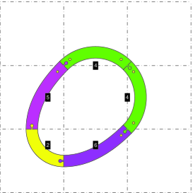
(a)

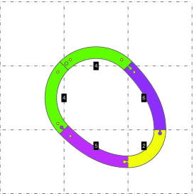
(b)

(c)

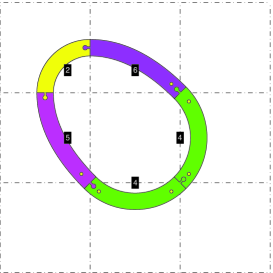
(d)

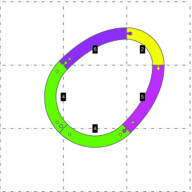
(e)

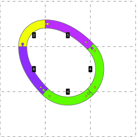
(f)

(g)

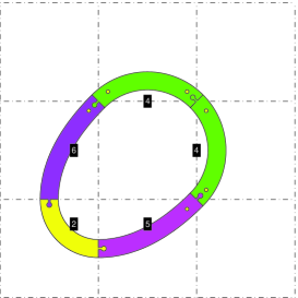
(h)

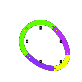
(i)

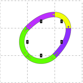
(j)

Figure 8. All of the 10 circuits kept from the set of 2000 possible circuits.

If we plot all the feasible circuits with $N=5$ pieces and $N_{j}=+\infty$, we obtain the $10$ circuits in Figure 8. In this figure, one can in fact see two different circuits repeating several times. In each of the two sets of circuits, one finds the same circuit up to a direct isometry. Two circuits are isometric (this isometry being direct) if and only if they both possess the same signed number of pieces (see Remark 3.1), up to cyclic permutations and up to direction of travel. We note that the total number of circuits examined equals $2000$.

(a)

(b)

Figure 9. All of the 2 circuits kept from the set of 2000 possible circuits.

If we keep only those which are different, up to a direct isometry, we obtain the $2$ circuits in Figure 9. In this figure, one notices that the first circuit is the image of the second under an indirect isometry. The numbers of the pieces are identical, up to cyclic permutations and up to direction of travel. Moreover, to take this indirect isometry into account, it is necessary to replace the signed numbers of curved pieces with their opposites.

Figure 10. The sole circuit kept from the set of 2000 possible circuits.

If we keep only those which are different up to an isometry, we obtain the unique circuit in Figure 10.

More generally, we draw all the circuits obtained for $N$ and $N_{j}$ given .

A consideration of the direct isometries will result in the comparison of all of the obtained circuits. If two among them possess the same signed numbers of pieces, up to cyclic permutations, then one of the two will be eliminated.

Secondly, a consideration of the indirect isometries will be performed. Similarly, if two circuits possess the same signed numbers of pieces, but which are opposite (for the curved pieces), up to cyclic permutations, then one of the two will be eliminated. To take all of the indirect isometries into account, it will also be necessary to eliminate the circuits by also comparing the indices with permutations of the type $N$, $N-1$, …, 2, 1, which amounts to considering the traversal of the circuit in the opposite direction. In this case, one will replace the signed number of pieces $\pm 5$ by $\mp 6$ and vice-versa. The two pieces 5 and 6 are in effect identical; only the orientation changes. This elimination will be legitimate if the number of available pieces of types 5 and 6 are identical, , which will always be true in the following (see remark 3.3).

Remark 3.3.

In the case of traditional self-avoiding polygons, the number of squares is necessarily even, which is no longer true here. Nonetheless, we can say that, in every circuit, the numbers of pieces of types 5 and 6 are equal. Indeed, note that, from Table 1,

• the pieces of type 1, 2, 3 and 4  connect together two points of the same nature (middles of sides or vertices of squares);

• the pieces of type 5 connect a middle to a vertex (in this order);

• the pieces of type 6 connect a vertex to a middle (in this order);

A circuit departs from a point and returns to the same point. All of the points corresponding to the extremities of the pieces used in the circuit are either vertices or middles. It follows that that there are as many pieces connecting a middle to a vertex (in this order) as pieces connecting a vertex to a middle (in this order). Otherwise, the point of departure would not be of the same nature as the point of arrival.

Remark 3.4.

Note that, in the enumeration of traditional self-avoiding polygons, only translations are taken into account in the isometries. Our enumeration problem is therefore quite different to the one in the literature. In the case where both notions coincide, this implies that the configurations that one will obtain will be a priori less numerous than those in the literature.

3.4. Consideration of local constructibility constraints

In the research into self-avoiding walks and polygons, a very important additional local constraint is considered: the squares must be pairwise distinct. Here, this constraint isn’t imposed, since only the fact of being able to produce circuits which are constructible with the real pieces counts. These constraints are not exhibited by Example 3.2, since the small number of pieces considered does not provide unconstructible circuits, but these constraints come up in larger circuits, exemplified below.

First of all, it is necessary that, aside from each of the pairs of contiguous pieces, which therefore have a unique extremity in common, none of the pieces has an extremity in common with other pieces which aren’t contiguous. If this extremity is a vertex, this criterion is easy to write, and is not detailed here. If this extremity is a middle, and if two non-contiguous pieces have this extremity in common, they necessarily belong to the same square, which is the case that we now study.

Two pieces may belong to the same square on the condition that they are disjoint (or have tangent edges).

(a) Case where the two midlines are necessarily secant: $K_{a}=\{2\}$, $K_{b}=\{0,4,5,6,7\}$

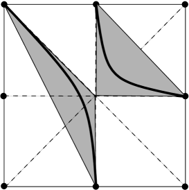
(b) Case where the two midlines are necessarily disjoint

Figure 11. Two pieces within a single square.

We therefore take two pieces in the same square ${\mathcal{C}}_{i}$, and we wish to verify that they are disjoint. Several cases present themselves:

1. They have at least one extremity in common. In this case, they are not disjoint.

2. Their extremities are pairwise distinct.

   1. We denote by $P_{1}=A_{i}$ and $P_{2}=B_{i}$ (respectively $P^{\prime}_{1}$ and $P^{\prime}_{2}$) the extremities of the first (respectively second) piece. The two points $P_{1}$ and $P_{2}$ belong to the border $\partial{\mathcal{C}}_{i}$ of the square. They therefore define two connected components (for the induced topology) denoted ${\mathcal{P}}_{a}$ and ${\mathcal{P}}_{b}$. If

      $$\text{($P^{\prime}_{1}\in{\mathcal{P}}_{a}$ and $P^{\prime}_{2}\in{\mathcal{P}}_{b}$) or ($P^{\prime}_{2}\in{\mathcal{P}}_{a}$ and $P^{\prime}_{1}\in{\mathcal{P}}_{b}$)},$$ (11)

      then the two vertices of the second piece are on both sides of the midline of the first piece, and by continuity of the midlines, they have a point in common and, necessarily, in this case, the two pieces are not disjoint. Conversely, if (11) does not hold, one can show that the midlines are necessarily disjoint (see case 2b).

      Let us clarify this. We describe the location of the extremities $P_{1}$ and $P_{2}$ of the first piece by two integers, $\kappa_{1}$ and $\kappa_{2}$, in $\{0,...,7\}$ in the following way: if $\vec{I}$ designates the first vector of the chosen orthonormal basis, and $c_{i}$ is the center of the square, then

      $$\widehat{\left(\vec{I},\overrightarrow{c_{i}P_{1}}\right)}=\frac{\kappa_{1}\pi}{4},\quad\widehat{\left(\vec{I},\overrightarrow{c_{i}P_{2}}\right)}=\frac{\kappa_{2}\pi}{4}.$$

      We similarly define $\kappa^{\prime}_{1}$ and $\kappa^{\prime}_{2}$ for the second piece. The set $\{0,...,7\}$ can be partitioned in the following way: $\{0,...,7\}=K_{a}\cup K_{b}\cup\{\kappa_{1}\}\cup\{\kappa_{2}\}$, such that all of the vertices corresponding to the indices of $K_{a}$ (respectively $K_{b}$) are consecutive in the square. Property (11) is equivalent to

      ($$\kappa^{\prime}_{1}\in K_{a} \kappa^{\prime}_{2}\in K_{b} \kappa^{\prime}_{2}\in K_{a} \kappa^{\prime}_{1}\in K_{b}$$ and ) or ( and ). (12)

      If this holds, the two pieces are not disjoint. See, for example, Figures 11(a) and 12(a), which illustrate this case.

   2. Let us now assume that (12) does not hold. In this case, $\kappa^{\prime}_{1}$ and $\kappa^{\prime}_{2}$ both belong to either $K_{a}$ or to $K_{b}$. If none of the pieces is straight, the cardinality of $K_{a}$ and $K_{b}$ is necessarily in $\{1,2\}$ or in $\{4,5\}$. Thus, $\kappa^{\prime}_{1}$ and $\kappa^{\prime}_{2}$ cannot belong to the smaller set, and we are necessarily in the case where the set of vertices contained between the two extremities of the first piece and the set of vertices contained between the two extremities of the second piece are disjoint. See for example Figure 11(b), which illustrates this case. A Bézier curve is necessarily included in the control polygon $A_{i}c_{i}B_{i}$. It is the same for the midlines of the circular pieces. Thus, in this case, each of the middle curves is included in two triangles which only have the center $c_{i}$ of the square in common, through which none of the midlines pass (since the straight midlines are not considered). This reasoning is still valid if one of the midlines is straight. In short, in this case, the midlines of the two pieces are disjoint.

It thus follows that, if the two pieces under consideration are coincident, we are in case 1. Otherwise we are either in case 1 or 2a, in which the pieces are not disjoint. Finally, if we are in the last case, 2b, the midlines of the two pieces are disjoint. In this case, if we write ${{\Gamma}}_{i}$ and ${{\Gamma}}^{\prime}_{i}$ for the two curves (which are in the same square), one may consider

$$\delta=\sqrt{\inf_{(M,M^{\prime})\in{{\Gamma}}_{i}\times\in{{\Gamma}}^{\prime}_{i}}d^{2}(M,M^{\prime})},$$ (13)

where $d(M,M^{\prime})$ is the Euclidean distance between the points $M$ and $M^{\prime}$. The pair $(M,M^{\prime})$ describes a compact subset of $\mathbb{R}^{2}$ and $d$ is continuous. This lower bound exists and is necessarily attained at a pair of points $(M_{0},M^{\prime}_{0})$ of ${{\Gamma}}_{i}\times{{\Gamma}}^{\prime}_{i}$. Since the two curves ${{\Gamma}}_{i}$ and ${{\Gamma}}^{\prime}_{i}$ are disjoint, the number $\delta$ is necessarily strictly positive. In addition, one can show that for every pair of curves ${{\Gamma}}_{i}\times{{\Gamma}}^{\prime}_{i}$ which fall into in this case, the real number $\delta$ is necessarily attained at a pair of points which cannot be at the edge of the square. In this case, since $(M,M^{\prime})\mapsto d^{2}(M,M^{\prime})$ is a differentiable function, its differential is zero there, which results in the perpendicularity of the straight line $(M_{0}M^{\prime}_{0})$ to the tangent to the curve ${{\Gamma}}_{i}$ (respectively ${{\Gamma}}^{\prime}_{i}$) at the point $M_{0}$ (respectively $M^{\prime}_{0}$).

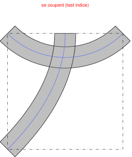
(a) Case where the two midlines are necessarily secant

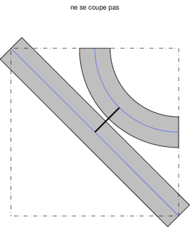
(b) Configuration where the distance between the two midlines is the smallest

Figure 12. Two pieces within the same square.

Computationally, all of these properties have been verified by conducting a sweep of all the possible pairs of curves ${{\Gamma}}_{i}\times{{\Gamma}}^{\prime}_{i}$, which represents $1600$ cases to study. We have determined the pair of curves which correspond to the smallest possible distance $\delta$, given by (in the case of a square of unit length):

$$\delta_{\min}=0.20711,$$ (14)

which corresponds to the configuration in Figure 12(b). This expression equals

$$\delta_{\min}=\frac{1}{2}\left(\sqrt{2}-1\right).$$ (15)

By construction of the edges, and by the perpendicularity properties seen above, at a constant distance equal to the half-width $e/2$ of the piece, two pieces will be disjoint if and only if

$$\delta_{\min}\geq e.$$ (16)

The case $\delta_{\min}=e$ corresponds to the case where the edges of both rails are tangent, and is still acceptable. The choice of a standard cross-section, compatible with the Brio®-type miniature vehicles, corresponds to $e$ given by (4). We therefore verify that (16) holds, which means that with the chosen cross-section, every pair of curves which are not in the case where the midlines necessarily cut across each other (case 1 or 2a), gives rise to a situation where the two pieces are disjoint, as in the case indicated by Figure 12(b)). We note that in the case where the smallest distance is attained, the smallest distance between the two edges is given by $\delta_{\min}-e\geq 0$, which (multiplying by the reference length given by (5)) numerically gives:

$$\xi=(\delta_{\min}-e)L=0.51493\text{ cm},$$

which is very small in the end, with respect to the value given by (5)!

We also note that one could proceed, by recursion for example, to the complete study where several pieces belong to the same square, which was avoided here, since this case is very rare.

In the patent [, Bas13], the inclusion of switches, bridges, and crossings was considered; it suffices that these elements are also included in squares and satisfy the principles of construction. In the first instance, only planar and simple (without switches or crossings) pieces have been realised. For circuits including other element than these, this study of local constraints will therefore need to be reconsidered. See Section 6.2.

We conclude by two examples showing unconstructable and constructible circuits, demonstrated computationally.

Example 3.5.

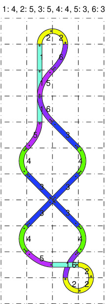
(a) A non-constructible circuit

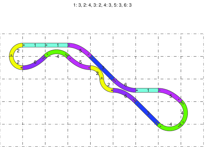
(b) A constructible circuit

Figure 13. Two circuits.

In Figure 13(a), we chose three examples of non-disjoint pieces, covering the three cases seen above. In contrast, in Figure 13(b), the circuit is constructible with three squares in which two disjoint pieces appear each time.

3.5. Adopted definitions

Definition 3.6 (perfectly looping walk).

We will call a perfectly looping walk, a path $\Gamma$ of class $\mathcal{C}^{1}$ in $\mathbb{R}^{2}$, defined in Section 2.1. This path is defined up to isometries, up to a cyclic permutations and up to direction of travel. In an abuse of terminology, we will also call a perfectly looping walk that which allows us to define the path $\Gamma$, i.e, any of:

• the sequence of the centres of the squares ${(c_{i})}_{1\leq i\leq N}$ occupied by the path $\Gamma$, satisfying all of the constraints given in sections 3.2, 3.3 and 3.4, this sequence being defined up to isometries, up to cyclic permutations and up to direction of travel;

• the sequence of angles ${(\alpha_{i})}_{1\leq i\leq N}$ defined in sections 3.1 and 3.2, this sequence being defined up to multiplication by $-1$, up to cyclic permutations and up to direction of travel;

• The sequence of signed piece numbers ${(p_{i})}_{1\leq i\leq N}$ defined in Section 3.1, this sequence being defined up to exchange of $\pm 5$ with $\mp 6$, up to cyclic permutations and up to direction of travel.

Note as well that a perfectly looping walk depends on $N_{j}$ and on the width $e$ which, in this article, is chosen to be less than the critical width equal to the maximum of $e_{0}$ defined by (2) and $\delta_{\min}$ defined by (14) and (15). In the slightly different case where $e>e_{0}$, $e$ must remain less than $1/2$; in the latter case, the connection rules, given in Section 3.4, are to be modified, which is also taken into account in the algorithms used. If we decide to include the pieces of types 7 and 8, $e_{0}$ is then given by (3). .

Definition 3.7 (circuit).

In the remainder of this article, a circuit is therefore the set of geometric pieces which is based on the geometric construction of a perfectly looping walk.

3.6. Computational limitations and algorithmic complexity

In [Jen04], the number of self-avoiding walks was able to be exactly determined up to $N=71$; the author obtained $4$ $190$ $893$ $020$ $903$ $935$ $054$ $619$ $120$ $005$ $916$ paths! In [CJ12], the number of self-avoiding polygons could be exactly determined up to $N=130$; the author obtains $17$ $076$ $613$ $429$ $289$ $025$ $223$ $970$ $687$ $974$ $244$ $417$ $384$ $681$ $143$ $572$ $320$ polygons! Unfortunately, as noted above, these parallelizable methods could not be implemented here. All of the algorithms presented have been programmed in Matlab ®. Two versions were planned: the first is vectorial (and therefore parallelizable), and avoids the use of loops, which is relatively fast. However, the tables used are quickly of a significant size, as well as the total number of circuits to be studied. Up to $N=9$, these calculations are possible. Beyond that, the memory size is too great. It is necessary to move on to calculations with loops, which are much longer, but which avoid the storage of large tables corresponding to possible circuits. Up to $N=11$, the calculations are reasonable. Beyond $N=11$, more than $4$ days of calculation were required (see Section 3.9), and the calculations were not carried out.

The exhaustive enumeration of possible circuits makes use of Cartesian products of finite sets, and is therefore of complexity $\mathcal{O}(A^{N})$, which, in any case, limits computer calculations in theory.

In [Sla11, Jen03, JG99, Gut12a, Gut12, CJ12], an estimation of the number of self-avoiding polygons is given for $N\to+\infty$:

$$q(N)\thicksim A\mu^{N}N^{\gamma-1},$$ (17)

where $\mu$ is called the connective constant, $\gamma$ a critical exponent and $A$ a critical amplitude. The proposed value of $\mu$ is the same as the one corresponding to self-avoiding walks (see [Jen03]):

$$\mu\approx 2.638.$$ (18a)

The value of $$\gamma$$ corresponding to square lattices is given by

$$\gamma-1\approx-\frac{5}{2},$$ (18b)

and finally, we have (see [Jen03])

$$A\approx 0.0795774715.$$ (19)

The estimation (17) cannot be used here as is, since we have seen that the search for self-avoiding walks and polygons is not identical. Nevertheless, we will improperly use this approximation to evaluate the number of circuits for larger values of $N$ in Section 4.

Remark 3.8.

As in the generalization of Remark 2.1, we note that, in [Jen04a, tableau 3], Jensen proposes the following value of $\mu$ in the case of Kagomé lattice:

$$\mu\approx 2.560.$$ (20)

3.7. Some examples of the enumeration of circuits

We reconsider some examples similar to Example 3.2, this time using all of the proposed circuit selection algorithms.

Example 3.9.

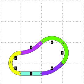
(a)

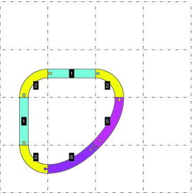
(b)

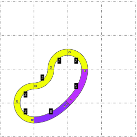
(c)

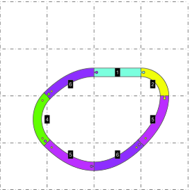
(d)

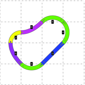
(e)

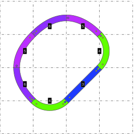
(f)

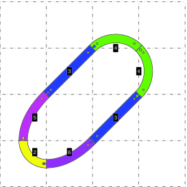
(g)

Figure 14. All of the 7 circuits kept from the set of 50000 possible circuits.

If we draw all the feasible circuits with $N=7$ pieces and $N_{j}=+\infty$, we obtain the $7$ circuits in Figure 14. In this figure, only the circuits which are all different up to an isometry have been drawn.

Example 3.10.

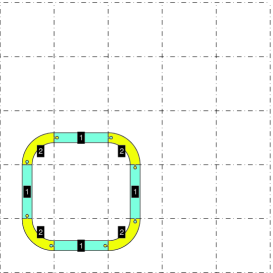
(a)

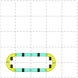
(b)

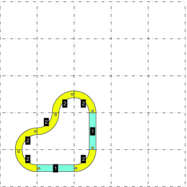
(c)

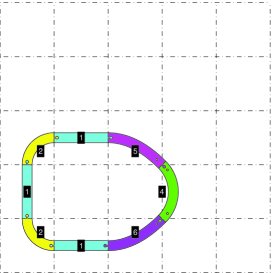
(d)

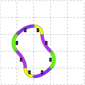
(e)

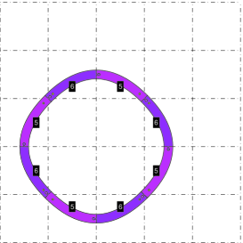
(f)

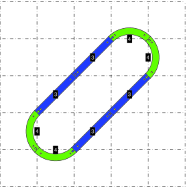
(g)

(h)

(i)

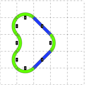
(j)

Figure 15. 10 of the 33 circuits retained from the set of 250000 possible circuits.

If we draw some of the feasible circuits with $N=8$ pieces and $N_{j}=+\infty$, we obtain the $10$ circuits in Figure 15. In this figure, only the circuits which are all different up to an isometry have been drawn. Note that Figures 15(a), 15(b) and 15(c) correspond to circuits which are used only the parts 1 et 2. We shall return to these particular circuits.

Example 3.11.

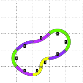
(a)

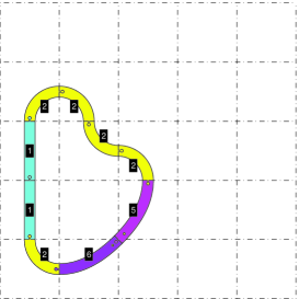
(b)

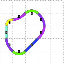
(c)

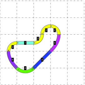
(d)

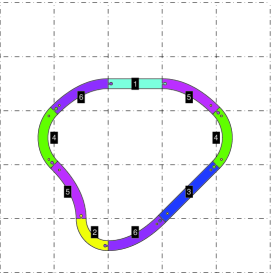
(e)

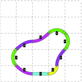
(f)

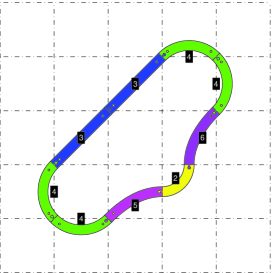
(g)

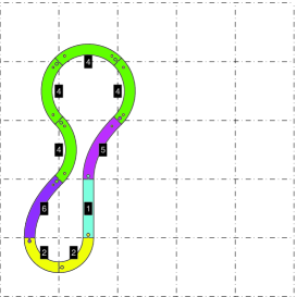
(h)

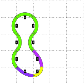
(i)

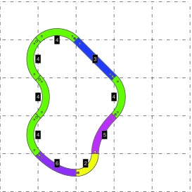
(j)

Figure 16. 10 of the 74 circuits retained from the set of 1250000 possible circuits.

If we draw some of the feasible circuits with $N=9$ pieces and $N_{j}=+\infty$, we obtain the $10$ circuits in Figure 16. In this figure, only the circuits which are all different up to an isometry have been drawn. For several among them, one may observe some pieces which belong to the same square being disjoint.

Example 3.12.

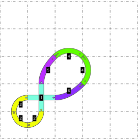
(a)

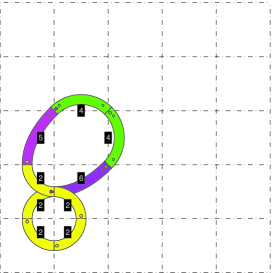
(b)

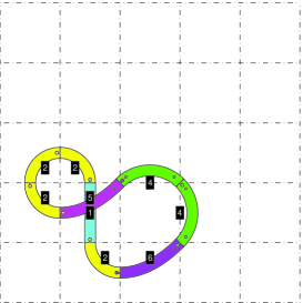
(c)

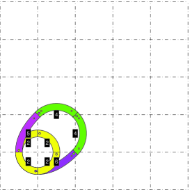
(d)

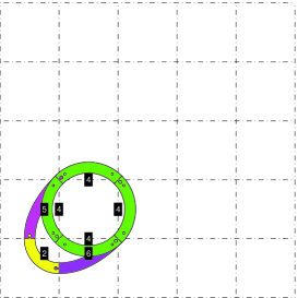
(e)

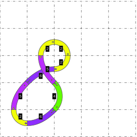
(f)

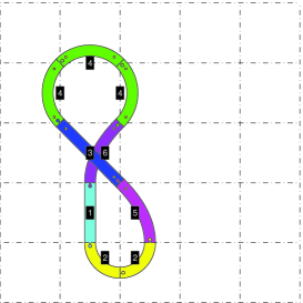
(g)

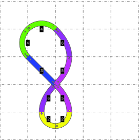
(h)

(i)

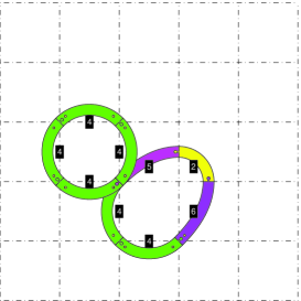
(j)

Figure 17. 10 of the 18 circuits retained from the set of 1250000 possible circuits.

If we draw some of the feasible circuits with $N=9$ pieces and $N_{j}=+\infty$, we obtain the $10$ circuits in Figure 17. In this example we content ourselves to keep only the non-constructible circuits, which remain permissible since all of the algorithms have been implemented computationally.

Example 3.13.

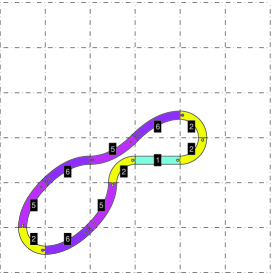
(a)

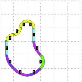
(b)

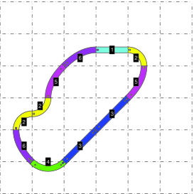
(c)

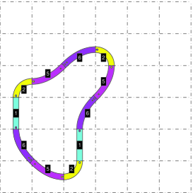
(d)

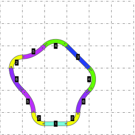
(e)

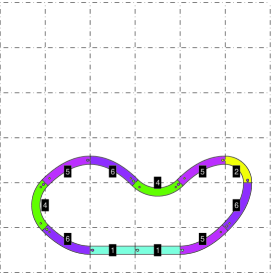
(f)

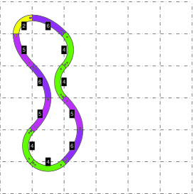
(g)

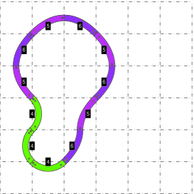
(h)

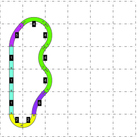
(i)

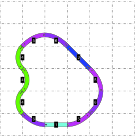
(j)

Figure 18. 10 of the 753 circuits retained from the set of 31250000 possible circuits.

We conclude with the calculation corresponding to the maximal value of $N$ which can be reasonably calculated computationally.

If we draw some of the feasible circuits with $N=11$ pieces and $N_{j}=4$, which corresponds to the toy-box distributed by Easyloop, we obtain the $10$ circuits in Figure 18.

3.8. Comparison with traditional systems and the classical theory of self-avoiding polygons (square tiling)

Traditional systems, such as Brio ®, offer a multitude of shapes of track pieces, which are all circular or straight, but never parabolic. See http://www.woodenrailway.info/track/trackmath.html. Naturally, one cannot compare the studied circuits with these types of system, which do not offer designs which can be varied, scaled and modulated at will. However, in some such systems there exist in particular eighths of a circle, which assembled in pairs gives a quarter-circle, whose radius is equal to one of the lengths of the straight track pieces. In other words, the pieces of the studied systemsnumbered 1 and 2, used alone, allow the creation of simple circuits which could be created with the traditional systems. These circuits have straight pieces which can only be perpendicular to each other. The forms are less varied and above all, the number of possible circuits offered is much smaller than those of our system (see Sections 3.9 and 4).

We now choose to show a circuit formed solely from pieces 1 and 2. We note that, in this case, adjacent squares may only have one common side, and that this is very close to the case of self-avoiding polygons, but pieces in the same square may also coexist. We also note that the number of pieces used is necessarily even, exactly in the case of self-avoiding polygons.

Example 3.14.

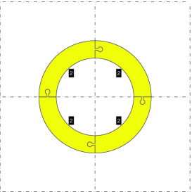
Figure 19. The sole circuit kept from the set of 400 possible circuits.

We draw the sole feasible circuit with $N=4$ pieces. We choose $N_{j}=+\infty$ if $j\in\{1,2\}$, and zero otherwise. We obtain the $1$ circuits in Figure 19.

Example 3.15.

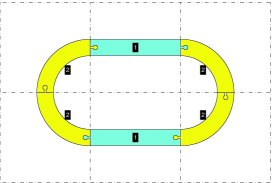
Figure 20. The sole circuit kept from the set of 10000 possible circuits.

As in the example 3.14, we draw the sole feasible circuit with $N=6$ pieces. We choose also $N_{j}=+\infty$ if $j\in\{1,2\}$, and zero otherwise. We obtain the $1$ circuits in Figure 20.

Example 3.16.

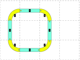
(a)

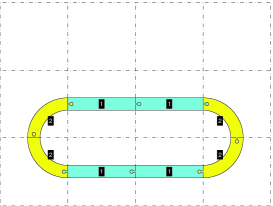
(b)

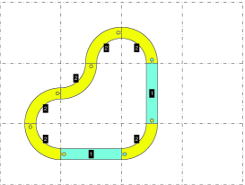
(c)

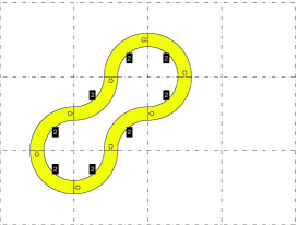
(d)

Figure 21. All of the 4 circuits kept from the set of 250000 possible circuits.

As in the example 3.14, we draw all the feasible circuits with $N=8$ pieces. We obtain the $4$ circuits in Figure 21. Note that we find naturally some of circuits with $8$ pieces of Example 3.10 (see Figures 15(a), 15(b) and 15(c)).

Example 3.17.

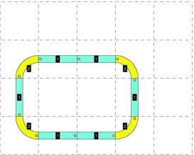
(a)

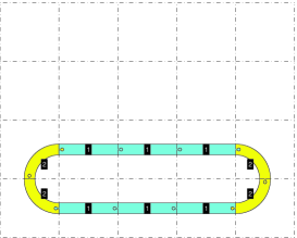
(b)

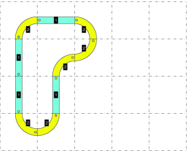
(c)

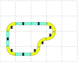
(d)

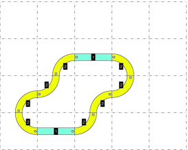
(e)

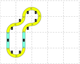
(f)

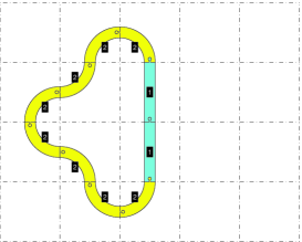
(g)

Figure 22. All of the 7 circuits kept from the set of 6250000 possible circuits.

As in the example 3.14, we draw all the feasible circuits with $N=10$ pieces. We obtain the $7$ circuits in Figure 22.

3.9. Determination of the number of circuits

$N$	possible circuits	looping circuits	direct isom.	isometries	constructible
$1$	$2$	$0$	$0$	$0$	$0$
$2$	$16$	$0$	$0$	$0$	$0$
$3$	$80$	$0$	$0$	$0$	$0$
$4$	$400$	$4$	$4$	$2$	$2$
$5$	$2000$	$10$	$2$	$1$	$1$
$6$	$10000$	$36$	$10$	$5$	$5$
$7$	$50000$	$140$	$20$	$7$	$7$
$8$	$250000$	$664$	$107$	$41$	$33$
$9$	$1250000$	$2988$	$332$	$92$	$74$
$10$	$6250000$	$13910$	$1466$	$428$	$304$
$11$	$31250000$	$64592$	$5872$	$1512$	$986$

Table 2. Numbers of circuits corresponding to $N_{j}=+\infty$

In Table 2, we give in succession (for $N_{j}=+\infty$).

• the number of possible circuits examined, from which only those which form a loop were retained;

• the number of looping circuits;

• the number of looping circuits, up to a direct isometry;

• the number of looping circuits, up to any isometry;

• and finally, the number of looping circuits, up to any isometry, and only keeping constructible circuits.

We note that for values of $N$ smaller than $3$, no circuits exist. For values of $N$ smaller than $7$, all of the circuits are constructible.

$N$	looping circuits	direct isom.	isometries	constructible
$4$	$4$	$4$	$2$	$2$
$5$	$10$	$2$	$1$	$1$
$6$	$36$	$10$	$5$	$5$
$7$	$126$	$18$	$6$	$6$
$8$	$564$	$89$	$30$	$28$
$9$	$2358$	$262$	$72$	$63$
$10$	$10710$	$1126$	$324$	$244$
$11$	$45034$	$4094$	$1046$	$753$

Table 3. The (non-zero) numbers of circuits corresponding to $N_{j}=4$

In Table 3 we give the (non-zero) numbers of circuits corresponding to the distributed Easyloop boxes, where $N_{j}=4$. We note that up to $6$, the values for $N_{j}=4$ and $N_{j}=+\infty$ are equal.

$N$	Self-avoiding polygons	traditional Brio system	Easyloop system
$4$	$1$	$1$	$2$
$5$	$0$	$0$	$1$
$6$	$2$	$1$	$5$
$7$	$0$	$0$	$6$
$8$	$7$	$4$	$28$
$9$	$0$	$0$	$63$
$10$	$28$	$7$	$244$
$11$	$0$	$0$	$753$

Table 4. The numbers of self-avoiding polygons, the (non-zero) numbers of circuits for traditional Brio system and the Easyloop system

Finally, in Table 4, the numbers of self-avoiding polygons, corresponding to a square lattice (see [MS93, table p. 396]) or http://oeis.org/A002931/b002931.txt and a comparison between traditional systems (see Section 3.8) and the Easyloop system are proposed. For the Easyloop system, only the number of constructible circuits up to an isometry is displayed. The number $N_{j}$ equals $12$ if $j=1,2$, and zero otherwise.

Traditional circuits are very close to self-avoiding polygons, except for the following two differences already mentioned above: the permitted isometries are all the isometries of a square, and a square may be used multiple times by the circuit. The common point is that for $N$ odd, the number obtained is zero.

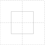
Figure 23. The sole circuit with 4 pieces, drawn under polygons form.

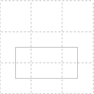
Figure 24. The sole circuit with 6 pieces, drawn under polygons form.

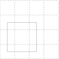
(a)

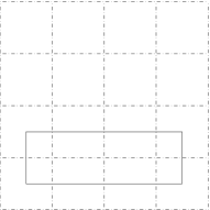
(b)

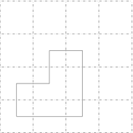
(c)

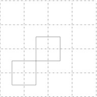
(d)

Figure 25. The 4 circuits with 8 pieces, drawn under polygons form.

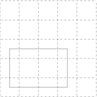
(a)

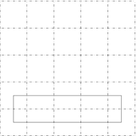
(b)

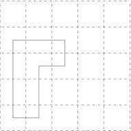
(c)

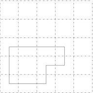
(d)

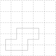
(e)

(f)

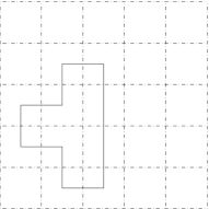
(g)

Figure 26. The 7 circuits with 10 pieces, drawn under polygons form.

We draw the circuits obtained in examples 3.14, 3.15, 3.16 and 3.17 in the form of closed polygons. See Figures 23, 24, 25 and 26 respectively.

• For $N=4$ (see Figure 23), we obtain in both cases, 1 circuit.

• For $N=6$ (see Figure 24), we obtain 1 traditional circuit and two self-avoiding polygons, rectangular in shape. The latter two correspond to the traditional circuit and its image under a rotation by angle $\pi/2$.

• For $N=8$ (see Figure 25), we obtain 4 traditional circuits and 7 self-avoiding polygons. As noted in http://oeis.org/A002931, the 7 self-avoiding polygons correspond to the 1, 2 and 4 rotations (by angle $\pi/2$) of the circuits in Figures 25(a) 25(b) and 25(c) respectively. The circuit in Figure 25(d) does not correspond to any self-avoiding polygon, since one of the squares is occupied by two pieces. We have thus indeed found $7=1+2+4$.

• For $N=10$ (see Figure 26), we obtain 7 traditional circuits and 28 self-avoiding polygons. In fact, the two circuits in Figures 26(a) and 26(b) each provide, by 2 rotations (by angle $\pi/2$), 2 self-avoiding polygons. The 2 circuits in Figures 26(c) and 26(d) each provide, by 4 rotations (by angle $\pi/2$) and one reflection, 8 self-avoiding polygons. The circuit in Figure 26(e) provides, by one rotation (by angle $\pi/2$) and one reflection, 4 self-avoiding polygons. The circuit in Figure 26(g), provides, by 4 rotations (by angle $\pi/2$), 4 self-avoiding polygons. The circuit in Figure 26(f) does not correspond to any self-avoiding polygon, since one of the squares is occupied by two pieces. We have thus indeed found $28=2\times 2+2\times 2\times 4+4+4$ self-avoiding polygons.

If one now compares the last column of Table 4 with the first two, one notices that the comparison is then in favor of the Easyloop system.

The number of operations is

$$\mathcal{O}\left(5^{N}\right)$$ (21)

Thus, passing from $N$ to $N+1$ multiplies the number of operations by $5$. All of the results in this section were realized in a time greater than $23$ hours. Replacing $11$ by $12$ therefore demands more than $4$ days of calculation!

4. Estimation of the number of circuits with a significant number of pieces

In the case where $N$ is greater than $11$, the calculations take too long, and it is not possible to use the enumeration of the circuits. We use, with much impropriety, the estimation given by (17), which comes from [Sla11, Jen03, JG99, Gut12a, Gut12, CJ12]. We will take the number of circuits given in Section 3.9, and we will make use of it to evaluate the constants $A$, $\mu$ and $\gamma$ in formula (17). This evaluation is replaced by an equality and the coefficients $A$, $\mu$ and $\gamma$ are determined by solving a least squares system, which becomes linear when we take the logarithm.

	looping circuits	direct isom.	isometries	constructible
$\gamma-1$	$-4.41060$	$-10.08120$	$-9.74233$	$-8.75998$
$\mu$	$7.68523$	$13.10739$	$11.22176$	$9.13739$

Table 5. The values of $\gamma-1$ and $\mu$ obtained using Table 2 (corresponding to $N_{j}=+\infty$).

Let us now estimate $\gamma-1$ and $\mu$ using the different results from Table 2 (corresponding to $N_{j}=+\infty$). See Table 5. The obtained values are naturally different from the values given in (18). This is normal since the estimation (17) has been replaced by an equality, and naturally, nothing a priori validates this equality. We note that the signs of the coefficients are consistent with those in the literature.

	looping circuits	direct isom.	isometries	constructible
$\gamma-1$	$-3.93476$	$-9.65660$	$-9.76067$	$-8.69817$
$\mu$	$6.80151$	$11.68005$	$10.61788$	$8.69023$

Table 6. The values of $\gamma-1$ and $\mu$ obtained using Table 2 (corresponding to $N_{j}=4$).

If we now do the estimation of $\mu$ using the different results in Table 3 (corresponding to $N_{j}=4$), we obtain the values given in Table 6, with some observations similar to the previous ones.

To validate our method, we can give the retained values of the coefficients $A$, $\mu$ and $\gamma-1$ in formula (17) by using the values from the identification obtained by taking the first column of Table 4. They are given by

$$A=2.1356,\quad\gamma-1=-3.87223,\quad\mu=3.15940,$$

which are on the order of the values obtained by (18). For $N=24$, we obtain a value of $102070280$ for the number of perfectly looping walks , instead of the value $2$ $521$ $270$, given in the literature.

The retained values of the coefficients $A$, $\mu$ and $\gamma-1$ in formula (17) in the case of the Easyloop boxes, corresponding to $N_{j}=4$, therefore correspond to the last case in Table 6 and are given by

$$A=4.5900\,10^{1},\quad\gamma-1=-8.69817,\quad\mu=8.69023.$$ (22)

In case (22), the estimated numbers of circuits are then $\left\{0,0,0,2,2,3,8,21,65,226,857\right\}$, which is close to the exact numbers of circuits ($\left\{0,0,0,2,1,5,6,28,63,244,753\right\}$). For $N=24$, we obtain

$$q(24)\approx 1560511691458.$$ (23)

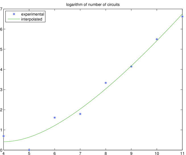
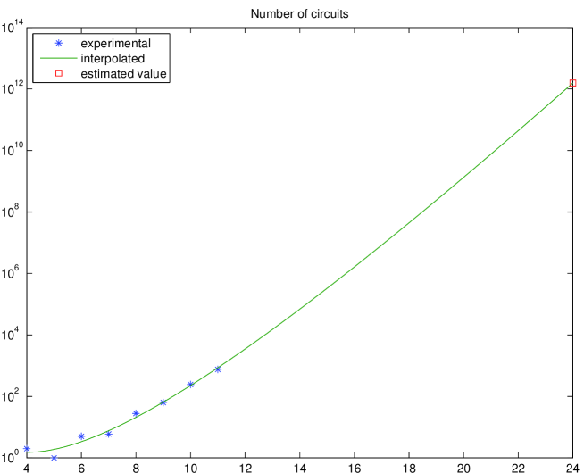
Figure 27. Estimation of the number of circuits in the case $N_{j}=4$.

We then obtain the curves shown in Figure 27.

To compare the Easyloop circuits with traditional systems, one may likewise use the numbers in the last column of Table 4, which gives

$$\mu=2.52246,$$ (24)

$\gamma-1=-3.71496$ and an estimated number of circuits equal to

$$q(24)\approx 130229,$$ (25)

which is still much smaller than (23).We note that the case (24), the closest to that of self-avoiding polygons, provides values relatively close to those given by (18a).

5. Random construction of circuits with a large number of pieces

For values of $N$ smaller than $11$, we are capable of obtaining all of the constructible circuits, and in particular to show them. Another objective of a manufacturer would be to offer a catalogue of train-track designs which may contain circuits with any $N$. Unfortunately, beyond $N=11$, this is no longer conceivable. Manual designs are possible, but tiresome, and non-programmable. We thus propose in this section a way to automatically generate circuits for given $N$ and $N_{j}$ for values larger than $N=11$, without having to create all of the possible circuits as proposed in Section 3.2, by relying on a random method.

For a given $N\geq 1$, we consider $r,s\in\mathbb{N}^{*}$ such that $N=r+s$. We are capable of determining all of the circuits with $r$ pieces starting from the origin by describing a Cartesian product of finite sets. To avoid this long stage, we will simply randomly choose $q$ circuits by choosing the parameters in this Cartesian product. For each of these circuits, the last square occupied by the last piece, is not necessarily equal to the origin. We take $R\in\mathbb{N}^{*}$ and we keep from these circuits only those for which the absolute value of the abscissa and the ordinate is less than $R$. For each of these retained circuits, we are capable of determining all of the circuits with $s$ pieces starting from the last square and returning to the origin. We therefore consider all of the circuits obtained by the concatenation of the circuits with $r$ pieces going from the origin to any square with the circuits with $s$ pieces returning to the origin. Finally, of these circuits, we keep only those for which they types of pieces are less than $N_{j}$. We also apply the selection of the isometries and the constructibility constraints. One has hence obtained a certain number of circuits constructible with $N$ pieces, without having had to to construct the Cartesian product of the circuit parameters determining all of the possible circuits, whose cardinality is too great. Naturally, to increase the chances of success, one must choose $r$, $s$, $q$ and $R$ as large as possible. Computationally, it is necessary that these numbers not be too great. The random determination will therefore consist of choosing these parameters appropriately. One may create such circuits oneself using the executables distributed for Windows, quoted on page 1.

Example 5.1.

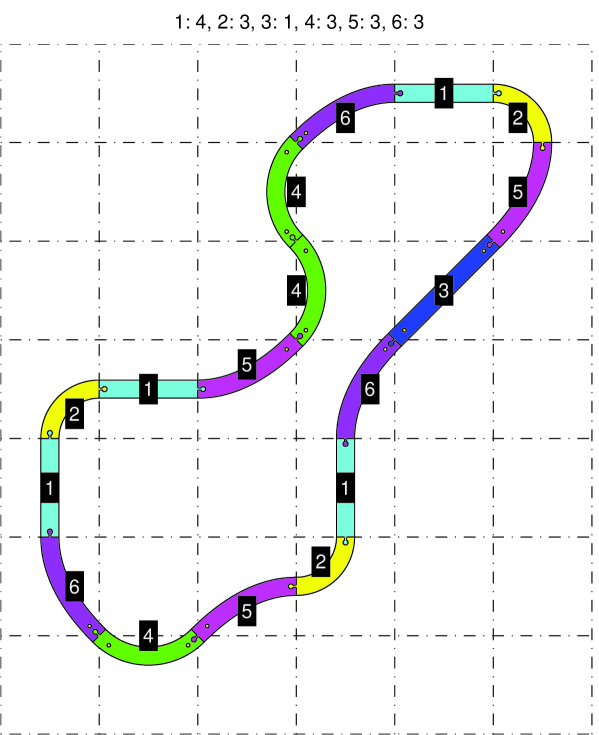
Figure 28. A random circuit with $17$ pieces.

We choose $N_{j}=4$ and the following parameters

$$r=12,\quad s=5,\quad q=18,\quad R=8.$$

We obtain the random circuit with $17$ pieces given in Figure 28.

We have obtained some circuits in a random way, being able to take values of $N$ strictly larger than $11$, and, finally, in a much shorter time.

Other circuits created randomly with this method are available on the internet (see page 1).

6. Generalizations

6.1. Shape of the tiling

We have seen that for a square tiling, the number of curves necessary to connect each point of ${\mathcal{H}}_{i}$ to every other distinct point in ${\mathcal{H}}_{i}$ was equal to 5 or 6, according to whether or not one takes the pieces numbered 7 and 8. This number depends intrinsically on the number of points in ${\mathcal{H}}_{i}$ and on the cardinality of the group of the isometries leaving the square invariant.

The question arises whether or not the method of constructing the rails of the studied circuits can be applied to types of tiling other than the square, and if one is capable of determining the number of basic curves, here equal to 5 or 6, uniquely from the tiling and the points ${\mathcal{H}}_{i}$ considered. This generalization is also mentioned for self-avoiding walks in [Jen04a], which is a simpler case since the circuits may only follow the edges of the tiles constituting the tiling of the plane.

(a) : with the 3 middles

(b) : with the 3 middles and the 3 vertices

Figure 29. Other possible tilings: the equilateral triangle

For example, one may consider tiling the plane with equilateral triangles, taking only the 3 middles of the 3 sides (see Figure 29(a)) or the 3 middles and the 3 vertices of the triangle (see Figure 29(b)). We impose that the curve passes through two distinct points of this set ${\mathcal{H}}_{i}$, while being tangent to the straight line connecting this point with the center of the triangle. In the first case, a single curve is necessary, while in the second, 3 are. Other solutions can be envisaged, with other types of possible tilings.

Can the number of necessary curves be expressed as a function of the tiling polygon and the nature of the points ${\mathcal{H}}_{i}$? The enumeration of circuits, constructed using these methods, seems once again to be an open problem.

6.2. Presence of switches

We keep to the case of square tiling. As described earlier, if the presence of switches is not anticipated, the pieces of constructible circuits must not have extremities in common. One can, on the contrary, allow certain extremities be common to several pieces, which simply corresponds to allowing switches.

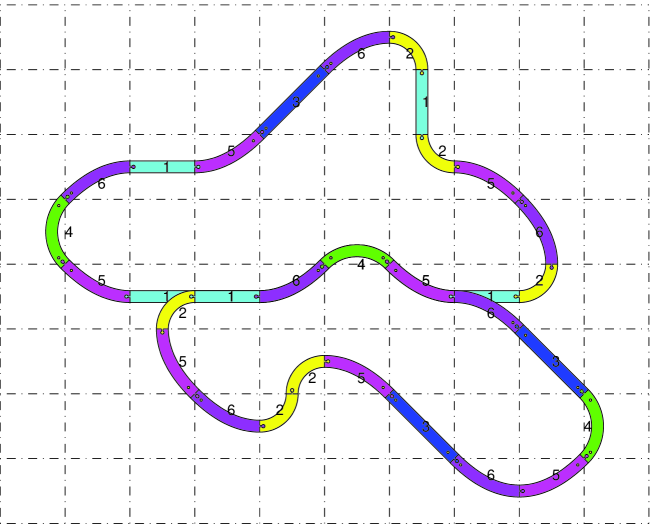
Figure 30. An example track design with 2 switches

In this case, the oriented circuits may contain several loops, which makes them directed graphs, whose enumeration is a much more arduous problem due to the multiplicity of the types of possible switches and therefore the types of possible graphs. See Figure 30, which shows an example of a circuit with switches.

7. Conclusion

The question << Is it possible to tally all of the circuits which can be realized from a given number of pieces? >> is simple to express, and more difficult to resolve. We have succeeded in this article: the enumeration and the construction of such circuits is possible and have been implemented computationally up to $N=11$. Beyond that, an estimation of the number of possible circuits has been provided (see (23), corresponding to the case $N_{j}=4$, and (25)). We note that these numbers correspond to the number of circuits which contain exactly $24$ pieces. If we want to tally all of the circuits which contain at most $24$ pieces, it is sufficient to sum the last column in Table 3, which gives $1102$ circuits, then to apply the estimation for $N$ varying from $12$ to $24$, with the estimated parameters given by (22), which gives in total

$$1873804310490,$$ (26)

that is, a total of more than

$$\numberstringnum{1} 24$$ trillion feasible circuits with pieces. (27)

In addition, a random circuit construction has been offered, allowing values of $N$ strictly larger than $N=11$ to be obtained. Some executables and a catalogue of circuits are available online.

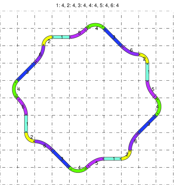
Figure 31. An example track design with $24$ pieces.

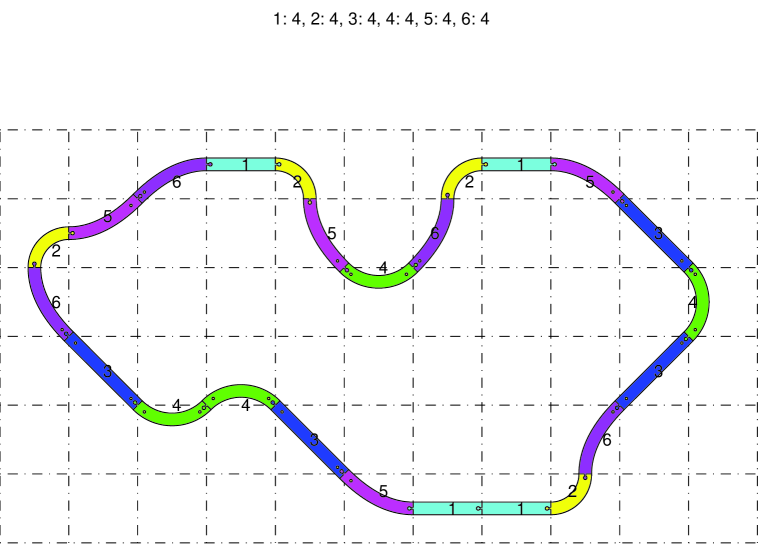
Figure 32. An example track design with $24$ pieces.

Finally, we note that two constructible circuits corresponding to $N_{j}=4$, and containing exactly the maximum number of pieces ($24$) have been created by hand. See Figures 31 and 32.

It is interesting that the traditional theory of self-avoiding paths corresponds almost to existing trains circuits (see section 3.8) while the patend studied system corresponds to the notion of perfectly looping walk.

It remains to improve the circuit enumeration algorithms to obtain higher values of $N$, in the deterministic case, by trying, for example, to avoid the very long enumeration of possible circuits; is a direct construction of constructible circuits possible, without going through this enumeration? An application of the parallelizable techniques proposed by G. Slade, I. Jensen, or A. J. Guttmann might be tried on the circuits in order to increase the values of $N$ for which the circuit enumerations are exact.

It would be interesting to prove if estimation (17) is valid, with an eventual calculation of the constants $A$, $\mu$ and $\gamma$. The generalization raised in Section 6 allows the creation of other types of circuits, but also an attempt to understand the algebraic nature of the system proposed with squares.

References

- Université Lyon IUniversité Lyon I[Bas12] Université Lyon I Jérôme Bastien “Circuit apte à guider un véhicule miniature” Patent published on the website of the INPI http://bases-brevets.inpi.fr/fr/document/FR2990627.html?p=6&s=1423127185056&cHash=cfbc2dad6e2e39808596f86b89117583, 2012
- [Bas13] Jérôme Bastien “Circuit suitable for guiding a miniature vehicle [Circuit apte à guider un véhicule miniature]” International patent published under the Patent Cooperation Treaty. See http://bases-brevets.inpi.fr/fr/document/WO2013171170.html?p=6&s=1423127405077&cHash=6947975351b6d1cf7dd56d4e749a98bb, 2013
- [Bas15] Jérôme Bastien “ Comment concevoir un circuit de train miniature qui se reboucle toujours bien ? – Deux questions d’algèbre et de dénombrement (French) [How to design a miniature train circuit that loops always good? – Two questions algebra and counting]” Slides presented at the << séminaire détente >> de la Maison des Mathématiques et de l’Informatique, Lyon, available on the web: http://utbmjb.chez-alice.fr/recherche/brevet_rail/expose_MMI_2015.pdf, 2015 URL: http://utbmjb.chez-alice.fr/recherche/brevet_rail/expose_MMI_2015.pdf
- [Bas15a] Jérôme Bastien “ Comment concevoir un circuit de train miniature qui se reboucle toujours bien ? (French) [How to design a miniature train circuit that loops always good?]” Slides presented at the Forum of mathematics in 2015 at the Academy of Sciences, Literature and Arts in Lyon, available on the web: http://utbmjb.chez-alice.fr/recherche/brevet_rail/expose_forum_2015.pdf, 2015 URL: http://utbmjb.chez-alice.fr/recherche/brevet_rail/expose_forum_2015.pdf
- [CJ12] Nathan Clisby and Iwan Jensen “A new transfer-matrix algorithm for exact enumerations: self-avoiding polygons on the square lattice” In J. Phys. A 45.11, 2012, pp. 115202, 15 DOI: 10.1088/1751-8113/45/11/115202
- [FHK02] “Handbook of computer aided geometric design” North-Holland, Amsterdam, 2002, pp. xxviii+820
- [Gut12] Anthony J. Guttmann “Self-Avoiding Walks and Polygons – An Overview”, 2012 arXiv: http://arxiv.org/abs/1212.3448
- [Gut12a] Anthony J. Guttmann “Self-Avoiding Walks and Polygons – An Overview” http://www.asiapacific-mathnews.com/02/0204/0001_0010.pdf In Asia Pacific Mathematics Newsletter 2.4, 2012
- [HM13] Frédéric Holweck and Jean-Noël Martin “ Géométries pour l’ingénieur (french) [Geometries for the engineer]” Paris: Ellipses, 2013
- [Jen03] Iwan Jensen “A parallel algorithm for the enumeration of self-avoiding polygons on the square lattice” In J. Phys. A 36.21, 2003, pp. 5731–5745 DOI: 10.1088/0305-4470/36/21/304
- [Jen04] Iwan Jensen “Enumeration of self-avoiding walks on the square lattice” In J. Phys. A 37.21, 2004, pp. 5503–5524 DOI: 10.1088/0305-4470/37/21/002
- [Jen04a] Iwan Jensen “Improved lower bounds on the connective constants for two-dimensional self-avoiding walks” In J. Phys. A 37.48, 2004, pp. 11521–11529 DOI: 10.1088/0305-4470/37/48/001
- [JG99] Iwan Jensen and Anthony J. Guttmann “Self-avoiding polygons on the square lattice” In J. Phys. A 32.26, 1999, pp. 4867–4876 DOI: 10.1088/0305-4470/32/26/305
- [LH97] Camille Lebossé and Corentin Hémery “ Géométrie. Classe de Mathématiques (Programmes de 1945) (French) [Geometry. Classe de Mathématiques (1945 programs)]” Paris: Jacques Gabay, 1997
- [MS93] Neal Madras and Gordon Slade “The self-avoiding walk”, Probability and its Applications Birkhäuser Boston, Inc., Boston, MA, 1993, pp. xiv+425
- [Per] Daniel Perrin “ Les courbes de Bézier (French) [Bézier curves]” Notes for preparing the CAPES mathematics available sur http://www.math.u-psud.fr/~perrin/CAPES/geometrie/BezierDP.pdf
- [Sla11] Gordon Slade “The self-avoiding walk: a brief survey” In Surveys in stochastic processes, EMS Ser. Congr. Rep. Eur. Math. Soc., Zürich, 2011, pp. 181–199 DOI: 10.4171/072-1/9