ENCODING ARGUMENTS

Many proofs in discrete mathematics and theoretical computer science are based on the probabilistic method. To prove the existence of a good object, we pick a random object and show that it is bad with low probability. This method is effective, but the underlying probabilistic machinery can be daunting. “Encoding arguments” provide an alternative presentation in which probabilistic reasoning is encapsulated in a “uniform encoding lemma”. This lemma provides an upper bound on the probability of an event using the fact that a uniformly random choice from a set of size $n$ cannot be encoded with fewer than $\log_{2}n$ bits on average. With the lemma, the argument reduces to devising an encoding where bad objects have short codewords.

In this expository article, we describe the basic method and provide a simple tutorial on how to use it. After that, we survey many applications to classic problems from discrete mathematics and computer science. We also give a generalization for the case of non-uniform distributions, as well as a rigorous justification for the use of non-integer codeword lengths in encoding arguments. These latter two results allow encoding arguments to be applied more widely and to produce tighter results.

1 Introduction

There is no doubt that probability theory plays a fundamental role in computer science. Often, the fastest and simplest solutions to important algorithmic and data structuring problems are randomized [26, 30]; average-case analysis of algorithms relies entirely on tools from probability theory [36]; many difficult combinatorial questions have strikingly simple solutions using probabilistic arguments [2].

Unfortunately, many of these beautiful results present a challenge to most computer scientists, as they rely on advanced mathematical concepts. For instance, the 2013 edition of ACM/IEEE Curriculum Guidelines for Undergraduate Degree Programs in Computer Science does not require a full course in probability theory [1, Page 50]. Instead, the report recommends a total of 6 Tier-1 hours and 2 Tier-2 hours on discrete probability, as part of the discrete structures curriculum [1, Page 77].

“Encoding arguments” offer a more elementary approach to presenting these results. We transform the task of upper-bounding the probability of a specific event, $\mathcal{E}$, into the task of devising a code for the set of elementary events in $\mathcal{E}$. This provides an alternative to performing a traditional probabilistic analysis or, since we are only concerned with finite spaces, to directly estimating the size of $\mathcal{E}$. Just as the probabilistic method is essentially only a sophisticated rephrasing of a counting argument with many theoretical and intuitive advantages, encoding arguments likewise offer their own set of benefits, although they are also just a glorified way of counting. More specifically:

1. Except for applying a simple Uniform Encoding Lemma, encoding arguments are “probability-free.” There is no danger of common mistakes such as multiplying probabilities of non-independent events or (equivalently) multiplying expectations.

   The actual proof of the Uniform Encoding Lemma is trivial. It only uses the probabilistic fact that if we have a finite set $X$ with $r$ special elements and we pick an element from $X$ uniformly at random, the probability of selecting a special element is $r/|X|$.

2. Encoding arguments usually yield strong results; $\Pr\{\mathcal{E}\}$ typically decreases at least exponentially in the parameter of interest. Traditionally, these strong results require (at least) careful calculations on probabilities of independent events and/or concentration inequalities. This latter subject is advanced enough to fill entire textbooks [7, 13].

3. Encoding arguments are natural for computer scientists. They turn a probabilistic analysis into the task of designing an efficient code—an algorithmic problem. Consider the following two problems:

   1. Prove an upper-bound of $1/n^{\log n}$ on the probability that a random graph on $n$ vertices contains a clique of size $k=\lceil 4\log n\rceil$.

   2. Design an encoding for graphs on $n$ vertices so that any graph with a clique of size $k=\lceil 4\log n\rceil$ is encoded using at most $\binom{n}{2}-\log^{2}n$ bits. (Note: Your encoding and decoding algorithms don’t have to be efficient, just correct.)

   Many computer science undergraduates would not know where to start on the first problem. Even a good student who realizes that they can use Boole’s Inequality will still be stuck wrestling with the formula $\binom{n}{4\log n}2^{-\binom{4\log n}{2}}$.

We believe that encoding arguments are an easily accessible, yet versatile tool for solving many problems. Most of these arguments can be applied after learning almost no probability theory beyond the Encoding Lemma mentioned above.

The remainder of this article is organized as follows. In Section 2, we present an elementary tutorial on the method, including the Uniform Encoding Lemma, the basis of most of our encoding arguments. In Section 3, we review more advanced mathematical tools, such as entropy, Stirling’s Approximation, and encoding schemes for natural numbers. In Section 4 we show how the Uniform Encoding Lemma can be applied to Ramsey graphs, several hashing variants, expander graphs, analysis of binary search trees, and $k$-SAT. In Section 5, we introduce the Non-Uniform Encoding Lemma, a generalization that extends the reach of the method, This is demonstrated in Section 6, where we prove the Chernoff bound and consider percolation and random triangle counting problems. Section 7 presents an alternative view of encoding arguments, justifying the use of non-integer codeword lengths. Section 8 concludes the survey.

2 An Elementary Tutorial

This section gives a simple tutorial on the basic method.

2.1 Basic Definitions, Prefix-free Codes and the Uniform Encoding Lemma

Before we can talk about codes, we first recall some basic definitions about bit strings.

• binary string/bit string: a finite (possibly empty) sequence of elements from $\{0,1\}$. The set of all bit strings is denoted by $\{0,1\}^{*}$.

  Examples: $0$; $1$; $101$; $00101$; $1010$; $1101$; $\varepsilon$ (the empty string).

• length of a bit string $x$: the number of bits in $x$, denoted by $|x|$.
  Examples: $|0|=1$; $|1|=1$; $|101|=3$; $|00101|=5$.

• $n_{0}(x),n_{1}(x)$: the number of $0$- and $1$-bits in a bit string $x$.

  Examples: $n_{0}(010)=2$; $n_{1}(010)=1$; $n_{0}(1111)=0$; $n_{1}(1111)=4$.

• $n$-bit string: a bit string of length $n$, for $n\in\mathbb{N}$. The set of all $n$-bit strings is denoted by $\Sigma^{n}$.

  Examples: $001$ is a $3$-bit string; $00101$ is a $5$-bit string; $\Sigma^{2}=\{00,01,10,11\}$.

• prefix: a bit string $x\in\Sigma^{*}$ is a prefix of another binary string $y\in\Sigma^{*}$ if $y$ is of the form $y=xz$, for some $z\in\Sigma^{*}$. Here, $xz$ denotes the bit string obtained by concatenating $x$ with $z$.

  Example: $0$, $01$, $010$, and $0100$ are prefixes of $0100$, but $1$ and $00$ are not.

Next, we explain our coding theoretic vocabulary. In the following, let $X$ be a finite or countable set.

• code for $X$/encoding of $X$: an injective function $C\colon X\to\{0,1\}^{*}$ that assigns a unique finite bit string to every element of $X$.
  Example: Let $X=\{a,b,c\}$. The function $C:a\mapsto 01,b\mapsto 1110,c\mapsto 10$ is a code for $X$, but the function $C^{\prime}:a\mapsto 01,b\mapsto 1110,c\mapsto 01$ is not.

• codewords of a code $C\colon X\to\{0,1\}^{*}$: the elements of the range of $C$.

  Example: The codewords of $C:a\mapsto 01,b\mapsto 1110,c\mapsto 10$ are $01$, $1110$, and $10$.

• partial code $C\colon X\nrightarrow\{0,1\}^{*}$ for $X$: a code that is only a partial function, i.e., not every element in $X$ is assigned a codeword. We will use the convention that $|C(x)|=\infty$ if $x$ is not in the domain of $C$.

  Example: Let $X=\{a,b,c\}$. Then $C:a\mapsto 01,b\mapsto 1110$ is a partial code for $X$ in which there is no codeword for $c$. We have $|C(a)|=2$, $|C(b)|=4$, and $|C(c)|=\infty$.

• prefix-free (partial) code: a (partial) code $C$ in which no codeword is the prefix of another codeword.

  Examples: The code $C_{1}:a\mapsto 10,b\mapsto 111,c\mapsto 01$ is prefix-free. The code $C_{2}:a\mapsto 10,b\mapsto 111,c\mapsto 1011$ is not prefix-free, because the codeword for $a$ is a prefix of the codeword for $c$.

• fixed-length code for a finite set $X$: a prefix-free code for $X$ where each codeword has length $\lceil\log|X|\rceil$. It is obtained by enumerating the elements of $X$ in some order $x_{0},x_{1},\ldots,x_{|X|-1}$ and assigning to each $x_{i}$ the binary representation of $i$, padded with leading zeros to obtain $\lceil\log|X|\rceil$ bits.

  Example: Let $X=\{a,b,c,d,e\}$. Then, a possible fixed-length code for $X$ is $C:a\mapsto 000,b\mapsto 001,c\mapsto 010,d\mapsto 011,e\mapsto 100$.

It is helpful to visualize prefix-free codes as (rooted ordered) binary trees whose leaves are labelled with the elements of $X$. The codeword for a given $x\in X$ is obtained by tracing the root-to-leaf path leading to $x$ and outputting a 0 each time this path goes from a parent to its left child, and a 1 each time it goes to a right child. (See Figure 1.)

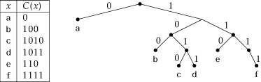
Figure 1: A prefix-free code for $X=\{\mathtt{a},\mathtt{b},\mathtt{c},\mathtt{d},\mathtt{e},\mathtt{f}\}$ and the corresponding leaf-labelled binary tree (which can also be viewed as a partial prefix-free code for $\{\mathtt{a},\mathtt{b},\mathtt{c},\ldots,\mathtt{z}\}$).

We claim that if a code $C$ is prefix-free, then for any $k\in\mathbb{N}$, the code $C$ has not more than $2^{k}$ codewords of length at most $k$. To see this, we modify $C$ into a code $\widehat{C}$, in which every codeword of length $\ell<k$ is extended to a word of length exactly $k$ by appending $k-\ell$ zeros. Since $C$ is prefix-free, $\widehat{C}$ is a valid code, i.e., all codewords of $\widehat{C}$ are pairwise distinct. Furthermore, the number of codewords in $C$ with length at most $k$ equals the number of codewords in $\widehat{C}$ of length exactly $k$. Since all codewords of length $k$ in $\widehat{C}$ are pairwise distinct, there are at most $2^{k}$ of them. To illustrate the proof, consider the code $C:a\mapsto 0,b\mapsto 100,c\mapsto 1010,d\mapsto 1011,e\mapsto 110,f\mapsto 1111$ from Figure 1. Our claim says that $C$ has at most $2^{3}=8$ codewords of length at most $3$. The modified code $\widehat{C}$ is as follows. $\widehat{C}:a\mapsto 000,b\mapsto 100,c\mapsto 1010,d\mapsto 1011,e\mapsto 110,f\mapsto 1111$. We see that $\widehat{C}$ is indeed a code, and its codewords of length exactly $3$ are in correspondence with the codewords of length at most $3$ in $C$, as claimed.

Finally, we need to review some probability theory.

• probability distribution $p$ on $X$: a function $p:X\rightarrow[0,1]$ with $\sum_{x\in X}p(x)=1$. We sometimes write $p_{x}$ instead of $p(x)$. We again emphasize that $X$ is a finite or countable set.

  Example: for $X=\{a,b,c\}$, the function $p:a\mapsto 1/3,b\mapsto 1/2,c\mapsto 1/6$ is a probability distribution, but $p^{\prime}:a\mapsto 1/3,b\mapsto 1/2,c\mapsto 1/5$ is not. For $X=\{1,2,\dots\}$, the function $p(x)=1/2^{x}$ is a probability distribution.

• uniform distribution on finite set $X$: the probability distribution $p:X\rightarrow[0,1]$ given by $p_{x}=1/|X|$, for all $x\in X$.

• Bernoulli distribution on $n$-bit strings with parameter $\alpha\in[0,1]$: the probability distribution $p$ on $X=\{0,1\}^{n}$ with $p_{x}=(1-\alpha)^{n_{0}(x)}\alpha^{n_{1}(x)}$. In other words, a bit string $x$ is sampled by setting each bit to $1$ with probability $\alpha$ and to $0$ with probability $1-\alpha$, independently of the other bits. We write $\mathrm{Bernoulli}(\alpha)$ for $p$.

The following lemma provides the foundation on which this survey is built. The lemma is folklore, but as we will see in the following sections, it has an incredibly wide range of applications and can lead to surprisingly powerful results.

Lemma 1 (Uniform Encoding Lemma).

Let $X$ be a finite set and $C\colon X\nrightarrow\{0,1\}^{*}$ a partial prefix-free code. If an element $x\in X$ is chosen uniformly at random, then

$$\Pr\{|C(x)|\leq\log|X|-s\}\leq 2^{-s}\enspace.$$

Proof.

We call a codeword of $C$ short if it has length at most $k=\lfloor\log|X|-s\rfloor$. Above, we observed that $C$ has at most $2^{k}$ short codewords. Since $C$ is injective, each codeword has at exactly one preimage in $X$. Since $x$ is chosen uniformly at random from $X$, the probability that it is the preimage of a short codeword is at most

$$\frac{2^{k}}{|X|}\leq\frac{2^{\log|X|-s}}{|X|}=2^{-s}\enspace.$$

∎

2.2 Runs in Binary Strings

To finish our tutorial, we give a simple use of the Uniform Encoding Lemma. Let $x$ be a bit string. A run in $x$ is a consecutive sequence of one bits. For example, $0110111101011111$ contains runs of length $2$, $4$, $1$, and $5$, and every substring of a run is also a run. We now show that a $n$-bit string that is chosen uniformly at random is unlikely to contain a run of length significantly more than $\log n$. (See Figure 2.)

Figure 2: Illustration of Theorem 1 and its proof.

Theorem 1.

Let $x=(x_{1},\ldots,x_{n})\in\{0,1\}^{n}$ be chosen uniformly at random and let $t={\left\lceil{\lceil\log n\rceil}+s\right\rceil}$. Then, the probability that $x$ contains a run of length $t$ is at most $2^{-s}$.

Proof.

We construct a partial prefix-free code for strings with a run of length $t$. For such a string $x=(x_{1},\ldots,x_{n})$, let $i$ be the minimum index with $x_{i}=x_{i+1}=\cdots=x_{i+t-1}=1$. The codeword $C(x)$ for $x$ is the binary string that consists of the (${\lceil\log n\rceil}$-bit binary encoding of the) index $i$ followed by the $n-t$ bits $x_{1},\dots,x_{i-1},x_{i+t},\dots,x_{n}$. (See Figure 2.) For example, for $n=8$ and $t=4$, we encode $x=10111110$ as $010\,10\,10$, since the first run of length $4$ in $x$ is at position $2$, which is $010$ as a $3=\lceil\log 8\rceil$-bit number.

Observe that $C(x)$ has length

$$|C(x)|={\lceil\log n\rceil}+n-t\leq n-s\enspace.$$

To see that $C$ is injective, we argue that we can obtain $(x_{1},\ldots,x_{n})$ uniquely from $C(x)$: The first ${\lceil\log n\rceil}$ bits from $C(x)$ tell us, in binary, a position $i$ for which $x_{i}=x_{i+1}=\dots=x_{i+t-1}=1$; the following $n-t$ bits in $C(x)$ contain the remaining bits $x_{1},x_{2},\dots,x_{i-1},x_{i+t},x_{i+t+1},\dots,x_{n}$. Thus, $C$ is a partial code whose domain are the $n$-bit strings with a run of length $t$. Also, $C$ is prefix-free, as all codewords have the same length. Recall from our convention that $|C(x)|=\infty$ if $x$ does not have a run of length $t$.

Now, there are $2^{n}$ $n$-bit strings. Therefore, by the Uniform Encoding Lemma, the probability that a uniformly random $n$-bit string has a run of length $t$ is at most

$$\Pr\{|C(x)|\leq n-s\}\leq 2^{-s}\enspace.$$

∎

The proof of Theorem 1 contains the main ideas used in most encoding arguments:

1. The arguments usually show that a particular bad event is unlikely. In Theorem 1 the bad event is the occurrence of a substring of $t$ consecutive ones.

2. We use a partial prefix-free code whose domain is the bad event, whose elements we call the bad outcomes. In this case, the code $C$ only encodes strings containing a run of length $t$, and a particular such string is a bad outcome.

3. The code begins with a concise description of the bad outcome, followed by a straightforward encoding of the information that is not implied by the bad outcome. In Theorem 1, the bad outcome is completely described by the index $i$ at which the run of length $t$ begins, and this implies that the bits $x_{i},\ldots,x_{i+t-1}$ are all equal to 1, so these bits can be omitted in the second part of the codeword.

2.3 A Note on Ceilings

Note that Theorem 1 also has an easy proof using the union bound: If we let $\mathcal{E}_{i}$ denote the event $x_{i}=x_{i+1}=\cdots=x_{i+t}=1$, then

$$\Pr\left\{\bigcup_{i=0}^{n-t-1}\mathcal{E}_{i}\right\} \leq\sum_{i=0}^{n-t-1}\Pr\{\mathcal{E}_{i}\}$$ (using the union bound)

$$=\sum_{i=0}^{n-t-1}2^{-t} x_{i}$$ (using the independence of the ’s)

$$\leq n2^{-t} n-t\leq n$$ (the sum has identical terms)

$$\leq n2^{-\lceil\log n\rceil-s} t$$ (using the definition of )

$$\leq 2^{-s}\enspace. *$$ ()

This traditional proof also works with the sometimes smaller value $t={\lceil\log n+s\rceil}$ (note the lack of a ceiling over $\log n$), in which case the final inequality ($*$) holds with an equality.

In the encoding proof of Theorem 1, the ceiling on the $\log n$ is an artifact of encoding the integer $i$ which comes from a set of size $n$. When sketching an encoding argument, we think of this as requiring $\log n$ bits. However, when the time comes to write down a careful proof we need a ceiling over this term as bits are a discrete quantity.

In Section 7, however, we will formally justify that the informal intuition we use in blackboard proofs is actually valid; we can think of the encoding of $i$ using $\log n$ bits even if $\log n$ is not an integer. In general we can imagine encoding a choice from among $r$ options using $\log r$ bits for any $r\in\mathbb{N}$. From this point onwards, we omit ceilings this way in all our theorems and proofs. This simplifies calculations and provides tighter results. For now, it allows us to state the following cleaner version of Theorem 1:

Theorem 1b.

Let $x\in\{0,1\}^{n}$ be chosen uniformly at random and let $t={\lceil\log n+s\rceil}$. Then, the probability that $x$ contains a run of length $t$ is at most $2^{-s}$.

3 More Background and Preliminaries

3.1 Encoding Sparse Bit Strings

At this point we should also point out an extremely useful trick for encoding sparse bit strings. For any $\alpha\in(0,1)$, there exists a code $C_{\alpha}\colon\{0,1\}^{n}\rightarrow\{0,1\}^{*}$ such that, for any bit string $x\in\{0,1\}^{n}$ having $n_{1}(x)$ ones and $n_{0}(x)$ zeros,

$$|C_{\alpha}(x)|=\left\lceil n_{1}(x)\log\frac{1}{\alpha}+n_{0}(x)\log\frac{1}{1-\alpha}\right\rceil\enspace.$$ (1)

This code is the Shannon-Fano code for $\mathrm{Bernoulli}(\alpha)$ bit strings of length $n$ [17, 37]. More generally, for any probability density $p:X\to[0,1]$, there is a Shannon-Fano code $C:X\to\{0,1\}^{*}$ such that

$$|C(x)|={\lceil\log(1/p_{x})\rceil}\enspace.$$

Moreover, we can construct such a code deterministically, even when $X$ is countably infinite.

Again, as explained in Section 7, we can omit the ceiling in the expression for $|C_{\alpha}(x)|$. This holds for any value of $n$. In particular, for $n=1$, it gives a “code” for a single bit where the cost of encoding a 1 is $\log(1/\alpha)$ and the cost of encoding a 0 is $\log(1/(1-\alpha))$. Indeed, the “code” for bit strings of length $n>1$ is what we get when we apply this 1-bit code to each bit of the bit string.

If we wish to encode bit strings of length $n$ and we know in advance that the strings contain exactly $k$ one bits, then we can obtain an optimal code by taking $\alpha=k/n$. The resulting fixed length code has length

$$k\log(n/k)+(n-k)\log(n/(n-k))\enspace.$$ (2)

Formula (2) brings us to our next topic: binary entropy.

3.2 Binary Entropy

The binary entropy function $H\colon(0,1)\to(0,1]$ is defined by

$$H(\alpha)=\alpha\log(1/\alpha)+(1-\alpha)\log(1/(1-\alpha))$$

and it will be quite useful. The binary entropy function and two upper bounds on it that we derive below are illustrated in Figure 3.

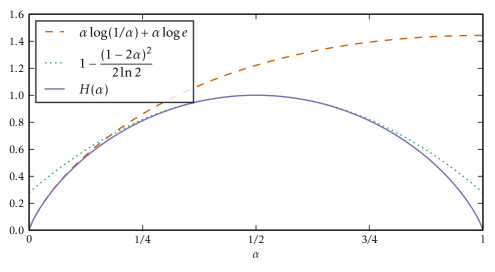
Figure 3: Binary entropy, $H$, and two useful approximations.

We have already encountered a quantity that can be expressed in terms of the binary entropy. From (2), a bit string of length $n$ with exactly $k$ one bits can be encoded with a fixed-length code of $nH(k/n)$ bits.

The binary entropy function can be difficult to work with, so it is helpful to have some manageable approximations. One of these is derived as follows:

$$H(\alpha) =\alpha\log(1/\alpha)+(1-\alpha)\log(1/(1-\alpha))=\alpha\log(1/\alpha)+(1-\alpha)\log(1+\alpha/(1-\alpha))$$

$$\leq\alpha\log(1/\alpha)+(1-\alpha)\cdot\alpha/(1-\alpha)\log e\leq\alpha\log(1/\alpha)+\alpha\log e$$ (3)

since $1+x\leq e^{x}$ for all $x\in\mathbb{R}$. Inequality (3) is a useful approximation when $\alpha$ is close to zero, in which case $H(\alpha)$ is also close to zero.

For $\alpha$ close to $1/2$ (in which case $H(\alpha)$ is close to 1), we obtain a good approximation from the Taylor series expansion at $1/2$. Indeed, a simple calculation shows that

$$H^{\prime}(\alpha)=\log(1/\alpha)-\log(1/(1-\alpha))$$

and that

$$H^{(i)}(\alpha)=\frac{(i-2)!}{\ln 2}\left(\frac{(-1)^{i-1}}{\alpha^{i-1}}-\frac{1}{(1-\alpha)^{i-1}}\right),$$

for $i\geq 2$. Hence, $H^{(i)}(1/2)=0$, for $i\geq 1$ odd, and

$$H^{(i)}(1/2)=-\frac{(i-2)!\,2^{i}}{\ln 2},$$

for $i\geq 2$ even. The Taylor series expansion at $1/2$ now gives

$$H(1/2+\beta) =H(1/2)+\sum_{i=1}^{\infty}\frac{H^{(i)}(1/2)}{i!}\beta^{i}=1-\frac{1}{\ln 2}\sum_{i=1}^{\infty}\frac{(2i-2)!2^{2i}}{(2i)!}\beta^{2i}=1-\frac{1}{2\ln 2}\sum_{i=1}^{\infty}\frac{(2\beta)^{2i}}{i(2i-1)}.$$

In particular, for $$\beta=\varepsilon/2$$,

$$H\left(\frac{1+\varepsilon}{2}\right) =1-\frac{1}{2\ln 2}\sum_{i=1}^{\infty}\frac{\varepsilon^{2i}}{i(2i-1)}<1-\frac{\varepsilon^{2}}{2\ln 2}\enspace.$$ (4)

3.3 Basic Chernoff Bound

With all the pieces in place, we can now give an encoding argument for a well-known and extremely useful result typically attributed to Chernoff [10].

Theorem 2.

Let $x\in\{0,1\}^{n}$ be chosen uniformly at random. Then, for any $\varepsilon\geq 0$,

$$\Pr\left\{n_{1}(x)\leq(1-\varepsilon)\frac{n}{2}\right\}\leq e^{-\varepsilon^{2}n/2}\enspace.$$

Proof.

Encode the bit string $x$ using a Shannon-Fano code $C_{\alpha}$ with $\alpha=(1-\varepsilon)/2$. Then, the length of the codeword for $x$ is

$$|C_{\alpha}(x)|=n_{1}(x)\log(1/\alpha)+n_{0}(x)\log(1/(1-\alpha))\enspace.$$

Since $\alpha<1/2$, we have $\log(1/\alpha)>\log(1/(1-\alpha))$, so for fixed $n$, the codeword length $|C_{\alpha}(x)|$ is increasing in $n_{1}(x)$ and becomes maximal when $n_{1}(x)$ is maximal. Thus, if $n_{1}(x)\leq\alpha n$, then

$$|C_{\alpha}(x)|\leq\alpha n\log(1/\alpha)+(1-\alpha)n\log(1/(1-\alpha))=nH(\alpha)\leq n\left(1-\frac{\varepsilon^{2}}{2\ln 2}\right)=n-s\enspace,$$

where the second inequality is an application of (4), and where $s=\varepsilon^{2}n/(2\ln 2)$. Now, $x$ was chosen uniformly at random from a set of size $2^{n}$. By the Uniform Encoding Lemma, we obtain that

$$\Pr\{n_{1}(x)\leq\alpha n\}\leq\Pr\{|C_{\alpha}(x)|\leq n-s\}\leq 2^{-s}=e^{-\varepsilon^{2}n/2}\enspace.$$

∎

In Section 6.1, after developing a Non-Uniform Encoding Lemma, we will extend this argument to $\mathrm{Bernoulli}(\alpha)$ bit strings.

3.4 Factorials and Binomial Coefficients

Before moving on to some more advanced encoding arguments, it will be helpful to remind the reader of a few inequalities that can be derived from Stirling’s Approximation of the factorial [35]. Recall that Stirling’s Approximation states that

$$n!=\left(\frac{n}{e}\right)^{n}\sqrt{2\pi n}\left(1+\varTheta\left(\frac{1}{n}\right)\right)\enspace.$$ (5)

In many cases, we are interested in representing a set of size $n!$ using a fixed-length code. By (5), and using once again that $1+x\leq e^{x}$ for all $x\in\mathbb{R}$ as well as $1+x\geq e^{x/2}$ for $x\in[0,1/2]$, the length of the codewords in such a code is

$$\log n! =n\log n-n\log e+(1/2)\log n+\log\sqrt{2\pi}+\log(1+\varTheta(1/n))$$

$$=n\log n-n\log e+(1/2)\log n+\log\sqrt{2\pi}+\varTheta(1/n)$$

$$=n\log n-n\log e+\varTheta(\log n)\enspace.$$ (6)

We are sometimes interested in codes for the $\binom{n}{k}$ subsets of $k$ elements from a set of size $n$. Note that there is an easy bijection between such subsets and binary strings of length $n$ with exactly $k$ ones. Therefore, we can represent these using the Shannon-Fano code $C_{k/n}$ and each of our codewords will have length $nH(k/n)$. In particular, this implies that

$$\log\binom{n}{k}\leq nH(k/n)\leq k\log n-k\log k+k\log e$$ (7)

where the last inequality is an application of (3). The astute reader will notice that we just used an encoding argument to prove an upper-bound on $\binom{n}{k}$ without using the formula $\binom{n}{k}=\frac{n!}{k!(n-k)!}$. Alternatively, we could obtain a slightly worse bound by applying (5) to this formula.

3.5 Encoding the Natural Numbers

So far, we have only explicitly been concerned with codes for finite sets. In this section, we give an outline of some prefix-free codes for the set of natural numbers. Of course, if $p:\mathbb{N}\to[0,1]$ is a probability density, then the Shannon-Fano code for $p$ could serve. However, it seems easier to simply design our codes by hand, rather than find appropriate distributions.

A code is prefix-free if and only if any message consisting of a sequence of its codewords can be decoded unambiguously and instantaneously as it is read from left to right: Consider some sequence of codewords $M=y_{1}y_{2}\cdots y_{k}$ from a prefix-free code $C$. Since $C$ is prefix-free, then $C$ has no codeword $z$ which is a prefix of $y_{1}$, so reading $M$ from left to right, the first codeword of $C$ which we recognize is precisely $y_{1}$. Continuing in this manner, we can decode the whole message $M$. Conversely, if for each codeword $y$ of $C$, a message consisting of this single codeword can be decoded unambiguously and instantaneously from left to right, we know that $y$ has no prefix among the codewords of $C$, i.e. $C$ is prefix-free. This idea allows us to more easily design the codes in this section, which were originally given by Elias [14].

The unary encoding of an integer $i\in\mathbb{N}$, denoted by $U(i)$, begins with $i$ 1 bits which are followed by a 0 bit. This code is not particularly useful in itself, but it can be improved as follows: The Elias $\gamma$-code for $i$, denoted by $E_{\gamma}(i)$, begins with the unary encoding of the number of bits in $i$, and then the binary encoding of $i$ itself (minus its leading bit). The Elias $\delta$-code for $i$, denoted by $E_{\delta}(i)$ begins with an Elias $\gamma$-code for the number of bits in $i$, and then the binary encoding of $i$ itself (minus its leading bit). This process can be continued recursively to obtain the Elias $\omega$-code, which we denote by $E_{\omega}$. Each of these codes has a decoding procedure as in the preceding paragraph, which establishes their prefix-freeness.

The most important properties of these codes are their codeword lengths:

$$|U(i)| =i+1\enspace,$$

$$|E_{\gamma}(i)| =2\log i+O(1)\enspace,$$

$$|E_{\delta}(i)| =\log i+2\log\log i+O(1)\enspace,$$

$$|E_{\omega}(i)| =\log i+\log\log i+\dots+\underbrace{\log\cdots\log}_{\text{$\log^{*}i$ times}}i+O(\log^{*}i)\enspace.$$

Here, $\log^{*}i$ denotes the number of times we need to apply the function $x\mapsto\log x$ to the integer $i$ until we obtain a number that is smaller than $2$. It may be worth noting that the lengths of unary codes correspond to the lengths of Shannon-Fano codes for a geometric distribution with density $p_{i}=1/2^{i+1}$, that is,

$$\log(1/p_{i})=\log 2^{i+1}=|U(i)|\enspace,$$

and the lengths of Elias $\gamma$-codes correspond to the lengths of Shannon-Fano codes for a discrete Cauchy distribution with density $p_{i}=c/i^{2}$ for a normalization constant $c$, that is,

$$\log(1/p_{i})=2\log i-\log c=|E_{\gamma}(i)|+O(1)\enspace.$$

The lengths of Elias $\delta$-codes and $\omega$-codes do not seem to arise as the lengths of Shannon-Fano codes for any named distributions.

4 Applications of the Uniform Encoding Lemma

We now start with some applications of the Uniform Encoding Lemma. In each case, we will design and analyze a partial prefix-free code $C\colon X\nrightarrow\{0,1\}^{*}$, where $X$ depends on the context.

4.1 Graphs with no Large Clique or Independent Set

The Erdős-Rényi random graph $G_{n,p}$ is the probability space on graphs with vertex set $V=\{1,\ldots,n\}$ in which each edge $\{u,w\}\in\binom{V}{2}$ is present with probability $p$ and absent with probability $1-p$, independently of the other edges. Erdős [15] used the random graph $G_{n,\frac{1}{2}}$ to prove that there are graphs that have neither a large clique nor a large independent set. Here we show how this can be done using an encoding argument.

Theorem 3.

For $n\geq 3$ and $s\in\mathbb{N}$, the probability that $G\in G_{n,\frac{1}{2}}$ contains a clique or an independent set of size $t={\lceil 3\log n+\sqrt{2s}\rceil}$ is at most $2^{-s}$.

Proof.

This encoding argument compresses the $\binom{n}{2}$ bits of $G$’s adjacency matrix, as they appear in row-major order.

Suppose the graph $G$ contains a clique or an independent set $S$ of size $t$. The encoding $C(G)$ begins with a bit indicating whether $S$ is a clique or independent set; followed by the set of vertices of $S$; then the adjacency matrix of $G$ in row major-order, omitting the $\binom{t}{2}$ bits implied by the edges or non-edges in $S$. Such a codeword has length

$$|C(G)|=1+t\log n+\binom{n}{2}-\binom{t}{2}\enspace.$$ (8)

Before diving into the detailed arithmetic, we intuitively argue why we’re heading in the right direction: Roughly, (8) is of the form:

$$|C(G)|=\binom{n}{2}+t\log n-\varOmega(t^{2})\enspace.$$

That is, we need to invest $O(t\log n)$ bits to encode the vertex set of a clique or an independent set of size $t$, but we save $\varOmega(t^{2})$ bits in the encoding of $G$’s adjacency matrix. Clearly, for $t>c\log n$, with $c$ sufficiently large, this has the form

$$|C(G)|=\binom{n}{2}-\varOmega(t^{2})\enspace.$$

At this point, it is just a matter of pinning down the dependence on $c$. A detailed calculation beginning from (8) gives

$$|C(G)|=\binom{n}{2}+1+t\log n-(1/2)(t^{2}-t)=\binom{n}{2}+1-(1/2)(t^{2}-t-2t\log n)\enspace.$$

The function $f(x)=(1/2)(x^{2}-x-2x\log n)-1$ is increasing for $x\geq\log n+1/2$, so recalling that $t={\lceil 3\log n+\sqrt{2s}\rceil}$, we get

$$f(t) \geq f(3\log n+\sqrt{2s})$$

$$=(1/2)(9\log^{2}n+6\sqrt{2s}\log n+2s-3\log n-\sqrt{2s}-6\log^{2}n-2\sqrt{2s}\log n)-1$$

$$=(1/2)(3\log^{2}n+4\sqrt{2s}\log n-3\log n-\sqrt{2s})+s-1\geq s$$

for $n\geq 3$. Therefore, our code has length

$$|C(G)|=\binom{n}{2}-f(t)\leq\binom{n}{2}-s\enspace.$$

Applying the Uniform Encoding Lemma completes the proof. ∎

Remark 1.

The bound in Theorem 3 can be strengthened a little, since the elements of $S$ can be encoded using only $\log\binom{n}{t}$ bits, rather than $t\log n$. With a more careful calculation, using (7), the proof then works with $t=2\log n+O(\log\log n)+\sqrt{s}$. This comes closer to Erdős’s original result, which was at the threshold $2\log n-2\log\log n+O(1)$ [15].

4.2 Balls in Urns

The random experiment of throwing $n$ balls uniformly and independently at random into $n$ urns is a useful abstraction of many questions encountered in algorithm design, data structures, and load-balancing [26, 30]. Here we show how an encoding argument can be used to prove the classic result that, when we do this, every urn contains $O(\log n/\log\log n)$ balls, with high probability.

Theorem 4.

Let $n,s\in\mathbb{N}$, and let $t$ be such that $t\log(t/e)\geq\log n+s$. Suppose we throw $n$ balls independently and uniformly at random into $n$ urns. Then, for sufficiently large $n$, the probability that any urn contains more than $t$ balls is at most $2^{-s}$.

Before proving Theorem 4, we note that, for any constant $\varepsilon>0$ and all sufficiently large $n$, taking

$$t={\left\lceil\frac{(1+\varepsilon)\log n}{\log\log n}\right\rceil}$$

satisfies the requirements of Theorem 4, since then

$$t\log t \geq\frac{(1+\varepsilon)\log n}{\log\log n}\log\left(\frac{(1+\varepsilon)\log n}{\log\log n}\right)=\frac{(1+\varepsilon)\log n}{\log\log n}\left(\log\log n-\log\left(\frac{\log\log n}{1+\varepsilon}\right)\right)$$

$$=(1+\varepsilon)\log n\left(1-\frac{\log\left(\frac{\log\log n}{1+\varepsilon}\right)}{\log\log n}\right)=(1+\varepsilon)\log n-o(\log n)\enspace.$$

Then,

$$t\log(t/e)=t\log t-t\log e=(1+\varepsilon)\log n-o(\log n)\geq\log n+s\enspace,$$

for sufficiently large $n$, as claimed.

Proof of Theorem 4.

For each $i\in\{1,\ldots,n\}$, let $b_{i}$ denote the index of the urn chosen for the $i$-th ball. The sequence $b=(b_{1},\ldots,b_{n})$ is sampled uniformly at random from a set of size $n^{n}$, and this choice will be used in our encoding argument.

Suppose that urn $j$ contains $t$ or more balls. Then, we encode the sequence $b$ with the value $j$ ($\log n$ bits), followed by a code that describes $t$ of the balls in urn $j$ ($\log\binom{n}{t}$ bits), followed by the remaining $n-t$ values in $b$ that cannot be deduced from the preceding information ($(n-t)\log n$ bits). Thus, we get

$$|C(b)| =\log n+\log\binom{n}{t}+(n-t)\log n$$

$$\leq\log n+t\log n-t\log t+t\log e+(n-t)\log n$$ (using (7))

$$=n\log n+\log n-t\log t+t\log e$$

$$\leq n\log n-s t$$ (by the choice of )

$$=\log n^{n}-s$$

bits. We conclude the proof by applying the Uniform Encoding Lemma. ∎

4.3 Linear Probing

Studying balls in urns as in the previous section is useful when analyzing hashing with chaining (see e.g. Morin [27, Section 5.1]). A more practically efficient form of hashing is linear probing. In a linear probing hash table, we hash the elements of the set $X=\{x_{1},\ldots,x_{n}\}$ into a hash table of size $m=cn$, for some fixed $c>1$. We are given a hash function $h:X\to\{1,\ldots,m\}$ which we assume to be a uniform random variable. To insert $x_{i}$, we try to place it at table position $j=h(x_{i})$. If this position is already occupied by one of $x_{1},\ldots,x_{i-1}$, we try table location $(j+1)\bmod m$, followed by $(j+2)\bmod m$, and so on, until we find an empty spot for $x_{i}$. To find a given element $x\in X$ in the hash table, we compute $j=h(x)$, and we start a linear search from position $j$ until we encounter either $x$ or an empty position. Assuming that the hash table has been created by inserting the elements from $X$ successively according to the algorithm above, we want to study the expected search time for some item $x\in X$.

We call a maximal consecutive sequence of occupied table locations a block. (The table locations $m-1$ and $0$ are considered consecutive.)

Theorem 5.

Let $n\in\mathbb{N}$, $c>e$. Suppose that a set $X=\{x_{1},\dots,x_{n}\}$ of $n$ items has been inserted into a hash table of size $m=cn$, using linear probing. Let $t\in\mathbb{N}$, $t\geq 2$, such that

$$(t-1)\log(c/e)-\log t-3\geq s\enspace,$$

and fix some $x\in X$. Then the probability that the block containing $x$ has size exactly $t$ is at most $2^{-s}$.

Proof.

This is an encoding argument for the sequence

$$h=(h(x_{1}),h(x_{2}),\ldots,h(x_{n}))\enspace,$$

that is drawn uniformly at random from a set of size $m^{n}=(cn)^{n}$.

Suppose that $x$ lies in a block with $t$ elements. We encode $h$ by the first index $b$ of the block containing $x$; followed by the $t-1$ elements $y_{1},\dots,y_{t-1}$ of this block (excluding $x$); followed by the hash values of $x$ and of $y_{1},\dots,y_{t-1}$; followed by the $n-t$ hash values for the remaining elements in $X$.

Since the values $h(x),h(y_{1}),h(y_{2}),\ldots,h(y_{t-1})$ are in the range $b,\ldots,b+t-1$ (modulo $m$), they can be encoded using $t\log t$ bits. Therefore, we obtain a codeword of length

$$|C(h)| =\overbrace{\log m}^{b}+\overbrace{\log\binom{n}{t-1}}^{y_{1},\ldots,y_{t-1}}+\overbrace{t\log t}^{h(x),h(y_{1}),\ldots,h(y_{t-1})}+\overbrace{(n-t)\log m}^{\text{everything else}}$$

$$\leq\log m+(t-1)\log n-(t-1)\log(t-1)+(t-1)\log e+t\log t+(n-t)\log m$$ (by (7))

$$=(n-t+1)\log m+(t-1)\log(m/c)+(t-1)\log e+\log(t-1)+t\log(t/(t-1)) m=cn$$ ()

$$\leq n\log m-(t-1)\log c+(t-1)\log e+\log t+3$$

$$=\log m^{n}-(t-1)\log(c/e)+\log t+3\leq\log m^{n}-s\enspace,$$

since we assumed that $t$ satisfies

$$(t-1)\log(c/e)-\log t-3\geq s$$

and since for $t\geq 2$, we have

$$t\log\frac{t}{t-1}=\frac{t}{\ln 2}\ln\left(1+\frac{1}{t-1}\right)\leq\frac{t}{\ln 2}\cdot\frac{1}{t-1}\leq 3.$$

The proof is completed by applying the Uniform Encoding Lemma. ∎

Remark 2.

The proof of Theorem 5 only works if the factor $c$ in the size $m=cn$ of the linear probing hash table is $c>e$. We know from previous analysis that this is not necessary, and that any $c>1$ is sufficient [36, Theorem 9.8]. We leave it as an open problem to find an encoding proof of Theorem 5 that works for any $c>1$.

Corollary 1.

Let $n\in\mathbb{N}$, $c>e$. Suppose that a set $X=\{x_{1},\dots,x_{n}\}$ of $n$ items has been inserted into a hash table of size $m=cn$, using linear probing. Fix some $x\in X$. Then, the expected search time for $x$ in the hash table is $O(1)$.

Proof.

Let $T$ denote the size of the block containing $x$ in the hash table. Let $t_{0}$ be a large enough constant. Then, by Theorem 5, the probability that $T=t+t_{0}$ is at most $2^{-t\log(c/e)/2}$, since then

$$(t+t_{0}-1)\log(c/e)-\log(t+t_{0})-3\geq(t+t_{0})\log(c/e)/2-3\geq t\log(c/e)/2\enspace.$$

Thus, the expected search time for $x$ is

$$\operatorname{\mathrm{E}}\{T\} =\sum_{t=1}^{\infty}t\Pr\{T=t\}=\sum_{t=1}^{t_{0}}t\Pr\{T=t\}+\sum_{t=1}^{\infty}(t+t_{0})\Pr\{T=t+t_{0}\}$$

$$\leq t_{0}+\sum_{t=1}^{\infty}(t+t_{0})2^{-t\log(c/e)/2}=t_{0}+\sum_{t=1}^{\infty}(t+t_{0})(c/e)^{-t/2}=O(1)\enspace.$$

∎

4.4 Cuckoo Hashing

Cuckoo hashing is relatively new hashing scheme that offers an alternative to classic perfect hashing [31]. We present a clever proof, due to Pătraşcu [33], that cuckoo hashing succeeds with probability $1-O(1/n)$ (see also Haimberger [20] for a more detailed exposition of the argument).

We again hash the elements of the set $X=\{x_{1},\ldots,x_{n}\}$. The hash table consists of two arrays $A$ and $B$, each of size $m=2n$, and two hash functions $h,g:X\to\{1,\ldots,m\}$ which are uniform random variables. To insert an element $x$ into the hash table, we insert it into $A[h(x)]$; if $A[h(x)]$ already contains an element $y$, we insert $y$ into $B[g(y)]$; if $B[g(y)]$ already contains some element $z$, we insert $z$ into $A[h(z)]$, etc. If an empty location is eventually found, the algorithm terminates successfully. If the algorithm runs for too long without successfully completing the insertion, then we say that the insertion failed, and the hash table is rebuilt using different newly sampled hash functions. Any element $x$ either is held in $A[h(x)]$ or $B[g(x)]$, so we can search for $x$ in constant time. The following pseudocode describes this procedure more precisely:

$\textsc{Insert}(x):$

1:  if $x=A[h(x)]$ or $x=B[g(x)]$ then

2:     return  

3:  for MaxLoop iterations do

4:     if $A[h(x)]$ is empty then

5:        $A[h(x)]\leftarrow x$

6:        return  

7:     $x\leftrightarrow A[h(x)]$

8:     if $B[g(x)]$ is empty then

9:        $B[g(x)]\leftarrow x$

10:        return  

11:     $x\leftrightarrow B[g(x)]$

12:  $\textsc{Rehash}()$

13:  $\textsc{Insert}(x)$

The threshold ‘MaxLoop’ is to be specified later. To study the performance of insertion in cuckoo hashing, we consider the random bipartite cuckoo graph $G=(A,B,E)$, where $|A|=|B|=m$ and $|E|=n$, with each vertex corresponding either to a location in the array $A$ or $B$ above, and with edge multiset $E=\{(h(x_{i}),g(x_{i})):1\leq i\leq n\}$.

An edge-simple path in $G$ is a path that uses each edge at most once. One can check that if a successful insertion takes at least $2t$ steps, then the cuckoo graph contains an edge simple path with at least $t$ edges. Thus, in bounding the length of edge-simple paths in the cuckoo graph, we bound the worst case insertion time.

Lemma 2.

Let $s\in\mathbb{N}$. Suppose that we insert a set $X=\{x_{1},\dots,x_{n}\}$ into a hash table using cuckoo hashing. Let $G$ be the resulting cuckoo graph. Then, $G$ has an edge-simple path of length at least $s+\log n+O(1)$ with probability at most $2^{-s}$.

Proof.

We encode $G$ by presenting its set of edges. Since each endpoint of an edge is chosen independently and uniformly at random from a set of size $m$, the set of all edges is chosen uniformly at random from a set of size $m^{2n}$.

Suppose some vertex $v\in A\cup B$ is the endpoint of an edge-simple path of length $t$; such a path has $t+1$ vertices and $t$ edges. Each edge in the path corresponds to an element in $X$. In the encoding, we present the indices of the elements in $X$ corresponding to the $t$ edges of the path in order; then, we indicate whether $v\in A$ or $v\in B$; and we give the $t+1$ vertices in order starting from $v$; followed by the remaining $2n-2t$ endpoints of edges of the graph. This code has length

$$|C(G)| =t\log n+1+(t+1)\log m+(2n-2t)\log m$$

$$=2n\log m+t\log n-t\log m+\log m+O(1)$$

$$=\log m^{2n}-t+\log n+O(1) m=2n$$ (since )

$$\leq\log m^{2n}-s$$

for $t\geq s+\log n+O(1)$. We finish by applying the Uniform Encoding Lemma. ∎

This immediately implies that a successful insertion takes time at most $4\log n+O(1)$ with probability $1-O(1/n)$. Moreover, selecting ‘MaxLoop’ to be $4\log n+O(1)$, we see that a rehash happens only with probability $O(1/n)$.

One can prove that the cuckoo hashing insertion algorithm fails if and only if some subgraph of the cuckoo graph contains more edges than vertices, since edges correspond to keys, and vertices correspond to array locations.

Lemma 3.

The cuckoo graph has a subgraph with more edges than vertices with probability $O(1/n)$. That is, cuckoo insertion succeeds with probability $1-O(1/n)$.

Proof.

Suppose that some vertex $v$ is part of a subgraph with more edges than vertices, and in particular a minimal such subgraph with $t+1$ edges and $t$ vertices. Such a subgraph appears exactly as in Figure 4. By inspection, we see that for every such subgraph, there are two edges $e_{1}$ and $e_{2}$ whose removal disconnects the graph into two paths of length $t_{1}$ and $t_{2}$ starting from $v$, where $t_{1}+t_{2}=t-1$.

(a) A cycle with a chord.

(b) Two cycles connected by a path.

Figure 4: The potential minimal subgraphs of the cuckoo graph.

We encode $G$ by giving the vertex $v$ ($\log m$ bits); and presenting Elias $\delta$-codes for the values of $t_{1}$ and $t_{2}$ and for the positions of the endpoints of $e_{1}$ and $e_{2}$ ($O(\log t)$ bits); then the indices of the edges of the above paths in order ($(t-1)\log n$ bits); then the vertices of the paths in order ($(t-1)\log m$ bits); and the indices of the edges $e_{1}$ and $e_{2}$ ($2\log n$ bits); and finally the remaining $2n-2(t+1)$ endpoints of edges in the graph ($(2n-2(t+1))\log n$ bits). Such a code has length

$$|C(G)| =\log m+O(\log t)+(t-1)(\log n+\log m)+2\log n+(2n-2(t+1))\log m$$

$$=2n\log m+(t+1)\log n-(t+2)\log m+O(\log t)$$

$$=2n\log m+(t+1)\log n-(t+2)\log n-t+O(\log t) m=2n$$ (since )

$$\leq\log m^{2n}-\log n+O(1)\enspace.$$

We finish by applying the Uniform Encoding Lemma. ∎

4.5 2-Choice Hashing

We showed in Section 4.2 that if $n$ balls are thrown independently and uniformly at random into $n$ urns, then the maximum number of balls in any urn is $O(\log n/\log\log n)$ with high probability. In 2-choice hashing, each ball is instead given a choice of two urns, and the urn containing the fewer balls is preferred.

More specifically, we are given two hash functions $h,g:X\to\{1,\ldots,m\}$ which are uniform random variables. Each value of $h$ and $g$ points to one of $m$ urns. The element $x\in X$ is added to the urn containing the fewest elements between $h(x)$ and $g(x)$ during an insertion. The worst case search time is at most the maximum number of hashing collisions, or the maximum number of elements in any urn.

Perhaps surprisingly, the simple change of having two choices instead of only one results in an exponential improvement over the strategy of Section 4.2. The concept of 2-choice hashing was first studied by Azar et al. [3], who showed that the expected maximum size of an urn is $\log\log n+O(1)$. Our encoding argument is based on Vöcking’s use of witness trees to analyze 2-choice hashing [39].

Let $G=(V,E)$ be the random multigraph with $V=\{1,\ldots,m\}$, where $m=cn$ for some constant $c>8$, and $E=\{(h(x),g(x)):x\in X\}$. Each edge in $E$ is labeled with the element $x\in X$ that it corresponds to.

Lemma 4.

The probability that $G$ has a subgraph with more edges than vertices is $O(1/n)$.

Proof.

The proof is similar to that of Lemma 3. More specifically, we encode $G$ by giving the same encoding as in Lemma 3. However, since now $G$ is not bipartite, we cannot immediately deduce for an edge $uv$ in the encoding which endpoint corresponds to which hash function. Thus, for each edge $uv$, we store an additional bit indicating whether $u=h(x)$ and $v=g(x)$, or $u=g(x)$ and $v=h(x)$. This needs $t$ additional bits compared to Lemma 3. Our code thus has length

$$|C(G)| =\log m+O(\log t)+(t-1)(\log n+\log m)+2\log n+(2n-2(t+1))\log m+t$$

$$=2n\log m-\log n-t\log c+t+O(\log t)\leq\log m^{2n}-\log n+O(1)\enspace,$$

since $\log c>1$. ∎

Lemma 5.

$G$ has a component of size at least $(2/\log(c/8))\log n+O(1)$ with probability $O(1/n)$.

Proof.

Suppose $G$ has a connected component with $t$ vertices and at least $t-1$ edges. This component has a spanning tree $T$. Pick an arbitrary vertex as the root of $T$. To encode $G$, we first specify a bit string encoding the shape of $T$. This can be done in $2(t-1)$ bits, tracing a pre-order traversal of $T$, where a 0 bit indicates that the path to the next node goes up, and a 1 bit indicates that the path goes down. Then, we encode the $t$ vertices of $T$, in the order as they are first encountered by the pre-order traveral ($t\log m$ bits). Furthermore, for each edge $e=uv$ of $T$, we store $\log n$ bits encoding the element $x\in X$ corresponding to $e$ and a bit indicating whether $u=h(x)$ and $v=g(x)$, or $u=g(x)$ and $v=h(x)$. Again, the edges are stored in the order and direction as they are encountered by the pre-order traversal. As $T$ has $t-1$ edges, this takes $(t-1)(\log n+1)$ bits. Finally we directly encode the remaining $2(n-t+1)$ endpoints of edges in $G$, in $2(n-t+1)\log m$ bits. In total, our code has length

$$|C(G)| =2(t-1)+t\log m+(t-1)(\log n+1)+2(n-t+1)\log m$$

$$=2n\log m+t\log c-\log n+3t-3-2t\log c+2\log n+2\log c m=cn$$ (since )

$$=\log m^{2n}-t\log c+3t+\log n+O(1)\leq\log m^{2n}-s\enspace,$$

as long as $t$ is such that

$$t\geq\frac{s+\log n+O(1)}{\log(c/8)}\enspace.$$

In particular, for $s=\log n$, the Uniform Encoding Lemma tells us that $G$ has a component of size at least $(2/\log(c/8))\log n+O(1)$ with probability $O(1/n)$. ∎

Suppose that when $x$ is inserted, it is placed in an urn with $t$ other elements. Then, we say that the age of $x$ is $a(x)=t$.

Theorem 6.

Fix $c>8$ and suppose we insert $n$ elements into a table of size $cn$ using $2$-choice hashing. With probability $1-O(1/n)$ all positions in the hash table contain at most $\log\log n+O(1)$ elements.

Proof.

Suppose that some element $x$ has $a(x)=t$. This leads to a binary witness tree $T$ of height $t$ as follows: The root of $T$ is the element $x$. When $x$ was inserted into the hash table, it had to choose between the urns $h(x)$ and $g(x)$, both of which contained at least $t-1$ elements; in particular, $h(x)$ has a unique element $x_{h}$ with $a(x_{h})=t-1$, and $g(x)$ has a unique element $x_{g}$ with $a(x_{g})=t-1$. The elements $x_{h}$ and $x_{g}$ become the left and the right child of $x$ in $T$. The process continues recursively. If some element appears more than once on a level, we only recurse on its leftmost occurrence. See Figure 5 for an example.

Figure 5: The tree $T$ is a witness tree for the 2-choice hashing instance with elements $\dots,x_{5},x_{6},x_{7},x_{8},x_{9},x_{10}$ inserted in order and according to the hash functions $h$ and $g$.

Using $T$, we can iteratively define a connected subgraph $G_{T}$ of $G$. Initially, $G_{T}$ consists of the single node in $V$ corresponding to the bucket that contains the root element $x$ of $T$. Now, to construct $G_{T}$, we go through $T$ level by level, starting from the root. For $i=t,\dots,0$, let $L_{i}$ be all elements in $T$ with age $i$, and let $E_{i}=\{(h(x),g(x)):x\in L_{i}\}$ be the corresponding edges in $G$. When considering $L_{i}$, we add to $G_{T}$ all edges in $E_{i}$, together with their endpoints, if they are not in $G_{T}$ already. Since every element appears at most once in $T$, this adds $|L_{i}|$ new edges to $G_{T}$. The number of vertices in $G_{T}$ increases by at most $|L_{i}|$. In the end, $G_{T}$ contains $\sum_{i=0}^{t}|L_{i}|$ edges. Since $G_{T}$ is connected, with probability $1-O(1/n)$, the number of edges in $G_{T}$ does not exceed the number of vertices, by Lemma 4. We assume that this is the case. Since initially $G_{T}$ had one vertex and zero edges, the iterative procedure must add at least $\sum_{i=0}^{t}|L_{i}|-1$ new vertices to $G_{T}$. This means that all nodes in $T$ but one must have two children, so we can conclude that $T$ is a complete binary tree with at most one subtree removed. It follows that $T$ (and hence $G_{T}$) has at least $2^{t}$ vertices. If we choose $t={\lceil\log\log n+d\rceil}$, then $2^{t}\geq 2^{d}\log n$. We know from Lemma 5 that this happens with probability $O(1/n)$ for a sufficiently large choice of the constant $d$. ∎

Remark 3.

The arguments in this section can be refined by more carefully encoding the shape of trees using Cayley’s formula, which says that there are $t^{t-2}$ unrooted labelled trees on $t$ nodes [9]. In particular, an unrooted tree with $t$ nodes and $m$ choices for distinct node labels can be encoded using $\log\binom{m}{t}+(t-2)\log t$ bits instead of $t\log m+2(t-1)$ bits. We would then recover the same results for hash tables of size $m=cn$ with $c>2e$ instead of $c>8$. In fact, it is known that for any $c>0$ searching in 2-choice hashing takes time $1/c+O(\log\log n)$ [6]. We leave it as an open problem to find an encoding argument for this result when $c>0$.

Remark 4.

Robin Hood hashing is another hashing solution which achieves $O(\log\log n)$ worst case running time for all operations [12]. The original analysis is difficult, but might be amenable to a similar approach as we used in this section. Indeed, when a Robin Hood hashing operation takes a significant amount of time, a large witness tree is again implied, which suggests an easy encoding argument. Unfortunately, this approach appears to involve unwieldy hypergraph encoding.

4.6 Bipartite Expanders

Expanders are families of sparse graphs which share many connectivity properties with the complete graph. These graphs have received much research attention, and have led to many applications in computer science. See, for instance, the survey by Hoory, Linial, and Wigderson [22].

The existence of expanders was originally established through probabilistic arguments [32]. We offer an encoding argument to prove that a certain random bipartite graph is an expander with high probability. There are many different notions of expansion. We will consider what is commonly known as vertex expansion in bipartite graphs: For some fixed $0<\alpha\leq 1$, a bipartite graph $G=(A,B,E)$ is called a $(c,\alpha)$-expander if

$$\min_{\begin{subarray}{c}{A^{\prime}\subseteq A}\\ {|A^{\prime}|\leq\alpha|A|}\end{subarray}}\frac{|N(A^{\prime})|}{|A^{\prime}|}\geq c\enspace,$$

where $N(A^{\prime})\subseteq B$ is the set of neighbours of $A^{\prime}$ in $G$. That is, in a $(c,\alpha)$-expander, every set of vertices in $A$ that is not too large is “expanded” by a factor $c$ by taking one step in the graph.

Let $G=(A,B,E)$ be a random bipartite multigraph where $|A|=|B|=n$ and where each vertex of $A$ is connected to three vertices of $B$ chosen independently and uniformly at random (with replacement). The following theorem shows that $G$ is an expander. The proof of this theorem usually involves a messy sum that contains binomial coefficients and probabilities: see, for example, Motwani and Raghavan [30, Theorem 5.3], Pinsker [32, Lemma 1], or Hoory, Linial, and Wigderson [22, Lemma 1.9].

Theorem 7.

There exists a constant $\alpha>0$ such that $G$ is a $(3/2,\alpha)$-expander with probability at least $1-O(n^{-1/2})$.

Proof.

We encode the graph $G$ by presenting its edge set. Since each edge is selected uniformly at random, the graph $G$ is chosen uniformly at random from a set of size $n^{3n}$.

If $G$ is not a $(3/2,\alpha)$-expander, then there is some set $A^{\prime}\subseteq A$ with $|A^{\prime}|=k\leq\alpha n$ and

$$\frac{|N(A^{\prime})|}{|A^{\prime}|}<3/2\enspace.$$

To encode $G$, we first give $k$ using an Elias $\gamma$-code; together with the sets $A^{\prime}$ and $N(A^{\prime})$; and the edges between $A^{\prime}$ and $N(A^{\prime})$. Then we encode the rest of $G$, skipping the $3k\log n$ bits devoted to edges incident to $A^{\prime}$. The key savings here come because $N(A^{\prime})$ should take $3k\log n$ bits to encode, but can actually be encoded in roughly $3k\log(3k/2)$ bits. Our code then has length

$$|C(G)| =2\log k+\log\binom{n}{k}+\log\binom{n}{3k/2}+3k\log(3k/2)+(3n-3k)\log n+O(1)$$

$$\leq 2\log k+k\log n-k\log k+k\log e+(3k/2)\log n-(3k/2)\log(3k/2)$$

$$\hphantom{{}=2\log k}+(3k/2)\log e+3k\log(3k/2)+(3n-3k)\log n+O(1)$$ (by (7))

$$=3n\log n-(k/2)\log n+(k/2)\log k+\beta k+2\log k+O(1)$$

$$=\log n^{3n}-s(k)$$

bits, where $\beta=(3/2)\log(3/2)+(5/2)\log e$ and

$$s(k)=(k/2)\log n-(k/2)\log k-\beta k-2\log k-O(1)\enspace.$$

Since

$$\frac{d^{2}}{dk^{2}}s(k)=\frac{4-k}{2k^{2}}\log e\enspace,$$

the function $s(k)$ is concave for all $k\geq 4$. Thus, $s(k)$ is minimized either when $k=1,2,3,4$, or when $k=\alpha n$. We have

$$s(1)=(1/2)\log n+c_{1},\quad s(2)=\log n+c_{2},\quad s(3)=(3/2)\log n+c_{3},\quad s(4)=2\log n+c_{4},$$

for constants $c_{1},c_{2},c_{3},c_{4}$. For $k=\alpha n$ we have

$$s(\alpha n)=(\alpha n/2)\log\left(\frac{1}{2^{2\beta}\alpha}\right)-2\log\alpha n+c_{5},$$

for some constant $c_{5}$. Thus, $2^{-s(\alpha n)}=2^{-\varOmega(n)}$ for $\alpha<(1/2)^{2\beta}\approx 0.002$. Now the Uniform Encoding Lemma gives the desired result. Indeed, the encoding works for all values of $k$, and it always saves at least $s(1)=(1/2)\log n+O(1)$ bits. Thus, the construction fails with probability $O(n^{-1/2})$. ∎

4.7 Permutations and Binary Search Trees

We define a permutation $\sigma$ of size $n$ to be a sequence of $n$ pairwise distinct integers, sometimes denoted by $\sigma=(\sigma_{1},\dots,\sigma_{n})$. The set $\{\sigma_{1},\dots,\sigma_{n}\}$ is called the support of $\sigma$. This slightly unusual definition will serve us for the purpose of encoding. Except when explicitly stated, we will assume that the support of a permutation of size $n$ is precisely $\{1,\dots,n\}$. For any fixed support of size $n$, the number of distinct permutations is $n!$.

4.7.1 Analysis of Insertion Sort

Recall the insertion sort algorithm for sorting a list $\sigma=(\sigma_{1},\ldots,\sigma_{n})$ of $n$ elements:

$\textsc{InsertionSort}(\sigma)$

1:  for $i\leftarrow 2$ to $n$ do

2:     $j\leftarrow i$

3:     while $j>1$ and $\sigma_{j-1}>\sigma_{j}$ do

4:        $\sigma_{j}\leftrightarrow\sigma_{j-1}$ { swap }

5:        $j\leftarrow j-1$

A typical task in the average-case analysis of algorithms is to determine the number of times Line 4 executes if $\sigma$ is a uniformly random permutation of size $n$. The answer $\binom{n}{2}/2$ is an easy application of linearity of expectation: For every one of the $\binom{n}{2}$ pairs of indices $p,q\in\{1,\dots,n\}$ with $p<q$, the values initially stored at positions $\sigma_{p}$ and $\sigma_{q}$ will eventually be swapped if and only if $\sigma_{p}>\sigma_{q}$. This happens with probability $1/2$ in a uniformly random permutation. A pair $p,q\in\{1,\dots,n\}$ with $p<q$ and $\sigma_{p}>\sigma_{q}$ is called an inversion, so the number of times Line 4 executes is the number of inversions of $\sigma$.

A more advanced question is to ask for a concentration result on the number of inversions. This is harder to tackle; because $>$ is transitive, the $\binom{n}{2}$ events being studied have a lot of interdependence. In the following, we show how an encoding argument leads to a concentration result. The argument presented here follows the same outline as Vitányi’s analysis of bubble sort [38], though without all the trappings of Kolmogorov complexity.

Theorem 8.

Let $\alpha\in(0,1/e^{2})$. A uniformly random permutation $\sigma$ of size $n$ has at most $\alpha n^{2}-n+2$ inversions with probability at most $2^{n\log(\alpha e^{2})+O(\log n)}$. In particular, for a fixed $\alpha<1/e^{2}$, this probability is $2^{-\varOmega(n)}$.

Proof.

We encode the permutation $\sigma$ by recording the execution of InsertionSort on $\sigma$. In particular, we record for each $i\in\{2,\ldots,n\}$, the number of times $m_{i}$ that Line 4 executes during the $i$-th iteration of $\textsc{InsertionSort}(\sigma)$. With this information, one can run the following algorithm to recover $\sigma$:

$\textsc{InsertionSortReconstruct}(m_{2},\dots,m_{n})$:

1:  $\sigma\leftarrow(1,\dots,n)$

2:  for $i\leftarrow n\textbf{ down to }2$ do

3:     for $j\leftarrow i-m_{i}+1$ to $i$ do

4:        $\sigma_{j}\leftrightarrow\sigma_{j-1}$ { swap }

5:  return  $\sigma$

We have to be slightly clever with the encoding. Rather than encode $m_{2},m_{3},\dots,m_{n}$ directly, we first encode $m=\sum_{i=2}^{n}m_{i}$ using $2\log n$ bits (since $m<n^{2}$). Given $m$, it remains to describe the partition of $m$ into $n-1$ non-negative integers $m_{2},\ldots,m_{n}$; there are $\binom{m+n-2}{n-2}$ such partitions.

Therefore, the values of $m_{2},\ldots,m_{n}$ can be encoded using

$$|C(\sigma)|=2\log n+\log\binom{m+n-2}{n-2}$$

bits and this is sufficient to recover the permutation $\sigma$. By applying (7), we obtain

$$|C(\sigma)| \leq(n-2)\log(m+n-2)-(n-2)\log(n-2)+(n-2)\log e+O(\log n)$$

$$\leq n\log(m+n-2)-n\log n+n\log e+O(\log n)$$

$$\leq n\log(\alpha n^{2})-n\log n+n\log e+O(\log n) m\leq\alpha n^{2}-n+2$$ (since )

$$=2n\log n+n\log\alpha-n\log n+n\log e+O(\log n)$$

$$=n\log n+n\log\alpha+n\log e+O(\log n)$$

$$=\log n!+n\log\alpha+2n\log e+O(\log n)$$ (by (6))

$$=\log n!+n\log(\alpha e^{2})+O(\log n)\enspace.$$

Again, we finish by applying the Uniform Encoding Lemma. ∎

Remark 5.

Theorem 8 is not sharp; it only gives a non-trivial probability when $\alpha<1/e^{2}$. To obtain a sharp bound, one can use the fact that $m_{2},\ldots,m_{n}$ are independent and that $m_{i}$ is uniform over $\{0,\ldots,i-1\}$ together with the method of bounded differences [24]. This shows that $m$ is concentrated in an interval of size $O(n^{3/2})$.

4.7.2 Records

A (max) record in a permutation $\sigma$ of size $n$ is some value $\sigma_{i}$, $1\leq i\leq n$, such that

$$\sigma_{i}=\max\{\sigma_{1},\dots,\sigma_{i}\}\enspace.$$

If $\sigma$ is chosen uniformly at random, the probability that $\sigma_{i}$ is a record is exactly $1/i$. Thus, the expected number of records in such a permutation is

$$H_{n}=\sum_{i=1}^{n}1/i=\ln n+O(1)\enspace,$$

the $n$-th harmonic number. It is harder to establish concentration with non-negligible probability. To do this, one first needs to show the independence of certain random variables, which quickly becomes tedious. We instead give an encoding argument to show concentration of the number of records, inspired by a technique used by Lucier, Jiang, and Li [23] to study the height of random binary search trees (see also Section 4.7.3).

First, we describe a recursive encoding of a permutation $\sigma$ of size $n$: Begin by providing the first value of the permutation $\sigma_{1}$; then show the set of indices from $\{2,\dots,n\}$ for which $\sigma$ takes on a value strictly smaller than $\sigma_{1}$ and an explicit encoding of the induced permutation on the elements at those indices; finally, give a recursive encoding of the permutation induced on the elements strictly larger than $\sigma_{1}$. The number of recursive invocations is equal to the number of records in $\sigma$.

If $\sigma$ contains $k$ elements strictly smaller than $\sigma_{1}$, then the length $\ell(\sigma)$ of the codeword for $\sigma$ satisfies

$$\ell(\sigma)=\log n+\log\binom{n-1}{k}+\log k!+\ell(\sigma^{\prime})\enspace,$$

where $\sigma^{\prime}$ is the induced permutation on the $n-k-1$ elements strictly larger than $\sigma_{1}$. Thus, we get the following recursion for the length $\ell(n)$ of the encoding for a permutation of size $n$:

$$\ell(n)=\max_{k\in\{1,\dots,n-1\}}\left(\log n+\log\binom{n-1}{k}+\log k!+\ell(n-1-k)\right)\enspace,$$

with $\ell(0)=0$ and $\ell(1)=0$. This solves to $\ell(n)=\log n!$, so the encoding described above is no better than a fixed-length encoding for $\sigma$. However, a simple modification of the scheme yields a result about the concentration of records in a uniformly random permutation.

Theorem 9.

For any fixed $c>2$, a uniformly random permutation $\sigma$ of size $n$ has at least $c\log n$ records with probability at most

$$2^{-c(1-H(1/c))\log n+O(\log\log n)}\enspace.$$

Proof.

We describe an encoding scheme for permutations with at least $t={\lceil c\log n\rceil}$ records. Suppose that the permutation $\sigma$ has $t$ records $r_{1}<r_{2}<\cdots<r_{t}$. First, we define a bit string $x=(x_{1},\dots,x_{t})\in\{0,1\}^{t}$, where $x_{1}=0$ and $x_{i}=1$ if and only if $r_{i}$ lies in the second half of the interval $[r_{i-1},n]$, for $i=2,\dots,t$. Recalling that $n_{1}(x)$ represents the number of ones in the bit string $x$, it follows that $n_{1}(x)\leq\log n$, so $n_{1}(x)/t\leq 1/c$.

To begin our encoding of $\sigma$, we encode the bit string $x$ by giving the set of $n_{1}(x)$ ones in $x$; followed by the recursive encoding of $\sigma$ from earlier. Now, our knowledge of the value of $x_{i}$ halves the size of the space of options for encoding the position $r_{i}$ . In other words, our knowledge of $x$ allows us to encode each record using roughly one less bit per record. More precisely, if the number of choices for each record $r_{i}$ in the original encoding is $m_{i}$, such that $m_{1}>\dots>m_{t}$, then the number of bits spent encoding records in the new code is at most

$$\sum_{i=1}^{t}\log{\lceil m_{i}/2\rceil} \leq\sum_{i=1}^{t}\log(m_{i}/2+1)$$

$$\leq\sum_{i=1}^{t}\log(m_{i}/2)+\sum_{i=1}^{t}O(1/m_{i}) \log(x+1)=\log x+O(1/x)$$ (since )

$$\leq\sum_{i=1}^{t}\log(m_{i}/2)+O(H_{t})=\sum_{i=1}^{t}\log m_{i}-t+O(\log\log n)\enspace,$$

since $c$ is a constant. Thus, the total length of the code is

$$|C(\sigma)| \leq\binom{t}{n_{1}(x)}+\log n!-t+O(\log\log n)$$

$$\leq\log n!-t(1-H(n_{1}(x)/t))+O(\log\log n)$$ (by (7))

$$\leq\log n!-c(1-H(1/c))\log n+O(\log\log n)\enspace,$$

where this last inequality follows since $c>2$, so $0\leq n_{1}(x)/t\leq 1/c<1/2$, and $H(n_{1}(x)/t)\leq H(1/c)$ since $H(\cdot)$ is increasing on $[0,1/2]$. We finish by applying the Uniform Encoding Lemma. ∎

Remark 6.

The preceding result only works for $c>2$, but it is known that the number of records in a uniformly random permutation is concentrated around $\ln n+O(1)$, where $\ln n=\alpha\log n$ for $\alpha=0.6931\dots$. We leave as an open problem whether or not this significant gap can be closed through an encoding argument.

4.7.3 The Height of a Random Binary Search Tree

Every permutation $\sigma$ determines a binary search tree $\text{BST}(\sigma)$ created through the sequential insertion of the keys $\sigma_{1},\ldots,\sigma_{n}$. Specifically, if $\sigma^{L}$ (respectively, $\sigma^{R}$) denotes the permutation of elements strictly smaller (respectively, strictly larger) than $\sigma_{1}$, then $\text{BST}(\sigma)$ has $\sigma_{1}$ as its root, with $\text{BST}(\sigma^{L})$ and $\text{BST}(\sigma^{R})$ as left and right subtrees.

Lucier, Jiang, and Li [23] use an encoding argument via Kolmogorov complexity to study the height of $\text{BST}(\sigma)$. They show that for a uniformly chosen permutation $\sigma$, the tree $\text{BST}(\sigma)$ has height at most $c\log n$ with probability $1-O(1/n)$ for $c=15.498\dots$; we can extend our result on records from Section 4.7.2 to obtain a tighter result.

For a node $u$, let $s(u)$ denote the number of nodes in the tree rooted at $u$. Then, $u$ is called balanced if $s(u^{L}),s(u^{R})>s(u)/4$, where $u^{L}$ and $u^{R}$ are the left and right subtrees of $u$, respectively. In other words, since each node $u$ determines an interval $[v,w]$, where $v$ is the smallest node in the subtree rooted at $u$, and $w$ is the largest such node, then $u$ is balanced if and only if

$$u\in\left(\frac{w+v}{2}-\frac{w-v-1}{4},\frac{w+v}{2}+\frac{w-v-1}{4}\right)\enspace,$$

i.e. $u$ is called balanced if it occurs inside the middle interval of length $(w-v-1)/2$ of its subrange.

Theorem 10.

Let $\sigma$ be a uniformly random permutation of size $n$. There is a constant $c<9.943483$ such that $\text{BST}(\sigma)$ has height at most $c\log n$ with probability $1-O(1/n)$.

Proof.

Let $c>2/\log(4/3)$, and suppose that the tree $\text{BST}(\sigma)$ contains a path $Y=(y_{1},\ldots,y_{t})$ of length $t={\lceil c\log n\rceil}$ that starts at the root and in which $y_{i+1}$ is a child of $y_{i}$, for $i=1,\dots,t-1$.

Our encoding for $\sigma$ has three parts. The first part consists of a bit string $x=(x_{1},\dots,x_{t})$, where $x_{i}=1$ if and only if $y_{i}$ is balanced. From our definition, if $y_{i}$ is balanced, then $s(y_{i+1})\leq(3/4)s(y_{i})$. Since $n_{1}(x)$ counts the number of balanced nodes along $Y$, we get

$$1\leq(3/4)^{n_{1}(x)}n\iff n_{1}(x)\leq\log_{4/3}n\enspace.$$

Next, our encoding contains a fixed-length encoding of $y_{t}$ using $\log n$ bits.

The third part of our encoding is recursive: First, encode the value of the root $y_{1}$ using $\log{\lceil n/2\rceil}$ bits. Note that since we know whether $y_{1}$ is balanced or not, there are only $n/2$ possibilities for the root value, by the discussion above. If $y_{2}$ is the left child $y_{1}$, then specify the values in the right subtree of $y_{1}$, including an explicit encoding of the permutation induced by these values; and recursively encode the permutation of values in subtree of $y_{2}$. If, instead, $y_{2}$ is the right child of $y_{1}$, proceed symmetrically. (Note that a decoder can determine which of these two cases occured by comparing $y_{t}$ with $y_{1}$ since $y_{2}<y_{1}$ if and only if $y_{t}<y_{1}$.) Once we reach $y_{t}$, we encode the permutations of the two subtrees of $y_{t}$ explicitly.

The first two parts of our encoding use at most

$$tH(n_{1}(x)/t)+\log n$$

bits. The same analysis as in the proof of Theorem 9 shows that the second part of our encoding has length at most

$$\log n!-t+O(\log\log n)\enspace.$$

In total, our code has length

$$|C(\sigma)| =\log n!-t+tH(n_{1}(x)/t)+\log n+O(\log\log n)$$

$$\leq\log n!-c\log n+c\log nH\left(\frac{1}{c\log(4/3)}\right)+\log n+O(\log\log n)$$

$$=\log n!-c\left(1-H\left(\frac{1}{c\log(4/3)}\right)\right)+\log n+O(\log\log n)\enspace,$$

where the inequality uses the fact that $c>2/\log(4/3)$. Applying the Uniform Encoding Lemma, we see that $\text{BST}(\sigma)$ has height at most $c\log n$ with probability $1-O(1/n)$ for $c>2/\log(4/3)$ satisfying

$$c\left(1-H\left(\frac{1}{c\log(4/3)}\right)\right)>2\enspace,$$

and a computer-aided calculation shows that $c=9.943483$ satisfies this inequality. ∎

Remark 7.

Devroye, Morin, and Viola [11] show how the length of the path to the key $i$ in $\text{BST}(\sigma)$ relates to the number of records in $\sigma$. Specifically, he notes that the number of records in $\sigma$ is the number of nodes along the rightmost path in $\text{BST}(\sigma)$. Since the height of a tree is the length of its longest root-to-leaf path, we obtain as a corollary that the number of records in a uniformly random permutation is $O(\log n)$ with high probability; the result from Theorem 9 only improves upon the implied constant.

Remark 8.

We know that the height of the binary search tree built from the sequential insertion of elements from a uniformly random permutation of size $n$ is concentrated around $\alpha\ln n+O(\log\log n)$, for $\alpha=4.311\dots$ [34]. Perhaps if the gap in our analysis of records in Remark 6 can be closed through an encoding argument, then so too can the gap in our analysis of random binary search tree height.

4.7.4 Hoare’s Find Algorithm

In this section, we analyze the number of comparisons made in an execution of Hoare’s classic Find algorithm [21] which returns the $k$-th smallest element in an array of $n$ elements. The analysis is similar to that of the preceding section.

We refer to an easy algorithm Partition, which takes as input an array $\sigma=(\sigma_{1},\dots,\sigma_{n})$ and partitions it into the arrays $\sigma^{L}$ and $\sigma^{R}$ which contain the values strictly smaller and strictly larger than $\sigma_{1}$, respectively. The element $\sigma_{1}$ is called a pivot. The algorithm Partition can be implemented so as to perform only $n-1$ comparisons as follows:

$\textsc{Partition}(\sigma)$:

1:  $\sigma^{L},\sigma^{R}\leftarrow\textbf{nil}$

2:  for $i\leftarrow 2$ to $n$ do

3:     if $\sigma_{i}>\sigma_{1}$ then

4:        push $\sigma_{i}$ onto $\sigma^{R}$

5:     else

6:        push $\sigma_{i}$ onto $\sigma^{L}$

7:  return  $\sigma^{L},\sigma^{R}$

Using this, we give the algorithm Find:

$\textsc{Find}(k,\sigma)$:

1:  $\sigma^{L},\sigma^{R}\leftarrow\textsc{Partition}(\sigma)$

2:  if $|\sigma^{L}|\geq k$ then

3:     return  $\textsc{Find}(k,\sigma^{L})$

4:  else if $|\sigma^{L}|<k-1$ then

5:     return  $\textsc{Find}(k-|\sigma^{L}|-1,\sigma^{R})$

6:  return  $\sigma_{1}$

Suppose that the algorithm Find sequentially identifies $t$ pivots $x_{1},\dots,x_{t}$ before finding the solution. Let $\sigma^{(i)}$ denote the value of $\sigma$ in the $i$-th recursive call and let $n_{i}=|\sigma^{(i)}|$, so that $\sigma^{(0)}=(\sigma_{1},\ldots,\sigma_{n})$ and $n_{0}=n$. We will say that the $i$-th pivot is good if its rank, in $\sigma^{(i)}$, is in the interval $[n_{i}/4,3n_{i}/4]$. Note that a good pivot causes the algorithm to recurse in a problem of size at most $3n_{i}/4$.

Lemma 6.

Fix some constants $t_{0}\geq 1$ and $0<\alpha<1/2$. Suppose that, for each $t_{0}\leq i\leq t$, the number of good pivots among $x_{1},\ldots,x_{i}$ is at least $\alpha i$. Then, Find makes $O(n)$ comparisons.

Proof.

If $x_{j}$ is a good pivot, then the conditions of the lemma give that $n_{j}\leq(3/4)n_{j-1}$. Therefore, $n_{i}\leq(3/4)^{\alpha i}n$ for each $t_{0}\leq i\leq t$, and the total number of comparisons made by Find is at most

$$\sum_{i=0}^{t}n_{i}\leq t_{0}n+\sum_{i=t_{0}}^{t}n_{i}\leq O(n)+n\sum_{i=t_{0}}^{t}(3/4)^{\alpha i}=O(n)\enspace.$$

∎

Theorem 11.

Let $\sigma$ be a uniformly random permutation. Then, for every fixed probability $p\in(0,1)$, there exists a constant $c$ such that $\textsc{Find}(k,\sigma)$ executes at most $cn$ comparisons with probability at least $p$, for any $k$.

Proof.

We again encode the permutation $\sigma$. Set $\alpha=1/4$ and let $t_{0}$ be a constant depending on $p$. Suppose that the conditions of the preceding lemma are not satisfied for $\alpha$ and $t_{0}$, i.e. there is an $i\geq t_{0}$ such that the number of good pivots among $x_{1},\dots,x_{i}$ is less than $\alpha i$. We encode $\sigma$ in two parts. The first part of our encoding gives the value of $i$ using an Elias $\delta$-code, followed by the set of indices of the good pivots among $x_{1},\dots,x_{i}$, which costs

$$\log i+iH(\alpha)+O(\log\log i)\enspace.$$

Note that the pivots $x_{1},\dots,x_{i}$ trace a path from the root in $\text{BST}(\sigma)$. Therefore, the second part of our encoding is the recursive encoding presented in Section 4.7.3, in which each pivot can be encoded using one less bit, since knowing whether $x_{j}$ is a good pivot or not narrows down the range of possible values for $x_{j}$ by a factor of $1/2$. In total, our code then has length

$$|C(\sigma)|\leq\log n!-i+iH(\alpha)+\log i+O(\log\log i)=\log n!-\varOmega(i)\enspace,$$

since $\alpha=1/4<1/2$. The proof is completed by applying the Uniform Encoding Lemma, and by observing that $t_{0}\leq i$ can be made arbitrarily large. ∎

4.8 $k$-SAT and the Lovász Local Lemma

We now consider the question of satisfiability of propositional formulas. Let us start with some definitions.

A (Boolean) variable $x$ is either true or false. The negation of $x$ is denoted by $\neg x$. A literal is either a variable or its negation. A conjunction of literals is an “and” of literals, denoted by $\land$. A disjunction of literals is an “or” of literals, denoted by $\lor$. A formula $\varphi$ is an expression including conjunctions and disjunctions of literals, and the set of variables involved in this formula is called the support of $\varphi$. A clause is a disjunction of literals, i.e. the “or” of a set of variables or their negations, e.g.

$$x_{1}\lor\neg x_{2}\lor x_{3}\enspace.$$ (9)

Two clauses will be said to intersect if their supports intersect. The truth value which a formula $\varphi$ evaluates to under the assignment of values $\alpha$ to its support will be denoted by $\varphi(\alpha)$, and such a formula is said to be satisfiable if there exists an $\alpha$ with $\varphi(\alpha)=\textsf{true}$. For example, the clause in (9) is satisfied for all truth assignments except

$$(x_{1},x_{2},x_{3})=(\textsf{false},\textsf{true},\textsf{false})\enspace,$$

and indeed any clause is satisfied by all but one truth assignment for its support. The formulas we are concerned with are conjunctions of clauses, which are said to be in conjunctive normal form (CNF). More specifically, when each clause has at most $k$ literals, we call it a $k$-CNF formula.

The $k$-SAT decision problem asks to determine whether or not a given $k$-CNF formula is satisfiable. In general, this problem is hard. Of course, any satisfying truth assignment to the variables in a CNF formula induces a satisfying truth assignment for each of its clauses. Moreover, if the supports of the clauses are pairwise disjoint, then the formula is trivially satisfiable, and as we will see, this holds even if the clauses are only nearly pairwise disjoint, i.e., if for each clause the support is disjoint from the supports of all but less than $2^{k}/e$ other clauses.

This result has been well known as a consequence of the Lovász Local Lemma [16], whose original proof is non-constructive, and so does not produce a satisfying truth assignment (in polynomial time) when applied to an instance of $k$-SAT. Some efficient constructive solutions to $k$-SAT have been known, but only for suboptimal clause intersection sizes. Moser [28] first presented a constructive solution to $k$-SAT with near optimal clause intersection sizes, and Moser and Tardos [29] then generalized this result to the full Lovász Local Lemma for optimal clause intersection sizes. The analysis which we reproduce in this section comes from Fortnow’s rephrasing of Moser’s proof for $k$-SAT using the incompressibility method [18].

Moser’s algorithm is remarkably naïve, and can be described in only a few sentences: Pick a uniformly random truth assignment for the variables of $\varphi$. For each unsatisfied clause, attempt to fix it by producing a new uniformly random truth assignment for its support, and recursively fix any intersecting clause which is made unsatisfied by this reassignment. We describe this process more carefully in the algorithms Solve and Fix below.

$\textsc{Solve}(\varphi)$:

1:  $\alpha\leftarrow$ uniformly random truth assignment in $\{\textsf{true},\textsf{false}\}^{n}$

2:  while $\varphi(\alpha)=\textsf{false}$ do

3:     $D\leftarrow$ an unsatisfied clause in $\varphi$

4:     $\alpha\leftarrow\textsc{Fix}(\varphi,\alpha,D)$

5:  return  $\alpha$

$\textsc{Fix}(\varphi,\alpha,D)$:

1:  $\beta\leftarrow$ uniformly random truth assignment in $\{\textsf{true},\textsf{false}\}^{k}$

2:  replace the assignments in $\alpha$ for $D^{\prime}s$ support with the values in $\beta$

3:  while $\varphi(\alpha)=\textsf{false}$ do

4:     $D^{\prime}\leftarrow$ an unsatisfied clause in $\varphi$ intersecting $D$

5:     $\alpha\leftarrow\textsc{Fix}(\varphi,\alpha,D^{\prime})$

6:  return  $\alpha$

Theorem 12.

Given a $k$-CNF formula $\varphi$ with $m$ clauses and $n$ variables such that each clause intersects at most $r<2^{k-3}$ other clauses, then the total number of invokations of Fix in the execution of $\textsc{Solve}(\varphi)$ is at least $s+m\log m$ with probability at most $2^{-s}$.

Proof.

Suppose that Fix is called $t={\lceil s+m\log m\rceil}$ times. Let $\alpha\in\{\textsf{true},\textsf{false}\}^{n}$ be the initial truth assignment for $\varphi$, and let $\beta_{1},\ldots,\beta_{t}\in\{\textsf{true},\textsf{false}\}^{k}$ be the local truth assignments produced in each call to Fix. The string $\gamma=(\alpha,\beta_{1},\ldots,\beta_{t})$ is uniformly chosen from a set of size $2^{n+tk}$, and will be the subject of our encoding.

The execution of $\textsc{Solve}(\varphi)$ determines a (rooted ordered) recursion tree $T$ on $t+1$ nodes as follows: The root of $T$ corresponds to the initial call to $\textsc{Solve}(\varphi)$. Every other node corresponds to a call to Fix. The children of a node correspond to the sequence of calls to Fix that the procedure performs, ordered from left to right. Each (non-root) node in the tree is assigned a clause and its uniformly random truth assignment produced during the call to Fix. Moreover, a pre-order traversal of this tree describes the order of function calls in the algorithm’s execution.

The string $\gamma$ can be recovered in a bottom-up manner from our knowledge of the tree $T$ and the final truth assignment $\alpha^{\prime}$ after $t$ calls to Fix. Specifically, let $D_{1},\dots,D_{t}$ be the clauses encountered in a pre-order traversal of $T$. In particular, $D_{t}$ is the last fixed clause in the execution. Since $D_{t}$ was not satisfied before its reassignment, this allows us to deduce $k$ values of the previous assignment before $D_{t}$ was fixed. Pruning $D_{t}$ from the tree and continuing in this manner at $D_{t-1}$, we eventually recover the original truth assignment $\alpha$ produced in $\textsc{Solve}(\varphi)$.

Therefore, to encode $\gamma$, we give the final truth assignment $\alpha^{\prime}$; and a description of the shape of the tree $T$; and the sequence of at most $m$ clauses which are children of the root of $T$; and the at most $t$ clauses involved in the calls to Fix in a pre-order traversal of $T$.

The key savings come from the fact that each clause intersects at most $r$ other clauses, so each clause (which is not a child of the root) can be encoded using $\log r$ bits. Each clause which is a child of the root can be encoded using $\log m$ bits, and since the order of these children might be significant, we use $m\log m$ bits to encode the full sequence of these clauses. Finally, as in Lemma 5, the shape of $T$ can be encoded using $2t$ bits. In total, the code has length

$$|C(\gamma)| \leq n+2t+m\log m+t\log r$$

$$\leq n+2t+m\log m+t(k-3) r\leq 2^{k-3}$$ (since )

$$=n+tk-t+m\log m\leq n+tk-s\enspace.$$

The result is obtained by applying the Uniform Encoding Lemma. ∎

Remark 9.

By more carefully encoding of the shape of the recursion tree above, Messner and Thierauf [25] gave an encoding argument for the above result in which $r<2^{k}/e$. Specifically, their refinement follows from a more careful counting of the number of trees with nodes of bounded degree.

5 The Non-Uniform Encoding Lemma and Shannon-Fano Codes

Thus far, we have focused on applications that could always be modelled as choosing some element $x$ uniformly at random from a finite set $X$. To encompass even more applications, it is helpful to have an Encoding Lemma that deals with non-uniform distributions over $X$. First, we recall the following useful classic results:

Theorem 13 (Markov’s Inequality).

For any non-negative random variable $Y$ with finite expectation, and any $a>0$,

$$\Pr\{Y\geq a\}\leq(1/a)\operatorname{\mathrm{E}}\{Y\}\enspace.$$

We will say that a real-valued function $\ell:X\to\mathbb{R}$ satisfies Kraft’s condition if

$$\sum_{x\in X}2^{-\ell(x)}\leq 1\enspace.$$

Lemma 7 (Kraft’s Inequality and prefix-free codes).

If $C:X\nrightarrow\{0,1\}^{*}$ is a partial prefix-free code, then the function $\ell:x\mapsto|C(x)|$ satisfies Kraft’s condition. Conversely, for any function $\ell:X\to\mathbb{N}$ satisfying Kraft’s condition, there exists a prefix-free code $C:X\to\{0,1\}^{*}$ such that $|C(x)|=\ell(x)$ for all $x\in X$.

The following generalization of the Uniform Encoding Lemma, which was originally proven by Barron [4, Theorem 3.1], serves for non-uniform input distributions:

Lemma 8 (Non-Uniform Encoding Lemma).

Let $C\colon X\nrightarrow\{0,1\}^{*}$ be a partial prefix-free code, and let $p$ be a probability distribution on $X$. Suppose we draw $x\in X$ randomly with probability $p_{x}$. Then, for any $s\geq 0$,

$$\Pr\{|C(x)|\leq\log(1/p_{x})-s\}\leq 2^{-s}\enspace.$$

Proof.

We use Chernoff’s trick of exponentiating both sides before applying the Markov inequality, and Kraft’s inequality:

$$\Pr\{|C(x)|\leq\log(1/p_{x})-s\} =\Pr\{|C(x)|-\log(1/p_{x})\leq-s\}$$

$$=\Pr\{\log(1/p_{x})-|C(x)|\geq s\}$$

$$=\Pr\left\{2^{\log(1/p_{x})-|C(x)|}\geq 2^{s}\right\}$$ (Chernoff’s trick)

$$\leq\frac{\operatorname{\mathrm{E}}\left\{2^{\log(1/p_{x})-|C(x)|}\right\}}{2^{s}}$$ (Markov’s inequality)

$$=\frac{1}{2^{s}}\left(\sum_{x\in X}p_{x}\cdot 2^{\log(1/p_{x})-|C(x)|}\right)$$

$$=\frac{1}{2^{s}}\left(\sum_{x\in X}2^{-|C(x)|}\right)\enspace.$$

By Kraft’s inequality, $\sum_{x\in X}2^{-|C(x)|}\leq 1$, and the result is obtained. ∎

The Non-Uniform Encoding Lemma is a strict generalization of the Uniform Encoding Lemma: Take $p_{x}=1/|X|$ for all $x\in X$ and we obtain the Uniform Encoding Lemma.

As in Section 3.1, we will be interested in using a Shannon-Fano code $C_{\alpha}$ to encode $\mathrm{Bernoulli}(\alpha)$ bit strings of length $n$. Recall that for such a string $x$, this code has length

$$n_{1}(x)\log(1/\alpha)+n_{0}(x)\log(1/(1-\alpha))\enspace,$$

since for now we are not concerned with ceilings.

6 Applications of the Non-Uniform Encoding Lemma

6.1 Chernoff Bound

We will now prove the so-called additive version of the Chernoff bound on the tail of a binomial random variable [10]. Theorem 2 dealt with the special case of this result for $\mathrm{Bernoulli}(1/2)$ bit strings.

Theorem 14.

If $B$ is a $\mathrm{Binomial}(n,p)$ random variable, then for any $\varepsilon\geq 0$,

$$\Pr\{B\leq(p-\varepsilon)n\}\leq 2^{-nD(p-\varepsilon\,\|\,p)}\enspace,$$

where

$$D(p\,\|\,q)=p\log(p/q)+(1-p)\log((1-p)/(1-q))$$

is the Kullback-Leibler divergence or relative entropy between $\mathrm{Bernoulli}(p)$ and $\mathrm{Bernoulli}(q)$ random variables.

Proof.

By definition, $B=\sum_{i=1}^{n}x_{i}$, where $x_{1},\ldots,x_{n}$ are independent $\mathrm{Bernoulli}(p)$ random variables. We will use an encoding argument on the bit string $x=(x_{1},\ldots,x_{n})$. The proof is almost identical to that of Theorem 2—now, we encode $x$ using a Shannon-Fano code $C_{\alpha}$, with $\alpha=p-\varepsilon$. Such a code has length

$$|C_{p-\varepsilon}(x)|=n_{1}(x)\log(1/(p-\varepsilon))+n_{0}(x)\log(1/(1-p+\varepsilon))\enspace.$$

Now, $x$ appears with probability $p_{x}=p^{n_{1}(x)}(1-p)^{n_{0}(x)}$. This allows us to express $|C_{p-\varepsilon}(x)|$ in terms of $\log(1/p_{x})$ as follows

$$|C_{p-\varepsilon}(x)| =\log(1/p_{x})+n_{1}(x)\log(p/(p-\varepsilon))+(n-n_{1}(x))\log((1-p)/(1-p+\varepsilon))$$

$$=\log(1/p_{x})+n_{1}(x)\log\left(1+\frac{\varepsilon}{p-\varepsilon}\right)+(n_{1}(x)-n)\log\left(1+\frac{\varepsilon}{1-p}\right)\enspace,$$

and $|C_{p-\varepsilon}(x)|$ increases as a function of $n_{1}(x)$. Therefore, if $n_{1}(x)\leq(p-\varepsilon)n$, then

$$|C_{p-\varepsilon}(x)| \leq\log(1/p_{x})-n(p-\varepsilon)\log((p-\varepsilon)/p)-n(1-p+\varepsilon)\log((1-p+\varepsilon)/(1-p))$$

$$=\log(1/p_{x})-nD(p-\varepsilon\,\|\,p)\enspace.$$

The Chernoff bound is obtained by applying the Non-Uniform Encoding Lemma. ∎

6.2 Percolation on the Torus

Percolation theory studies the emergence of large components in random graphs. For a general study of percolation theory, see the book by Grimmett [19]. We give an encoding argument proving that percolation occurs on the torus when edge survival rate is greater than $2/3$, i.e. in random subgraphs of the torus grid graph in which each edge is included independently at random with probability at least $2/3$, only at most one large component emerges. Our line of reasoning follows what is known as a Peierls argument.

Suppose that $\sqrt{n}$ is an integer. The $\sqrt{n}\times\sqrt{n}$ torus grid graph is defined to be the graph with vertex set $\{1,\ldots,\sqrt{n}\}^{2}$, where $(i,j)$ is adjacent to $(k,l)$ if

• $|i-k|\equiv 1\pmod{\sqrt{n}}$ and $j=l$, or

• $|i-k|=0$ and $|j-l|\equiv 1\pmod{\sqrt{n}}$.

Theorem 15.

Suppose that $\sqrt{n}$ is an integer. Let $G$ be a subgraph of the $\sqrt{n}\times\sqrt{n}$ torus grid graph in which each edge is chosen with probability $p<1/3$. Then, the probability that $G$ contains a cycle of length at least

$$\frac{s+\log n}{\log(1/(3p))}$$

is at most $2^{-s}$.

Proof.

Let $A$ be the bit string of length $2n$ encoding the edge set of $G$. then the probability $p_{G}$ that the graph $G$ is sampled is

$$p_{G}=p^{n_{1}(A)}(1-p)^{n_{0}(A)}\enspace.$$

Suppose that $G$ contains a cycle $C^{\prime}$ of length $t\geq(s+\log n+O(1))/\log(1/(3p))$. We encode $A$ as follows: first, we give a single vertex $u$ in $C^{\prime}$ ($\log n$ bits). Then, we provide the sequence of directions that the cycle moves along from $u$. There are four possibilities for the direction of the first step taken by $C^{\prime}$ from $u$, but only three for each subsequent choice. Thus, this sequence can be specified by $2+(t-2)\log 3$ bits. We conclude with a Shannon-Fano code with parameter $p$ for the remaining edges of $G$ ($(n_{1}(A)-t)\log(1/p)+n_{0}(A)\log(1/(1-p)$) bits. The total length of our code is then

$$|C(G)| =\log n+2+(t-2)\log 3+(n_{1}(A)-t)\log(1/p)+n_{0}(A)\log(1/(1-p))$$

$$\leq\log(1/p_{G})+\log n-t\log(1/(3p))+O(1)$$

$$\leq\log(1/p_{G})-s$$

by our choice of $t$, since $2+(t-2)\log 3\leq t\log 3$. We finish by applying the Non-Uniform Encoding Lemma. ∎

The torus grid graph can be drawn in the obvious way without crossings on the surface of a torus. This graph drawing gives rise to a dual graph, in which each vertex corresponds to a face in the primal drawing, and two vertices are adjacent if and only their primal faces are incident to the same edge. This dual graph is isomorphic to the original torus grid graph.

This drawing of the torus grid graph also induces drawings for any of its subgraphs. Any such subgraph also has a dual, where each vertex corresponds to a face in the dual torus grid graph, and two vertices are adjacent if and only if their corresponding faces are incident to the same edge of the original subgraph.

Theorem 16.

Suppose that $\sqrt{n}$ is an integer. Let $G$ be a subgraph of the $\sqrt{n}\times\sqrt{n}$ torus grid graph in which each edge is chosen with probability greater than $2/3$. Then, $G$ has at most one component of size $\omega(\log^{2}n)$ with high probability.

Proof.

See Figure 6 for a visualization of this phenomenon. Suppose that $G$ has at least two components of size $\omega(\log^{2}n)$. Then, there is a cycle of faces separating these components whose length is $\omega(\log n)$. From the discussion above, such a cycle corresponds to a cycle of $\omega(\log n)$ missing edges in the dual graph, as in Figure 6(a). From Theorem 15, we know that this does not happen with high probability. ∎

(a) When $p=0.33<1/3$, long cycles are rare. Dotted lines show missing edges in the dual.

(b) When $p=0.67>2/3$, there is likely to be only one large component.

Figure 6: Random subgraphs of the $20\times 20$ torus grid graph.

6.3 Triangles in $G_{n,p}$

Recall as in Section 4.1 that the Erdős-Rényi random graph $G_{n,p}$ is the probability space of undirected graphs with vertex set $V=\{1,\ldots,n\}$ and in which each edge $\{u,w\}\in\binom{V}{2}$ is present with probability $p$ and absent with probability $1-p$, independently of the other edges.

By linearity of expectation, the expected number of triangles (cycles of length 3) in $G_{n,p}$ is $p^{3}\binom{n}{3}$. For $p=(6c)^{1/3}/n$, this expectation is $c-O(1/n)$. Unfortunately, even when $c$ is a large constant, it still takes some work to show that there is a constant probability that $G_{n,p}$ contains at least one triangle. Indeed, this typically requires the use of the second moment method, which involves computing the variance of the number of triangles in $G_{n,p}$. To show that $G_{n,p}$ has a triangle with more significant probability is even more complicated, and a proof of this result would still typically rely on an advanced probabilistic inequality [2]. Here we show how this can be accomplished with an encoding argument.

Theorem 17.

For $c\in(0,\log^{1/3}n]$ and $p=c/n$, $G\in G_{n,p}$ contains at least one triangle with probability at least $1-2^{-\varOmega(c^{3})}$.

Proof.

In this argument, we will produce an encoding of $G$’s adjacency matrix, $A$. For simplicity of exposition, we assume that $n$ is even.

Refer to Figure 7. If $G$ contains no triangles, then we look at the number of ones in the $n/2\times n/2$ submatrix $M$ determined by rows $1,\ldots,n/2$ and columns $n/2+1,\ldots,n$. Note that $n_{1}(M)$, the number of ones in $M$, is a $\mathrm{Binomial}(n^{2}/4,c/n)$ random variable with expectation $cn/4$. There are three events to consider:

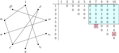
Figure 7: The random graph $G_{n,c/n}$ contains triangles when $c$ is large enough. The highlighted 0 bits in the last five rows can be deduced from pairs of 1 bits in the first 5 rows.

1. Event $\mathcal{E}_{1}$: The number $n_{1}(M)$ of ones in $M$ is at most $cn/8$. In this case, the number of ones in this submatrix is much less than the expected number, $cn/4$. We can simply apply Chernoff’s bound to show that $\Pr\left\{\mathcal{E}_{0}\right\}=2^{-\varOmega(c^{3})}$. We leave this as an exercise to the reader.

2. Event $\mathcal{E}_{2}$: Fix $n/2+1\leq j<k\leq n$, and let $\mathcal{B}_{jk}$ be the event that $M$ contains at least three rows $1\leq i_{1}<i_{2}<i_{3}\leq n/2$ with $A_{i_{l},j}=A_{i_{l},k}=1$, for $l=1,2,3$. Clearly, we have $\Pr\left\{\mathcal{B}_{jk}\right\}\leq\binom{n/2}{3}(c/n)^{6}=O\left(c^{6}/n^{3}\right)$. Let $\mathcal{E}_{2}$ be the event that $\mathcal{B}_{jk}$ holds for at least one pair $n/2+1\leq j<k\leq n$. Since there are $\binom{n/2}{2}$ such pairs, we have $\Pr\left\{\mathcal{E}_{2}\right\}=O(c^{6}/n)=2^{-\varOmega(c^{3})}$, as we assumed $c\leq\log^{1/3}n$.

3. Event $\mathcal{E}_{3}$: Let $\mathcal{E}_{3}$ be the event that (i) the number of ones in $M$ is greater than $cn/8$; (ii) for each pair $n/2+1\leq j<k\leq n$, there are at most two rows in $M$ where both the entry with index $j$ and the entry with index $k$ are set two one; and (iii) $G$ contains no triangles. Notice that, for $i<j<k$ if $A_{i,j}=1$ and $A_{i,k}=1$, then the fact that there are no triangles implies that $A_{j,k}=0$.

   Let $m_{i}$ be the number of ones in the $i$-th row of the submatrix. By specifying rows $1,\dots,n/2$, we eliminate the need to specify

   $$m\geq(1/2)\sum_{i=1}^{n/2}\binom{m_{i}}{2}\geq(n/4)\binom{2n_{1}(M)/n}{2}\geq(n/4)\binom{c/4}{2}=\varOmega(c^{2}n)\enspace,$$

   zeros in rows $n/2+1,\dots,n$ (here, we used the fact that each pair of ones appears in at most two rows and that the function $x\mapsto\binom{x}{2}$ is convex and increasing for $x\geq 1/4$). We thus encode $G$ by giving a Shannon-Fano code with parameter $p$ for the first $n/2$ rows of $A$; and a Shannon-Fano code with parameter $p$ for the rest of $A$, excluding the bits which can be deduced from the preceding information. Such a code has length

   $$|C(G)|=n_{1}(A)\log(1/p)+(n_{0}(A)-m)\log(1/(1-p))$$

   which results in a savings of

   $$s=\log(1/p_{G})-|C(G)|=m\log(1/(1-p))\geq\varOmega(c^{2}n)\log(1/(1-p))=\varOmega(c^{3})\enspace.$$

   It follows that $\Pr\left\{\mathcal{E}_{3}\right\}\leq 2^{-\varOmega(c^{3})}$.

Now the probability that $G$ contains no triangles is at most $\Pr\left\{\mathcal{E}_{1}\right\}+\Pr\left\{\mathcal{E}_{2}\right\}+\Pr\left\{\mathcal{E}_{3}\right\}=2^{-\varOmega(c^{3})}$. ∎

Theorem 18.

If $p=c/n$ with $c>0$, then $G\in G_{n,p}$ has no triangle with probability at least $1-c^{3}$.

Proof.

Suppose that $G$ contains a triangle. We encode the adjacency matrix $A$ of $G$. First, we specify the triangle’s vertices; and finish with a Shannon-Fano code with parameter $p$ for the remaining edges of the graph. This code has length

$$|C(G)| =3\log n+(n_{1}(A)-3)\log(1/p)+n_{0}(A)\log(1/(1-p))$$

$$=\log(1/p_{G})+3\log n-3\log(1/p)=\log(1/p_{G})+3\log c=\log(1/p_{G})+\log c^{3}\enspace.$$

∎

Together, Theorem 17 and Theorem 18 establish the fact that $1/n$ is a threshold function for triangle-freeness, i.e. if $p=o(1/n)$, then $G\in G_{n,p}$ has no triangle with high probability, and if $p=\omega(1/n)$, then $G$ has a triangle with high probability.

7 Encoding with Kraft’s Condition

As promised in Section 2.3, we finally discuss why it has made sense to omit ceilings in all of our encoding arguments.

Let $[0,\infty]$ denote the set of extended non-negative real numbers, supporting the extended arithmetic operations $a+\infty=\infty$ for all $a\in[0,\infty]$, and $2^{-\infty}=0$.

Recall from Section 5 that a function $\ell:X\to[0,\infty]$ satisfies Kraft’s condition if

$$\sum_{x\in X}2^{-\ell(x)}\leq 1\enspace.$$

The main observation is that neither the (Non-)Uniform Encoding Lemma nor any of its applications has actually required the specification of an explicit prefix-free code: We know, by construction, that every code we have presented is prefix-free, but we could also deduce from Kraft’s inequality that, since our described codes satisfy Kraft’s condition, a prefix-free code with the same codeword lengths exists. Similarly, we will see that it is actually enough to assign to every element from our universe a codeword length such that Kraft’s condition is satisfied. These codeword lengths need not be integers.

Lemma 9 (The encoding lemma for the Kraft inequality).

Let $\ell:X\to[0,\infty]$ satisfy Kraft’s condition and let $x\in X$ be drawn randomly where $p_{x}>0$ denotes the probability of drawing $x$. Then

$$\Pr\{\ell(x)\leq\log(1/p_{x})-s\}\leq 2^{-s}\enspace.$$

Proof.

The proof is identical to that of Lemma 8. ∎

The sum of two functions $\ell:X\to[0,\infty]$ and $\ell^{\prime}:X^{\prime}\to[0,\infty]$ is the function $\ell+\ell^{\prime}:X\times X^{\prime}\to[0,\infty]$ defined by $(\ell+\ell^{\prime})(x,x^{\prime})=\ell(x)+\ell^{\prime}(x^{\prime})$. Note that for any partial codes $C:X\nrightarrow\{0,1\}^{*},C^{\prime}:X^{\prime}\nrightarrow\{0,1\}^{*}$, any $x\in X$, and any $x^{\prime}\in X^{\prime}$,

$$(|C|+|C^{\prime}|)(x,x^{\prime})=|C(x)|+|C^{\prime}(x^{\prime})|=|(C\cdot C^{\prime})|(x,x^{\prime})\enspace.$$

In other words, the sum of the functions of codeword lengths describes the length of codewords in concatenated codes.

Lemma 10.

If $\ell:X\to[0,\infty]$ and $\ell^{\prime}:X^{\prime}\to[0,\infty]$ satisfy Kraft’s condition, then so does $\ell+\ell^{\prime}$.

Proof.

Kraft’s condition still holds:

$$\sum_{(x,x^{\prime})\in X\times X^{\prime}}2^{-(\ell+\ell^{\prime})(x,x^{\prime})}=\sum_{x\in X}\sum_{x^{\prime}\in X^{\prime}}2^{-\ell(x)-\ell^{\prime}(x^{\prime})}=\sum_{x\in X}2^{-\ell(x)}\sum_{x^{\prime}\in X^{\prime}}2^{-\ell^{\prime}(x^{\prime})}\leq 1\enspace.$$

∎

This is analogous to the fact that the concatenation of prefix-free codes is prefix-free.

Lemma 11.

For any probability density $p:X\to(0,1)$, the function $\ell:X\to[0,\infty]$ with $\ell(x)=\log(1/p_{x})$ satisfies Kraft’s condition.

Proof.

$$\sum_{x\in X}2^{-\ell(x)}=\sum_{x\in X}2^{-\log(1/p_{x})}=\sum_{x\in X}p_{x}=1\enspace.$$

∎

This tells us that we can ignore the ceiling in every instance of a fixed-length code and every instance of a Shannon-Fano code while encoding.

We now give a tight notion corresponding to Elias codes.

Theorem 19 (Beigel [5]).

Fix some $0<\varepsilon<e-1$. Let $\ell:\mathbb{N}\to\mathbb{R}$ be defined as

$$\ell(i)=\log i+\log\log i+\cdots+\underbrace{\log\cdots\log}_{\text{$\log^{*}i$ times}}i-(\log\log(e-\varepsilon))\log^{*}i+O(1)\enspace.$$

Then, $\ell$ satisfies Kraft’s condition. Moreover, the function $\ell^{\prime}:\mathbb{N}\to\mathbb{R}$ with

$$\ell^{\prime}(i)=\log i+\log\log i+\cdots+\underbrace{\log\cdots\log}_{\text{$\log^{*}i$ times}}i-(\log\log e)\log^{*}i+c$$

does not satisfy Kraft’s condition for any choice of the constant $c$.

It is not hard to see how Lemma 9, Lemma 10, Lemma 11, and Theorem 19 can be used to give encoding arguments with real-valued codeword lengths. For example, recall how the result of Theorem 1 carried an artifact of binary encoding. Using our new tools, we can now refine this and recover the exact result.

Theorem 1b.

Let $x=(x_{1},\ldots,x_{n})\in\{0,1\}^{n}$ be chosen uniformly at random and let $t={\lceil\log n+s\rceil}$. Then, the probability that $x$ contains a run of $t$ ones is at most $2^{-s}$.

Proof.

Let $\ell:\{0,1\}^{n}\to[0,\infty]$ be such that if $x$ contains a run of $t={\lceil\log n+s\rceil}$ ones, then $\ell(x)=\log n+n-t$, and otherwise $\ell(x)=\infty$. We will show that $\ell$ satisfies Kraft’s condition.

Let the function $f:\{1,\ldots,n-t+1\}\to[0,\infty]$ have $f(i)=\log n$ for all $i\in\{1,\dots,n-t+1\}$, and $g:\{0,1\}^{n-t}\to[0,\infty]$ have $g(y)=n-t$ for all $y\in\{0,1\}^{n-t}$. Both $f$ and $g$ satisfy Kraft’s condition by Lemma 11. By Lemma 10, so does the function

$$h=f+g:\{1,\ldots,n-t+1\}\times\{0,1\}^{n-t}\to[0,\infty]\enspace,$$

where $h(i,y)=\log n+n-t$ for all $i$ and $y$. Crucially, each element $(i,(y_{1},\dots,y_{n-1}))\in\{1,\ldots,n-t+1\}\times\{0,1\}^{n-t}$ yields to an $n$-bit binary string containing a run of $t$ ones, namely

$$(y_{1},\dots,y_{i-1},\underbrace{1,1,\dots,1}_{\text{$t$ times}},y_{i},\dots,y_{n-t})\enspace,$$

and this mapping is surjective. Thus, $\ell$ is as desired. We finish by applying Lemma 9. ∎

8 Summary and Conclusions

We have described a simple method for producing encoding arguments. Using our encoding lemmas, we gave original proofs for several previously established results.

Encoding arguments often give natural and short proofs for results in the analysis of algorithms, particularly for algorithms which directly handle bit strings. Many of our results concern the worst-case running time of algorithms, but encoding arguments can also be used to study other measures of algorithmic complexity, such as the average-case running time of algorithms, or the communication complexity of Boolean functions [8].

Typically, to produce an encoding argument, one would invoke the incompressibility method after developing some of the theory of Kolmogorov complexity. Our technique requires only a basic understanding of prefix-free codes and one simple lemma. We are also the first to suggest a simple and tight manner of encoding using only Kraft’s condition with real-valued codeword lengths. In this light, we posit that there is no reason to develop an encoding argument through the incompressibility method: our Uniform Encoding Lemma is simpler, the Non-Uniform Encoding Lemma is more general, and our technique from Section 7 is less wasteful. Indeed, though it would be easy to state and prove our Non-Uniform Encoding Lemma in the setting of Kolmogorov complexity, it seems as if the general encoding lemma from Section 7 only can exist in our simplified framework.

References

- [1] ACM/IEEE-CS Joint Task Force on Computing Curricula. Computer science curricula 2013: Curriculum guidelines for undergraduate degree programs in computer science. Technical report, ACM Press and IEEE Computer Society Press, December 2013.
- [2] N. Alon and J. H. Spencer. The Probabilistic Method. Wiley Series in Discrete Mathematics and Optimization. Wiley-Interscience, 4 edition, 2016.
- [3] Y. Azar, A. Z. Broder, A. R. Karlin, and E. Upfal. Balanced allocations. SIAM Journal on Computing, 29(1):180–200, February 2000.
- [4] A. R. Barron. Logically Smooth Density Estimation. PhD thesis, Stanford University, September 1985.
- [5] R. Beigel. Unbounded searching algorithms. SIAM Journal on Computing, 19(3):522–537, 1990.
- [6] P. Berenbrink, A. Czumaj, A. Steger, and B. Vöcking. Balanced allocations: The heavily loaded case. SIAM Journal on Computing, 35(6):1350–1385, 2006.
- [7] R. Boucheron, G. Lugosi, and P. Massart. Concentration Inequalities: A Nonasymptotic Theory of Independence. Oxford University Press, Oxford, United Kingdom, 2013.
- [8] H. Buhrman, T. Jiang, M. Li, and P. Vitányi. New applications of the incompressibility method: Part II. Theoretical Computer Science, 235(1):59–70, 2000.
- [9] A. Cayley. A theorem on trees. Quarterly Journal of Mathematics, 23:376–378, 1889.
- [10] H. Chernoff. A measure of asymptotic efficiency for tests of a hypothesis based on the sum of observations. The Annals of Mathematical Statistics, 23(4):493–507, 12 1952.
- [11] L. Devroye. Applications of the theory of records in the study of random trees. Acta Informatica, 26(1):123–130, 1988.
- [12] L. Devroye, P. Morin, and A. Viola. On worst-case Robin Hood hashing. SIAM Journal on Computing, 33(4):923–936, 2004.
- [13] D. P. Dubhashi and A. Panconesi. Concentration of Measure for the Analysis of Randomized Algorithms. Cambridge University Press, New York, New York, 2009.
- [14] P. Elias. Universal codeword sets and representations of the integers. IEEE Transactions on Information Theory, 21(2):194–203, March 1975.
- [15] P. Erdős. Some remarks on the theory of graphs. Bulletin of the American Mathematics Society, 53:292–294, 1947.
- [16] P. Erdős and L. Lovász. Problems and results on 3-chromatic hypergraphs and some related questions. In A. Hajnal, R. Rado, and V. T. Sós, editors, Infinite and Finite Sets, volume 10 of Colloquia Mathematica Societatis János Bolyai, pages 609–627. North-Holland, 1973.
- [17] R. M. Fano. The transmission of information. Technical Report 65, Research Laboratory of Electronics at MIT, Cambridge, Massachusetts, 1949.
- [18] L. Fortnow. A Kolmogorov complexity proof of the Lovász local lemma. http://blog.computationalcomplexity.org/2009/06/kolmogorov-complexity-proof-of-lov.html, 2009. (last accessed November 28, 2015).
- [19] G. R. Grimmett. Percolation. 321. Springer-Verlag Berlin Heidelberg, 2 edition, 1999.
- [20] T. Haimberger. Theoretische und Experimentelle Untersuchung von Kuckucks-Hashing. Bachelor’s thesis. Freie Universität Berlin, 2013.
- [21] C. A. R. Hoare. Algorithm 65: Find. Communications of the ACM, 4(7):321–322, July 1961.
- [22] S. Hoory, N. Linial, and A. Wigderson. Expander graphs and their applications. Bulletin of the American Mathematical Society, 43(4):439–561, October 2006.
- [23] B. Lucier, T. Jiang, and M. Li. Average-case analysis of Quicksort and binary insertion tree height using incompressibility. Information Processing Letters, 103(2):45–51, July 2007.
- [24] C. McDiarmid. On the method of bounded differences. In J. Siemons, editor, Surveys in Combinatorics: Invited Papers at the 12th British Combinatorial Conference, number 141, pages 148–188. Cambridge University Press, 1989.
- [25] J. Messner and T. Thierauf. A Kolmogorov complexity proof of the Lovász local lemma for satisfiability. Theoretical Computer Science, 461:55–64, November 2012.
- [26] M. Mitzenmacher and E. Upfal. Probability and Computing: Randomized Algorithms and Probabilistic Analysis. Cambridge University Press, 2005.
- [27] P. Morin. Open Data Structures: An Introduction. Athabasca University Press, Edmonton, 2013. Also freely available at opendatastructures.org.
- [28] R. A. Moser. A constructive proof of the Lovász local lemma. In Proceedings of the 41st Annual ACM Symposium on Theory of Computing, STOC ’09, pages 343–350, New York, NY, USA, 2009. ACM.
- [29] R. A. Moser and G. Tardos. A constructive proof of the general Lovász local lemma. Journal of the ACM, 57(2):11:1–11:15, January 2010.
- [30] R. Motwani and P. Raghavan. Randomized Algorithms. Cambridge University Press, New York, New York, 1995.
- [31] R. Pagh and F. F. Rodler. Cuckoo hashing. Journal of Algorithms, 51(2):122–144, 2004.
- [32] M. S. Pinsker. On the complexity of a concentrator. In The 7th International Teletraffic Conference, volume 4, pages 1–4, 1973.
- [33] M. Pătraşcu. Cuckoo hashing. http://infoweekly.blogspot.ca/2010/02/cuckoo-hashing.html, 2010. (last accessed April 15, 2015).
- [34] B. Reed. The height of a random binary search tree. Journal of the ACM, 50(3):306–332, May 2003.
- [35] H. Robbins. A remark on Stirling’s formula. The American Mathematical Monthly, 62(1):26–29, jan 1955.
- [36] R. Sedgewick and P. Flajolet. An Introduction to the Analysis of Algorithms. Addison-Wesley Longman Publishing Co., Inc., Boston, MA, USA, 1996.
- [37] C. E. Shannon. A mathematical theory of communication. Bell Systems Technical Journal, 27:379–423, 1948.
- [38] P. Vitányi. Analysis of sorting algorithms by Kolmogorov complexity (a survey). In Entropy, Search, Complexity, volume 16 of Bolyai Society Mathematical Studies, pages 209–232. Springer-Verlag New York, 2007.
- [39] B. Vöcking. How asymmetry helps load balancing. Journal of the ACM, 50(4):568–589, July 2003.