Dynamics of Modified Chaplygin Gas Inflation on the Brane with Bulk Viscous Pressure

Abstract

We investigate the role of bulk viscous pressure on the warm inflationary modified Chaplygin gas in brane-world framework in the presence of standard scalar field. We assume the intermediate inflationary scenario in strong dissipative regime and constructed the inflaton, potential, entropy density, slow-roll parameters, scalar and tensor power spectra, scalar spectral index and tensor-to-scalar ratio. We develop various trajectories such as $n_{s}-N$, $n_{s}-r$ and $n_{s}-\alpha_{s}$ (where $n_{s}$ is the spectral index, $\alpha_{s}$ is the running of spectral index, $N$ is the number of e-folds and $r$ is tensor-to-scalar ratio) for variable as well as constant dissipation and bulk viscous coefficients at high dissipative regime. It is interesting to remark here that our results of these parameters are compatible with recent observational data such as WMAP $7+9$, BICEP$2$ and Planck data.

Keywords: Braneworld model; Warm intermediate inflation; Modified
Chaplygin gas model ; Inflationary parameters.

1 Introduction

At early times, there was a segment in which the universe evolved through accelerated expansion in a short period of time at high energy scales which result the idea of inflation. Inflationary theory has major achievements in solving the longstanding cosmological puzzles like monopole, flatness, horizon etc [1, 2]. The mechanism of large-scale structure (LSS) and anisotropy of cosmological microwave background (CMB) is explained by inflationary theory [3, 4]. In warm inflationary models, the radiation production arises during inflationary period and reheating can be avoided [5]. The thermal fluctuations could be obtain in these models which produce initial fluctuations and are crucial for LSS formation. Warm inflationary period ends when the universe stops inflating and after that, the universe enters in radiation phase smoothly [5]. In the end, remaining inflatons or dominant radiation fields produced the matter components of the universe. For the sake of simplicity, the particles (which are produced due to inflaton decay) are assumed as massless particles (or radiation) in warm inflation models.

The existence of massive particles has been considered in [6] and corresponding perturbation parameters of this model have been presented in [7]. Decay of the massive particles within the fluid is an entropy-producing scalar phenomenon, on the other hand bulk viscous pressure has entropy-producing property. Therefore the decay of particles may be assumed as a bulk viscous pressure $\Pi=-3\xi H$ [8], where $H$ and $\xi$ are Hubble parameter and phenomenological coefficient of bulk viscosity, respectively. This coefficient is positive-definite by the second law of thermodynamics and depends on the energy density of the fluid. The inflationary epoch can be divided into epochs such as slow-roll and reheating. During the slow-roll approximation, the universe inflates as the interactions between inflatons and other fields become negligibly small and the potential energy dominates the kinetic energy. After this period, the universe enters the last stage of inflation, i.e., the reheating era, in which the kinetic and potential energies are comparable. Here the inflation starts to oscillate around the minimum of its potential while losing its energy to massless particles. During inflationary phase, the forms of energy density like radiation or matter were dominated by the vacuum energy while the scale factor increased exponentially over time [9].

The cosmic acceleration in the early universe (or inflationary universe) can be realized by a scalar field (inflaton) through an effective potential which represents the evolution of this field. The scalar field models deal with two pictures of inflation, i.e., slow-roll and reheating. During the slow-roll phase, the universe undergoes a rapid expansion while kinetic term of inflaton is less than that of potential energy. In the reheating period, these two energies are comparable and inflaton starts to oscillate about the minimum of the potential by loosing its energy to other radiation fields [10]. Moreover, MCG explains the expansion of the universe from phase dominated for small values of cosmological scale factor using EoS i.e, $p=\omega\rho$ to large values of scale factor using cosmological constant i.e, $(\frac{\beta}{1+\omega})^{\frac{1}{1+n}}$ [11]. A fluid of (modified) CG is usually applied to explain the late time acceleration of our universe as a possible candidate of dark energy. MCG mimics the behavior of matter at early-times and that of a cosmological constant at late-times. CMB also indicated that the early universe also passes through an accelerating phase too, which is the inflationary epoch. Given the attractiveness of the MCG as a dark energy candidate, a natural question to ask is: Can inflation be accommodated within the MCG scenario? This is the question we wish to address in the present work. However, we should emphasize that our inflationary model is not presented as a more desirable alternative to the conventional ones. Rather, we merely aim to establish the assumptions and extrapolations required to obtain successful inflation in a Chaplygin inspired model [12].

A feasible solution called intermediate inflation scenario exists in the literature which is defined as $a=\exp(At^{f})$, where $f$ is constant ($0<f<1$). In this scenario, the expansion of the universe is slower than standard de Sitter inflation $(a=e^{Ht})$ while faster than power law inflation $(a=t^{p},~{}p>1)$. This method was introduced for a particular scalar field potential of the type $V(\phi)\propto\phi^{-4(f^{-1}-1)}$ as the universe was controlled by a potential $V(\phi)$ during inflationary period [13, 14]. In the slow-roll estimation with this type of potential, it is possible to have a spectrum of density perturbations which presents a scale invariant spectral index, i.e. $n_{s}=1$.

Yokoyama and Maeda [15] worked on intermediate inflation in the brane-world scenario and demonstrated the nonzero value of tensor-scalar ratio. Bamba et al. [16] have considered inflationary cosmology in a viscous fluid model. Setare and Kamali [17] investigated warm-viscous inflation on the brane by taking chaotic potential and found that the values of all involved parameters are consistent with Wilkinson Microwave Anisotropy Probe (WMAP)$9$, Planck and BICEP$2$ observational data. Herrera and Campo [18] examined the parameters slow-roll parameters, inflaton, energy density, entropy density, etc on the brane intermediate inflationary model in high dissipative regime and found the consistency with WMAP$5$. Setare and Kamali [19] worked on the brane with warm-viscous inflationary universe model and tachyon scalar field. They have calculated the parameters of this inflationary model which are compatible with WMAP$7$. Setare and Kamali [20] studied the tachyon-warm intermediate and logamediate inflation in the brane-world scenario by taking exponential potential and compared their results with recent observational data from WMAP$9$ and Planck data.

In the present work, we investigate the inflationary parameters for warm intermediate inflation with bulk viscous pressure in high dissipative scenario. The outline of the paper is as follows: Basic equations related to braneworld model and Chaplygin gas (CG) models are discussed in section 2. In section 3, we will consider different characteristics of warm intermediate inflation and examine the results of slow$-$roll parameters according to braneworld model along with modified Chaplygin gas (MCG). Detailed discussions of perturbed parameters for variable coefficients as well as constant coefficients will take place in section 4. Section 5 contains the conclusion.

2 Braneworld Model

In the braneworld scheme, the observable four-dimensional universe is considered as a domain wall implanted on a higher-dimensional bulk space. Einstein s field equation in the braneworld theory with cosmological constant as a matter and source fields bounded to 3-brane may be designed as follows [21]

$$G_{\mu\nu}=-\Lambda_{4}g_{\mu\nu}+\bigg{(}\frac{8\pi}{M_{4}^{2}}\bigg{)}T_{\mu\nu}+\bigg{(}\frac{8\pi}{M_{5}^{2}}\bigg{)}^{2}\pi_{\mu\nu}-E_{\mu\nu},$$

where $E_{\mu\nu}$ is a projection of $5$d Weyl tensor, $M_{4}$ and $M_{5}$ are Planck scales in $4$ and $5$ dimensions respectively, $T_{\mu\nu}$ is energy density tensor on the brane and $\pi_{\mu\nu}$ is a tensor quadratic in $T_{\mu\nu}$. Effectual cosmological constant $\Lambda_{4}$ on the brane in terms of 3-brane tension $\sigma$ and cosmological constant ($\Lambda$) is given by

$$\Lambda_{4}=\frac{4\pi}{M_{5}^{3}}\bigg{(}\Lambda+\frac{4\pi}{3M_{5}^{3}}\sigma^{2}\bigg{)},$$

and $4$d Planck scale is determined by $5$d Planck scale as

$$M_{4}=\bigg{(}\frac{3}{4\pi}\bigg{)}^{\frac{1}{2}}\bigg{(}\frac{M_{5}^{2}}{\sqrt{\sigma}}\bigg{)}M_{5}.$$

The spatially flat FRW space comprised by line element as follows

$$ds^{2}=-dt^{2}+a^{2}(t)(dx^{2}+dy^{2}+dz^{2})$$

where $a(t)$ is the scale factor. For flat FRW model, Friedmann equation on the brane turns out to be [21]

$$H^{2}=\frac{\Lambda_{4}}{3}+\bigg{(}\frac{8\pi}{3M_{4}^{2}}\bigg{)}\rho_{\tau}+\bigg{(}\frac{4\pi}{3M_{5}^{2}}\bigg{)}\rho_{\tau}^{2}+\frac{\varepsilon}{a^{4}},$$

where $\rho_{\tau}$ is total energy density on the brane. In the above equation, last term denotes the shape of the bulk gravitons on the brane, where $\varepsilon$ is an integration constant which comes up from Weyl tensor $E_{\mu\nu}$. The projected Weyl tensor term in the effectual Einstein equation may be neglected because this term may be speedily stretched when the inflation starts [19]. It is also assumed that the $\Lambda_{4}$ is negligible in the early universe. The Friedmann equation is reduced to

$$H^{2}=\frac{8\pi}{3M_{4}^{2}}\rho_{\tau}\bigg{(}1+\frac{\rho_{\tau}}{2\lambda}\bigg{)}.$$

The equation of state of pure CG is defined as

$$p=-\frac{\beta}{\rho},$$

where $\beta$ is positive parameter, $p$ represents pressure and $\rho$ is the energy density. The extended form of CG was driven by Kamenshchik et al. [22], named as generalized CG (GCG) is given by

$$p=-\frac{\beta}{{\rho}^{\sigma}},\quad 0<\sigma<1.$$

An advance study of CG called MCG has been introduced by Benaoum [23, 24] with the following equation of state

$$p_{MCG}=\omega\rho_{MCG}-\frac{\beta}{{\rho_{MCG}}^{\sigma}},\quad 0<\sigma<1$$

where $\omega$ is a positive constant. The energy conservation equation for MCG model described as:

$$\rho_{MCG}=\bigg{(}\frac{\beta}{1+\omega}+\frac{\upsilon}{a^{3(1+\sigma)(1+\omega)}}\bigg{)}^{\frac{1}{1+\sigma}},$$

where $\upsilon$ is constant of integration.

3 Basic Inflationary Scenario

Now we study different characteristics of intermediate inflationary MCG model for FRW universe distinguished by inflaton and matter radiation. By assuming perturbed parameters, we fix our model everywhere at intermediate epoch and assure the compatibility with observational data. The warm MCG model including imperfect fluid on the brane modifies first Friedmann equation as [25]

$$H^{2} = \frac{8\pi}{3M_{4}^{2}}\bigg{(}\rho_{\phi}+\rho\bigg{)}\bigg{(}1+\frac{\rho_{\phi}+\rho}{2\lambda}\bigg{)}$$ (1)

$$= \frac{8\pi}{6M_{4}^{2}\lambda}\bigg{[}\bigg{(}\frac{\beta}{1+\omega}+\upsilon\rho_{\phi}^{(1+\sigma)(1+\omega)}\bigg{)}^{\frac{1}{1+\sigma}}+TS(\phi,T)\bigg{]}\bigg{[}2\lambda+\bigg{(}\frac{\beta}{1+\omega}$$

$$+ \upsilon\rho_{\phi}^{(1+\sigma)(1+\omega)}\bigg{)}^{\frac{1}{1+\sigma}}+TS(\phi,T)\bigg{]},$$

where we have used $\rho_{\tau}=\rho_{\phi}+\rho$ and $\rho$ is taking as energy density in terms of imperfect fluid $\rho=TS(\phi,T)$ ($T$ represents temperature and $S$ stands for entropy density). Also, $\rho_{\phi}$ is assumed to be the energy density of MCG.

Since $\rho_{\phi}\ll\rho_{\phi}^{2}$, then Eq.(1) leads to [18]

$$H^{2} = \frac{8\pi}{6M_{4}^{2}\lambda}\bigg{[}\bigg{(}\frac{\beta}{1+\omega}+\upsilon\rho_{\phi}^{(1+\sigma)(1+\omega)}\bigg{)}^{\frac{1}{1+\sigma}}+TS(\phi,T)\bigg{]}^{2}.$$

The most important parameters of inflation are energy density $\rho_{\phi}$ and pressure $p_{\phi}$ which can be defined as follows

$$\rho_{\phi}=\frac{\dot{\phi}^{2}}{2}+V(\phi),\quad p_{\phi}=\frac{\dot{\phi}^{2}}{2}-V(\phi),$$

where dot denotes derivative with respect to time $t$ and $V(\phi)$ is used as potential term.

The inflaton and imperfect fluid energy densities are conserved as

$$\dot{\rho}+3H(\psi\rho+\Pi)=\Gamma\dot{\phi}^{2}.$$ (2)

$$\dot{\rho_{\phi}}+3H(\rho_{\phi}+p_{\phi})=-\Gamma\dot{\phi}^{2}.$$ (3)

Here, we have used the bulk viscous pressure defined as as $p+\Pi$, while $p=(\psi-1)\rho$ with adiabatic index $1\leq\psi\leq 2$ and $\Pi=-3\xi H$ is bulk viscous pressure ($\xi$ is the coefficient of bulk viscosity which is positive-definite and generally depends on $\rho$). Also $\Gamma$ is the dissipation factor that assess the rate of decay of $\rho_{\phi}$ into $\rho$. The second law of thermodynamics indicates that $\Gamma$ must be positive, so the inflaton energy density decompose into radiation density. Energy density of imperfect fluid is $\rho=TS(\phi,T)$ which changes the Eq.(2) as

$$S\dot{T}+T\dot{S}+3H(\psi TS+\Pi)=\Gamma\dot{\phi}^{2},$$

here, $\dot{T}$ is negligible. The negativity of bulk viscous pressure contributes to increase the source of entropy density given on the right-hand side of the above equation. The second conservation equation can be written in view of $\rho_{\phi}$ and $p_{\phi}$ as

$$\ddot{\phi}+(3H+\Gamma)\dot{\phi}+\acute{V(\phi)}=0\Rightarrow\ddot{\phi}+3H(1+\frac{\Gamma}{3H})\dot{\phi}+\acute{V(\phi)}=0$$

where $\frac{\Gamma}{3H}=R$ and prime represents the derivative with respect to $\phi$. In weak dissipative epoch, $R\ll 1$ runs to $\Gamma\ll 3H$ while $R\gg 1$ denotes high dissipative era (where dissipation coefficient is much bigger than Hubble scale). The evolution of the universe during inflationary regime diffuses the decay of inflaton for $R\ll 1$. Bulk viscosity cannot be neglected when the sectors of the inflationary fluid interact with each other and turns negligible throughout this region. Implementation of limits required for getting the epoch to be static, i.e. $\rho_{\phi}\approx V(\phi),\rho<\rho_{\phi}$, slow-roll limit, $V(\phi)\gg\dot{\phi}^{2}$, $(3H+\Gamma)\dot{\phi}\gg\ddot{\phi}$ and quasi-stable decay of $\rho_{\phi}$ into $\rho$, where $3H(\psi\rho+\Pi)\gg\dot{\rho}$, $\Gamma\dot{\phi}^{2}\gg\dot{\rho}$. When all these limits apply in the Eqs.(2) and (3) then dynamical equations takes the form as

$$H^{2} = \frac{8\pi}{6M_{4}^{2}\lambda}\bigg{(}\frac{\beta}{1+\omega}+\upsilon\rho_{\phi}^{(1+\sigma)(1+\omega)}\bigg{)}^{\frac{2}{1+\sigma}},$$ (4)

$$\dot{\phi} = \frac{-V^{\prime}(\phi)}{3H(1+r)},$$ (5)

$$\psi\rho = r\dot{\phi}^{2}-\Pi.$$ (6)

The essential slow-roll approximation is controlled by a set of dimensionless slow-roll parameters which are defined as [26]

$$\epsilon=-\frac{\dot{H}}{H^{2}},~{}~{}~{}~{}~{}~{}~{}~{}~{}~{}~{}~{}\eta=-\frac{\ddot{H}}{H\dot{H}}.$$

These parameters for inflationary viscous universe model can be represented as

$$\epsilon = \left(\frac{3\lambda M_{4}^{2}}{4\pi}\right)^{2}\frac{\upsilon(1+\omega)V^{-1+(1+\sigma)(1+\omega)}V^{\prime 2}}{R\left(\frac{\beta}{1+\omega}+\upsilon V^{(1+\sigma)(1+\omega)}\right)^{1+\frac{4}{1+\sigma}}}.$$ (7)

$$\eta = 3\lambda M_{4}^{2}\left(\beta(\sigma+\omega+\sigma\omega)-\upsilon(1+\omega)V^{(1+\sigma)(1+\omega)}\right)V^{\prime 2}+2V\bigg{(}\beta+\upsilon(1+\omega)$$ (8)

$$\times V^{(1+\sigma)(1+\omega)}\bigg{)}V^{\prime\prime}\bigg{[}12\pi(1+R)V\left(\beta+\upsilon(1+\omega)V^{(1+\sigma)(1+\omega)}\right)\bigg{(}\frac{\beta}{1+\omega}+\upsilon$$

$$\times V^{(1+\sigma)(1+\omega)}\bigg{)}^{\frac{2}{1+\sigma}}\bigg{]}^{-1}.$$

These parameters are smaller than $1+R$ lead to the sensible slow-roll limit. The condition $\epsilon<1$ leads to $\rho_{\phi}>3(1+\omega)(\psi\rho+\Pi)^{1-(1+\sigma)(1+\omega)}$. The slow-roll inflation ends at $\epsilon=1$. The inflation not only demands $\epsilon<1$ but also $\eta$ must be small over a reasonably large period of time, enough number of e-folds represented by $N$. We bound our model in the region $\phi>0$. This number can be calculated by using the following formula

$$N(\phi) = \int^{t_{g}}_{t_{i}}Hdt=\int^{\phi_{g}}_{\phi_{i}}(4\pi R)(V^{\prime}\lambda M_{4}^{2})^{-1}\bigg{(}\frac{\beta}{1+\omega}+\upsilon V^{(1+\sigma)(1+\omega)}\bigg{)}^{\frac{2}{1+\sigma}}$$ (9)

where $\phi_{i}$ and $\phi_{g}$ stand for initial and final inflatons respectively.

Also, Eq.(6) and slow-roll parameter ($\epsilon$) provides the following relationship between $\rho_{\phi}$ and $\rho$ including the effect of viscous pressure as

$$\psi\rho+\Pi = \bigg{[}\epsilon\bigg{(}2\lambda+\bigg{(}\frac{\beta}{1+\omega}+\upsilon\rho_{\phi}^{(1+\sigma)(1+\omega)}\bigg{)}^{\frac{1}{1+\sigma}}\bigg{)}\bigg{(}\frac{\beta}{1+\omega}+\upsilon\rho_{\phi}^{(1+\sigma)(1+\omega)}\bigg{)}$$

$$\times \rho_{\phi}^{1-(1+\sigma)(1+\omega)}\bigg{]}\bigg{[}3\upsilon(1+\omega)\bigg{(}\lambda+\bigg{(}\frac{\beta}{1+\omega}+\upsilon\rho_{\phi}^{(1+\sigma)(1+\omega)}\bigg{)}^{\frac{1}{1+\sigma}}\bigg{)}\bigg{]}^{-1}.$$

4 Perturbations

We consider different types of perturbations for FRW background and measure tensor and scalar disorders at minor stage by changing the value of $\phi$. There are basically four quantities which are mostly analyzed for inflationary disorders, i.e., tensor and scalar power spectra $(P_{r},P_{s})$, tensor and scalar spectral indices $(n_{r},n_{s})$. The form of scalar power spectrum can be estimated as $P_{r}(k_{0})\equiv\frac{25}{4}\delta_{H}^{2}(k_{0})$, where $K_{F}=\sqrt{\Gamma H}$ and density disorders $\delta_{H}^{2}(k_{0})\equiv\frac{K_{F}(T_{r})}{2\pi^{2}}$. We analyze the change in value of inflationary parameters by considering two different cases, i.e., (i) taking bulk and dissipation coefficients as variables (ii) taking bulk and dissipation coefficients as constants.

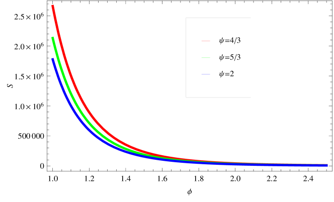
Figure 1: Plot of entropy density ($S(\phi)$) versus scalar field for $\lambda=1,~{}\sigma=1,~{}A=1,~{}M_{4}=1,~{}f=\frac{3}{5},~{}\Gamma=0.275,~{}\xi_{1}=0.2\times 10^{-8},~{}T=5.47\times 10^{-5},~{}\omega=0.25,~{}\beta=0.775,~{}\upsilon=1$.

4.1 Variable Bulk and Dissipative Coefficients

Here, we choose $\Gamma=\Gamma(\phi)=V(\phi)$ and $\xi=\xi(\rho)=\xi_{1}\rho$. With these constraints, inflaton and effective potential can be obtained by using Eqs.(4)-(5)

$$\phi-\phi_{0} = 2(1+b)t^{\frac{1}{2}(1+b)}(\upsilon(1+\omega))^{\frac{1}{2}}(f-1)^{\frac{-1}{2}}.$$

$$V(\phi) = \frac{3(Af)^{2}M_{4}^{2}\lambda}{4\pi}\bigg{[}(\upsilon(1+\omega))^{\frac{-1}{2}}(f-1)^{\frac{1}{2}}(2+2b)^{-1}\bigg{]}^{\frac{4(f-1)}{1+b}}\phi^{\frac{4(f-1)}{1+b}}.$$ (10)

respectively, and $b=(f-1)(1+\sigma)$. By using Eqs.(5)-(6), the entropy density leads to

$$S(\phi) = \frac{16Afb_{1}^{2}\bigg{(}\frac{1}{2(1+b)}\bigg{)}^{2b_{1}}\bigg{(}\frac{f-1}{\upsilon(1+\omega)}\bigg{)}^{2b_{1}}\phi^{-2+2b_{1}}}{T\psi\bigg{(}1-3A\xi_{1}\bigg{(}\frac{1}{2(1+b)}\bigg{)}^{2b_{1}}\bigg{(}\frac{f-1}{\upsilon(1+\omega)}\bigg{)}^{2b_{1}}\phi^{2b_{1}}\bigg{)}}.$$

where $b_{1}=\frac{f-1}{1+b}$. We plot $S(\phi)$ versus $\phi$ in Figure 1 and observe that it shows the increasing behavior of entropy density with respect to $\phi$ for three different values of $\psi$. There is no change in present model with and without bulk viscous pressure $\Pi$.

However, the slow roll parameter $\epsilon$ in terms of $\phi$ by using Eq. (7) turns out to be

$$\epsilon = \frac{1-f}{Af}\bigg{[}\phi^{\frac{2}{1+b}}(\upsilon(1+\omega))^{\frac{-1}{2}}(f-1)^{\frac{1}{2}}(2+2b)^{-1}\bigg{]}^{-f}$$ (11)

By setting $\epsilon=1$, we can get the value of lower bound on inflatons (defined as $\phi_{i}$) as follows

$$\phi_{i} = 2(1+b)\bigg{(}\frac{1-f}{Af}\bigg{)}^{\frac{1+b}{2f}}\bigg{(}\frac{\upsilon(1+\omega)}{f-1}\bigg{)}^{\frac{1}{2}}.$$

This lower bound of inflatons helps us in finding its upper bound in terms of number of e-folds ($N$) by taking Eq. (9) which is given by

$$\phi_{f}=(2(1+b))\bigg{(}\frac{\upsilon(1+\omega)}{f-1}\bigg{)}^{\frac{1}{2}}\bigg{[}\frac{N}{A}+\bigg{(}\frac{1-f}{Af}\bigg{)}\bigg{]}^{\frac{1+b}{2f}}.$$ (12)

The scalar power spectrum ($P_{r}$) in high dissipative era and amplitude of tensor perturbations $(A_{g}^{2})$ are computed by using the following formulae

$$P_{r}=\frac{T_{r}}{2\pi^{2}\epsilon\sqrt{RV^{3}}}\exp(-2\chi(\phi)),\quad A_{g}^{2}=2\bigg{(}\frac{H}{2\pi}\bigg{)}^{2}\coth\bigg{[}\frac{K}{2T}\bigg{]},$$

respectively. Here $T_{r}$ and $T$ are temperatures of air current fluctuations and thermal background of gravitational waves, respectively. Stimulated emissions rise up in the thermal background of gravitational waves during the multiplication of tensor perturbation in inflation. Therefore, the temperature of thermal background of gravitational waves has got an extra factor $\coth(\frac{K}{2T})$, where $K$ is the wave number. Further, $\chi(\phi)$ (an auxiliary function) in high dissipative regime can be defined as follows [27]

$$\chi(\phi)=-\int\bigg{\{}\frac{\Gamma^{\prime}}{3HR}+\frac{3}{8}\bigg{[}1-\bigg{(}(\psi-1)+\frac{\Pi}{\xi}\frac{d\xi}{d\rho}\bigg{)}\frac{\Gamma^{\prime}V^{\prime}}{9R\psi H^{2}}\bigg{]}\frac{V^{\prime}}{V}\bigg{\}}d\phi.$$ (13)

By using Eqs.(4), (10) in Eq.(13), $\chi$ takes the form

$$\chi(\phi) = -\frac{11}{8}\ln\phi+\frac{3(Af)}{16\psi}\bigg{(}\frac{1}{2(1+b)}\bigg{)}^{2b_{1}}\bigg{(}\frac{f-1}{\upsilon(1+\omega)}\bigg{)}^{b_{1}}\phi^{2(b_{1}-1)}$$ (14)

$$\times \bigg{[}\bigg{(}\frac{f-1}{\upsilon(1+\omega)}\bigg{)}^{b_{1}}\bigg{(}\frac{4b_{1}(\psi-1)}{b_{1}-1}\bigg{)}-\bigg{(}\frac{M_{4}^{2}Af\lambda}{4\pi}\bigg{)}\bigg{(}\frac{1}{2(1+b)}\bigg{)}^{2b_{1}}$$

$$\times \bigg{(}\frac{\xi_{1}}{2b_{1}-1}\bigg{)}\phi^{2b_{1}}\bigg{]}$$

The scalar power spectrum ($P_{r}$) and amplitude of tensor perturbations $(A_{g}^{2})$ in high dissipation epoch can be obtained by substituting the expressions (10), (11), (14) as

$$P_{r} = \frac{T_{r}\sqrt{3Af}}{2\pi^{2}}\bigg{(}\frac{4\pi}{3M_{4}^{2}(Af)^{2}\lambda}\bigg{)}^{2}\bigg{(}\frac{Af}{1-f}\bigg{)}\bigg{(}\frac{f-1}{\upsilon(1+\omega)}\bigg{)}^{\frac{7-5f}{2(1+b)}}\bigg{(}\frac{1}{2(1+b)}\bigg{)}^{\frac{7-5f}{1+b}}$$

$$\times \phi^{\frac{7-5f}{1+b}}\exp\bigg{[}\frac{11}{4}\ln\phi-\frac{3(Af)}{4\psi}\bigg{(}\frac{1}{2(1+b)}\bigg{)}^{2b_{1}}\bigg{(}\frac{f-1}{\upsilon(1+\omega)}\bigg{)}^{b_{1}}\phi^{2(b_{1}-1)}$$

$$\times \bigg{[}\bigg{(}\frac{f-1}{\upsilon(1+\omega)}\bigg{)}^{b_{1}}\bigg{(}\frac{4b_{1}(\psi-1)}{b_{1}-1}\bigg{)}-\bigg{(}\frac{M_{4}^{2}Af\lambda}{4\pi}\bigg{)}\bigg{(}\frac{1}{2(1+b)}\bigg{)}^{2b_{1}}$$

$$\times \bigg{(}\frac{\xi_{1}}{2b_{1}-1}\bigg{)}\phi^{2b_{1}}\bigg{]}\bigg{]},$$

$$A_{g}^{2} = \frac{(Af)^{2}}{2\pi^{2}}\bigg{(}\frac{1}{2(1+b)}\bigg{)}^{\frac{4(f-1)}{1+b}}\bigg{(}\frac{f-1}{\upsilon(1+\omega)}\bigg{)}^{\frac{4(f-1)}{1+b}}\coth\bigg{[}\frac{K}{2T}\bigg{]}_{K=K_{0}}\phi^{\frac{4(f-1)}{1+b}}.$$

Moreover, the ratios of factors $P_{r}$ to $A_{g}^{2}$ in high dissipative regime called the tensor-to-scalar ratio which is given by

$$r(K_{0})=\frac{P_{r}}{A_{g}^{2}}=\frac{2}{3}\bigg{[}\frac{\epsilon\sqrt{RV^{5}}}{T_{r}}\bigg{]}exp(2\chi(\phi))\coth\bigg{[}\frac{K}{2T}\bigg{]}_{K=K_{0}}$$

where $K_{0}=0.002Mpc^{-1}$ is the pivot point. The computation of this ratio for the present scenario turns out to be

$$r(K_{0}) = \frac{(1-f)\sqrt{Af}}{T_{r}\sqrt{3}}\bigg{(}\frac{f-1}{\upsilon(1+\omega)}\bigg{)}^{\frac{13f-15}{1+b}}\bigg{(}\frac{1}{2(1+b)}\bigg{)}^{\frac{9f-11}{1+b}}\bigg{(}\frac{3M_{4}^{2}(Af)^{2}\lambda}{4\pi}\bigg{)}^{2}$$

$$\times \coth\bigg{[}\frac{K}{2T}\bigg{]}_{K=K_{0}}\phi^{\frac{9f-11}{1+b}}\exp\bigg{[}-\frac{11}{4}\ln\phi+\frac{3(Af)}{4\psi}\bigg{(}\frac{1}{2(1+b)}\bigg{)}^{2b_{1}}$$

$$\times \bigg{(}\frac{f-1}{\upsilon(1+\omega)}\bigg{)}^{b_{1}}\phi^{2(b_{1}-1)}\bigg{[}\bigg{(}\frac{f-1}{\upsilon(1+\omega)}\bigg{)}^{b_{1}}\bigg{(}\frac{4b_{1}(\psi-1)}{b_{1}-1}\bigg{)}$$

$$- \bigg{(}\frac{M_{4}^{2}Af\lambda}{4\pi}\bigg{)}\bigg{(}\frac{1}{2(1+b)}\bigg{)}^{2b_{1}}\bigg{(}\frac{\xi_{1}}{2b_{1}-1}\bigg{)}\phi^{2b_{1}}\bigg{]}\bigg{]}.$$

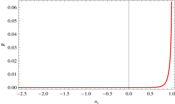
Figure 2: Graph for scalar-tensor ratio verses spectral index for $\lambda=0.5,\sigma=1,A=1,M_{4}=1,f=\frac{3}{7},\psi=\frac{5}{3},\xi_{1}=0.2\times 10^{-8},T=5.47\times 10^{-5};\omega=0.25,\upsilon=1$.

It can be observed from Figure 2 that the scalar-tensor ratio ($r$) remains less than $0.88$ for the range of spectral index $0.85<n_{s}<0.98$. However, an upper bound for tensor-to-scalar ratio as predicted by the BISEP$2$ [28], WMAP$7$ [29, 30], WMAP$9$ [31] and Plank data [32] are $r<0.26,~{}0.36,~{}0.38,\\ ~{}0.11$ respectively. Hence, our results show the compatibility with mentioned observational data.

Moreover, the scalar spectral index $n_{s}$ can be defined as [33]

$$n_{s}-1=\frac{d\ln{P_{r}}}{d\ln{K}}.$$

Here, wave number $K$ is related to the number of e-folds $N$ through relation $d\ln{K}=-d{N}$. With the help of above equations, $n_{s}$ takes the form as

$$n_{s} = 1+\frac{4^{b_{1}}}{(Af)}\bigg{(}\frac{1}{1+b}\bigg{)}^{1-2b_{1}}\exp\bigg{[}-b_{3}b_{5}\phi^{4b_{1}-2}\bigg{]}\phi^{-2(2+b_{1})}\bigg{(}\frac{f-1}{\upsilon(1+\omega)}\bigg{)}^{-b_{1}}b_{1}$$

$$\times \bigg{[}(11(1+b)\exp\bigg{[}b_{3}b_{5}\phi^{2b_{1}}\bigg{]}-4\exp\bigg{[}b_{3}b_{5}\phi^{4b_{1}-2}\bigg{]}(5f-7))\phi^{2}+8$$

$$\times (1+b)\exp\bigg{[}b_{3}b_{5}\phi^{2b_{1}}\bigg{]}\phi^{2b_{1}}b_{3}((1-b_{1})b_{4}+\phi^{2}b_{1}b_{5})\bigg{]},$$

where

$$b_{2} = \frac{\sqrt{3Af}T}{2\pi^{2}}\bigg{(}\frac{4\pi}{3M_{4}^{2}(Af)^{2}\lambda}\bigg{)}^{2}\bigg{(}\frac{Af}{1-f}\bigg{)}\bigg{(}\frac{f-1}{\upsilon(1+\omega)}\bigg{)}^{\frac{7-5f}{2(1+b)}}\bigg{(}\frac{1}{2(1+b)}\bigg{)}^{\frac{7-5f}{1+b}},$$

$$b_{3} = \frac{3(Af)}{4\psi}\bigg{(}\frac{1}{2(1+b)}\bigg{)}^{2b_{1}}\bigg{(}\frac{f-1}{\upsilon(1+\omega)}\bigg{)}^{b_{1}},$$

$$b_{4} = \bigg{(}\frac{f-1}{\upsilon(1+\omega)}\bigg{)}^{b_{1}}\bigg{(}\frac{4b_{1}(\psi-1)}{b_{1}-1}\bigg{)},$$

$$b_{5} = \bigg{(}\frac{M_{4}^{2}Af\lambda}{4\pi}\bigg{)}\bigg{(}\frac{1}{2(1+b)}\bigg{)}^{2b_{1}}\bigg{(}\frac{\xi_{1}}{2b_{1}-1}\bigg{)}.$$

Figure 3 shows that the value of spectral index $n_{s}$ is compatible with the number of e-folds, which are approximately equal to $30$. According to WMAP$7$ [29, 30], WMAP$9$ [31] and Plank $2015$ [32], the value of spectral index lies in ranges $0.967\pm 0.014$, $0.972\pm 0.013$, and $0.968\pm 0.006$.

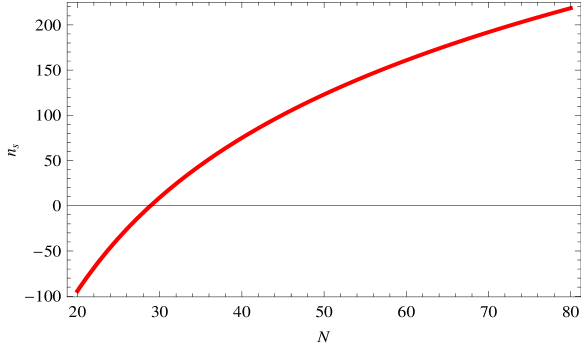
Figure 3: Graph of Spectral index for in term of e-folds for $\lambda=0.5,\sigma=1,A=4,l=1,f=\frac{3}{5},\psi=\frac{4}{3},\xi_{1}=0.2\times 10^{-8},\omega=0.25,\upsilon=1$.

The running of spectral index can be defined as follows [33]

$$\alpha_{s}=\frac{dn_{s}}{d\ln{K}}.$$

By using expression of $n_{s}$, $d\ln{K}=-d{N}$ and Eq.(12), $\alpha_{s}$ leads to

$$\alpha_{s} = \frac{2^{3+4b_{1}}}{(Af)^{2}}\bigg{(}\frac{1}{1+b}\bigg{)}^{1-4b_{1}}\exp\bigg{[}-\phi^{4b_{1}-2}b_{3}b_{5}\bigg{]}\phi^{-4(2+b_{1})}\bigg{(}\frac{-1+f}{\upsilon(1+\omega)}\bigg{)}^{-2b_{1}}b_{1}^{2}$$

$$\times \bigg{[}(-11(1+b)\exp\bigg{[}\phi^{2b_{1}}b_{3}b_{5}\bigg{]}+4\exp\bigg{[}\phi^{-2+4b_{1}}b_{3}b_{5}\bigg{]}(5f-7))\phi^{4}(1+b_{1})$$

$$- 8(1+b)\exp\bigg{[}\phi^{2b_{1}}b_{3}b_{5}\bigg{]}\phi^{6b_{1}}(-1+2b_{1})b_{3}^{2}b_{5}((1-b_{1})b_{4}+\phi^{2}b_{1}b_{5})$$

$$+ (1+b)\exp\bigg{[}\phi^{2b_{1}}b_{3}b_{5}\bigg{]}\phi^{2+2b_{1}}b_{3}(16(b_{1}-1)b_{4}+3\phi^{2}b_{1}b_{5})+(1+b)$$

$$\times \exp\bigg{[}\phi^{2b_{1}}b_{3}b_{5}\bigg{]}\phi^{2+4b_{1}}b_{3}b_{5}\bigg{(}11+2b_{1}(-11+4b_{3}((1-b_{1})b_{4}+\phi^{2}b_{1}b_{5}))\bigg{)}\bigg{]}.$$

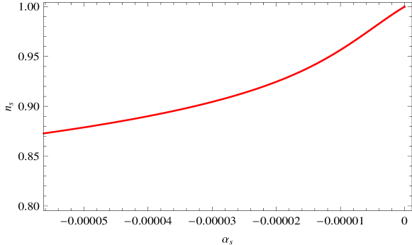
Figure 4: Plot of spectral index with it’s running for $\lambda=0.2,\sigma=1,A=1,M_{4}=1,f=\frac{3}{7},\psi=\frac{4}{3},\xi_{1}=0.2\times 10^{-8},T=5.47\times 10^{-5},\omega=0.25,\upsilon=1$.

Figure 4 represents that spectral index ($n_{s}$) versus running of spectral index is compatible with both observational data. For example, WMAP$7$ observational data has provided the value of spectral index and it’s running which are approximately equal to $1.027\pm 0.051$ and $-0.034\pm 0.026$, respectively. According to WMAP$7$ [29, 30] and WMAP$9$ [31], the value of spectral index and it’s running are approximately equal to $1.009\pm 0.049,0.992\pm 0.019,$ and $-0.019\pm 0.025,-0.019\pm 0.025$ respectively.

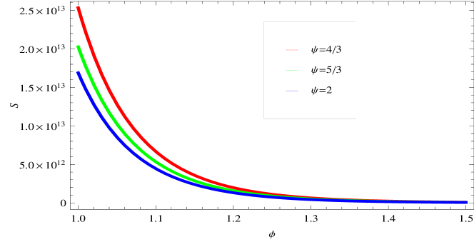
Figure 5: Plot of entropy density $S$ in terms of inflaton $\phi$ use the parametric values as $\lambda=1,\sigma=1,A=1,M_{4}=1,f=\frac{3}{5},\Gamma_{1}=0.275,\xi_{2}=0.2\times 10^{-8},T=5.47\times 10^{-5},\omega=0.25,\beta=0.775,\upsilon=1$.

4.2 Constant Bulk and Dissipative Coefficients

Here, we take $\Gamma=\Gamma_{1}$, $\xi=\xi_{2}$. Under these considerations, $\phi(t)$ and $V(\phi)$ lead to

$$\phi-\phi_{0} = \frac{2}{1+h}\bigg{(}\frac{3\lambda M_{4}^{2}}{4\pi}\bigg{)}^{\frac{1+\sigma}{4}}\bigg{(}\frac{1-f}{\upsilon\Gamma(1+\omega)}\bigg{)}^{\frac{1}{2}}t^{\frac{1+h}{2}},$$

$$V = (Af)^{2}\bigg{(}\frac{1+h}{2}\bigg{)}^{\frac{4(f-1)}{1+h}}\bigg{(}\frac{4\pi}{3\lambda l^{2}}\bigg{)}^{\frac{(1+\sigma)(f-1)}{(1+h)}-1}\bigg{(}\frac{\upsilon\Gamma_{1}(1+\omega)}{1-f}\bigg{)}^{\frac{2(f-1)}{1+h}}\phi^{\frac{4(f-1)}{1+h}},$$

where $h=(f-1)(1+\sigma)$. In this case, entropy density reduces to

$$S = \bigg{(}\frac{Af}{T\psi}\bigg{)}\bigg{(}\frac{1+h}{2}\bigg{)}^{\frac{2(f-1)}{1+h}}\bigg{(}\frac{4\pi}{3\lambda M_{4}^{2}}\bigg{)}^{\frac{(1+\sigma)(f-1)}{2(1+h)}-1}\bigg{(}\frac{\upsilon\Gamma_{1}(1+\omega)}{1-f}\bigg{)}^{\frac{(f-1)}{1+h}}\phi^{\frac{2(f-1)}{1+h}}$$

$$\times \bigg{[}\frac{(Af)^{2}}{\Gamma_{1}}\bigg{(}\frac{4(f-1)}{1+h}\bigg{)}^{2}\bigg{(}\frac{1+h}{2}\bigg{)}^{\frac{4(f-1)}{1+h}}\bigg{(}\frac{4\pi}{3\lambda M_{4}^{2}}\bigg{)}^{\frac{(1+\sigma)(f-1)}{(1+h)}}\phi^{\frac{4(f-1)}{1+h}-2}$$

$$\times \bigg{(}\frac{\upsilon\Gamma_{1}(1+\omega)}{1-f}\bigg{)}^{\frac{2(f-1)}{1+h}}+\xi_{2}\bigg{]}.$$

Its plot versus $\phi$ is shown in Figure 5 which also remains positive as well as exhibits the decreasing behavior for three different values of $\psi$. The slow-roll parameter $\epsilon$ is obtained for this case is

$$\epsilon=\frac{1-f}{Af}\bigg{(}\frac{1+h}{2}\bigg{)}^{\frac{-2f}{1+h}}\bigg{(}\frac{4\pi}{3\lambda M_{4}^{2}}\bigg{)}^{\frac{-(1+\sigma)f}{2(1+h)}}\bigg{(}\frac{\upsilon\Gamma_{1}(1+\omega)}{1-f}\bigg{)}^{\frac{-f}{1+h}}\phi^{\frac{-2f}{1+h}}.$$

For this case, the lower and upper bounds of $\phi$ can be obtained by using $\epsilon\simeq 1$ as

$$\phi_{i} = \bigg{(}\frac{1-f}{Af}\bigg{)}^{\frac{1+h}{2f}}\bigg{(}\frac{2}{1+h}\bigg{)}\bigg{(}\frac{3\lambda M_{4}^{2}}{4\pi}\bigg{)}^{\frac{1+\sigma}{4}}\bigg{(}\frac{1-f}{\upsilon\Gamma_{1}(1+\omega)}\bigg{)}^{\frac{1}{2}},$$

$$\phi_{g} = \bigg{(}\frac{2}{1+h}\bigg{)}\bigg{(}\frac{3\lambda M_{4}^{2}}{4\pi}\bigg{)}^{\frac{1+\sigma}{4}}\bigg{(}\frac{1-f}{\upsilon\Gamma_{1}(1+\omega)}\bigg{)}^{\frac{1}{2}}\bigg{(}\frac{N}{A}+\bigg{(}\frac{1-f}{Af}\bigg{)}\bigg{)}^{\frac{1+h}{2f}}.$$

The auxiliary function turns out to be

$$\chi(\phi) = \frac{3}{2}\bigg{(}\frac{1-f}{1+h}\bigg{)}\ln\phi.$$

The scalar power spectra and corresponding amplitude in this case becomes

$$P_{r} = \frac{(Af)^{\frac{3}{2}}T_{r}}{2\sqrt{\Gamma_{1}}\pi^{2}(1-f)}\bigg{(}\frac{1+h}{2}\bigg{)}^{\frac{5-3f}{1+h}}\bigg{(}\frac{4\pi}{3\lambda M_{4}^{2}}\bigg{)}^{\frac{2(1+\sigma)f-5h+6}{4(1+h)}}\bigg{(}\frac{\upsilon\Gamma_{1}(1+\omega)}{1-f}\bigg{)}^{\frac{5-3f}{2(1+h)}}$$

$$\times \phi^{\frac{-2}{1+h}},$$

$$A_{g}^{2} = \frac{(Af)^{2}}{2\pi^{2}}\bigg{(}\frac{1+h}{2}\bigg{)}^{\frac{4(f-1)}{1+h}}\bigg{(}\frac{4\pi}{3\lambda M_{4}^{2}}\bigg{)}^{\frac{h}{(1+h)}}\bigg{(}\frac{\upsilon\Gamma_{1}(1+\omega)}{1-f}\bigg{)}^{\frac{2(f-1)}{1+h}}\phi^{\frac{4(f-1)}{1+h}}$$

$$\times \coth\bigg{[}\frac{K}{2T}\bigg{]}.$$

The tensor-to-scalar ratio becomes

$$r(K_{0}) = \frac{(Af)^{4}(1-f)}{T_{r}}\sqrt{\frac{\Gamma_{1}}{Af}}\bigg{(}\frac{1+h}{2}\bigg{)}^{\frac{7f-9}{1+h}}\bigg{(}\frac{4\pi}{3\lambda M_{4}^{2}}\bigg{)}^{\frac{9h-6-2f(1+\sigma)}{4(1+h)}}\phi^{\frac{4f-2}{1+h}}$$

$$\times \bigg{(}\frac{\upsilon\Gamma_{1}(1+\omega)}{1-f}\bigg{)}^{\frac{7f-9}{2(1+h)}}\coth\bigg{[}\frac{K}{2T}\bigg{]}.$$

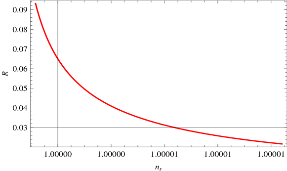
Figure 6: Plot for scalar-tensor ratio verses spectral index for $\lambda=1,\sigma=1,A=5,M_{4}=1,f=\frac{3}{5},\psi=\frac{4}{3},T=5.47\times 10^{-5},\Gamma_{1}=0.75,\omega=0.25,\beta=0.775,P=2.541\times 10^{4},K=0.002$.

The plot of this tensor-to-scalar ratio is shown in Figure 6 and we obtain $r<0.11$ in the present scenario. However, the WMAP$7$, WMAP$9$ and Plank data [29, 30] predict an upper bound for tensor-to-scalar ratio $r<0.36,0.38,0.11$ for spectral index $n_{s}=0.982\pm 0.020,~{}0.992\pm 0.019,~{}0.9655\pm 0.0062$ respectively. The scalar spectral index leads to

$$n_{s} = 1+\frac{\Gamma_{1}}{2(Af)^{2}(1-f)}\bigg{(}\frac{1+h}{2}\bigg{)}^{\frac{6(1-f)}{1+h}}\bigg{(}\frac{4\pi}{3\lambda M_{4}^{2}}\bigg{)}^{1-\frac{3h}{2(1+h)}}\bigg{(}\frac{\upsilon\Gamma_{1}(1+\omega)}{1-f}\bigg{)}^{\frac{3(1-f)}{1+h}}$$

$$\times \phi^{\frac{6(1-f)}{1+h}}.$$

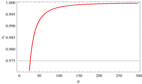
Figure 7: Plot of Spectral index in term of e-folds for $\lambda=0.2,\sigma=1,A=3,M_{4}=1,f=\frac{3}{5},T=5.47\times 10^{-5},\Gamma_{1}=0.275,\omega=0.25,\upsilon=1$.

Figure 7 shows that the value of spectral index $0.96<n_{s}<0.97$ is compatible with the number of e-folds, which are approximately equal to $30$ (WMAP$7$ [29, 30], WMAP$9$ [31] and Plank 2015 [32]). The $\alpha_{s}$ takes the following form

$$\alpha_{s} = \frac{3\Gamma_{1}^{2}}{4(f-1)(Af)^{5}}\bigg{(}\frac{1+h}{2}\bigg{)}^{\frac{12(1-f)}{1+h}}\bigg{(}\frac{4\pi}{3\lambda M_{4}^{2}}\bigg{)}^{-1+\frac{3}{1+h}}\bigg{(}\frac{\upsilon\Gamma_{1}(1+\omega)}{1-f}\bigg{)}^{\frac{6(1-f)}{1+h}}$$

$$\times \phi^{\frac{12(1-f)}{1+h}}.$$

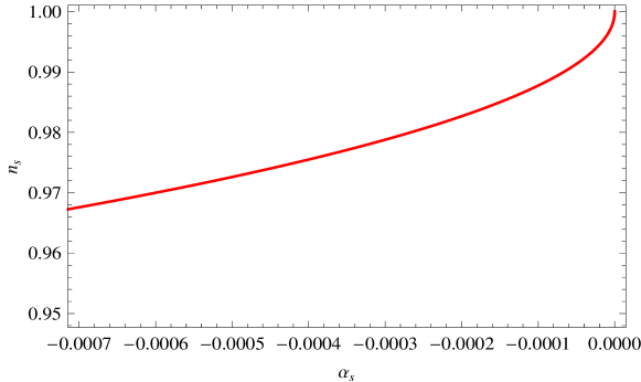
Figure 8: Plot of spectral index with it’s running for $\lambda=0.5,\sigma=1,A=3,M_{4}=1,f=\frac{3}{5},\psi=\frac{4}{3},\xi_{2}=3.2\times 10^{-8},T=5.47\times 10^{-5},\omega=0.25,\Gamma_{1}=0.275,\beta=0.775,\upsilon=1$.

Figure 8 represents that running of spectral index is compatible with both observational data (WMAP $7+9$) for constant bulk and dissipative coefficients.

5 Conclusion

We have considered the warm intermediate MCG inflationary scenario on the brane with bulk viscous pressure and high dissipative regime in flat FRW universe. We have calculated the slow-roll parameters, number of e-folds, scalar-tensor power spectra, spectral indices, tensor scalar ratio and running of scalar spectral index. We have analyzed these parameters for variable as well as constant dissipation and bulk viscous coefficients. We have restricted constant parameters involving in the models according to WMAP$7$ results for examining the physical behavior of $n_{s}-N$, $n_{s}-r$ and $n_{s}-\alpha_{s}$ trajectories in both cases of dissipation and bulk viscous coefficients. We have chosen model parameters of MCG as $\omega=0.25,~{}\sigma=1,~{}\beta=0.775$ which lies within the constraints $(-1.186,0.2754),~{}(-0.9469,1.442)$ and $(0.0497,0.9935)$ obtained by [34], respectively.

The entropy density has been displayed versus scalar field ($\phi$) (Figure 1 and 5) which shows increasing behavior and remains positive (as expected) for both cases of dissipation and bulk viscous coefficients. The standard values of tensor-scalar ratio $r<0.36,~{}0.38,~{}0.11$ for spectral index $n_{s}=0.982\pm 0.020,~{}0.992\pm 0.019,~{}0.9655\pm 0.0062$ according to WMAP$7$ [29, 30], WMAP$9$ [31] and Plank 2015 [32] result respectively. In our case, the tensor-scalar ratio versus spectral index is compatible with this observational data (Figure 2 and 6). We have also observed from Figures (3 and 7) that the trajectories of spectral index lies within the suggested ranges of observations for approximately $30$ number of e-folds, i.e., $n_{s}=1.027\pm 0.051,~{}1.009\pm 0.049,~{}0.096\pm 0.025$ and $\alpha_{s}=-0.034\pm 0.026,~{}-0.019\pm 0.025,~{}-0.0084\pm 0.0082$ according to WMAP$7$ [29, 30], WMAP$9$ [31] and Plank 2015 [32], respectively. We have also attained the compatibility of spectral index and it’s running with the before mentioned observational schemes (Figures 4 and 8).

In [35], we have examined the possible realization of warm chaotic inflation and logamediate inflation within the framework of a MCG brane-world model by assuming the standard scalar field. We have investigated the slow-roll parameters, number of e-folds, scalar-tensor power spectra, spectral indices, tensor scalar ratio and running of scalar spectral index for variable as well as constant dissipation and bulk viscous coefficients. We have found $r<0.11$, $n_{s}=0.96\pm 0.025$ and $\alpha_{s}=-0.019\pm 0.025$ and these ranges are consistent with BICEP$2$, WMAP $(7+9)$ and Planck data [35]. Also, we have investigated the MCG inspired inflationary regime in the brane-world framework in the presence of standard and tachyon scalar fields [36].

We have developed the $n_{s}-N$ and $r-N$ planes and concluded that $n_{s}\simeq 96^{+0.5}_{-0.5}$ and $r\leq 0.0016$ for $N\simeq 60^{+5}_{-5}$ in both cases of scalar field models as well as for all values of $m$ and these constraints are consistent with observational data such as WMAP$7$, WMAP$9$ and Planck data [36]. We have also explored warm inflationary universe models by assuming with various chaplygin gas models with $\Gamma\propto T$, weak and strong dissipative regimes and quartic potential $\frac{\lambda_{*}\phi^{4}}{4}$ [37]. We have observed that the $r<0.05$ in generalized chaplygin gas, $r<0.15$ in modified chaplygin gas, and $r<0.12$ in generalized cosmic chaplygin gas models and these are in agreement with WMAP$9$ and latest Planck data.

The present work is different from [35, 36, 37]. We have explored the role of bulk viscous pressure on the warm intermediate inflationary MCG in brane-world framework by taking standard scalar field. We have found that the behavior of entropy density in the current scenario ensures the validity of thermodynamics laws. We have illustrated the results $n_{s}-N$, $n_{s}-r$ and $n_{s}-\alpha_{s}$ for variable as well as constant dissipation and bulk viscous coefficients at high dissipative regime and found that these parameters are compatible with recent observational data such as WMAP $7+9$, BICEP$2$ and Planck data.

References

• [1] Campo, S. D., Gonzalez, C. and Herrera, R.: Astrophys. Space Sci. 358(2015)31.
• [2] Herrera, R., Videla, N. and Olivares, M.: Eur. Phys. J. C. 75(2015)205.
• [3] Herrera, R., Videla, N. and Olivares, M.: Int. J. Mod. Phys. D 23(2014)1450080.
• [4] Setare, M. R. and Kamali, V.: Phys. Lett. B 739(2014)68 73.
• [5] Berera, A.: Phys. Rev. Lett. 75(1995)3218; ibid: Phys. Rev. D 55 (1997) 3346.
• [6] Mimoso, J.P., Nunes, A. and Pavon, D.: Phys. Rev. D 73(2006)023502.
• [7] del Campo, S., Herrera R. and Pavon, D.: Phys. Rev. D 75(2007)083518.
• [8] Landau, L. and Lifshitz, E.M.: Mecanique des Fluides (MIR, Moscow, 1971); Huang, K.: Statistical Mechanics (J. Wiley, New York, 1987).
• [9] Guth, A.H. and Pi, S.Y.: Phys. Rev. Lett. 49(1982)1110.
• [10] Setare, M.R. and Kamali, V.: Phy. Lett. B 739(2014)68.
• [11] Benaoum, H. B.: ArXiv: hep-th/0205140.
• [12] Shiromizu, T., Maeda,K.-I., and Sasaki, M.: Phys. Rev. D 62(2000)024012.
• [13] Barrow, J. D. and Saich, P.: Phys. Lett. B 249(1990)40611.
• [14] Rendall, A. D.: Class. Quantum Grav. 22(2005)1655.
• [15] Barrow, J. D. and Liddle, A. R.: Phys. Rev. D 47(1993)5219.
• [16] Bamba, K. and Odintsov, S.D.: Eur. Phys. J. C 76(2016)18.
• [17] Setare, M. R. and Kamali, V.: Phys. Lett. B 736(2005)86.
• [18] Campo, S. D. and Herrera, R.: Phys. Lett. B 670(2009)266.
• [19] Setare, M. R. and Kamali, V.: Class. Quantum Grav. 32(2015)235005.
• [20] Kamali, V. and Setare, M. R.: arXiv:1508.05479.
• [21] Antonella Cid, M., del Campo, S. and Herrera, R.: JCAP 0710(2007)005.
• [22] Bento, M. C., Bertolami, O. and Sen, A. A.: Phys. Rev. D 70(2004)083519.
• [23] Bamba, K. et al.: Astrophys. Space Sci.  342(2012) 155.
• [24] Benaoum, H. B.: Int. J. Mod. Phys. D 23(2014)1450082.
• [25] Campo, S. D. and Herrera, R.: Phys. Lett. B 653(2007)122.
• [26] Liddle, A. R. and Lyth, D. H.: Phys. Lett. B 291(1992)391-398.
• [27] Sharif, M. and Saleem, R.: MNRAS 450(2015)3802.
• [28] Ade, P. A. R. et al.: Phys. Rev. Lett. 112(2014)241101.
• [29] Komatsu, E. et al.: Astrophys. J. Suppl. 192(2011)18.
• [30] Larson, D. et al.: Astrophys. J. Suppl. 192(2011)16.
• [31] Hinshaw, G. et al.: Astrophys. J. Suppl. 208(2013)19.
• [32] Ade, P. A. R. (Cardiff U.) et al.: arXiv:1502.01589.
• [33] Czerny, M., Kobayashi, T. and Takahashi, F.: Phys. Lett. B 735(2014)176.
• [34] Paul, B.C. and Thakur, P.: JCAP 11(2013)052.
• [35] Jawad, A., Ilyas, A. and Rani, S.: Astropart. Phys. 81(2016)61.
• [36] Jawad, A., Rani, S. and Mohsaneen, S.: Astrophys Space Sci 361(2016)158.
• [37] Jawad, A., Butt, S. and Rani, S.: Eur. Phys. J. C 76(2016)274.